Statistical coupling constants
from hidden sector entanglement

Abstract

String theory predicts that the couplings of Nature descend from dynamical fields. All known string-motivated particle physics models also come with a wide range of possible extra sectors. It is common to posit that such moduli are frozen to a background value, and that extra sectors can be nearly completely decoupled. Performing a partial trace over all sectors other than the visible sector generically puts the visible sector in a mixed state, with coupling constants drawn from a quantum statistical ensemble. An observable consequence of this entanglement between visible and extra sectors is that the reported values of couplings will appear to have an irreducible variance. Including this variance in fits to experimental data gives an important additional parameter that can be used to distinguish this scenario from the case where couplings are treated as fixed parameters. There is a consequent interplay between energy range and precision of an experiment that allows an extended reach for new physics.

1 Introduction

The coupling constants of Nature are not truly “constant.” This, at least, is what string theory predicts since such parameters descend from background values of moduli fields, the low energy remnants of higher-dimensional quantum gravity in our 4D world. Parameters such as the fine structure constant or the top quark Yukawa coupling are better viewed as dynamical—though perhaps heavy—fields.

Indeed, one feature of all known string constructions is that beyond the visible sector there are many additional degrees of freedom. These include moduli (see [1, 2, 3]), as well as large numbers of hidden sectors (see [4]) which may only weakly interact with the visible sector, typically through the mediation of the moduli fields. These possibilities pose a challenge in constructing phenomenologically viable UV complete models, but also present an opportunity to access string-motivated signatures of physics beyond the Standard Model.

Here, we observe that moduli fields that interact with hidden sectors will necessarily be entangled with them. If so, following the standard rules of quantum mechanics, we should trace out the hidden sector fields, thus deriving an effective description of the moduli as being in a mixed quantum state. In other words, the visible universe will be described by a quantum statistical ensemble over couplings. We explain how to derive this ensemble, and describe scenarios where there will be a measurable effect. In comparing with experiment, this additional irreducible source of variance will generically produce a different fit to the available data. This provides a way to distinguish this scenario from the case where the couplings are treated as fixed parameters.

2 The Visible Sector and Beyond

Observationally, the visible sector is constructed from all the degrees of freedom in the Standard Model, including 4D gravity. Observables of this theory are often couched in terms of the particle content and possible interaction terms, as governed by the coupling constants of a low energy effective field theory. Letting $\mathcal{H}_{\text{vis}}$ denote the Hilbert space of states for the visible sector, there is a whole family of possible ground states $\lvert\{\lambda\}\rangle\in\mathcal{H}_{\text{vis}}$ labelled by the couplings of the theory.

The general message from string theory is that continuous couplings are really background values for dynamical fields. This motivates promoting these couplings to spacetime-dependent parameters $\{\lambda(x)\}$, and correspondingly time dependent states $\lvert\{\lambda(\vec{x},t)\}\rangle\in\mathcal{H}_{\text{vis}}$. In fact, to capture the full effects of this and other possible string-motivated degrees of freedom, it is more appropriate to enlarge the associated Hilbert space. In what follows, we shall assume that there is an approximate factorization of the full Hilbert space as:

$$\mathcal{H}_{\text{full}}\approx\mathcal{H}_{\text{vis}}\otimes\mathcal{H}_{\overline{\text{vis}}}\,,$$ (1)

where the factor $\mathcal{H}_{\overline{\text{vis}}}$ denotes everything “other than the visible sector.”

This sort of factorization is well-motivated in the context of string constructions (see, e.g., [5] for an early review of some F-theory examples) since the Standard Model is typically localized on a subspace of the full higher-dimensional system, and many extra sectors are sequestered at other locations of the extra-dimensional geometry. There can still be mixing between these sectors through bulk modes such as closed string moduli, which permeate the extra-dimensional geometry, and there are Swampland arguments that some such mixing is irreducible [6]. In such cases, additional structure is present, and we can write:

$$\mathcal{H}_{\overline{\text{vis}}}=\mathcal{H}_{\text{bulk}}\otimes\mathcal{H}_{\text{extra}}^{(1)}\otimes\dots\otimes\mathcal{H}_{\text{extra}}^{(N)}\,,$$ (2)

in the obvious notation (see Fig. 1).

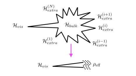
Figure 1: Depiction of the many QFT sectors of a string compactification. Performing a partial trace over the complement of the visible sector yields an effective density matrix for the visible sector couplings.

There are clearly a wide range of possibilities for the dynamics in $\mathcal{H}_{\overline{\text{vis}}}$. If all the mass scales of non-visible sector states are heavy, it is appropriate to use the general framework of effective field theory, integrating out the heavy modes. In the visible sector, this will be encoded in a particular structure for a low energy effective action for visible sector states.

It can also happen, however, that the states of the extra sector are light, perhaps comparable with their visible sector counterparts. In such cases, integrating out these degrees of freedom would result in a non-local effective action in the visible sector. One (practically quite cumbersome) way to track the effects of such extra sectors is via non-analytic behavior in various correlation functions/scattering amplitudes.

We will purse an alternative approach, by treating the visible sector as an open system. Letting $\rho_{\text{full}}$ denote the density matrix for the full system, we obtain a reduced density matrix $\rho_{\text{vis}}\in\mathcal{H}_{\text{vis}}\otimes\mathcal{H}_{\text{vis}}^{*}$ for just the visible sector by performing a partial trace over the complement:

$$\rho_{\text{vis}}=\operatorname{Tr}_{\mathcal{H}_{\overline{\text{vis}}}}\rho_{\text{full}}\,.$$ (3)

So even if $\rho_{\text{full}}$ is a pure state, such as the ground state of the full system, the reduced density matrix will typically be a mixed state. We will focus on the part of this mixed state that involves the couplings. Note also that since there could be some unknown dynamics in the extra sector, we should treat $\rho_{\text{vis}}(t)$ as a time-dependent state. From the perspective of string compactification, this really is a geometric entanglement, since it involves tracing over all regions of the geometry other than where the visible sector is localized. Some explicit examples of stringy brane systems where this sort of entanglement across different sectors was considered include references [7, 8].

On general grounds, the mixed state $\rho_{\text{vis}}$ will involve a sum over possible spacetime configurations for the couplings $\{\lambda(\vec{x},t)\}$, which we summarize schematically as:

$$\rho_{\text{vis}}=\sum_{\lambda,\lambda^{\prime}}\rho_{\text{vis}}(\lambda,\lambda^{\prime})\lvert\lambda\rangle\langle\lambda^{\prime}\rvert\,.$$ (4)

Said differently, the partial trace over the complement of the visible sector produces a quantum statistical ensemble over spacetime-dependent couplings.

3 Example: Coupled Oscillators

The general considerations are already clear in the simple example of a pair of coupled oscillators with a Hamiltonian

$$H=\frac{1}{2}\mathopen{}\mathclose{{}\left(p_{x_{1}}^{2}+p_{x_{2}}^{2}}\right)+\frac{1}{2}\mathopen{}\mathclose{{}\left(\omega_{1}^{2}x_{1}^{2}+\omega_{2}^{2}x_{2}^{2}+\lambda x_{1}x_{2}}\right)\,.$$ (5)

We will think of $x_{1}$ as a modulus field and $x_{2}$ as a field in the hidden sector. There may be additional interactions between $x_{1}$ and other visible sector degrees of freedom, but we neglect them here because we are interested in the effect on $x_{1}$ of tracing over $x_{2}$. The general case of coupling to many hidden sector oscillators is treated in Appendix A.

We can diagonalize this Hamiltonian in terms of the variables $y_{1}=x_{1}\cos\alpha-x_{2}\sin\alpha$ and $y_{2}=x_{1}\sin\alpha+x_{2}\cos\alpha$ with the mixing angle specified by $\tan 2\alpha=\lambda/(\omega_{2}^{2}-\omega_{1}^{2})$. The Hamiltonian becomes

$$H=\frac{1}{2}\mathopen{}\mathclose{{}\left(p_{y_{1}}^{2}+p_{y_{2}}^{2}}\right)+\frac{1}{2}\mathopen{}\mathclose{{}\left(\omega_{1}^{\prime 2}y_{1}^{2}+\omega_{2}^{\prime 2}y_{2}^{2}}\right)\,,$$ (6)

where $\omega_{1}^{\prime 2}=\omega_{1}^{2}-(\lambda/2)\tan\alpha$ and $\omega_{2}^{\prime 2}=\omega_{2}^{2}+(\lambda/2)\tan\alpha$. The ground state is then a product of Gaussians in $y_{1}$ and $y_{2}$.

Converting back to the original physical variables we find the ground state wavefunction

$$\psi_{0}=\frac{(\det A)^{1/4}}{\sqrt{\pi}}e^{-\frac{1}{4}\mathopen{}\mathclose{{}\left(\frac{x_{1}^{2}}{\tau_{1}^{2}}+\frac{x_{2}^{2}}{\tau_{2}^{2}}+\frac{2x_{1}x_{2}}{g}}\right)}\,,\quad A=\begin{pmatrix}\frac{1}{2\tau_{1}^{2}}&1/2g\\ 1/2g&\frac{1}{2\tau_{2}^{2}}\end{pmatrix}$$ (7)

where

$$\frac{1}{2\tau_{1}^{2}}=\omega_{1}^{\prime}\cos^{2}\alpha+\omega_{2}^{\prime}\sin^{2}\alpha\,,\quad\frac{1}{2\tau_{2}^{2}}=\omega_{2}^{\prime}\cos^{2}\alpha+\omega_{1}^{\prime}\sin^{2}\alpha\,,\quad\frac{1}{2g}=\mathopen{}\mathclose{{}\left(\omega_{2}^{\prime}-\omega_{1}^{\prime}}\right)\sin\alpha\,\cos\alpha\,.$$ (8)

We see that when $g$ is finite, the modulus field $x_{1}$ and the hidden sector field $x_{2}$ are entangled, i.e., their wavefunction does not factorize, and in the $g\to\infty$ limit, the entanglement is weak. Tracing out $x_{2}$ gives a density matrix on $x_{1}$: $\rho=\int\mathop{}\!\mathrm{d}x_{2}\;\psi_{0}(x_{1},x_{2})\,\psi_{0}^{*}(x_{1}^{\prime},x_{2}^{\prime})=\operatorname{Tr}_{x_{2}}(\psi_{0}^{*}\psi_{0})$. We find that

$$\rho(x_{1},x_{1}^{\prime})=\frac{\sqrt{\det A}}{\pi}\sqrt{2\pi\tau_{2}^{2}}e^{-(x_{1}^{2}+x_{1}^{\prime 2})/4\tau_{1}^{2}}e^{\tau_{2}^{2}(x_{1}+x_{1}^{\prime})^{2}/8g^{2}}\,,$$ (9)

from which we can work out the variance of the modulus $x_{1}$ when $x_{2}$ is not observed:

$$\operatorname{Var}(x_{1})=\tau_{1}^{2}\mathopen{}\mathclose{{}\left(1-\frac{\tau_{1}^{2}\tau_{2}^{2}}{g^{2}}}\right)^{-1}\xrightarrow{g\to\infty}\tau_{1}^{2}\mathopen{}\mathclose{{}\left(1+\frac{\tau_{1}^{2}\tau_{2}^{2}}{g^{2}}}\right)\,,$$ (10)

where the equation on the right is in the limit of weak entanglement.

Several qualitative features are clear from these results. Suppose $\lambda=0$, so that the modulus does not interact with the hidden sector. Then the mixing angle is $\alpha=0$, $\omega_{1}^{\prime}=\omega_{1}$, $g=\infty$, $\tau_{1}^{2}=1/2\omega_{1}$, and the variance of $x_{1}$ is simply fixed by the steepness of its potential, $\operatorname{Var}(x_{1})\propto 1/\omega_{1}$, so that a shallow potential (small $\omega_{1}^{2}$) leads to large fluctuations. We want to show that even if the potential for the modulus is steep (large $\omega_{1}^{2}$), the variance of $x_{1}$ can still be large because of the interaction with the hidden sector. Notice that if we tune $\omega_{1}$, $\omega_{2}$, and $\lambda$ so that $g\to\tau_{1}\tau_{2}$ at fixed $\tau_{1}$ and $\tau_{2}$, the variance of $x_{1}$ necessarily becomes large. Mechanistically, this is because even if both $x_{1}$ and $x_{2}$ are stiff directions, their mixing can generate a shallow direction in the combined potential. Large quantum fluctuations along this valley contribute to the variance of $x_{1}$. Here, we are treating the same phenomenon in the language of open quantum systems, with $x_{1}$ entangled with a hidden bath. If there are $N$ independent hidden sector oscillators mixing with with the modulus in this way, even weak mixing can generate a large effect, because the variance will be enhanced as a function of $N$.

4 Entangled Moduli in Field Theory

Let us now turn to the case of a quantum field theory engineered via string theory. A common situation is that we get a Lagrangian which depends on some coupling constants. In the visible sector Lagrangian, this appears through a term of the form:

$$\mathcal{L}_{\text{v}}\supset\lambda_{\text{v}}\mathcal{O}_{\text{v}}\,,$$ (11)

where $\lambda_{\text{v}}$ is a visible sector coupling, and $\mathcal{O}_{\text{v}}$ is a visible sector operator. We promote $\lambda_{\text{v}}$ to a dynamical field $\phi$ with a “decay constant” $f_{\text{v}}$, performing the substitution:

$$\lambda_{\text{v}}\mapsto\lambda_{\text{v}}+\frac{\phi}{f_{\text{v}}}\,.$$ (12)

Doing so motivates us to consider an enlarged Hilbert space that includes the modulus as well as its possible couplings to other sectors. For example, this modulus can appear equally well as a coupling in an extra sector, so we generically expect mixing terms involving visible and hidden sector operators $\mathcal{O}_{\text{v}}$ and $\mathcal{O}_{\text{h}}$:

$$\mathcal{L}_{\text{mix}}=\mathopen{}\mathclose{{}\left(\lambda_{\text{v}}+\frac{\phi}{f_{\text{v}}}}\right)\mathcal{O}_{\text{v}}+\mathopen{}\mathclose{{}\left(\lambda_{\text{h}}+\frac{\phi}{f_{\text{h}}}}\right)\mathcal{O}_{\text{h}}\,.$$ (13)

There is no shortage of examples coming from string theory. For example, if we interpret $\phi$ as a closed string modulus, the associated decay constant might be Planck or GUT scale, some axion models have lower decay constant scales, while in some models where $\phi$ is instead an open string modulus, the scale could be far closer to the TeV range [9], if the mass scales are correlated with supersymmetry breaking.

In most cases, one typically assumes there is some potential that stabilizes the value of $\phi$ at zero. This potential, as well as the various mass scales, decay constants, and number of extra sectors introduces a large number of possibilities, and with it a seemingly endless variety of possible signatures.

We seek a more model independent way to characterize the range of possible signatures. To this end, we can perform a partial trace on $\rho_{\text{full}}$ over the complement of $\mathcal{H}_{\text{vis}}$ states, and thus obtain a mixed state for the visible sector density matrix, with a distribution of possible coupling constants.

Let us now illustrate how the density matrix for couplings comes about. The ground state is constructed by the Euclidean path integral as

$$\langle\Phi,\Phi_{h}|\Psi\rangle=\int^{\Phi,\Phi_{\text{h}},t=0}_{t=-\infty}\mathcal{D}\phi\,\mathcal{D}\phi_{\text{h}}\;e^{-S}\,,$$ (14)

where we have suppressed indices on the visible and hidden sector fields and indicated schematically that the integral sums over all configurations from $t=-\infty$ to $t=0$ with the boundary condition that $\phi(0^{-})=\Phi$ and $\phi_{\text{h}}(0^{-})=\Phi_{\text{h}}$, with capital variables serving to emphasize that these are the spatial profiles of some field at a fixed time. The density matrix for the system

$$\rho=\lvert\Psi\rangle\langle\Psi\rvert\,,$$ (15)

is constructed by multiplying the state vector in Eq. 14 by its conjugate, computed by path integrating from $t=0^{+}$ to $t=\infty$ with the boundary condition $\phi(0^{+})=\Phi^{\prime}$ and $\phi_{\text{h}}(0^{+})=\Phi_{\text{h}}^{\prime}$.

The reduced density matrix for the modulus field is obtained by tracing out the hidden fields:

$$\rho_{\text{red}}=\operatorname{Tr}_{\phi_{\text{h}}}(\lvert\Psi\rangle\langle\Psi\rvert)\,.$$ (16)

In path integral language, this amounts to setting $\phi_{\text{h}}(0^{-})=\phi_{\text{h}}(0^{+})=\Phi_{\text{h}}$ in the integral for the density matrix and then integrating over $\phi_{\text{h}}$ for all times, including the $t=0$ boundary value $\Phi_{h}$. As discussed in [10], this is equivalent to first integrating out the hidden field $\phi_{\text{h}}$ completely to get a quantum effective action $S_{\text{eff}}(\phi)$ for the modulus field, and then doing the construction of the density matrix for $\phi$ with the exponential of the effective action weighting the path sum. From this point of view, the equal time correlation function of operators $\mathcal{O}$ constructed out of the modulus at $t=0$ is

$$\langle\mathcal{O}\mathcal{O}\rangle=\operatorname{Tr}(\mathcal{O}\mathcal{O}\rho_{\text{red}})=\int\mathcal{D}\phi\,\mathcal{D}\phi_{\text{h}}\;\mathcal{O}\,\mathcal{O}\,e^{-S}\,.$$ (17)

To arrive at the expression on the right hand side, we carry out the path integral for the wavefunctional ($\Psi(\Phi,\Phi_{h})=\langle\Phi,\Phi_{h}|\Psi\rangle$) and its conjugate ($\Psi^{*}(\Phi^{\prime},\Phi_{h}^{\prime})=\langle\Psi|\Phi^{\prime},\Phi_{h}^{\prime}\rangle$) to find the density matrix as described above, then sew the boundary conditions across the $t=0$ for the hidden sector ($\Phi_{h}=\Phi_{h}^{\prime}$) and integrate to find the reduced density matrix, and then finally multiply by $\mathcal{O}\mathcal{O}$, sew the boundary conditions for the modulus field $\phi$ across $t=0$ ($\Phi=\Phi^{\prime}$) and integrate to take the trace. Overall, this gives a path integral over the values of the fields at all times as shown. The last expression shows the relation between the reduced density matrix formulation of correlators of $\phi$ and the standard path integral for the same quantities.

We want to work out the density matrix for the modulus $\phi$ in the vacuum state $\lvert 0\rangle$ of our field theory:

$$\rho_{\text{red}}(\Phi,\Phi^{\prime})=\int\mathcal{D}\Phi_{\text{h}}\,\langle\Phi^{\prime},\Phi_{\text{h}}|\Psi\rangle\langle\Psi|\Phi,\Phi_{\text{h}}\rangle=\mathcal{N}\int\mathcal{D}\Phi_{\text{h}}\;\Psi^{*}(\Phi^{\prime},\Phi_{h})\Psi(\Phi,\Phi_{h})\,.$$ (18)

Here $\lvert\Phi,\Phi_{h}\rangle$ is a projector onto the $\Phi$, $\Phi_{h}$ field configuration. We will consider a simple toy model that illustrates the general point, with a quadratic Lagrangian written schematically as

$$\mathcal{L}\sim\phi G\phi+\phi_{\text{h}}^{i}G_{ij}\phi_{\text{h}}^{j}+\phi\lambda_{j}\phi_{\text{h}}^{j}\,.$$ (19)

where we have integrated the action by parts and dropped boundary terms to write the local Lagrangian density in terms of quadratic differential operators $G$ and $G_{ij}$ (e.g., $G\sim\Box+m^{2}$) and the coupling $\lambda_{j}$. The ground state wavefunctional is then

$$\Psi(\Phi,\Phi_{\text{h}}^{i})=\int^{\Phi,\Phi_{\text{h}}^{i},t=0}_{t=-\infty}\mathcal{D}\phi\,\mathcal{D}\phi_{\text{h}}^{i}\;e^{-\int d^{D}x\,\mathcal{L}}\,.$$ (20)

Since the action is quadratic, similarly to the harmonic oscillator example that we described above, the ground state wavefunctional will also be quadratic

$$\Psi(\Phi,\Phi_{\text{h}}^{i})=\sqrt{\mathcal{N}}e^{-\frac{1}{2}\int\mathop{}\!\mathrm{d}^{D-1}x\;\Phi\Omega\Phi+\Phi_{\text{h}}^{i}\Omega_{ij}\Phi_{\text{h}}^{j}+\Phi\epsilon_{j}\Phi_{\text{h}}^{j}}\,,$$ (21)

where $\mathcal{N}$ normalizes $\Psi$. We are being schematic here—strictly speaking, the exponent in the wavefunctional will be a bi-local integral, and $\Omega$, $\Omega_{ij}$ and $\epsilon_{j}$ will be complicated functions of $G$, $G_{ij}$, and $\lambda_{j}$. We will simply be interested in the scaling of these quantities as we intend this as a toy model.

The reduced density matrix is then:

$$\rho_{\text{red}}=\mathcal{N}\int\mathcal{D}\Phi_{\text{h}}^{i}\;\Psi^{*}(\Phi^{\prime},\Phi_{h})\Psi(\Phi,\Phi_{h})\,.$$ (22)

This is a Gaussian integral, and can be evaluated explicitly to give

$$\rho_{\text{red}}=\mathcal{N}e^{-\frac{1}{2}\int\mathop{}\!\mathrm{d}^{D-1}x\;[(\Phi-\Phi^{\prime})(\Omega/2)(\Phi-\Phi^{\prime})+(\Phi+\Phi^{\prime})\Omega_{\text{eff}}(\Phi+\Phi^{\prime})]}\,,$$ (23)

where

$$\Omega_{\text{eff}}=\frac{\Omega}{2}-\frac{1}{8}\epsilon_{i}\Omega_{ij}^{-1}\epsilon_{j}\,.$$ (24)

Finally, we are in a position to evaluate the variance of the modulus field

$$\langle\Phi\Phi\rangle=\operatorname{Tr}(\rho_{\text{red}}\Phi\Phi)=\mathcal{N}\int\mathcal{D}\Phi\;\Phi\,\Phi\,e^{-\int\mathop{}\!\mathrm{d}^{D-1}x\;\Phi\Omega_{\text{eff}}\Phi}\,,$$ (25)

where we set $\Phi=\Phi^{\prime}$ in Eq. 23 and then integrated over $\phi$ to take the trace. Thus, the equal-time variance is

$$\operatorname{Var}(\Phi)=\Omega_{\text{eff}}^{-1}\,.$$ (26)

Again, we are being schematic. More generally we are here really describing the equal time correlation function at some separation, and when the separation is small this correlator measures the variance in the field.

We want to know whether the variance 26 can be large. The basic scale for the variance of $\phi$ is set by the $\Omega$ in the wavefunctional 21. To estimate the effect of the coupling to the hidden sector, let us assume that all the quantities in the wavefunctional have similar orders of magnitude $O(\Omega)\sim O(\Omega_{ij})\sim O(\epsilon_{j})\,\forall i,j$. In fact, for concreteness let us take $\Omega_{ij}\sim\Omega I_{N\times N}$ and $\epsilon_{i}\sim\epsilon\Omega$. Then

$$\Omega_{\text{eff}}\sim\frac{1}{8}(4-\epsilon^{2}N)\Omega\,.$$ (27)

We see that for any $\epsilon$ and $\Omega$, if the number of hidden sector fields $N$ is large, it can easily happen that $\Omega_{\text{eff}}\ll\Omega$, so that $\operatorname{Var}(\phi)\gg 1/\Omega$. (Note that we must have $\epsilon^{2}N<4$ to maintain positive-definiteness of the coupling matrix.) In other words, if there are many hidden sector fields, as there typically are in string theory, they can have a substantial effect on the variance of a heavy modulus field with which they are weakly coupled. Alternatively, we can imagine that the hidden sector fields are lighter than the modulus, as there is nothing forbidding this. This means that $\lvert\Omega_{ij}\rvert\ll\lvert\Omega\rvert$, and can also lead to a small $\Omega_{\text{eff}}$ and thus a large variance for the modulus field.

As we will discuss below, in typical experiments the interactions occur at different times, so we are really interested in the unequal time correlators of $\phi$. To study this in the language of the reduced density matrix, we must time-evolve it, a dynamics that is typically not Hamiltonian, but controlled rather by the Lindblad equation, unless the measurements are appropriately coarse-grained in time [11].

5 Couplings and Correlators

In the previous sections we emphasized that tracing over the extra sector states means that in general, the visible sector actually probed by experiment is really in a mixed state, and consequently, that there is a statistical ensemble of possible values for the coupling constants. Note that even at equal times this can lead to non-trivial spatial correlations for couplings. In practice, carrying out explicit calculations in this setup is somewhat awkward because the very appearance of a wavefunction references a preferred time slicing of our spacetime. If our eventual aim is to extract observables as obtained from a scattering experiment, we should also seek out a treatment which is suitably Lorentz covariant. Again taking our cue from string theory where such couplings descend from moduli fields, we know that the appropriate way to analyze such structures is in terms of the Lorentz covariant correlation functions of the moduli fields. We can visualize this as breaking up the spacetime into small four-dimensional “pixels” and assigning a particular value of the coupling in each such pixel. In the limit where the pixels are quite small, we expect the correlation function to assume a delta function approximation:

$$\langle\lambda(x)\lambda(x^{\prime})\rangle\sim cM_{\text{UV}}^{-4}\delta^{4}(x-x^{\prime}),$$ (28)

with $M_{\text{UV}}$ some UV mass scale, and $c$ a model dependent parameter.

Suppose now that we perform a scattering experiment involving visible sector states. The amplitude can be packaged as a correlation function of visible sector operators $\mathcal{O}_{\text{vis}}^{(i)}$ evaluated in the mixed state $\rho_{\text{vis}}(t)$ obtained by tracing over both bulk moduli and extra sector states:

$$i\mathcal{M}\sim\operatorname{Tr}_{\mathcal{H}_{\text{vis}}}\mathopen{}\mathclose{{}\left(\rho_{\text{vis}}(t)\mathcal{O}_{\text{vis}}^{(1)}\dotsm\mathcal{O}_{\text{vis}}^{(n)}}\right)\,.$$ (29)

One can first perform all visible sector correlation functions, and then perform a further evaluation of all correlators involving the couplings. This is valid to do in a decoupling limit of string theory, and is reminiscent of the procedure one adopts in disorder averaging, though the interpretation is somewhat different.

When we report the value of a coupling constant, we are working backwards from the measured cross section to a corresponding scattering amplitude to extract the value of the coupling constants in our underlying theory. Let us call this reported value of the coupling $\lambda_{\text{expt}}$. This of course comes with a central value as well as some variance. As one improves the precision of an experiment, one expects to reduce this variance.

But, as we have already seen, by treating the visible sector as an open system, there is always an irreducible amount of variance we get just from tracing over everything other than the visible sector. In fact, we can estimate the impact of this just by comparing the values of scattering amplitudes we get by treating $\lambda(\vec{x},t)$ as a statistical parameter. For example, if we have a specific model of physics beyond the visible sector in mind, we can extract the two-point function for couplings via

$$\operatorname{Tr}_{\mathcal{H}_{\text{vis}}}(\rho_{\text{vis}}(t)\lambda(x)\lambda(x^{\prime}))=\operatorname{Tr}_{\mathcal{H}_{\text{full}}}(\rho_{\text{full}}\lambda(x)\lambda(x^{\prime}))\,,$$ (30)

that is, by evaluating the two-point function in the full Hilbert space.

Such perfect knowledge of the extra sectors is typically unavailable. This motivates seeking alternative ways to package the possible effect on visible sector observables. Along these lines, we can think of an observer performing an experiment at some energy scale $Q_{\text{expt}}$ as “sampling” from a probability distribution of couplings. Each point in space and time gives a unique sampled value.

Our observer works in a small spacetime volume of size $\mathop{\rm Vol}\nolimits_{\text{4D}}\sim Q_{\text{expt}}^{-4}$. In each such chunk, they can approximate the sampled value of the coupling by a pure number, call it $\lambda_{\text{expt}}$. We assume the leading order variation of the probability distribution is governed by a Gaussian centered on $\lambda_{\text{expt}}=\lambda_{0}$ (as happens in the ground state of the harmonic oscillator):

$$P(\lambda_{\text{expt}})\sim\exp\mathopen{}\mathclose{{}\left(-\frac{(\lambda_{\text{expt}}-\lambda_{0})^{2}}{2(\Delta\lambda_{\text{expt}}^{2})}+\dotsb}\right)\,,$$ (31)

with variance:

$$\Delta\lambda_{\text{expt}}^{2}\sim\mathopen{}\mathclose{{}\left(\mathop{\rm Vol}\nolimits_{\text{4D}}\times M_{*}^{4}}\right)^{-1}=Q_{\text{expt}}^{4}/M_{*}^{4}\,.$$ (32)

Here, $M_{*}$ is some characteristic mass scale that folds in all the information of the extra sectors. In actual scenarios, the specific details for how this scale is generated could be wildly different. None of this matters for this class of observables. The volume dependence can be tracked by considering the integrals involved in computing a correlator. But, conceptually, we can think about it by imagining that in an experimental volume $\mathop{\rm Vol}\nolimits_{\text{4D}}\sim Q_{\text{expt}}^{-4}$, every appearance of a coupling in a process is averaged via the path sum over independent samples at a number of points that is proportional to this volume. Then we can estimate that the standard deviation of the apparent coupling will decrease by a factor $1/\sqrt{\mathop{\rm Vol}\nolimits_{\text{4D}}}$ and thus the variance will be suppressed by $1/\mathop{\rm Vol}\nolimits_{\text{4D}}$.

Standard lore holds that since we are at energies low compared to the scale at which the modulus fluctuates, we can treat the couplings as frozen, position-independent parameters. Indeed, if $Q_{\text{expt}}$ is far below $M_{*}$, we have a sharply peaked Gaussian. This, however, only covers a subset of well-motivated possibilities, even when the modulus is heavy. Indeed, as seen in the example of a harmonic oscillator in Appendix A, the “extra sector” could consist of many additional light degrees of freedom. The general point is that if there are many extra sectors, and especially if some are at strong coupling, there is a general broadening of the associated distribution of couplings.

6 Signatures

We now ask whether it is possible to measure this effect in actual experiments. A common way to look for extra sectors is to study apparent violations of conservation laws, e.g., missing transverse energy signals. This only covers some models. Examples include effects from soft radiation to an extra sector. The point of the present approach is that even in the absence of more direct signatures, it is still possible to look for potential effects from such sectors.

A nonzero measured variance in the couplings will show up in processes that scale with different powers of the couplings, and consequently the difference $\Delta\lambda_{\text{expt}}^{2}=\langle\lambda_{\text{expt}}^{2}\rangle-\langle\lambda_{\text{expt}}\rangle^{2}$. Note that an effect suppressed by more insertions of the coupling can easily be overcome by kinematic effects, namely a bigger jump in the transition energies of the system. We leave an exhaustive study of possible signatures for future work.

Our relation between effective mass scales and the distance scale being probed extends the traditional “reach” of an experiment. If we observe a null result at some energy scale $Q_{\text{expt}}$ and precision $\Delta\lambda_{\text{expt}}$, then we get a mass scale limit:

$$M_{\text{limit}}=\lvert\Delta\lambda_{\text{expt}}\rvert^{-1/2}Q_{\text{expt}}\,.$$ (33)

The best limits can be set either by having a very precise measurement, or alternatively, going to much higher energy scales. We take as representative examples atomic physics experiments and collider physics experiments:

$$Q_{\text{atomic}}\sim$10\text{\,}\mathrm{eV}$\,,\quad Q_{\text{collider}}\sim$1\text{\,}\mathrm{TeV}$\,.$$ (34)

The current precision of the fine structure constant is on the order of $\sim 10^{-10}$, and one can anticipate determining some couplings at the LHC at the level of $\sim 10^{-2}$, as in [15]. Plugging in for these quantities, we see that depending on the coupling constant and the underlying mass scales, we can set limits:

$$M^{\text{atomic}}_{\text{limit}} \sim$1\text{\,}\mathrm{MeV}$\times\mathopen{}\mathclose{{}\left(\frac{\Delta\lambda_{\text{expt}}}{10^{-10}}}\right)^{-1/2}\times\mathopen{}\mathclose{{}\left(\frac{Q_{\text{atomic}}}{$10\text{\,}\mathrm{eV}$}}\right)\,,$$

$$M^{\text{collider}}_{\text{limit}} \sim$10\text{\,}\mathrm{TeV}$\times\mathopen{}\mathclose{{}\left(\frac{\Delta\lambda_{\text{expt}}}{10^{-2}}}\right)^{-1/2}\times\mathopen{}\mathclose{{}\left(\frac{Q_{\text{collider}}}{$1\text{\,}\mathrm{TeV}$}}\right)\,,$$

so in both cases, the effective reach of an experiment is extended. Perhaps surprisingly, the loss in precision in collider experiments is compensated for by the increase in energy. This is because the variance of our random variable depends on the resolution length of our experiment.

Because measurements have quantum contributions to their variances, a direct measurement of this effect may appear challenging. For example, measuring the variance in the fine-structure constant by observing the line width of a fine-structure transition would be difficult because of the intrinsic line width of the transition. Instead, because measurements are in general sensitive to the square of a matrix element and hence $\langle\lambda_{\text{expt}}^{2}\rangle=\langle\lambda_{\text{expt}}\rangle^{2}+\Delta\lambda_{\text{expt}}^{2}$, the apparent coupling strength will vary with $\Delta\lambda_{\text{expt}}^{2}=(Q_{\text{expt}}/M_{\ast})^{4}$. This leads to an additional source of energy dependence in the observed values of couplings.

7 Discussion and Future Directions

A very general feature of string constructions is the appearance of many extra sectors beyond the visible sector. In this work we have explored one of the consequences of this visible/extra sector entanglement through the resulting statistical distribution of couplings.

The main idea pursued in this work is that a helpful way to organize our thinking about the impact of such extra sectors on the visible sector is in the framework of quantum entanglement. This alone makes it clear that the visible sector is in general not in the ground state, but rather, is in a mixed state. In general this can lead to a wide variety of possible effects but a model independent and rather generic feature of this sort of construction is that there is a statistical distribution of couplings. From a practical standpoint, this suggests that in fitting data to theory one should at least allow this additional variance as an additional measurable feature.

Having seen that we are really dealing with a mixed state in the visible sector, one might naturally ask whether there are other observational consequences. In fact, there is a sense in which one implicitly does this whenever one discusses the “dressed in and out states” appearing in a scattering amplitude, since there are can be various soft processes that are absorbed into these definitions. It would be interesting to use the present work as a general way to parameterize one’s ignorance about asymptotic scattering states.

Our analysis is reminiscent of an old proposal by Coleman [16], which argued that an ensemble of wormholes would also lead to a statistical distribution of physical parameters (for a recent assessment, see, e.g., [17]). The statistical nature of couplings considered here is specified over points in spacetime, whereas in Coleman’s case only a single homogeneous value appears. Phenomenologically, there is no issue with this; it simply reflects the fact that our couplings really descend from dynamical degrees of freedom. Our result hinges on entanglement between a visible sector and an extra sector. According to [18], such entanglement can perhaps be interpreted as a wormhole joining geometrically separated regions of a string compactification. In this sense, the present analysis provides a precise framework for implementing Coleman’s original proposal! Along these lines, it is natural to ask about the impact of tracing over all sectors (including the Standard Model) other than those associated with 4D gravity. At low energies, this leads to a statistical distribution for Newton’s constant and the cosmological constant. Several recent toy models of quantum gravity feature the appearance of a distribution over couplings [19, 20, 21, 22, 23] over which the theory averages. Perhaps these distributions are appearing because all of these theories should really be understood as reduced versions of a complete theory with many unobserved degrees of freedom.

More generally, we can also contemplate the observational consequences of treating the visible sector as an open system. This would also suggest potential signatures such as an apparent loss of unitarity and/or CPT violation. For example, precision fits on the unitarity triangle of the CKM matrix are on the order of $0.001\%$ to $0.05\%$, and remain quite poorly constrained for the PMNS matrix [24]. Cosmological variation in the value of the couplings provides another novel signature [25].

All of this points to an exciting new program for probing the stringy origin of couplings which cuts across several different frontiers of fundamental physics.

Acknowledgments

We thank F. Apruzzi, N. Arkani-Hamed, C. Csáki, M. DeCross, A. Kar, C. Mauger, B. Ovrut, O. Parrikar, R. Penco, C. Rabideau, M. Reece, J. Ruderman, J. Sakstein, A. Solomon and E. Thomson for helpful discussions. The work of VB is supported by the Simons Foundation #385592 through the It From Qubit Simons Collaboration, by the DOE through DE-SC0013528, and the QuantISED program grant DE-SC0020360. The work of JJH was supported by NSF CAREER grant PHY-1756996, and is supported by a University of Pennsylvania University Research Foundation grant and DOE (HEP) Award DE-SC0021484. The work of EL is supported by DOE grant DE-SC0007901. The work of APT is supported by DOE (HEP) Award DE-SC0013528.

Appendix A Many Coupled Harmonic Oscillators

In this Appendix we carry out a more general version of the coupled harmonic oscillator example given in Section 3. For fields $X(t),Y(t),Z_{i}(t)$, $i=1,\dots,N$, consider the 1D Hamiltonian

$$H=H_{X}+H_{Y}+H_{Z}+H_{XY}+H_{YZ}\,,$$ (35)

with

$$H_{X} =\frac{P_{X}^{2}}{2m}+\frac{1}{2}m\omega_{X}^{2}X^{2}\,,$$ (36)

$$H_{Y} =\frac{P_{Y}^{2}}{2M}+\frac{1}{2}M\omega_{Y}^{2}Y^{2}\,,$$

$$H_{Z} =\sum_{i=1}^{N}\mathopen{}\mathclose{{}\left[\frac{P_{Z_{i}}^{2}}{2M_{i}}+\frac{1}{2}M_{i}\omega_{i}^{2}Z_{i}^{2}}\right]\,,$$

$$H_{XY} =\varepsilon_{XY}XY\,,$$

$$H_{YZ} =\sum_{i=1}^{N}\varepsilon_{i}YZ_{i}\,.$$

Here, we think of $X$ as a visible sector field, $Y$ as a modulus, and $Z_{i}$ as a collection of hidden sector fields. Defining new variables

$$\begin{pmatrix}x_{1}\\ x_{2}\\ x_{3}\\ \vdots\\ x_{N+2}\end{pmatrix}=\mu^{-1/2}\begin{pmatrix}m^{1/2}X\\ M^{1/2}Y\\ M_{1}^{1/2}Z_{1}\\ \vdots\\ M_{N}^{1/2}Z_{N}\end{pmatrix}\,,\quad\begin{pmatrix}p_{1}\\ p_{2}\\ p_{3}\\ \vdots\\ p_{N+2}\end{pmatrix}=\mu^{1/2}\begin{pmatrix}m^{-1/2}P_{X}\\ M^{-1/2}P_{Y}\\ M_{1}^{-1/2}P_{Z_{1}}\\ \vdots\\ M_{N}^{-1/2}P_{Z_{N}}\end{pmatrix}\,,$$ (37)

where $\mu=(mMM_{1}\dotsm M_{N})^{1/(N+2)}$, and positive-definite coupling matrix

$$\Sigma_{ij}=\begin{pmatrix}\omega_{X}^{2}&\frac{\varepsilon_{XY}}{2\sqrt{mM}}&0&0&\dotsm&0\\ \frac{\varepsilon_{XY}}{2\sqrt{mM}}&\omega_{Y}^{2}&\frac{\varepsilon_{1}}{2\sqrt{MM_{1}}}&\frac{\varepsilon_{2}}{2\sqrt{MM_{2}}}&\dotsm&\frac{\varepsilon_{N}}{2\sqrt{MM_{N}}}\\ 0&\frac{\varepsilon_{1}}{2\sqrt{MM_{1}}}&\omega_{1}^{2}&0&\dotsm&0\\ 0&\frac{\varepsilon_{2}}{2\sqrt{MM_{2}}}&0&\omega_{2}^{2}&\dotsm&0\\ \vdots&\vdots&\vdots&\vdots&\ddots&\vdots\\ 0&\frac{\varepsilon_{N}}{2\sqrt{MM_{N}}}&0&0&\dotsm&\omega_{N}^{2}\end{pmatrix}\,,$$ (38)

we can rewrite this Hamiltonian in matrix form as

$$H=\frac{1}{2\mu}\sum_{i=1}^{N+2}p_{i}^{2}+\frac{1}{2}\mu\sum_{i,j=1}^{N+2}\Sigma_{ij}x_{i}x_{j}\,.$$ (39)

The matrix $\Sigma_{ij}$ can be diagonalized by an orthogonal matrix $M_{ij}$,

$$\Sigma_{ij}=\sum_{k,\ell=1}^{N+2}M_{ik}M_{j\ell}D_{k\ell}\,,$$ (40)

with $D_{ij}=\sigma_{i}^{2}\delta_{ij}$ a diagonal matrix. Defining new coordinates by $x_{i}=M_{ij}\tilde{x}_{j},p_{i}=M_{ij}\tilde{p}_{j}$, we then have

$$H=\frac{1}{2\mu}\sum_{i=1}^{N+2}\tilde{p}_{i}^{2}+\frac{1}{2}\mu\sum_{i=1}^{N+2}\sigma_{i}^{2}\tilde{x}_{i}^{2}\,.$$ (41)

The ground state of this system of oscillators is

$$\psi_{0}(x_{i}) =\mathopen{}\mathclose{{}\left(\frac{\mu}{{\pi}}}\right)^{(N+2)/4}(\sigma_{1}\dotsm\sigma_{N+2})^{1/4}\exp\mathopen{}\mathclose{{}\left[-\frac{\mu}{2}\sum_{i=1}^{N+2}\sigma_{i}\tilde{x}_{i}^{2}}\right]$$ (42)

$$=\mathopen{}\mathclose{{}\left(\frac{\mu}{{\pi}}}\right)^{(N+2)/4}(\det A)^{1/4}\exp\mathopen{}\mathclose{{}\left[-\frac{\mu}{2}\sum_{i,j=1}^{N+2}A_{ij}x_{i}x_{j}}\right]\,,$$

where $A_{ij}=\sum_{k=1}^{N+2}\sigma_{k}M_{ik}M_{jk}=\Sigma_{ij}^{1/2}$, and thus the density matrix is given by

$$\rho(x_{i},x_{i}^{\prime})=\psi_{0}(x_{i})\psi_{0}^{*}(x_{i}^{\prime})=\mathopen{}\mathclose{{}\left(\frac{\mu}{{\pi}}}\right)^{(N+2)/2}\sqrt{\det A}\exp\mathopen{}\mathclose{{}\left[-\frac{\mu}{2}\sum_{i,j=1}^{N+2}A_{ij}(x_{i}x_{j}+x_{i}^{\prime}x_{j}^{\prime})}\right]\,.$$ (43)

Tracing out the hidden sector fields means tracing out $x_{i}$ for $i>2$, which yields

$$\rho(x_{1} ,x_{1}^{\prime},x_{2},x_{2}^{\prime})=\frac{\mu}{\pi}\sqrt{\frac{\det A}{\det\tilde{A}}}$$ (44)

$$\times\exp\mathopen{}\mathclose{{}\left[-\frac{\mu}{2}A_{11}(x_{1}^{2}+x_{1}^{\prime 2})}\right]\exp\mathopen{}\mathclose{{}\left[\frac{\mu}{4}(x_{1}+x_{1}^{\prime})^{2}\sum_{i,j=3}^{N+2}\mathopen{}\mathclose{{}\left(\tilde{A}^{-1}}\right)_{ij}A_{1i}A_{1j}}\right]$$

$$\times\exp\mathopen{}\mathclose{{}\left[-\frac{\mu}{2}A_{22}(x_{2}^{2}+x_{2}^{\prime 2})}\right]\exp\mathopen{}\mathclose{{}\left[\frac{\mu}{4}(x_{2}+x_{2}^{\prime})^{2}\sum_{i,j=3}^{N+2}\mathopen{}\mathclose{{}\left(\tilde{A}^{-1}}\right)_{ij}A_{2i}A_{2j}}\right]$$

$$\times\exp\mathopen{}\mathclose{{}\left[-\mu A_{12}(x_{1}x_{2}+x_{1}^{\prime}x_{2}^{\prime})}\right]\exp\mathopen{}\mathclose{{}\left[\frac{\mu}{2}(x_{1}+x_{1}^{\prime})(x_{2}+x_{2}^{\prime})\sum_{i,j=3}^{N+2}\mathopen{}\mathclose{{}\left(\tilde{A}^{-1}}\right)_{ij}A_{1i}A_{2j}}\right]\,,$$

where $\tilde{A}_{ij}$ is the matrix found by deleting the first two rows and columns of $A_{ij}$, indexed such that $i,j=3,\dots,N+2$.

We can then compute the variance of $x_{2}$ as

$$\operatorname{Var}(x_{2})=\operatorname{Tr}(x_{2}^{2}\rho)=\frac{1}{2\mu}\sqrt{\frac{\det A}{\det\tilde{A}}}\frac{B_{11}}{\mathopen{}\mathclose{{}\left(B_{11}B_{22}-B_{12}^{2}}\right)^{3/2}}\,,$$ (45)

where

$$B_{ij}\equiv A_{ij}-\sum_{k,\ell=3}^{N+2}\mathopen{}\mathclose{{}\left(\tilde{A}^{-1}}\right)_{k\ell}A_{ik}A_{j\ell}\,.$$ (46)

In the limit of vanishing coupling, this indeed reproduces the expected result $(2\mu\omega_{2})^{-1}$.

A.1 Weak Coupling

As an explicit example of the increase in variance from coupling the modulus to a large number of hidden sector oscillators, we consider here the case where the hidden sector oscillators are weakly coupled or very heavy. In this case, the coupling terms can be treated as a perturbation. For this section, we omit the visible sector fields and consider only the modulus and its coupling to hidden sector fields.

Consider a modulus $x_{1}$ coupled to many hidden sector fields $x_{2},\dots,x_{N}$ via a Hamiltonian of the form

$$H=H_{0}+\epsilon H_{1}$$ (47)

with

$$H_{0} =\frac{1}{2\mu}\sum_{i=1}^{N+2}p_{i}^{2}+\frac{1}{2}\mu\sum_{i=1}^{N}\omega_{i}^{2}x_{i}^{2}\,,$$ (48)

$$H_{1} =\frac{1}{2}\mu\sum_{i=2}^{N}\varepsilon_{i}x_{1}x_{i}\,,$$

and $\epsilon\ll 1$. We have explicitly pulled out the small parameter $\epsilon$ to make the perturbative expansion clear. The energy eigenstates and associated energies of the unperturbed Hamiltonian $H_{0}$ are

$$\psi^{(0)}_{k_{1},\dots,k_{N}}(x_{1},\dots,x_{n}) =\frac{1}{\sqrt{2^{k_{1}+\dotsb+k_{N}}k_{1}!\dotsm k_{N}!}}\mathopen{}\mathclose{{}\left(\frac{\mu}{\pi}}\right)^{N/4}(\omega_{1}\dotsm\omega_{N})^{1/4}$$ (49)

$$\qquad\times\exp\mathopen{}\mathclose{{}\left(-\frac{1}{2}\mu\sum_{i=1}^{N}\omega_{i}x_{i}^{2}}\right)H_{k_{1}}(\sqrt{\mu\omega_{1}}x_{1})\dotsm H_{k_{N}}(\sqrt{\mu\omega_{N}}x_{N})\,,$$

$$E^{(0)}_{k_{1},\dots,k_{N}} =\frac{N}{2}+\sum_{i}k_{i}\omega_{i}\,,$$

where $H_{i}(x)$ are the physicists’ Hermite polynomials. Using the notation $\vec{k}=(k_{1},\dots,k_{N}),\vec{0}=(0,\dots,0)$, the ground state of the Hamiltonian $H$ takes the form

$$\lvert\vec{0}\rangle =\lvert\vec{0}^{(0)}\rangle+\epsilon\lvert\vec{k}\rangle\frac{\langle\vec{k}|H_{1}|\vec{0}\rangle}{E_{\vec{0}}^{(0)}-E_{\vec{k}}^{(0)}}$$ (50)

$$\qquad+\epsilon^{2}\mathopen{}\mathclose{{}\left[\lvert\vec{k}\rangle\mathopen{}\mathclose{{}\left(\frac{\langle\vec{k}|H_{1}|\vec{\ell}\rangle\langle\vec{\ell}|H_{1}|\vec{0}\rangle}{\mathopen{}\mathclose{{}\left(E_{\vec{0}}^{(0)}-E_{\vec{k}}^{(0)}}\right)\mathopen{}\mathclose{{}\left(E_{\vec{0}}^{(0)}-E_{\vec{\ell}}^{(0)}}\right)}-\frac{\langle\vec{k}|H_{1}|\vec{0}\rangle\langle\vec{0}|H_{1}|\vec{0}\rangle}{\mathopen{}\mathclose{{}\left(E_{\vec{0}}^{(0)}-E_{\vec{k}}^{(0)}}\right)^{2}}}\right)}\right.$$

$$\qquad\qquad\qquad\mathopen{}\mathclose{{}\left.-\lvert\vec{0}\rangle\frac{\mathopen{}\mathclose{{}\left\lvert\langle\vec{k}|H_{1}|\vec{0}\rangle}\right\rvert^{2}}{2\mathopen{}\mathclose{{}\left(E_{\vec{0}}^{(0)}-E_{\vec{k}}^{(0)}}\right)^{2}}}\right]$$

$$\qquad+O\mathopen{}\mathclose{{}\left(\epsilon^{3}}\right)\,,$$

where in each term there is implicit summation over all nonzero values of the vectors $\vec{k},\vec{\ell}$ that appear. Rewriting the perturbing Hamiltonian in terms of creation and annihilation operators,

$$H_{1}=\sum_{i=2}^{N}\frac{\varepsilon_{i}}{4\sqrt{\omega_{1}\omega_{i}}}\mathopen{}\mathclose{{}\left(a_{1}+a_{1}^{\dagger}}\right)\mathopen{}\mathclose{{}\left(a_{i}+a_{i}^{\dagger}}\right)\,,$$ (51)

we see that the only relevant nonzero matrix elements are

$$\langle 1_{1}i_{1}|H_{1}|\vec{0}\rangle =\frac{\varepsilon_{i}}{4\sqrt{\omega_{1}\omega_{i}}}\,,$$ (52)

$$\langle 1_{2}i_{2}|H_{1}|1_{1}i_{1}\rangle =\frac{\varepsilon_{i}}{2\sqrt{\omega_{1}\omega_{i}}}\,,$$

$$\langle 1_{2}i_{1}j_{1}|H_{1}|1_{1}i_{1}\rangle =\frac{\varepsilon_{j}}{2\sqrt{2\omega_{1}\omega_{j}}}\,,$$

$$\langle 1_{2}|H_{1}|1_{1}i_{1}\rangle =\frac{\varepsilon_{i}}{2\sqrt{2\omega_{1}\omega_{i}}}\,,$$

$$\langle i_{2}|H_{1}|1_{1}i_{1}\rangle =\frac{\varepsilon_{i}}{2\sqrt{2\omega_{1}\omega_{i}}}\,,$$

$$\langle i_{1}j_{1}|H_{1}|1_{1}i_{1}\rangle =\frac{\varepsilon_{j}}{4\sqrt{\omega_{1}\omega_{j}}}\,,$$

where we are using the shorthand, e.g., $\lvert 1_{1}i_{1}\rangle=\lvert 1,0,\dots,0,\underbrace{1}_{k_{i}},0,\dots,0\rangle$. We see then that

$$\lvert\vec{0}\rangle =\lvert\vec{0}^{(0)}\rangle-\epsilon\frac{\varepsilon_{i}}{4\sqrt{\omega_{1}\omega_{i}}(\omega_{1}+\omega_{i})}\lvert 1_{1}i_{1}\rangle$$ (53)

$$\qquad+\epsilon^{2}\mathopen{}\mathclose{{}\left[\frac{\varepsilon_{i}^{2}}{16\omega_{1}\omega_{i}(\omega_{1}+\omega_{i})^{2}}\lvert 1_{2}i_{2}\rangle+\frac{\varepsilon_{i}\varepsilon_{j}}{8\sqrt{2\omega_{i}\omega_{j}}\omega_{1}(2\omega_{1}+\omega_{i}+\omega_{j})(\omega_{1}+\omega_{i})}\lvert 1_{2}i_{1}j_{1}\rangle}\right.$$

$$\qquad\qquad\qquad+\frac{\varepsilon_{i}^{2}}{16\sqrt{2}\omega_{1}^{2}\omega_{i}(\omega_{1}+\omega_{i})}\lvert 1_{2}\rangle+\frac{\varepsilon_{i}^{2}}{16\sqrt{2}\omega_{1}\omega_{i}^{2}(\omega_{1}+\omega_{i})}\lvert i_{2}\rangle$$

$$\qquad\qquad\qquad\mathopen{}\mathclose{{}\left.+\frac{\varepsilon_{i}\varepsilon_{j}}{16\sqrt{\omega_{i}\omega_{j}}\omega_{1}(\omega_{i}+\omega_{j})(\omega_{1}+\omega_{i})}\lvert i_{1}j_{1}\rangle-\frac{\varepsilon_{i}^{2}}{32\omega_{1}\omega_{i}(\omega_{1}+\omega_{i})^{2}}\lvert\vec{0}\rangle}\right]$$

$$\qquad+O\mathopen{}\mathclose{{}\left(\epsilon^{3}}\right)\,,$$

where we are implicitly summing over the indices $i,j=2,\dots,N$. The wavefunction is thus given by

$$\psi_{\vec{0}}(\vec{x}) =\mathopen{}\mathclose{{}\left(\frac{\mu}{\pi}}\right)^{N/4}(\omega_{1}\dotsm\omega_{N})^{1/4}\exp\mathopen{}\mathclose{{}\left(-\frac{1}{2}\mu\sum_{i=1}^{N}\omega_{i}x_{i}^{2}}\right)$$ (54)

$$\qquad\times\Bigg{\{}1-\epsilon\frac{\varepsilon_{i}H_{1}(\sqrt{\mu\omega_{1}}x_{1})H_{1}(\sqrt{\mu\omega_{i}}x_{i})}{8\sqrt{\omega_{1}\omega_{i}}(\omega_{1}+\omega_{i})}$$

$$\qquad\qquad\quad+\epsilon^{2}\mathopen{}\mathclose{{}\left[\frac{\varepsilon_{i}^{2}H_{2}(\sqrt{\mu\omega_{1}}x_{1})H_{2}(\sqrt{\mu\omega_{i}}x_{i})}{128\omega_{1}\omega_{i}(\omega_{1}+\omega_{i})^{2}}}\right.$$

$$\qquad\qquad\qquad\qquad\quad+\frac{\varepsilon_{i}\varepsilon_{j}H_{2}(\sqrt{\mu\omega_{1}}x_{1})H_{1}(\sqrt{\mu\omega_{i}}x_{i})H_{1}(\sqrt{\mu\omega_{j}}x_{j})}{64\sqrt{\omega_{i}\omega_{j}}\omega_{1}(2\omega_{1}+\omega_{i}+\omega_{j})(\omega_{1}+\omega_{i})}$$

$$\qquad\qquad\qquad\qquad\quad+\frac{\varepsilon_{i}^{2}H_{2}(\sqrt{\mu\omega_{1}}x_{1})}{64\omega_{1}^{2}\omega_{i}(\omega_{1}+\omega_{i})}+\frac{\varepsilon_{i}^{2}H_{2}(\sqrt{\mu\omega_{i}}x_{i})}{64\omega_{1}\omega_{i}^{2}(\omega_{1}+\omega_{i})}$$

$$\qquad\qquad\qquad\qquad\quad\mathopen{}\mathclose{{}\left.+\frac{\varepsilon_{i}\varepsilon_{j}H_{1}(\sqrt{\mu\omega_{i}}x_{i})H_{1}(\sqrt{\mu\omega_{j}}x_{j})}{32\sqrt{\omega_{i}\omega_{j}}\omega_{1}(\omega_{i}+\omega_{j})(\omega_{1}+\omega_{i})}-\frac{\varepsilon_{i}^{2}}{32\omega_{1}\omega_{i}(\omega_{1}+\omega_{i})^{2}}}\right]$$

$$\qquad\qquad\quad+O\mathopen{}\mathclose{{}\left(\epsilon^{3}}\right)\Bigg{\}}\,.$$

From this, we can read off the reduced density matrix for the modulus $x_{1}$:

$$\rho(x_{1},x_{1}^{\prime}) =\psi_{\vec{0}}(\vec{x})\psi_{\vec{0}}^{*}(\vec{x}^{\prime})$$ (55)

$$=\sqrt{\frac{\mu\omega_{1}}{\pi}}\exp\mathopen{}\mathclose{{}\left[-\frac{1}{2}\mu\omega_{1}\mathopen{}\mathclose{{}\left(x_{1}^{2}+x_{1}^{\prime 2}}\right)}\right]$$

$$\qquad\times\Bigg{[}1+\epsilon^{2}\frac{\varepsilon_{i}^{2}\mathopen{}\mathclose{{}\left(H_{2}(\sqrt{\mu\omega_{1}}x_{1})+H_{2}(\sqrt{\mu\omega_{1}}x_{1}^{\prime})}\right)}{64\omega_{1}^{2}\omega_{i}(\omega_{1}+\omega_{i})}$$

$$\qquad\qquad\qquad+\epsilon^{2}\frac{\varepsilon_{i}^{2}\mathopen{}\mathclose{{}\left(H_{1}(\sqrt{\mu\omega_{1}}x_{1})H_{1}(\sqrt{\mu\omega_{1}}x_{1}^{\prime})-2}\right)}{32\omega_{1}\omega_{i}(\omega_{1}+\omega_{i})^{2}}+O\mathopen{}\mathclose{{}\left(\epsilon^{4}}\right)\Bigg{]}$$

$$=\sqrt{\frac{\mu\omega_{1}}{\pi}}\exp\mathopen{}\mathclose{{}\left[-\frac{1}{2}\mu\omega_{1}\mathopen{}\mathclose{{}\left(x_{1}^{2}+x_{1}^{\prime 2}}\right)}\right]$$

$$\qquad\times\Bigg{[}1+\epsilon^{2}\frac{\varepsilon_{i}^{2}\mathopen{}\mathclose{{}\left(\mu\omega_{1}x_{1}^{2}+\mu\omega_{1}x_{1}^{\prime 2}-1}\right)}{16\omega_{1}^{2}\omega_{i}(\omega_{1}+\omega_{i})}+\epsilon^{2}\frac{\varepsilon_{i}^{2}\mathopen{}\mathclose{{}\left(2\mu\omega_{1}x_{1}x_{1}^{\prime}-1}\right)}{16\omega_{1}\omega_{i}(\omega_{1}+\omega_{i})^{2}}+O\mathopen{}\mathclose{{}\left(\epsilon^{4}}\right)\Bigg{]}\,.$$

Returning to explicit summation over indices, we thus find that the variance of $x_{1}$ is

$$\operatorname{Var}(x_{1})=\operatorname{Tr}\mathopen{}\mathclose{{}\left(x_{1}^{2}\rho}\right)=\frac{1}{2\mu\omega_{1}}+\sum_{i=2}^{N}\frac{\epsilon^{2}\varepsilon_{i}^{2}(2\omega_{1}+\omega_{i})}{16\mu\omega_{1}^{3}\omega_{i}(\omega_{1}+\omega_{i})^{2}}+O\mathopen{}\mathclose{{}\left(\epsilon^{4}}\right)\,.$$ (56)

We see that, as expected, the variance goes to the usual value $(2\mu\omega_{1})^{-1}$ in the limit of zero coupling, and grows quadratically with the coupling.

References

- [1] G. Coughlan, W. Fischler, E. W. Kolb, S. Raby, and G. G. Ross, “Cosmological Problems for the Polonyi Potential,” Phys. Lett. B 131 (1983) 59–64.
- [2] T. Banks, D. B. Kaplan, and A. E. Nelson, “Cosmological implications of dynamical supersymmetry breaking,” Phys. Rev. D 49 (1994) 779–787, arXiv:hep-ph/9308292.
- [3] G. Kane, K. Sinha, and S. Watson, “Cosmological Moduli and the Post-Inflationary Universe: A Critical Review,” Int. J. Mod. Phys. D 24 no. 08, (2015) 1530022, arXiv:1502.07746 [hep-th].
- [4] F. Denef, “Les Houches Lectures on Constructing String Vacua,” Les Houches 87 (2008) 483–610, arXiv:0803.1194 [hep-th].
- [5] J. J. Heckman, “Particle Physics Implications of F-theory,” Ann. Rev. Nucl. Part. Sci. 60 (2010) 237–265, arXiv:1001.0577 [hep-th].
- [6] J. J. Heckman and C. Vafa, “Fine Tuning, Sequestering, and the Swampland,” Phys. Lett. B 798 (2019) 135004, arXiv:1905.06342 [hep-th].
- [7] J. J. Heckman, “Qubit Construction in 6D SCFTs,” Phys. Lett. B 811 (2020) 135891, arXiv:2007.08545 [hep-th].
- [8] V. Balasubramanian, M. Decross, and G. Sárosi, “Knitting Wormholes by Entanglement in Supergravity,” JHEP 11 (2020) 167, arXiv:2009.08980 [hep-th].
- [9] J. J. Heckman, “750 GeV Diphotons from a D3-brane,” Nucl. Phys. B 906 (2016) 231–240, arXiv:1512.06773 [hep-ph].
- [10] V. Balasubramanian, M. B. McDermott, and M. Van Raamsdonk, “Momentum-space entanglement and renormalization in quantum field theory,” Phys. Rev. D 86 (2012) 045014, arXiv:1108.3568 [hep-th].
- [11] C. Agon, V. Balasubramanian, S. Kasko, and A. Lawrence, “Coarse Grained Quantum Dynamics,” Phys. Rev. D 98 no. 2, (2018) 025019, arXiv:1412.3148 [hep-th].
- [12] I. Z. Rothstein, “Gravitational Anderson Localization,” Phys. Rev. Lett. 110 no. 1, (2013) 011601, arXiv:1211.7149 [hep-th].
- [13] D. Green, “Disorder in the Early Universe,” JCAP 03 (2015) 020, arXiv:1409.6698 [hep-th].
- [14] N. Craig and D. Sutherland, “Exponential Hierarchies from Anderson Localization in Theory Space,” Phys. Rev. Lett. 120 no. 22, (2018) 221802, arXiv:1710.01354 [hep-ph].
- [15] M. Farina, G. Panico, D. Pappadopulo, J. T. Ruderman, R. Torre, and A. Wulzer, “Energy helps accuracy: electroweak precision tests at hadron colliders,” Phys. Lett. B 772 (2017) 210–215, arXiv:1609.08157 [hep-ph].
- [16] S. R. Coleman, “Why There Is Nothing Rather Than Something: A Theory of the Cosmological Constant,” Nucl. Phys. B 310 (1988) 643–668.
- [17] A. Hebecker, T. Mikhail, and P. Soler, “Euclidean wormholes, baby universes, and their impact on particle physics and cosmology,” Front. Astron. Space Sci. 5 (2018) 35, arXiv:1807.00824 [hep-th].
- [18] J. Maldacena and L. Susskind, “Cool horizons for entangled black holes,” Fortsch. Phys. 61 (2013) 781–811, arXiv:1306.0533 [hep-th].
- [19] S. Sachdev and J. Ye, “Gapless spin fluid ground state in a random, quantum Heisenberg magnet,” Phys. Rev. Lett. 70 (1993) 3339, arXiv:cond-mat/9212030.
- [20] A. Kitaev, “A simple model of quantum holography,” Seminar at KITP (2015) .
- [21] P. Saad, S. H. Shenker, and D. Stanford, “JT gravity as a matrix integral,” arXiv:1903.11115 [hep-th].
- [22] D. Marolf and H. Maxfield, “Transcending the ensemble: baby universes, spacetime wormholes, and the order and disorder of black hole information,” JHEP 08 (2020) 044, arXiv:2002.08950 [hep-th].
- [23] V. Balasubramanian, A. Kar, S. F. Ross, and T. Ugajin, “Spin structures and baby universes,” JHEP 09 (2020) 192, arXiv:2007.04333 [hep-th].
- [24] Particle Data Group Collaboration, K. Olive et al., “Review of Particle Physics,” Chin. Phys. C 38 (2014) 090001.
- [25] H. Davoudiasl and P. P. Giardino, “Variation of from a Dark Matter Force,” Phys. Lett. B 788 (2019) 270–273, arXiv:1804.01098 [hep-ph].