Evidence of a non-conservative mass transfer in the ultra-compact X-ray source XB 1916-053

Abstract

Context. The dipping source XB 1916-053 is a compact binary system with an orbital period of 50 min harboring a neutron star. It shows a positive and a negative superhump, which suggests the presence of a precessing elliptic accretion disk tilted with respect to the equatorial plane of the system. The orbital ephemeris indicates a large orbital period derivative, $\dot{P}/P=1.53\times 10^{-7}$ yr^-1, that can be explained assuming a high non-conservative mass transfer rate. Finally, the spectrum shows prominent absorption lines indicating the presence of an ionized absorber along the line of sight.

Aims. Using ten new Chandra observations and one Swift/XRT observation, we are able to extend the baseline of the orbital ephemeris; this allows us to exclude some models that explain the dip arrival times. The Chandra observations provide a good plasma diagnostic of the ionized absorber and allow us to determine whether it is placed at the outer rim of the accretion disk or closer to the compact object.

Methods. From the available observations we are able to obtain three new dip arrival times extending the baseline of the orbital ephemeris from 37 to 40 years. The Chandra spectra are fitted adopting a Comptonized continuum. To fit the absorption lines we adopt the zxipcf component obtaining information on the ionization parameter and the equivalent hydrogen column density of the ionized absorber.

Results. From the analysis of the dip arrival times we confirm an orbital period derivative of $\dot{P}=1.46(3)\times 10^{-11}$ s s^-1. Furthermore, the unabsorbed 0.1-100 keV luminosity observed from the Chandra spectra show a variation between $3\times 10^{36}$ and $1.4\times 10^{37}$ erg s^-1. We show that the $\dot{P}$ value and the luminosity values are compatible with neutron star masses higher than 1.4 M_⊙ with a mass accretion rate lower than 10% of the mass transfer rate. We show that the mass ratio $q=m_{2}/m_{1}$ of 0.048 explains the apsidal precession period of 3.9 d and the nodal precession period of 4.86 d deduced from the superhump and infrahump detected period.

The observed absorption lines are associated with the presence of Ne x, Mg xii, Si xiv, S xvi, and Fe xxvi ions. We observe a redshift in the absorption lines between $1.1\times 10^{-3}$ and $1.3\times 10^{-3}$. By interpreting it as gravitational redshift, as recently discussed in the literature, we find that the ionized absorber is placed at a distance of $10^{8}$ cm from the neutron star with a mass of 1.4 M_⊙ and has a hydrogen atom density greater than $10^{15}$ cm^-3. Instead, the absorber is more distant and could be placed at the outer rim of the accretion disk ($1.7\times 10^{10}$ cm) during the dip activity.

Conclusions. We show that the mass ratio of the source is 0.048; this value is obtained from the nodal precession period of the disk and from the apsidal precession period taking into account the pressure term due to the spiral wave present in the disk. From our analysis we estimate a pitch angle of the spiral wave smaller than 30^∘, in agreement with the values observed in several cataclysmic variables. We show that the outer radius of the disk is truncated at the radius in which a 3:1 resonance occurs, which is $1.7\times 10^{10}$ cm for a neutron star mass of 1.4 M_⊙. The large orbital period derivative is likely due to a high non-conservative mass transfer with a mass transfer rate of $10^{-8}$ M_⊙ yr^-1. The variation in observed luminosity could be explained assuming that the ejection point from which the matter leaves the system moves close to the inner Lagrangian point.

1 Introduction

XB 1916-053 is a low-mass X-ray binary system (LMXB) showing dips and type I X-ray bursts. The source was the first LMXB in which periodic absorption dips were detected (Walter et al. 1982; White & Swank 1982), the analysis of which allowed an orbital period of 50 min and its compact nature to be estimated.

The optical counterpart of the source (a V=21 star) was discovered by Grindlay et al. (1988). Swank et al. (1984) discussed that the companion star (CS) is not hydrogen exhausted by analyzing the thermonuclear flash models of X-ray bursts, while Paczynski & Sienkiewicz (1981) showed that X-ray binary systems with orbital periods shorter than 81 min cannot contain hydrogen-rich CS. Galloway et al. (2008), by studying two consecutive type I X-ray bursts temporally separated by 6.3 hours, estimated that the CS contains a 20% fraction of hydrogen under the hypothesis of a NS mass of 1.4 M_⊙. The same authors estimated a distance to the source of 8.9 kpc.

The optical light curve of the source shows a periodicity of $3027.4\pm 0.4$ (Grindlay et al. 1988). Callanan et al. (1995) found that the optical period remained stable over a baseline of seven years, and refined the period estimate to $3027.551\pm 0.004$ s. The most recent X-ray orbital ephemeris of the source gives an orbital period of $3000.6496\pm 0.0008$ s and an orbital period derivative of $1.44(6)\times 10^{-11}$ s s^-1 (Iaria et al. 2015). The 1% discrepancy between the optical and X-ray periods was explained by Grindlay et al. (1988), who invoked the presence of a third body with a period of 2.5 d and a retrograde orbit. This scenario predicts that the optical period reflect the real period of the binary system, while the observed X-ray period is modified by an increase in mass transfer influenced by the presence of the third body.

An alternative scenario suggests that the real period of XB 1916-053 is actually the observed X-ray period. The SU Ursae Majoris (SU UMa) superhump scenario was initially adopted by White (1989). The superhump phenomenon is the appearance of a periodic or quasi-periodic modulation in the light curves of the SU UMa class of dwarf novae while showing superoutburst activity. The period of the superhumps is longer than the orbital period of the system in which it is observed. The commonly accepted interpretation of the phenomenon ties the longer modulations to the beat between the binary period and the apsidal precession period of the elliptical accretion disk.

Hydrodynamic simulations show that accretion disks in cataclysmic variable (CV) systems with a low-mass secondary are tidally unstable with a high probability of forming a precessing eccentric disk (Whitehurst 1988). Hirose & Osaki (1990) found the dependence of the dynamical term from the apsidal precession period of the disk. Chou et al. (2001) analyzed optical and X-ray data estimating the superhump period and the associated apsidal precession period of $3.9087\pm 0.0008$ days. Adopting the SU SMa scenario and the relation discussed by Hirose & Osaki (1990), Chou et al. (2001) inferred a mass ratio $q=M_{2}/M_{1}$ of 0.022, where $M_{1}$ and $M_{2}$ are the NS and CS mass, respectively.

Retter et al. (2002) detected a further X-ray periodicity at 2979 s in the RXTE light curves of XB 1916-053. A similar periodicity had already been observed by Smale et al. (1989) analyzing Ginga data. Retter et al. (2002) interpreted the 2979 s period invoking the presence of a negative superhump (also called an infrahump) where the X-ray period is the orbital period of the system that beats with the nodal precession period of 4.86 days. This means that the disk is tilted with respect to the equatorial plane. Finally, Hu et al. (2008), by adopting the relation between the nodal angular frequency and the mass ratio $q$ proposed by Larwood et al. (1996) and assuming a nodal precession period of 4.86 days, inferred $q\simeq 0.045$.

Iaria et al. (2015) used a baseline of 37 years to infer the accurate orbital ephemeris of the source from the dip arrival times. Although they proposed several models to describes the dip arrival times, the authors focused their attention on the ephemeris containing a quadratic term plus a long sinusoidal modulation. The quadratic term implies the presence of an orbital period derivative of $1.44(6)\times 10^{-11}$ s s^-1, while the long modulation of 25 years was explained with the presence of third body with mass of 0.055 M_⊙ orbiting around the binary system. Iaria et al. (2015) showed that the large orbital period derivative can be explained only assuming a high non-conservative mass transfer rate with only 8% of the mass transfer rate accreting onto the NS.

The spectrum of XB 1916-053 shows absorption lines superimposed on the continuum emission. The Fe xxv and Fe xxvi absorption lines were detected for the first time by Boirin et al. (2004) from the analysis of XMM-Newton data. Iaria et al. (2006), using Chandra data, detected prominent absorption lines in the spectrum associated with the presence of Ne x, Mg xii, Si xiv, S xvi, and Fe xxvi ions. From the plasma diagnostic the authors proposed that the lines should be produced at the outer rim of the accretion disk. Analyzing the same data, Juett & Chakrabarty (2006) suggested a thickness for the X-ray absorber of $<3.2\times 10^{9}$ cm, assuming that it is located at the outer edge of the accretion disk. Finally, analyzing Suzaku data, Gambino et al. (2019) set an upper limit of $<1\times 10^{10}$ cm on the distance of the the ionized absorber from the NS, placing it at the innermost region of the accretion disk.

In this work we update the orbital ephemeris of XB 1916-053 by expanding the available baseline to 40 years using ten Chandra observations and one Swift/XRT observation. We revise the estimation of the NS mass suggesting that a mass of 1.4 M_⊙ can also explain the observed orbital period derivative and luminosities. From theoretical considerations we discuss that a mass ratio of 0.048 can explain both the apsidal and the nodal precession period of the accretion disk taking into account the presence of a spiral wave in the accretion disk with a pitch angle lower than 30^∘. From the spectroscopic analysis we study the absorption lines detected in the spectrum during the persistent emission at different source luminosities and during the dips.

We note that the same Chandra data have recently been analyzed by Trueba et al. (2020). The authors observed a redshift in the absorption lines that can be interpreted as a gravitational redshift. We reached similar results by assuming the same scenario, but adopting a different analysis.

2 Observations

Table 1: List of observations

ObsID.	Start Time (UT)	Exposure	Type I
		Time (ks)	bursts
20171	2018 June 11 20:11:59	22	1
21103	2018 June 12 09:08:20	29	1
21104	2018 June 13 17:03:34	23	1
21105	2018 June 15 23:35:18	21.7	1
20172	2018 July 31 08:02:08	30.5	no
21662	2018 August 01 06:48:53	29.5	1
21663	2018 August 02 19:47:53	30.5	no
21664	2018 August 05 05:09:45	22.4	no
21106	2018 August 06 03:26:33	21	no
21666	2018 August 06 18:04:31	19	no
4584a	2004 August 07 02:34:45	46	2

• Observation 4584 was already analyzed by Iaria et al. (2006).

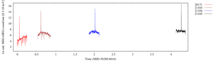
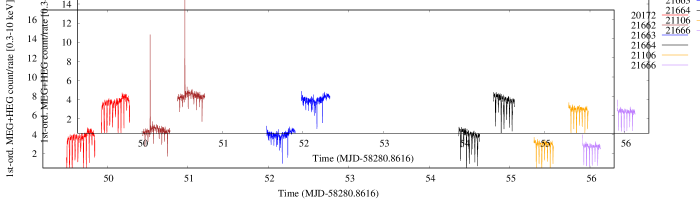
Figure 1: First-order MEG+HEG light curves of the observations in the 0.3-10 keV energy range. The bin time is 128 s.

We analyzed ten new observations of XB 1916-053 collected by the Chandra observatory in 2018 and the Swift/XRT observation (ObsID. 87248021) taken on 2017 July 30; furthermore, we reanalyzed the Chandra observation taken in 2004 August 7 (see Iaria et al. 2006).

The new Chandra observations were performed from 2018 June 11 to August 6 using the onboard High Energy Transmission Grating Spectrometer (HETGS) in timed graded mode; the detailed list of the observations is shown in Table 1. HETGS consists of two types of transmission gratings, the medium energy grating (MEG) and the high-energy grating (HEG). The HETGS provides high-resolution spectroscopy from 1.2 to 31 $\AA$ (0.4-10 keV) with a peak spectral resolution of $\lambda/\Delta\lambda\sim$1000 at 12 $\AA$ for first-order HEG. The dispersed spectra were recorded with an array of six charge-coupled devices (CCDs) that are part of the Advanced CCD Imaging Spectrometer-S.

We reprocessed the data using the FTOOLS ver. 6.26.1 and the CIAO ver. 4.11 packages. The brightness of the source required additional efforts to mitigate pileup issues. A 512 row subarray (the first row = 1) was applied during the observations, reducing the CCD frame time to 1.7 s. We ignored the zeroth-order events in our analysis focusing on the first-order HEG and MEG spectra. We reprocessed the data adopting a scale factor (width$\_$factor$\_$hetg) that multiplies the approximate one sigma width of the HEG/MEG mask in the cross-dispersion direction of 15, instead of the default value of 35, in order to avoid that HEG and MEG overlap in the Fe K region of the spectrum. We obtained HEG and MEG region widths of 33 and 44 pixels, respectively.

We applied barycentric correction to the events adopting the source coordinated obtained by Iaria et al. (2006) and extracted the light curve for each observation retaining only the first-order MEG and HEG data in the 0.3-10 keV energy range. We show the light curves of the ten observations in Fig. 1. During the persistent emission, the observations taken in 2018 June (ObsID. 20171, 21103, 21104, 21105) have a higher count rate than those taken in July-August (ObsID. 20172, 21662, 21663, 21664, 21106, 21666). Observations 21103, 21104, and 21105 show a count rate close to 7 c s^-1 (20171 shows a count rate of 5 c s^-1); observations 20172, 21662, 21663, and 21664 show a count rate of 4.5 c s^-1; and observations 21106 and 21666 show a count rate of 3 c s^-1. We observed five type I X-ray bursts, four during the high-flux state and one when the flux of the source dropped below 5 c s^-1. Furthermore, the light curves corresponding to observations 21104 and 21105 (when XB 1916-056 showed a high flux) do not show dips, while the dipping activity is intense at lower fluxes. A similar behavior was observed during a long Suzaku observation of the source (see Gambino et al. 2019).

XB 1916-053 was monitored by the X-Ray Telescope (XRT; Burrows et al. 2005) on board the Swift Observatory (Gehrels et al. 2004). We analyzed the Swift/XRT observation 87248021 taken on 2017 July 30 10:54:17, with elapsed and exposure times of 87 ks and 8.9 ks, respectively. The observation was performed in photon counting (PC) mode. The data were locally reprocessed by the UK Swift Science Data Center using HEASOFT v6.26.1. We applied barycentric correction to the events using the ftool barycorr. Using XSELECT we extracted the source events in the 1-4 keV energy range adopting a circular region of 100$\arcsec$; the background events in the same energy range were extracted using a same size circular region free from the source. Finally, we applied the exposure-correction to the source and background-light curves and extracted the background-subtracted light curve using the ftools xrtlccorr and lcmath.

3 Updated orbital ephemeris of XB 1916-053

First, we filtered the light curves to exclude the type I X-ray bursts; then we selected the events in the 1-4 keV energy range to estimate the dip arrival times. We estimated one dip arrival time from the Chandra observations taken in June, one from those taken in July-August, and one from the XRT observation.

The light curves were folded adopting $P_{0}=$3000.6511 s as the orbital period. For the first dip arrival time we folded the light curve obtained from observation 20171, where the dips are the deepest, adopting a folding time $T_{fold}=$58281 MJD; to obtain the second we folded together the light curves of observations 20172, 21664, 21106, and 21666, adopting $T_{fold}=$58333.65 MJD. Finally, the XRT light curve was folded assuming $T_{fold}=$57965 MJD.

We fitted the dips with a simple model consisting of a step-and-ramp function, where the count rates before, during, and after the dip are constant and the intensity changes linearly during the dip transitions (see Iaria et al. 2015, for a description). We show the X-ray dip arrival times in Table 2.

Table 2: Journal of the estimated dip arrival times

Dip Time	Cycle	Delay (s)	Observation
(MJD;TDB)
57965.0004(2)	225800	$1062\pm 14$	Swift/XRT
58281.0075(2)	234899	$1155\pm 21$	1st ord. HEG+MEG
58333.65781(6)	236415	$1151\pm 8$	1st ord. HEG+MEG

Epoch of reference 50123.00873 MJD, orbital period 3000.6511 s.

To obtain the delays with respect to a constant period reference, we used the period $P_{0}=3000.6511$ s and reference epoch $T_{0}=50123.00873$ MJD. Hence, we added the three dip arrival times to the 27 values reported by Iaria et al. (2015).

We initially fitted the delays with a quadratic function $y(t)=a+bt+ct^{2}$, where $t$ is the time in days with respect to $T_{0}$, $a=\Delta T_{0}$ is the correction to $T_{0}$ in units of seconds, $b=\Delta P/P_{0}$ in units of s d^-1 with $\Delta P$ the correction to the orbital period, and $c=1/2\;\dot{P}/P_{0}$ in units of s d^-2 with $\dot{P}$ is the orbital period derivative. The quadratic form does not fit the data well, returning a $\chi^{2}({\rm{d.o.f.}})$ of 182(27). We show the delays (red points) and the quadratic curve (black curve) in the top panel of Fig. 2. The best-fit values of the parameters are shown in the second column of Table 3.

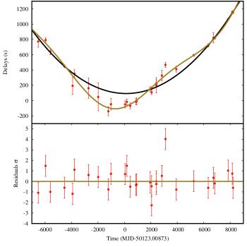
Figure 2: Top panel: Delays vs time (red points). The black curve is the best fit of the LQ function. The brown curve is the best fit of the LQS function. Bottom panel: Residuals in units of $\sigma$ vs time, corresponding to the LQS function

Table 3: Best-fit values of the functions adopted to fit the delays.

Parameters	LQ	LS	LQS
$a$ (s)	$93\pm 22$	$5495\pm 300$	$14\pm 14$
$b$ ($\times 10^{-3}$ s d-1)	$-4\pm 4$	$-408\pm 144$	$5\pm 3$
$c$ ($\times 10^{-5}$ s d-2)	$1.64\pm 0.07$	–	$1.82\pm 0.04$
$A$ (s)	–	$7343\pm 1380$	$130\pm 14$
$t_{\phi}$ (d)	–	$9826\pm 1795$	$1262\pm 133$
$P_{mod}$ (d)	–	73574 (fixed)	$9099\pm 302$
$\chi^{2}$(d.o.f.)	182(27)	132(26)	37(24)

Note — The reported errors are at 68% confidence level. The best-fit parameters of the delays are obtained using the functions LQ (column 2), LS (column 3), and LQS (column 4).

To improve the modeling of the delays we added a cubic term to the previous parabolic function, $y(t)=a+bt+ct^{2}+dt^{3}$, where $d$ is defined as $\ddot{P}/(6P_{0})$ and $\ddot{P}$ indicates the temporal second derivative of the orbital period. Fitting with this cubic function, we obtained a $\chi^{2}({\rm{d.o.f.}})$ of 129(26) with an F-test probability of chance improvement of only $3\times 10^{-3}$ with respect to the quadratic form (hereafter LQ function). We also tried to fit the delays using a linear plus a sinusoidal function (the LS function in Iaria et al. 2015), $y(t)=a+bt+A\sin\left[\frac{2\pi}{P_{mod}}(t-t_{\phi})\right],$ where $a$ and $b$ are defined as above, while $A$ and $P_{mod}$ are the amplitude in seconds and the period in days of the sinusoidal function, respectively. Finally, $t_{\phi}$ is the time in days referred to $T_{0}$ at which the sinusoidal function is null. Since the best-fit value of $P_{mod}$ is larger then the available time span, we fixed it to the best-fit value $P_{mod}=73574$ d. We found a $\chi^{2}({\rm{d.o.f.}})$ of 132(26); the best-fit parameters are shown in the third column of Table 3.

We added a quadratic term to the LS function to take into account the possible presence of an orbital period derivative $y(t)=a+bt+ct^{2}+A\sin\left[\frac{2\pi}{P_{mod}}(t-t_{\phi})\right]$ (hereafter LQS function). We obtained a value of $\chi^{2}({\rm{d.o.f.}})$ of 37(24) and an F-test probability of chance improvement with respect to the LQ function of $1.8\times 10^{-8}$. We show the best-fit curve of the LQS model (brown curve) and its relative residuals in units of sigma in the top and bottom panels of Fig. 2, respectively. The best-fit values are shown in the forth column of Table 3. The obtained best-fit values are compatible with the previous ones reported by Iaria et al. (2015).

The corresponding LQS ephemeris is

$$\begin{split}T_{dip}(N)={\rm MJD(TDB)}\;50\,123.0089(2)+\frac{3\,000.65129(8)}{86\,400}N+\\ +2.54(6)\times 10^{-13}N^{2}+\frac{A}{86\,400}\sin\left[\frac{2\pi}{P_{mod}}\left(t-t_{\phi}\right)\right],\end{split}$$ (1)

with $P_{mod}=9099\pm 302$ d ($24.9\pm 0.8$ yr), $t_{\phi}=1262\pm 133$ d, and $A=130\pm 14$ s. The corresponding orbital period derivative is $\dot{P}=1.46(3)\times 10^{-11}$ s s^-1. Our analysis suggests that a quadratic or a quadratic plus a cubic term do not adequately fit the delays, as already shown by Iaria et al. (2015).

We folded the 0.3-10 keV first-order MEG+HEG light curves obtained from the observations (type I X-ray bursts excluded), adopting the orbital period inferred by the LQS ephemeris and changing the reference time so that the dip falls at the orbital phase 0.5. The epoch-folded light curves are shown in Fig. 3.

Figure 3: First-order MEG+HEG folded light curves in the 0.3-10 keV energy range adopting the LQS ephemeris. An ad hoc phase shift of 0.5 is imposed. The label in the plot shows the correspondence between colors and observations. The blue dashed horizontal lines indicate the arbitrary count rate threshold of 3.5 c s^-1 and 5.5 c s^-1 adopted to select the four sets of observations (see text).

We distinguish four different sets of epoch-folded light curves at different count rates: the first set (hereafter set A) associated with observation 4584 has a persistent count rate higher than 10 c s^-1 (gold curve in Fig. 3); the folded curves of the second set (hereafter set B), have a persistent count rate between 6 and 8 c s^-1 and are associated with observations 21103, 21104, and 21105 (orange, blue, and magenta curve in Fig. 3); the third set of curves (hereafter set C) has a persistent count rate between 3.5 and 5.5 c s^-1 and is associated with observations 20171, 20172, 21662, 21663, and 21664 (black, red, brown, gray, and purple curve in Fig. 3); the fourth set (hereafter set D) shows a count rate close to 3.5 c s^-1 outside the dip associated with observations 21106 and 21666 (yellow and green curve in Fig. 3).

Table 4: List of the combined spectra

Combined first-order	Exp. time	ObsID.	Phase interval
HEG+MEG spectrum	(ks)		excluded
spectrum A	38.8	4584	0.45-0.60
spectrum B	67.3	21104
		21105
		21103	0.45-0.60
spectrum C	104.2	20171	0.40-0.65
		21662	0.45-0.60
		21663	0.55-0.66
		21664	0.40-0.70
		20172	0.40-0.65
spectrum D	31.4	21106	0.40-0.60
		21666	0.40-0.60

Table 5: Best-fit values of Model 1 and Model 2

Model	Component	Model 1a				Model 2b
		A	B	C	D	A	B	C	D
Constant	CHEG	$0.972\pm 0.006$	$0.970\pm 0.006$	$0.966\pm 0.006$	$0.956\pm 0.015$	$0.972\pm 0.006$	$0.969\pm 0.006$	$0.966\pm 0.006$	$0.956\pm 0.015$
Edge	E (keV)	–				0.871 (fixed)
	$\tau$	–				$0.14\pm 0.05$
TBabs	NHc	$0.56\pm 0.07$	$0.63\pm 0.08$	$0.53\pm 0.09$		$0.55\pm 0.04$	$0.60\pm 0.05$	$0.50\pm 0.05$
partcov	$f_{\rm cabs}$d	–				$>0.86$
Cabs	N${}_{{\rm H}_{\rm cabs}}$e	–				$19^{+7}_{-3}$	$14^{+5}_{-2}$	$17^{+6}_{-3}$	$10\pm 7$
zxipcf	N${}_{{\rm H}_{\xi}}$c	–				$19^{+7}_{-3}$	$14^{+5}_{-2}$	$17^{+6}_{-3}$	$10\pm 7$
	log($\xi$)	–				$4.33\pm 0.02$
	$f$	–				$>0.86$
	$z$ ($\times 10^{-3}$)	–				$1.3\pm 0.2$	$1.1\pm 0.2$	$1.1\pm 0.2$	$1.0^{+1.3}_{-1.6}$
nthcomp	$\Gamma$	$1.613\pm 0.012$	$1.721\pm 0.015$	$1.841\pm 0.015$	$1.80^{+0.02}_{-0.03}$	$1.620\pm 0.009$	$1.730\pm 0.013$	$1.848\pm 0.014$	$1.803^{+0.014}_{-0.010}$
	kTbb (keV)	$0.17\pm 0.05$				$0.16\pm 0.04$
	kTe (keV)	$2.9\pm 0.3$	$2.6\pm 0.2$	$3.8^{+1.4}_{-0.9}$	$3.3^{+4.9}_{-0.6}$	$3.2^{+0.5}_{-0.3}$	$2.6\pm 0.3$	$>3.6$	$>2.8$
	Norm ($\times 10^{-2}$)	$11.7\pm 1.3$	$10.9\pm 1.3$	$7.2\pm 1.0$	$4.8\pm 0.7$	$14.3\pm 1.0$	$12.8\pm 1.0$	$8.7\pm 0.8$	$5.4\pm 0.5$
	$\chi^{2}/dof$	4957/4553				3944/4542

• The associated errors are at 90% confidence level.

• Model 1 = Const*TBabs*nthcomp.

• Model 2 = Const*TBabs*(partcov*Cabs)*zxipcf*nthcomp.

• Equivalent hydrogen column density in units of 10²² atoms cm^-2.

• The value of the parameter is tied to the value of $f$.

• The value of the parameter is tied to the value of N${}_{{\rm H}_{\xi}}$.

4 Spectral analysis

We extracted the combined spectrum from each distinguished set, calling the spectra A, B, C, and D, using the CIAO script combine$\_$grating$\_$spectra and combining the corresponding first-order MEG and HEG spectra. Since our aim is the spectral analysis out of the dips, we excluded the orbital phases in which the dip falls when it is present. The excluded phases are shown in Table 4. Spectrum B was obtained by excluding the phases between 0.45 and 0.6 from observation 21103; the other two observations do not show dipping activity, and we included all the phases. We rebinned the resulting first-order MEG and HEG spectra of selections A, B, C, and D to have at least 250 counts per energy channel. Such a large rebinning could affect the spectroscopic study of narrow discrete features because it risks losing energy resolution. However, we tried to fit these spectra using a rebinning so as to have 25 counts per energy channel, verifying that we obtained results that are compatible with those reported in the following. For the analysis we adopted the energy ranges 0.7-7 keV and 0.9-10 keV for the first-order MEG and HEG spectrum, respectively.

To fit the spectra we used XSPEC v12.10.1p; we adopted the cosmic abundances and the cross sections derived by Wilms et al. (2000) and Verner et al. (1996a), respectively. To take into account the interstellar absorption we adopted the Tübingen-Boulder model (TBabs in XSPEC). We fitted the spectrum using a Comptonized component (nthcomp in XSPEC; Zdziarski et al. 1996). Finally, we added a constant to take into account the different normalizations of the two instruments. The initial model, called Model 1, is defined as

$$\texttt{Model 1}=\textsc{Const*TBabs*nthcomp}.$$

We fixed at 0 the value of the parameter inp$\_$type in nthcomp, assuming the seed-photon spectrum injected in the Comptonizing cloud to be a blackbody. The spectra A, B, C, and D were fitted simultaneously. The value of the seed-photon temperature k$T_{bb}$ was tied at the same value in each spectrum and, finally, the value of the interstellar equivalent neutral hydrogen column density was tied at the same value in spectra C and D.

We show the unfolded spectra and the residuals in the left panels of Fig. 4. The best-fit parameters are shown in Table 5. Strong residuals compatible with absorption lines are visible at 1 keV, 1.47 keV, 2 keV, 2.62 keV, and 6.97 keV. Furthermore, below 0.9 keV there is a clear excess in the residuals.

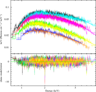
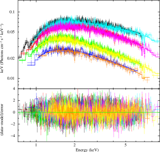
Figure 4: Unfolded spectrum and residuals adopting Model 1 (left panels) and Model 2 (right panels). The black, red, green, and blue data correspond to the first-order MEG of spectra A, B, C, and D, respectively. The cyan, purple, yellow, and orange data correspond to first-order HEG spectrum of spectra A, B, C, and D, respectively. The prominent absorption lines in residuals of Model 1 (bottom left panel) are associated with the presence of Ne x, Mg xii, Si xiv, S xvi, and Fe xxvi ions.

Table 6: Identified Gaussian absorption lines.

Component	Spectrum A	Spectrum B	Spectrum C	Spectrum D
	Ne x K$\alpha$ 1s-2p (1.0218 keV)
E (keV)	$1.020\pm 0.002$	$1.014\pm 0.009$	$1.019^{+0.009}_{-0.019}$	–
$\sigma$ (eV)	$<2.0$	$<17$	$<31$	–
Intensitya	$-8\pm 2$	$-8\pm 5$	$>-6$	–
Eq. widthb	$-1.8\pm 0.5$	$-2.1\pm 0.8$	$-1.1\pm 0.8$	–
Bin sizec (eV)	6	10	7	–
	Mg xii K$\alpha$ 1s-2p (1.4723 keV)
E (keV)	$1.4715\pm 0.0004$	$1.4720\pm 0.0005$	$1.4720^{+0.0005}_{-0.0009}$	–
$\sigma$ (eV)	$1.0\pm 0.5$	$<1.8$	$<2.2$	–
Intensity	$-5.9\pm 0.7$	$-5.0\pm 1.0$	$-2.9\pm 0.6$	–
Eq. width	$-1.3\pm 0.2$	$-1.1\pm 0.2$	$-1.1\pm 0.2$	–
Bin size (eV)	2	2	2	–
	Si xiv K$\alpha$ 1s-2p (2.0055 keV)
E (keV)	$2.0044\pm 0.0004$	$2.0040^{+0.0007}_{-0.0002}$	$2.0039\pm 0.0010$	$2.005^{+0.003}_{-0.014}$
$\sigma$ (eV)	$1.4^{+0.5}_{-1.2}$	$0.6^{+1.1}_{-0.6}$	$3.4^{+0.7}_{-1.2}$	$<29$
Intensity	$-9.0\pm 0.8$	$-6.7\pm 0.8$	$-5.2\pm 0.8$	$-2.2\pm 1.5$
Eq. width	$-2.6\pm 0.3$	$-2.2\pm 0.2$	$-2.8\pm 0.3$	$-1.8\pm 0.6$
Bin size (eV)	3	3	3	20
	Si xiv K$\alpha$ 1s-3p (2.376 keV)
E (keV)	$2.372\pm 0.002$	–	–	–
$\sigma$ (eV)	$1.3^{+3.6}_{-1.3}$	–	–	–
Intensity	$-6\pm 2$	–	–	–
Eq. width	$-1.9\pm 0.5$	–	–	–
Bin size (eV)	9	–	–	–
	S xvi K$\alpha$ 1s-2p (2.6217 keV)
E (keV)	$2.6157^{+0.0002}_{-0.0027}$	$2.621^{+0.002}_{-0.008}$	$2.617^{+0.006}_{-0.004}$	–
$\sigma$ (eV)	$<3.0$	$7\pm 6$	$5\pm 5$	–
Intensity	$-9\pm 2$	$-7\pm 4$	$-3.3\pm 1.5$	–
Eq. width	$-3.4\pm 0.7$	$-3.3\pm 0.9$	$-2.7\pm 0.7$	–
Bin size (eV)	8	8	8	–
	Ca xx K$\alpha$ 1s-2p (4.1050 keV)
E (keV)	$4.102\pm 0.006$	–	–	–
$\sigma$ (eV)	$8^{+7}_{-8}$	–	–	–
Intensity	$-6\pm 2$	–	–	–
Eq. width	$-2.9^{+0.3}_{-2.5}$	–	–	–
Bin size (eV)	20	–	–	–
	Fe xxvi K$\alpha$ 1s-2p (6.9662 keV)
E (keV)	$6.98^{+0.04}_{-0.09}$	$6.956^{+0.028}_{-0.003}$	$6.96\pm 0.04$	–
$\sigma$ (eV)	$<42$	$<60$	$<35$	–
Intensity	$-16\pm 6$	$-18\pm 6$	$-7\pm 2$	–
Eq. width	$-13.1^{+1.0}_{-26.3}$	$-33\pm 7$	$-43^{+23}_{-4}$	–
Bin size (eV)	100	100	120	–

• The associated errors are at 68% confidence level.

• The line intensity is in units of $\times 10^{-5}$ photons cm^-2 s^-1.

• The equivalent width is in units of eV.

• The size of the energy channel at the detected lines is estimated from MEG spectra except for the Ca xx and Fe xxvi lines.

We fitted each observed absorption line with a Gaussian component. The energies, widths, intensities, and equivalent widths of each identified line are shown in Table 6 for each spectrum. We detected the absorption lines associated with the presence of ions of Ne x, Mg xii, Si xiv, S xvi, Ca xx, and Fe xxvi. The line associated with the Ca xx ions is detected only in spectrum A. Spectrum D only showed the line associated with Si xiv, probably because of the low flux of the spectrum. For the sake of clarity the sizes of the energy channels at which we identified the absorption lines are shown in Table 6.

To account for the presence of the prominent absorption lines, to the continuum of Model 1 we added the multiplicative component zxipcf, which takes into account a partial covering of ionized absorbing material. The component reproduces the absorption from photoionized matter illuminated by a power-law source with spectral index $\Gamma=2.2$, and it assumes that the photoionized absorber has a microturbulent velocity of 200 km s^-1 (see Reeves et al. 2008; Miller et al. 2007, for applications to AGN and Seyfert 1 galaxies). Recently, this component was adopted to fit the absorbing features in the Fe-K region associated with highly ionized matter surrounding the eclipsing NS-LMXB AX J1745.6-2901 (Ponti et al. 2015), the dipping source XB 1916-053 (Gambino et al. 2019), and the eclipsing source MXB 1659-298 (Iaria et al. 2019). The parameters of this component are N${}_{{\rm H}_{\xi}}$, log($\xi$), $f$, and $z$: N${}_{{\rm H}_{\xi}}$ describes the equivalent hydrogen column density associated with the ionized absorber, log($\xi$) describes the ionization degree of the absorbing material, $f$ is a dimensionless covering fraction of the emitting region, and $z$ is the redshift associated with the absorption features. The parameter $\xi$ is defined as $\xi=L_{x}/(n_{H}r^{2})$, where $L_{x}$ is the X-ray luminosity incident on the absorbing material, $r$ is the distance of the absorber from the X-ray source, and $n_{H}$ is the hydrogen atom density of the ionized absorber.

To take into account that the ionized absorber can scatter the radiation out of the line of sight via Thomson or Compton scattering, we added the multiplicative component cabs to the model. The only parameter of the component cabs is $N_{H_{\rm cabs}}$, which describes the equivalent hydrogen column density associated with the scattering cloud. Finally, to account for a partial covering of the scattering material, we multiplied cabs by the component partcov. This is a convolution model that allows us to convert an absorption component into a partially covering absorption component, quantified by the parameter $f_{\rm cabs}$. In order to make the model self-consistent, we tied $f_{\rm cabs}$ to the parameter $f$ of the ionized absorber. Moreover, we linked the equivalent hydrogen column density parameter of the scattering cloud, $N_{H_{\rm cabs}}$, to the value of the equivalent hydrogen column density of the ionized absorber, N${}_{{\rm H}_{\xi}}$. While fitting simultaneously spectra A, B, C and D, we imposed $f$, log($\xi$), and the seed-photon temperature to assume the same value for each spectrum. The model closely fits the absorption lines; however, the presence of an excess in the residuals below 0.9 persists. For this reason we added an absorption edge with the energy threshold fixed at 0.871 keV to account for the presence of O viii ions along the line of sight, recently observed by Gambino et al. (2019) analyzing the Suzaku spectra of the source.

The adopted model, hereafter called Model 2, is defined as

$$\begin{split}\texttt{Model 2}=\textsc{Const*Edge*TBabs*(partcov*cabs)*}\\ \textsc{{zxipcf*nthcomp}}.\end{split}$$

The addition of zxipcf and the absorption edge improves the fits, with a $\chi^{2}$(d.o.f.) of 3944(4542) and a $\Delta\chi^{2}$ of 1013 with respect to Model 1. We show the best-fit values in Table 5 for each spectrum. The unfolded spectra and the corresponding residuals are shown in the right panels of Fig. 4; the residuals associated with the absorption lines and the excess below 0.9 keV observed adopting Model 1 are now absent.

We found that the ionized absorber covers more than 86% of the emitting source and the ionization parameter log($\xi$) is $4.33\pm 0.02$. The equivalent hydrogen column density associated with the ionized absorber N${}_{{\rm H}_{\xi}}$ is $(19^{+7}_{-3})\times 10^{22}$, $(14^{+5}_{-2})\times 10^{22}$, $(17^{+6}_{-3})\times 10^{22}$, and $(10\pm 7)\times 10^{22}$ cm^-2 for spectra A, B, C, and D, respectively. Furthermore, we observed a similar redshift value for each spectrum (between $1.0\times 10^{-3}$ and $1.3\times 10^{-3}$).

The $\Gamma$ parameter of nthcomp goes from 1.6 for spectrum A to 1.8 for spectrum C and D, indicating that the spectral shape softens going from spectrum A to spectrum D. The electron temperature of the Comptonizing cloud is compatible with 3-4 keV for all the spectra even if it is not well constrained for spectra C and D, while the seed-photon temperature is $0.16\pm 0.04$ keV.

Finally, the best-fit value of the optical depth of the absorption edge is $0.14\pm 0.05$ and the equivalent hydrogen column density of the interstellar matter is compatible with $0.5\times 10^{22}$ cm^-2 for each spectrum.

Assuming a distance to the source of 8.9 kpc (Galloway et al. 2008), the unabsorbed luminosity in the 0.1-100 keV energy range is $1.46\times 10^{37}$ erg s^-1, $1.0\times 10^{37}$ erg s^-1, $0.67\times 10^{37}$ erg s^-1, and $0.41\times 10^{37}$ erg s^-1 for A, B, C, and D, respectively.

5 Spectral analysis of the dips

To analyze the average spectrum during the dips we extracted the events from observations 20171, 20172, 21106, 21662, 21663, 21664, and 21666. The dip events were selected from observation 20171 taking into account the good times intervals (GTIs) obtained from the first-order MEG+HEG light curve in the 0.3-10 keV energy range where the count rate was lower than 3 c s^-1. Similarly, we used the threshold of 2 c s^-1 for ObsID. 20172, 2.4 c s^-1 for ObsID. 21662, 2 c s^-1 for ObsID. 21663 and 21664, 1.5 c s^-1 for ObsID. 21106, and 1.1 c s^-1 for ObsID. 21666. We extracted the first-order HEG and MEG spectrum from each observation and combined them using the CIAO script combine$\_$grating$\_$spectra. Each spectrum was then grouped to have at least 100 counts per energy channel; the resulting spectrum has an exposure time of 9.5 ks. The energy range adopted for the spectral analysis is 0.9-7 keV and 1-9 keV for MEG and HEG, respectively.

We fitted the spectrum adopting Model 2; however, we excluded the edge component because of the low flux of the spectrum. does not allow us to constrain it. We kept the photon-index value, the electron temperature, and the seed-photon temperature of the nthcomp component fixed to 1.8, 4.3 keV, and 0.16 keV, respectively. We did this so that the dip-spectrum was extracted from the observations belonging to set C and D, under the assumption that the spectral shape of the continuum emission is similar both inside and outside the dips.

We show the best-fit parameters in Table 7; the unfolded spectrum and the corresponding residuals are shown in Fig. 5.

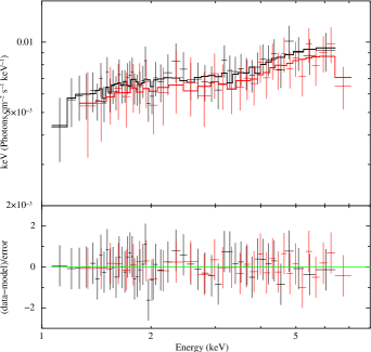
Figure 5: Unfolded spectrum and residuals of the dip spectrum adopting Model 2. The black and red data correspond to the first-order MEG and HEG spectra, respectively.

Table 7: Best-fit parameters of the spectrum during the dip.

		Dip spectrum
Model	Component
Constant	CHEG	$0.92\pm 0.08$
partcov	$f_{\rm cabs}$a	$>0.68$
cabs	N${}_{\rm H_{\rm cabs}}$b ($\times 10^{22}$)	$61^{+56}_{-10}$
zxipcf	N${{}_{\rm H}}_{\xi}$ ($\times 10^{22}$)	$61^{+56}_{-10}$
	log($\xi$)	$2.8^{+0.2}_{-0.4}$
	$f$	$>0.68$
	Redshift	0 (fixed)
TBabs	NH($\times 10^{22}$)	$0.9\pm 0.2$
nthcomp	$\Gamma$	1.8 (fixed)
	kTbb (keV)	0.16 (fixed)
	kTe (keV)	4.3 (fixed)
	Norm ($\times 10^{-2}$)	$7.2\pm 1.4$
	$\chi^{2}/dof$	18.3/76

• The value of the parameter is tied to the value of $f$.

• The value of the parameter is tied to the value of N${}_{{\rm H}_{\xi}}$.

We found that during the dip the ionized absorber is characterized by log($\xi$)$=2.8^{+0.2}_{-0.4}$, suggesting a low ionization of the absorber. The equivalent hydrogen column density N${{}_{\rm H}}_{\xi}$ associated with the ionized absorber is $(61^{+56}_{-10})\times 10^{22}$ cm^-2, which is larger than the values obtained during the persistent emission by a factor between 3 and 6.

The covering fraction is $>0.68$, compatible with the values obtained for spectra A, B, C, and D. The equivalent hydrogen column density associated with the interstellar matter is $(0.9\pm 0.2)\times 10^{22}$ cm^-2. This value is larger than the observed value during the persistent emission. We cannot exclude that a partial contribution to this value comes from local neutral hydrogen in the hypothesis that during the dip the absorber is composed of neutral and mildly ionized matter.

Finally, the 0.1-100 keV unabsorbed luminosity, assuming a distance to the source of 9 kpc, is $0.57\times 10^{37}$ erg s^-1.

6 Discussion

From the analysis of the Chandra and Swift/XRT observations we inferred three new dip arrival times that, added to the previous 27 reported by Iaria et al. (2015), allowed us to update the orbital ephemeris of XB 1916-053 by extending the temporal baseline from 36 to 40 years. The largest baseline excludes some solutions previously plausible with the available data, such as the LQ ephemeris shown by Iaria et al. (2015). We find that the LQS ephemeris better models the dip arrival times, improving the constraints on the orbital period derivative and the sinusoidal modulation. The orbital period derivative is $\dot{P}=1.46(3)\times 10^{-11}$ s s^-1 and the sinusoidal modulation has a period of $P_{\rm{mod}}=9099\pm 302$ d.

Iaria et al. (2015) discussed that such a large orbital period derivative can be explained only assuming that the mass transfer rate from the CS to the NS is highly non-conservative. The authors estimated that more that 90% of the mass transfer rate from the CS is lost by the system, the mass ratio $q=m_{2}/m_{1}$ ($m_{1}$ and $m_{2}$ are the NS and CS mass in units of solar masses) is close to 0.013 and the NS mass should be larger than 2.1 M_⊙.

Here we show that the conclusions of Iaria et al. (2015) were strongly constrained by the hypothesis that the matter leaves the system from the inner Lagrangian point. To discuss this point we have to estimate the mass ratio $q$ of XB 1916-053.

6.1 Mass ratio $q$ of XB 1916-053

XB 1916-053 shows a superhump period $P_{sh}$ (Chou et al. 2001) and a negative superhump period, also called infrahump period, $P_{ih}$ (Retter et al. 2002; Hu et al. 2008). Chou et al. (2001) discussed that the optical modulation close to 3028 s is likely caused by the coupling of the orbital motion with a 3.9-day disk apsidal precession period, like the superhumps in SU UMa-type dwarf novae, obtaining from this assumption $q\simeq 0.022$, while Hu et al. (2008) discussed the infrahump period of 2979.3(1.1) s detected by Retter et al. (2002) as being due to the nodal precession period of the tilted accretion disk, and finding $q\simeq 0.045$. Considering that the orbital period of the system is close to 3000.66 s, the apsidal precession period of the disk should be 3.9087(8) d, while the retrograde nodal precession period 4.86 d. However, the reported values of $q$ do not depict a self-consistent scenario. We show below that the value of $q=0.048$ is consistent with the detected values of $P_{sh}$ and $P_{ih}$ only assuming an outer radius of the disk truncated at a 3:1 resonance.

Hirose & Osaki (1990), performing hydrodynamic simulations of accretion disks to study the superhump phenomenon in SU UMa stars, showed that the apsidal precession frequency $\omega_{p}$ can be written as $\omega_{p}/\omega_{\rm orb}=Z(r)q/(1+q)^{1/2}$, where

$$\begin{split}Z(r)=\frac{1}{2}\frac{1}{r^{1/2}}\frac{d}{dr}\left[r^{2}\frac{d}{dr}B_{0}(r)\right],\end{split}$$

and

$$\begin{split}B_{0}(r)=\frac{1}{2}b_{1/2}^{(0)}=1+\frac{1}{4}r^{2}+\frac{9}{64}r^{4}+...,\end{split}$$

which is the Laplace coefficient of order 0 in celestial mechanics (see Brouwer & Clemence 1961, chapter 15, eq. 42) and $r$ is the ratio of the accretion disk radius $r_{\rm disk}$ to the orbital separation $a$. Combining the expressions we find that

$$\begin{split}\frac{\omega_{p}}{\omega_{\rm orb}}=\frac{q}{(1+q)^{1/2}}r^{3/2}\left[0.75+\frac{45}{32}r^{2}\right].\end{split}$$ (2)

Hirose & Osaki (1990) demonstrated that the tidal instability in the accretion disks is caused by the resonance between the particle orbits in the disk and the companion star with a 3:1 period ratio in SU UMa dwarf novae. Since $r=r_{\rm disk}/a$ can be expressed by the equation

$$\begin{split}\frac{r_{\rm disk}}{a}=\frac{R_{jk}}{a}=\left(\frac{j-k}{j}\right)^{2/3}(1+q)^{-1/3},\end{split}$$ (3)

with $j=3$ and $k=2$ for a 3:1 resonance (see Frank et al. 2002, eq. 5.125), we can combine the two last equations to obtain

$$\begin{split}\frac{\omega_{p}}{\omega_{\rm orb}}=\frac{1}{3}\frac{q}{1+q}[0.75+0.325(1+q)^{-2/3}];\end{split}$$ (4)

using the value $\omega_{p}/\omega_{\rm orb}\simeq 0.0089$ inferred by Chou et al. (2001) we find $q\simeq 0.0256$.

However, Hirose & Osaki (1990) estimated the apsidal precession period of the disk taking into account only the dynamical effects of the matter. Lubow (1991a, b, 1992) showed that the apsidal precession rate $\omega$ for an eccentric disk is given by three terms $\omega=\omega_{\rm dyn}+\omega_{\rm press}+\omega_{\rm tr}$, where $\omega_{\rm dyn}$ is the dynamical precession frequency discussed by Hirose & Osaki (1990) and shown above, $\omega_{\rm press}$ is a term due to the pressure, and $\omega_{\rm tr}$ is a transient term related to the time-derivative of the mode giving rise to the dynamical precession that can be neglected in steady state. Since XB 1916-053 is a persistent source that does not show outburst, and since Callanan et al. (1995) verified the stability of the optical period over seven years, we do not consider the last term as we assume that the disk precesses in a steady state.

Lubow (1992) showed that the pressure term can be written as $\omega_{\rm press}$=$-k^{2}c_{s}^{2}/(2\Omega)$, where $k$ is the radial wavenumber of the mode, $c_{s}$ the sound speed of the gas, and $\Omega$ is the frequency of a particle in the disk at a given radius. The negative sign is due to the pressure term associated with a spiral arm in the disk, which acts in the opposite sense with respect to the dynamical term. For a spiral wave, the pitch angle $\theta$ is related to $k$ by the relation $\tan\theta=(kR)^{-1}$, where $R$ is the distance from the central source.

Pearson (2006), considering a 3:1 resonance and adopting eq. 3, expressed the term associated with the pressure of the spiral wave $\omega_{\rm press}$ as

$$\begin{split}\frac{\omega_{\rm press}}{\omega_{\rm orb}}=-\frac{j^{1/3}}{2}(1+q)^{2/3}\left(\frac{c_{s}}{\omega_{\rm orb}\;a}\tan^{-1}\theta\right)^{2}=-j^{1/3}\eta_{A}(1+q)^{2/3},\end{split}$$ (5)

where $a$ is the orbital separation, $j=3$, and $\eta_{A}=0.5[c_{s}/(\omega_{\rm orb}\;a)]^{2}\tan^{-2}\theta$. We combined eqs. 4 and 5 and obtained

$$\begin{split}\frac{\omega}{\omega_{\rm orb}}=\frac{1}{3}\frac{q}{1+q}[0.75+0.325(1+q)^{-2/3}]-3^{1/3}\eta_{A}(1+q)^{2/3},\end{split}$$ (6)

where $\omega$ is now the apsidal precession frequency of the disk taking into account the pressure term.

Hu et al. (2008), assuming a 3:1 resonance, inferred a value of $q\simeq 0.045$ based on the negative superhump with a period of 2979.3 s observed by Retter et al. (2002), and interpreted as the beat period between the orbital period and the 4.86 d nodal precession period of the disk. The value of $q\simeq 0.045$ was obtained from the expression proposed by Larwood et al. (1996) and Montgomery (2009)

$$\begin{split}\frac{\omega_{n}}{\omega_{\rm k}}=-\frac{15}{32}qr^{3}\cos\delta,\end{split}$$ (7)

where $\omega_{n}$ is the angular frequency associated with the nodal precession of the disk, $\omega_{k}$ is the Keplerian frequency of the matter at a given radius $r$ of the accretion disk that is defined in units of orbital separation $a$, and the angle $\delta$ describes the orbit of the CS with respect to the NS. For $\delta\simeq 0$ the orbits of the two bodies are coplanar (Papaloizou & Terquem 1995). The minus sign is present because the nodal frequency is retrograde with respect to the orbital frequency (see Fig. 6.18 in Hellier 2001).

Rewriting the Keplerian frequency in the known form $\omega_{k}=(GM_{1}/R^{3})^{1/2}$ and combining it with Kepler’s third law $a^{3}=GM_{1}(1+q)/\omega_{orb}^{2}$ we find $\omega_{k}=\omega_{orb}(1+q)^{-1/2}r^{-3/2}$. We combined the last expression with eq. 7, obtaining

$$\begin{split}\frac{\omega_{n}}{\omega_{\rm orb}}=-\frac{15}{32}q(1+q)^{-1/2}r^{3/2}\cos\delta.\end{split}$$ (8)

Assuming that $r=r_{disk}/a$ (the same assumption made by Hu et al. 2008) and combining the last equation with eq. 3 for a 3:1 resonance, we infer

$$\begin{split}\frac{\omega_{n}}{\omega_{\rm orb}}=-\frac{5}{32}\frac{q}{1+q}\cos\delta.\end{split}$$ (9)

Because $\omega_{n}/\omega_{orb}\simeq 7.146\times 10^{-3}$, we adopt the nodal period of 4.86 days and find that $q\simeq 0.048$ for $\cos\delta\simeq 1$.

We show in Fig. 6

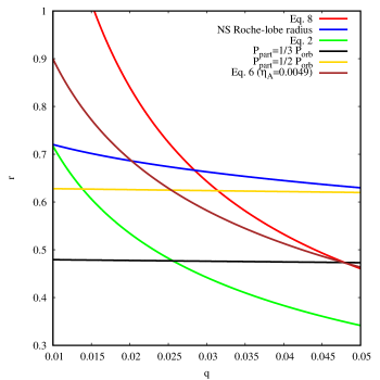
Figure 6: Characteristic radii of XB 1916-053 in units of orbital separation vs the mass ratio q. Show are the NS Roche-lobe radius (blue curve), the radius of the disk at which a 2:1 and 3:1 resonance could occur (yellow and black curves), the radius associated with the apsidal rate of the disk for a 3:1 resonance without and with the pressure term due to the presence of a spiral wave in the disk (green and brown curve), and the radius associated with the nodal precession period for a 3:1 resonance (red curve).

the Roche-lobe radius of the NS as a function of $q$ (blue curve), the outer radius of the accretion disk for a 2:1 resonance (yellow curve) and for a 3:1 resonance (black curve). The green curve represents the outer radius of the disk adopting the value of $\omega/\omega_{\rm orb}\simeq 8.9\times 10^{-3}$ obtained by Chou et al. (2001), who neglect the pressure term due to the spiral wave in the apsidal precession rate (see eq. 4). The red curve represents the outer radius of the disk assuming a nodal precession of 4.86 days obtained from eq. 9. All the radii are in units of orbital separation $a$.

Initially, we note that the green and red curve do not have intersections that exclude any self-consistent scenario; in other words, the outer radius of the disk estimated from the observed apsidal precession period is not compatible with that obtained from the observed nodal precession period if we ignore the pressure term. Taking into account $\omega_{\rm press}$, the outer radius of the disk obtained from the apsidal precession period can intersect the red curve. It is possible to obtain a pair of $r$ and $q$ values for a 3:1 resonance assuming that the parameter $\eta_{A}\simeq 0.0049$. For that value we find $q\simeq 0.048$ and an outer disk radius $r\simeq 0.474$ in units of orbital separation. It could be possible a solution for a 2:1 resonance for which $q\simeq 0.0315$, $r\simeq 0.62$, and $\eta_{A}\simeq 0.0089$; however, since the truncation radius of the disk due to the tidal interaction with the CS is $r_{T}=R_{T}/a=0.6/(1+q)$ (for $q$ between 0.03 and 1; Paczynski 1977), we obtain $r>r_{T}$, making the solution unrealistic.

A further indication that the mass ratio $q$ could be close to 0.048 is given by the empirical expressions inferred for the CVs, in which the period excess $\epsilon$ depends on $q$. Using the values of the superhump period $P_{\rm sh}=3027.5510(52)$ s and the orbital period $P_{\rm orb}=3000.6508(9)$ (see Table 1 in Retter et al. 2002, and references therein) we can define the period excess as

$$\begin{split}\epsilon=\frac{P_{\rm sh}-P_{\rm orb}}{P_{\rm orb}}=(8.965\pm 0.002)\times 10^{-3}.\end{split}$$ (10)

Using the empirical form $\epsilon=0.18q+0.29^{2}$ (Patterson et al. 2005) we obtain $q\simeq 0.045$. Goodchild & Ogilvie (2006) inferred $\epsilon=0.2076(3)q-4.1(6)\times 10^{-4}$, where the small offset from the origin is due to pressure-induced retrograde precession of a stable eccentric mode in systems with very low $q$. Using the last relation we infer that $q=0.0452\pm 0.0004$.

We obtain $q\simeq 0.048$ for

$$\begin{split}\eta_{A}=\frac{1}{2}\left(\frac{c_{s}}{\omega_{\rm orb}\;a}\right)^{2}\tan^{-2}\theta=0.0049.\end{split}$$ (11)

Lubow (1992) gave a range of 0.01-0.05 for the normalized speed of sound, $c_{s}/(\omega_{\rm orb}\;a),$ and inferred that for a tightly wrapped spiral arm the pitch angle $\theta$ is between 5.7^∘ and 31^∘. We show in Fig. 7 that for $\eta_{A}\simeq 0.0049$ this condition

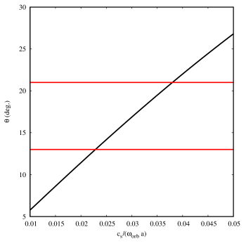
Figure 7: Pitch angle of the spiral wave vs the normalized sound of speed (black curve). The red horizontal lines correspond to the angles of pitch between 13^∘ and 21^∘, as obtained by Montgomery (2001) from simulations.

is verified, and we obtain that the pitch angle is between 5.8^∘ and 26.7^∘. From simulations Montgomery (2001) restricted the range of the pitch angle between 13^∘ and 21^∘; these values restrict the range of the normalized sound of speed between 0.023 and 0.038. Using Kepler’s third law and assuming $q=0.048$ we obtain that the sound speed $c_{s}$ is between $15.2m_{1}^{1/3}$ km s^-1 and $25.2m_{1}^{1/3}$ km s^-1. This range of values is compatible with a disk temperature in the outer region between $3\times 10^{4}$ K and $7\times 10^{4}$ K (see eq. 2.21 in Frank et al. 2002), which is compatible with the results obtained by Nelemans et al. (2006) from the analysis of the optical band of XB 1916-053. The authors found that a LTE model consisting of pure helium plus overabundant nitrogen closely fits the observed spectrum finding that the model has a temperature of $\sim 3\times 10^{4}$ K.

6.2 Neutron star mass $m_{1}$

Assuming that the CS fills its Roche lobe, we can obtain an indication of the NS mass. The CS is a degenerate star and its radius $R_{2}$ is given by $R_{2}/R_{\odot}=0.0126(1+X)^{5/3}m_{2}^{-1/3}$, where $X$ is the fraction of hydrogen in the star. This equation has to be corrected for the thermal bloating factor $b_{f}\geq 1$, which is the ratio of the CS radius to the radius of a star with the same mass and composition; this star is completely degenerate and supported only by the Fermi pressure of the electrons. Adopting the Roche-lobe prescription of Eggleton (1983), using Kepler’s third law and imposing that $R_{\rm l2}=b_{f}R_{2}$, where $R_{\rm l2}$ is the Roche-lobe radius of the CS, we obtain

$$\begin{split}m_{1}=14.17\;q^{-1/2}(1+q)^{-1/2}\left[\frac{0.49\;q^{2/3}}{0.6q^{2/3}+\ln(1+q^{1/3})}\right]^{-3/2}\\ P^{-1}(1+X)^{5/2}b_{f}^{3/2},\end{split}$$ (12)

where $P$ is the orbital period in seconds.

Heinke et al. (2013) inferred $X\sim 0.14$ for a NS mass of 1.4 M_⊙, compatible with the measurements of Nelemans et al. (2006). We can predict how $X$ varies with respect to $m_{1}$. Even though the CS is almost a pure helium dwarf, the small percentage of hydrogen that can be transferred onto the NS via Roche-lobe accretion can significantly change the energy released due to hydrogen’s larger energy release per nucleon (energy released per nucleon $Q_{\rm nuc}=1.6+4.0X$ MeV nucleon^-1; Cumming 2003). Galloway et al. (2008), using RXTE data, measured the ratio $\alpha$ of burst to persistent flux between two consecutive type I X-ray bursts temporally spaced by 6.3 hours obtaining $\alpha=78.8\pm 0.3$. We rewrite eq. 6 shown by Galloway et al. (2008) as

$$\begin{split}\alpha=34.57\;m_{1}(0.4+X)^{-1},\end{split}$$ (13)

in which we assumed a NS radius of 10 km. Adopting $\alpha=78.8\pm 0.3$ we find that $X$ is 0.21, 0.3, and 0.39 for a NS mass of 1.4, 1.6, and 1.8 M_⊙ respectively, while for a NS mass of 2.1 M_⊙ we find that $X\simeq 0.52$, in contrast with the pure helium dwarf nature of the CS. Furthermore, assuming an orbital period value $P=3000.66$ s and a mass ratio $q=0.048$, and combining Eqs. 12 and 13, we find

$$\begin{split}b_{f}=m_{1}^{2/3}(0.376+0.275m_{1})^{-5/3}.\end{split}$$ (14)

We obtain that $b_{f}$ is 1.97, 1.92, and 1.86 for a NS mass of 1.4, 1.6, and 1.8 M_⊙, respectively. In the following we explore the NS mass between 1.4 and 1.8 M_⊙ in order to have a fraction of hydrogen $X$ in the CS lower than 0.4.

Finally, we can express $m_{2}$ from eq. 12 remembering that $m_{1}=m_{2}q^{-1}$. We find

$$\begin{split}m_{2}=41.31\left(\frac{q}{1+q}\right)^{1/2}[0.6+q^{-2/3}\ln(1+q^{1/3})]^{3/2}\\ P^{-1}(1+X)^{5/2}b_{f}^{3/2}.\end{split}$$ (15)

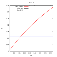
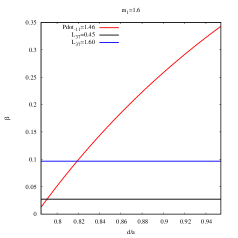
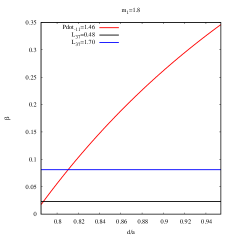
Figure 8: Constraint of the matter-ejection point position and $\beta$ for $q=0.048$. The left, middle, and right panels describe the constraints for $m_{1}$ values 1.4, 1.6, and 1.8 M_⊙. The red curve represents the orbital period derivative of $1.46\times 10^{-11}$ s s^-1 for the pairs $\beta$-$d/a$. The black and blue horizontal lines represent the minimum and maximum luminosity of the source during the observations. The minimum and maximum value of $d/a$ correspond to the inner Lagrangian point and the CS position with respect to the center of mass. The observed luminosities suggest that the mass transfer is highly non-conservative and that the ejected matter leaves the system close to the inner Lagrangian point.

6.3 Orbital period derivative and luminosity of XB 1916-053

Since XB 1916-053 has an orbital period close to 50 min we assume that the angular momentum lost via magnetic braking is negligible with respect to the angular momentum lost via gravitational waves. Combining eqs. 1, 2, and 3 shown by Rappaport et al. (1987) with the assumption that the stellar adiabatic index $\xi_{\rm ad}$ is -1/3, as suggested by the authors, we obtain

$$\begin{split}-\frac{\dot{m_{2}}}{m_{2}}=\frac{6.046\times 10^{-16}}{\Lambda(q,\alpha,\beta)}m_{1}^{5/3}q(1+q)^{-1/3}P_{h}^{-8/3}{\rm\;s^{-1}},\end{split}$$ (16)

where $P_{h}$ is the orbital period in hours, $\beta$ is the fraction of the mass that transferred from the CS accretes onto the NS and $\alpha$ is linked to the rate of specific angular momentum $\dot{J}_{\rm mass}$ lost via mass loss by the binary system. Defining $\dot{J}_{\rm mass}=2\pi\alpha(1-\beta)\dot{M}_{2}a^{2}/P$, where $a$ is the orbital separation and $P$ the orbital period, we can define $\alpha$ as the ratio $(d/a)^{2}$, where $d$ is the distance from the center of mass (CM) of the binary system from which the matter leaves. Finally, the function $\Lambda(q,\alpha,\beta)$ is defined as

$$\begin{split}\Lambda(q,\alpha,\beta)=1-\frac{3}{2}\beta q-\frac{1-\beta}{2}\frac{q}{1+q}-1.5\;\alpha(1-\beta)(1+q).\end{split}$$ (17)

Iaria et al. (2015) assumed that a large fraction of the mass transferred by the CS leaves the system at the inner Lagrangian point. Since the masses of the two bodies are unknown, we estimate the ratio $b_{1}/a$ as a function of the mass ratio $q$ between 0.005 and 0.1, where $b_{1}$ is the distance of the inner Lagrangian point from the NS. We note that Plavec & Kratochvil (1964) found an expression of $b_{1}/a$ for values of $q$ higher than 0.1 and we verified a posteriori that it does not work for the range of $q$ of interest to us. We derived a more generic expression,

$$\frac{b_{1}}{a}=0.702-0.948\;q+2.77\;q^{2}-0.0825\log(q),$$ (18)

imposing that the sum of the gravitational forces of the two bodies and the centrifugal force is null at the inner Lagrangian point (L₁); the accuracy of this relation is 0.5% for $q$ between 0.005 and 0.1. As reported above the free parameter $\alpha$ is defined as $(d/a)^{2}$, where $d$ indicates the distance to the CM from where the binary system loses specific angular momentum due to mass loss. The minimum value of $d/a$ corresponds to the ejection point coinciding with the inner Lagrangian point (i.e., $d/a=b_{1}/a-q/(1+q)$, which gives 0.726 for $q=0.048$), while it is reasonable to assume that the maximum value of $d/a$ corresponds to the ejection point coinciding with the CS position (i.e., $d/a=1-q/(1+q)$, which gives 0.954 for $q=0.048$). Consequently, in the following we explore the range of $d/a$ between 0.726 and 0.954.

Since we expect $q<0.1$ we can approximate the term $q/(1+q)$ as $\simeq q$ in eq. 15. By differentiating eq. 15 and some algebraic manipulation we obtain

$$\begin{split}\frac{\dot{m}_{2}}{m_{2}}=-\frac{\dot{P}}{P}+\frac{3}{2}\frac{\dot{b_{f}}}{b_{f}}+\\ +\frac{1}{2}\frac{0.6q^{2/3}+q^{1/3}(1+q^{1/3})^{-1}-\ln(1+q^{1/3})}{0.6q^{2/3}+\ln(1+q^{1/3})}(1+\beta q)\frac{\dot{m}_{2}}{m_{2}}.\end{split}$$ (19)

As suggested by Rappaport et al. (1987), the term $\dot{b}_{f}/b_{f}$ is much smaller than $\dot{m}_{2}/m_{2}$; neglecting that term we can rewrite eq. 19 in the compact form

$$\begin{split}\frac{\dot{m}_{2}}{m_{2}}=-\frac{\dot{P}}{P}\left[1-\frac{1}{2}\Gamma(\beta,q)\right]^{-1},\end{split}$$ (20)

where

$$\Gamma(\beta,q)=\frac{0.6q^{2/3}+q^{1/3}(1+q^{1/3})^{-1}-\ln(1+q^{1/3})}{0.6q^{2/3}+\ln(1+q^{1/3})}(1+\beta q).$$

Combining eqs. 16 and 20 we obtain

$$\begin{split}\dot{P}_{-11}=0.218\frac{1-\frac{1}{2}\Gamma(\beta,q)}{\Lambda(q,\alpha,\beta)}m_{1}^{5/3}q(1+q)^{-1/3}P_{h}^{-5/3}{\rm\;s\;s^{-1}},\end{split}$$ (21)

where $\alpha$ only depends on $q$ and $\dot{P}_{-11}$ is the orbital period derivative in units of $10^{-11}$.

On the other hand, the source luminosity can be written as $L_{x}=-\beta(GM_{1}\dot{M}_{2})/R_{NS}$, where $R_{NS}$ is the NS radius. This relation can be opportunely rewritten as $L_{x}\simeq 2.64\times 10^{53}\beta m_{1}^{2}q(\dot{m}_{2}/m_{2})$ erg s^-1 for a NS radius of 10 km; combined with eq. 20 it becomes

$$\begin{split}L_{37}=73.33\;\beta\;m_{1}^{2}q\left[1-\frac{1}{2}\Gamma(\beta,q)\right]^{-1}\frac{\dot{P}_{-11}}{P_{h}}{\rm\;erg\;s^{-1}},\end{split}$$ (22)

where $L_{37}$ is the luminosity in units of $10^{37}$.

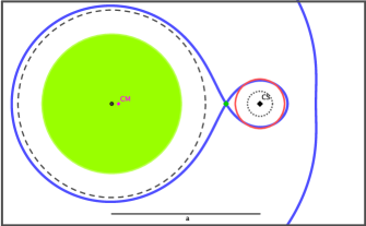
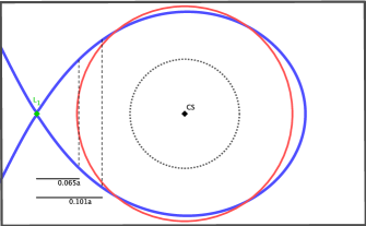
Figure 9: Top view in scale of XB 1916-053 for a mass ratio $q=0.048$. The left and right panel shows the whole binary system and a zoom of it close to the inner Lagrangian point, respectively. The blue curve indicates the Roche lobes of the two stars. The dashed and red circle represent the NS Roche-lobe radius and CS Roche-lobe radius. The magenta, black, and green diamond points are the position of the center of mass (CM), the companion star, and the inner Lagrangian point $L_{1}$. The dotted circle is the radius of the companion star, without thermal inflation. The green circle represents the accretion disk truncated at $0.47a$ (see text). The two black dashed segments indicate the distances from $L_{1}$ at which the matter leaves the binary system for a NS mass of 1.4 M_⊙ at a luminosity of $0.41\times 10^{37}$ erg s^-1 and $1.46\times 10^{37}$ erg s^-1 going from the closest to the farthest.

From the study of the dip arrival times we infer an orbital period derivative $\dot{P}=(1.46\pm 0.03)\times 10^{-11}$ s s^-1 and an orbital period $P=3000.662(1)$ s. Studying eq. 21 for $q=0.048$, we explored the pairs of $\beta$ and $d/a$ for which it is possible to obtain the $\dot{P}$ value assuming NS masses of 1.4, 1.6, and 1.8 M_⊙.

To explain a $\dot{P}$ value of $(1.46\pm 0.03)\times 10^{-11}$ s s^-1, a non-conservative mass transfer is required; we obtain that the parameter $\beta$ has to be smaller than 0.35 for each value of the NS mass studied. We find that the closer the ejection point is to the Lagrangian point, the smaller the fraction of accreted matter is. The possible pairs of $\beta$ and $d/a$ are indicated with the red curve in Fig. 8.

A further constraint on the ejection point and on the fraction of matter accreting onto the NS is given by the luminosity determined in eq. 22. The distance of the source can be estimated using the flux during the type I X-ray bursts observed using Rossi-XTE data, as done by Galloway et al. (2008). Using eq. 10 in Iaria et al. (2015), given that the flux measured during the bursts showing photospheric radius expansion (PRE) is $(2.9\pm 0.4)\times 10^{-8}$ erg s^-1 cm^-2 and that the NS photospheric radius is $r_{PRE}=1.1$ in units of 10 km for XB 1916-053, we find that the distance $D$ to the source is $8.9\pm 0.6$ kpc, $9.3\pm 0.6$ kpc, and $9.6\pm 0.7$ kpc for a NS mass of 1.4, 1.6, and 1.8 M_⊙, respectively. Adopting the 0.1-100 keV unabsorbed flux obtained from spectra A, B, C, and D, we infer that the luminosity varies between $0.41\times 10^{37}$ and $1.46\times 10^{37}$ erg s^-1 for a NS mass of 1.4 M_⊙, between $0.45\times 10^{37}$ and $1.6\times 10^{37}$ erg s^-1 for a NS mass of 1.6 M_⊙, and between $0.48\times 10^{37}$ and $1.7\times 10^{37}$ erg s^-1 for a NS mass of 1.8 M_⊙ by taking into account the error associated with the distance and considering a 10% relative error for the flux. A similar ranges of luminosities were also observed by Boirin et al. (2000), which confirmed that the source belongs to the Atoll class. The 0.1-100 keV unabsorbed luminosities with the corresponding uncertainties are shown in Table 9 for spectra A, B, C, and D.

We plotted the boundary values of luminosity for $q=0.048$ in Fig. 8; since the luminosity depends on $\beta$ but not on the quantity $\alpha=(d/a)^{2}$ (see eq. 22), it is represented with horizontal lines. The observed luminosities constrain $\beta$ to be lower than 15%, independently of the assumed NS mass. The variation in observed luminosity can be explained with a change of the ejection point from which the matter leaves the binary system. At low luminosity the matter leaves the system close to the inner Lagrangian point, and the fraction of mass accretion rate is only 3%, while at higher luminosity the matter leaves the system from a larger distance and $\beta=0.11$. We show a sketch of the top-view geometry (in scale) of XB 1916-053 assuming $q=0.048$ and a NS mass of 1.4 M_⊙ in Fig. 9. The left panel shows the whole binary system, while the right panel shows the companion star and the region close the inner Lagrangian point. The two black dashed segments indicate the boundaries of the ejection region measured from $L_{1}$, the segment distant 0.065$a$ from $L_{1}$. The lower boundary corresponds to a luminosity of $0.41\times 10^{37}$ erg s^-1, while the upper boundary (0.101$a$) corresponds to a luminosity of $1.46\times 10^{37}$ erg s^-1. Similar results are obtained assuming a NS mass of 1.6 and 1.8 M_⊙. Hence, we have shown that abandoning the stringent hypothesis that the matter could leave the system only from the inner Lagrangian point, as supposed by Iaria et al. (2015), a NS mass of 1.4 M_⊙ also describes the observed scenario well.

We note that this scenario assumes that the observed luminosity $L_{\rm obs}$ is that emitted from the source $L_{\rm real}$; however, XB 1916-053 is a dipping source, and so we expect an inclination angle larger than $60^{\circ}$. Since we do not observe eclipses, we can estimate the upper limit on the inclination angle $i$ from the relation $i=90^{\circ}-\arctan(R_{L_{2}}/a)$, where $R_{L_{2}}$ is the Roche lobe radius of the CS, finding that $i<80^{\circ}$. If the emission is not spherical from the innermost region of the system then $L_{\rm obs}=L_{\rm real}\cos{i}$ and we should take into account this amplification factor. By assuming the arbitrary value of $i=70^{\circ}$, the real luminosity varies between $1.2\times 10^{37}$ erg s^-1 and $4.3\times 10^{37}$ erg s^-1. These two values of luminosity combined with the necessity to reproduce an orbital period derivative of $1.46\times 10^{-11}$ s s^-1 gives a value of $\beta$ between 0.08 and 0.34. In this scenario the matter leaves the system at a distance from $L_{1}$ close the CS position.

We note that the mass transfer rate is close to the Eddington limit in this evolutive stage of the source. However, the secular evolution predicts that this system should have a mass transfer rate that is two orders of magnitude lower (see, e.g., Heinke et al. 2013) for a conservative mass transfer scenario.

Table 8: Parameters of XB 1916-053

Parameter
Mass ratio $q$	0.048
Orbital period $P$ (s)	3000.66
Orb. period derivative $\dot{P}$ (s s-1)	$(1.46\pm 0.03)\times 10^{-11}$
Orbital separation $a$a (cm)	$3.54\times 10^{10}$
Roche lobe radius of the CS, $R_{L_{2}}$	$0.156a$
Roche lobe radius of the NS, $R_{L_{1}}$	$0.594a$
Outer radius of the accretion disc, $r$	$0.47a$
Distance of the CM from the NS	$0.046a$
Distance of $L_{1}$ from the NS, $b_{1}$	$0.772a$
Inclination angle $i$	$60^{\circ}<i<80^{\circ}$
Bloating thermal factor $b_{f}$ of the CSa	1.92
Observed luminositya ($10^{37}$ erg s-1)	0.41-1.46
$\beta$b	0.03-0.11
Boundaries of the ejection regionc	0.065$a$-0.101$a$

• Assuming a NS mass of 1.4 M_⊙.

• Fraction of the mass transferred from the CS that accretes onto the NS.

• The boundaries are measured from the inner Lagrangian point $L_{1}$.

Finally, Lasota et al. (2008) discussed the stability of the helium accretion disk in ultracompact X-ray binary systems. From their estimations, the authors suggested that XB 1916-053 should be transient; however, the source is observed as persistent. The authors showed three possible explanations of that incongruity: i) the adopted mass accretion rates (bolometric luminosities) could be underestimated, ii) the outer disk radius is overestimated, iii) the CS is not a pure-helium star, but still contains some hydrogen. From our analysis all the caveats highlighted by the authors are verified. Lasota et al. (2008) assumed a mass accretion rate of $7.6\times 10^{-10}$ M_⊙ yr^-1, while we find from the estimated bolometric fluxes that the mass accretion rate is between $3\times 10^{-10}$ and $1.2\times 10^{-9}$ M_⊙ yr^-1 for a NS mass of 1.4 M_⊙ and NS radius of 10 km. We show that the outer radius of the accretion disk is not truncated at $r_{T}=R_{T}/a=0.6/(1+q),$ which corresponds to $R_{T}=0.57\;a$ for $q=0.048$; it is smaller because of the 3:1 resonance, and we find $r=0.47\;a$. Finally, the fraction of hydrogen is close to 0.2 for a NS mass of 1.4 M_⊙, and increases for higher values of NS mass. We summarized the main parameters of the components of XB 1916-053 in Table 8.

In the following we arbitrarily assume a NS mass of 1.4 M_⊙. Using the mass ratio $q=0.048$, the CS mass is 0.07 M_⊙, the bloating thermal factor of the CS is $b_{f}=1.92$, and the fraction of hydrogen of the CS is close to 20%. We find that the orbital separation of the binary system is $a\simeq 3.54\times 10^{10}$ cm, while the outer radius of the accretion disk is $r_{\rm disk}=1.7\times 10^{10}$ cm.

Iaria et al. (2015) suggest that the sinusoidal modulation obtained from the LQS ephemeris could due to be the presence of a third body gravitationally bound to the X-ray binary system. Assuming the existence of a third body of mass $M_{3}$, the binary system orbits around the new CM of the triple system. The distance of the binary system from the new CM is given by $a_{x}=a_{\rm{bin}}\sin i=A\;c$, where $i$ is the inclination of the binary plane to the plane of the sky, $A$ is the amplitude of the sinusoidal function obtained from the ephemeris shown in Eq. 1, and $c$ is the speed of the light. We obtain $a_{x}=(3.9\pm 0.4)\times 10^{12}$ cm. To infer the mass of the third body we can write its mass function as

$$\frac{M_{3}\sin i}{(M_{3}+M_{\rm{bin}})^{2/3}}=\left(\frac{4\pi^{2}}{G}\right)^{1/3}\frac{a_{x}}{P_{\rm{mod}}^{2/3}},$$

where $M_{\rm{bin}}$ is the mass of the binary system. Assuming arbitrarily $i=70^{\circ}$, we found M${}_{3}\simeq 45$ M_J under the hypothesis that the orbit of the third body is coplanar to the binary system.

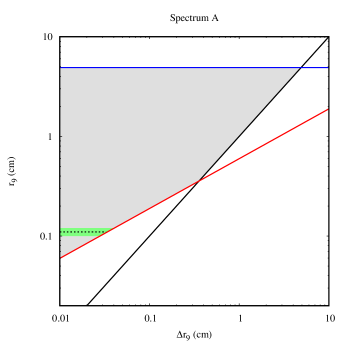
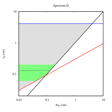
Figure 10: Distance $r$ of the absorber, in units of $10^{9}$ cm, from the NS with respect to its thickness $\Delta r$ (in units of $10^{9}$ cm). The gray area indicates the possible pairs of $r$ and $\Delta r$. The horizontal dashed line indicates the best-fit value of $r$ obtained assuming that the observed redshift is due to gravitational redshift for a NS mass of 1.4 M_⊙; the green area takes into account the associated errors. The black, red, and blue lines are the constraint conditions (see text).

6.4 Ionized absorber

From the spectroscopic analysis we investigated the nature of the ionized absorber around the compact object.

Table 9: Plasma diagnostic of the spectra A, B, C, and D.

	Spectrum A	Spectrum B	Spectrum C	Spectrum D
N${}_{{Ne\textsc{x}}}$a	$0.39\pm 0.09$	$0.37\pm 0.11$	$0.31\pm 0.11$	–
N${}_{{Mg\textsc{xii}}}$	$0.28\pm 0.04$	$0.24\pm 0.04$	$0.26\pm 0.04$	$0.24\pm 0.11$
N${}_{{Si\textsc{xiv}}}$	$0.70\pm 0.03$	$0.59\pm 0.04$	$0.72\pm 0.07$	$1.5\pm 0.4$
N${}_{{S\textsc{xvi}}}$	$0.74\pm 0.15$	$0.61\pm 0.15$	$1.0\pm 0.2$	–
N${}_{{Ca\textsc{xx}}}$	$1.0\pm 0.3$	–	$0.8\pm 0.3$	–
N${}_{{Fe\textsc{xxv}}}$	$1.5\pm 0.3$	–	–	–
N${}_{{Fe\textsc{xxvi}}}$	$7.2\pm 1.3$	$9.6\pm 1.1$	$8.5\pm 1.5$	–
Lxb	$1.5\pm 0.2$	$1.0\pm 0.2$	$0.67\pm 0.11$	$0.41\pm 0.06$
[N${}_{{Ne\textsc{x}}}$]/[NNe]c	$0.24\pm 0.08$	$0.31\pm 0.10$	$0.23\pm 0.09$	–
[N${}_{{Mg\textsc{xii}}}$]/[NMg]	$0.37\pm 0.09$	$0.43\pm 0.09$	$0.41\pm 0.10$	$0.7\pm 0.4$
[N${}_{{Si\textsc{xiv}}}$]/[NSi]	$1.1\pm 0.2$	$1.3\pm 0.2$	$1.4\pm 0.3$	$5\pm 3$
[N${}_{{S\textsc{xvi}}}$]/[NS]	$3.0\pm 0.9$	$3.3\pm 0.9$	$4.7\pm 1.2$	–
[N${}_{{Ca\textsc{xx}}}$]/[NCa]	$24\pm 9$	–	$23\pm 10$	–
[N${}_{{Fe\textsc{xxv}}}$]/[NFe]	$2.5\pm 0.9$	–	–	–
[N${}_{{Fe\textsc{xxvi}}}$]/[NFe]	$12\pm 3$	$22\pm 4$	$17\pm 4$	–

• The equivalent column density of the ions shown are in units of 10¹⁷ atoms cm^-2.

• Unabsorbed extrapolated luminosity in the 0.1-100 keV energy range. The luminosity is in units of $10^{37}$ erg s^-1 for a NS mass of 1.4 M_⊙.

• The ratio is in units of $10^{-2}$.

Initially we estimated the equivalent column densities of the ions producing the absorption lines in spectra A, B, C, and D. To do this we used the relation shown by Spitzer (1978)

$$\frac{W_{\lambda}}{\lambda}=\frac{\pi e^{2}}{m_{e}c^{2}}N_{j}\lambda f_{ij}\simeq 8.85\;10^{-13}N_{j}\lambda f_{ij},$$

where $N_{j}$ is the equivalent column density for the relevant species, $f_{ij}$ is the oscillator strength, $W_{\lambda}$ is the equivalent width of the line, $\lambda$ is the wavelength in centimeters, $e$ is the electron charge, $m_{e}$ is the electron mass, and $c$ is the speed of the light. A similar analysis was done for the dipping source XB 1254-690 (Iaria et al. 2007a) and X 1624-690 (Iaria et al. 2007b) and, recently, for XB 1916-053 using Suzaku data (Gambino et al. 2019). To infer the column densities of the ions we assumed $f_{ij}=0.416$ for all the H-like ions and $f_{ij}=0.798$ for the Fe xxv ion (Verner et al. 1996b), and we used the equivalent widths shown in Table 6; the inferred $N_{j}$ values are shown in Table 9. We find that the equivalent ion column density is in the range between $10^{16}$ and $(7.2-8.5)\times 10^{17}$ cm^-2.

We estimated the abundances of each ion with respect to the neutral element $N_{\rm ion}/N_{\rm el}$. To this end, we used the values of the neutral hydrogen equivalent column density of the ionized absorber, N${}_{{\rm H}_{\xi}}$, shown in Table 5 and we adopted the relation $N_{{\rm H}_{\xi}}=N_{{\rm H}_{\xi}}/N_{\rm el}\;N_{\rm el}/N_{\rm ion}\;N_{\rm ion}$, where $N_{{\rm H}_{\xi}}/N_{\rm el}$ is the inverse of a given element with respect to the hydrogen and $N_{\rm ion}$ is the value of the equivalent column density associated with the ions shown in Table 9. To infer the value of $N_{\rm ion}/N_{\rm el}$ we adopted the solar abundance shown by Asplund et al. (2009). The values of $N_{\rm ion}/N_{\rm el}$ for spectra A, B, C, and D are shown in Table 9. We find that the ratio $N_{\rm ion}/N_{\rm el}$ is 0.2%, 0.4%, 1-2%, 3-4%, $(24\pm 10)$%, 2.5%, and 10-20% for Ne x, Mg xii, Si xiv, S xvi, Ca xx, Fe xxv, and Fe xxvi, respectively. In a scenario where the NS mass is 1.4 M_⊙, the fraction of hydrogen of the CS is close to 20%; because $X\simeq 0.7$ for solar abundance, we should roughly multiply the adopted abundances by a factor of three. Consequently, the ion population with respect to a given neutral element should be reduced by a factor of $1/3$.

To estimate the region where the ionized absorber is located, we used the definition of $\xi$ in zxipcf from which we get $r^{2}=L_{x}/(n_{H}\xi)$, where $L_{x}$ is the unabsorbed luminosity in the 0.1-100 keV energy range, $r$ is the distance of the absorber from the central source, $\xi$ is the ionization parameter obtained by our fits, and $n_{H}$ is the hydrogen atom density of the absorber. By combining the last equation with N${}_{{\rm H}_{\xi}}=n_{H}\Delta r$, where $\Delta r$ is the geometrical thickness of the absorber along the line of sight and N${}_{{\rm H}_{\xi}}$ is the equivalent hydrogen column density associated with the absorber, and by imposing $r>\Delta r$, we obtained an upper limit on $r$ that is $r<L_{x}/(N_{{\rm H}_{\xi}}\xi)$. Furthermore, we expect that the optical depth $\tau=\sigma_{T}N_{{\rm H}_{\xi}}$ of the absorber is lower than one, where $\sigma_{T}$ is the Thomson cross section. By rearranging $r^{2}=L_{x}/(n_{H}\xi)$, we obtain $r^{2}=L_{x}\sigma_{T}\Delta r/(\tau\xi),$ and consequently $r>(L_{x}\sigma_{T}\Delta r/\xi)^{1/2}$. By using the best-fit values of N${}_{{\rm H}_{\xi}}$ and $\xi$ shown in Table 5 and the 0.1-100 keV unabsorbed luminosities shown in Table 9 we are able to constrain the region where the ionized absorber is placed.

We show the distance of the absorber from the NS in units of $10^{9}$ cm with respect to the thickness $\Delta r$ in units of $10^{9}$ cm in Fig. 10. The condition $r<L_{x}/(N_{{\rm H}_{\xi}}\xi)$ is represented with a blue line, $r>\Delta r$ is indicated with a black line, and $r>(L_{x}\sigma_{T}\Delta r/\xi)^{1/2}$ with a red line. The gray area gives the pairs of $r$ and $\Delta r$ satisfying the conditions. Since the outer radius of the accretion disk is $1.7\times 10^{10}$ cm and because the maximum value of $r$ is roughly $5\times 10^{9}$ cm, we conclude that the ionized absorber is placed in the innermost region of the system.

After analyzing the same Chandra data, Trueba et al. (2020) suggests that the observed redshift in the absorption lines is probably due to gravitational redshift, and finds the distance of the absorber from the NS is $(2.7\pm 1.7)\times 10^{8}$ cm and $(2.3\pm 1.2)\times 10^{8}$ cm for a NS mass of 1.4 M_⊙; these values refer to spectra B and $\Gamma$ reported by the authors. By adopting the same scenario and using the best-fit values of the observed redshift shown in Table 5 we find that the absorber is placed at $(1.1\pm 0.1)\times 10^{8}$ cm, $(1.3\pm 0.2)\times 10^{8}$ cm, $(1.2\pm 0.2)\times 10^{8}$ cm, and $(1.3\pm 0.7)\times 10^{8}$ cm for spectra A, B, C, and D, respectively. Our estimations are almost a factor of two smaller than the value estimated by Trueba et al. (2020), even if the values are compatible with each other. We show the best-fit value of $r$ and the associated errors with a dashed line and the green area in Fig. 10. We find that the ionized absorber can reach the NS surface only in spectrum D when the source is dimmer; in the other cases the absorber forms a torus around the compact object. From N${}_{{\rm H}_{\xi}}=n_{H}\Delta r$ we can infer the lower limit of $n_{H}$ assuming the maximum possible thickness of the absorber; we obtain $n_{H}>5\times 10^{15}$ cm^-3, $n_{H}>2\times 10^{15}$ cm^-3, $n_{H}>1.5\times 10^{15}$ cm^-3, and $n_{H}>0.4\times 10^{15}$ cm^-3 for spectra A, B, C, and D.

We repeated the same procedure to estimate the distance of the absorber during the dip using the values in Table 7 and knowing that the 0.1-100 keV unabsorbed luminosity is $(0.6\pm 0.1)\times 10^{37}$ erg s^-1. We find a weak constraint for $r$; it is between $2\times 10^{8}$ and $1.7\times 10^{10}$ cm (the outer radius of the disk). Because of the low value of the ionization parameter it is possible that the absorber is placed at the outer radius; however, we cannot exclude inner radii. We note that the circularization radius $r_{\rm circ}=0.0859\;a\;q^{-0.426}$ (valid for $q$ between 0.05 and 1; Hessman & Hopp 1990) is $r_{\rm circ}\simeq 1.1\times 10^{10}$ cm for $q=0.048$, compatible with the obtained distances.

Finally, we explored the nature of the O viii absorption edge observed in the spectra during the persistent emission. Since its optical depth is $0.16$, assuming that $n_{e}\sim n_{i}$, we can write $\tau=N_{H}\sigma_{T}$, where $\sigma_{T}$ is the Thomson cross section. We inferred an equivalent hydrogen column density of $\sim 2.3\times 10^{23}$ cm^-2. This value is compatible with the equivalent hydrogen column associated with the ionized absorber. We conclude that a small fraction of O viii could be present in the absorber.

7 Conclusions

We updated the orbital ephemeris of the compact dipping source XB 1916-053 by analyzing ten new Chandra observations and one Swift/XRT observation. Three new dip arrival times were extracted, allowing us to extend the available baseline from 36 to 40 years. Our analysis definitively excludes several models of ephemeris suggested previously, leaving as a more likely candidate the quadratic orbital ephemeris including a large periodic modulation close to 25 years (LQS ephemeris in this work).

The quadratic term of the orbital ephemeris implies the presence of an orbital period derivative of $1.46(3)\times 10^{-11}$ s s^-1, and allows us to refine the orbital period measurement to 3000.662(1) s. We confirm that such a fast orbital expansion implies that mass transfer should be highly non-conservative. Moreover, we find that for a NS mass of $1.4$ M_⊙ it is possible to obtain a compatible orbital period derivative and luminosity values, releasing the stringent hypothesis that the mass leaves the system at the inner Lagrangian point. For a NS mass of $1.4$ M_⊙ we find that the ejection point is distant from the inner Lagrangian point between $3\times 10^{8}$ and $1.5\times 10^{9}$ cm.

We show that the mass ratio of the system is $q=0.048$. This value is obtained from the observed infrahump period, as already discussed in the literature by Hu et al. (2008), and from the observed superhump period, which introduces the pressure term due to a spiral wave to explain the apsidal precession period of the accretion disk. Our study allows us to explain the infrahump and superhump periods (Chou et al. 2001), assuming that the accretion disk has a prograde apsidal precession of 3.9 days and a retrograde nodal precession of 4.86 days. The outer radius of the accretion disk is truncated where the 3:1 resonance occurs (i.e., $1.7\times 10^{10}$ cm for a NS mass of 1.4 M_⊙).

Assuming a NS mass of 1.4 M_⊙, we obtain that the CS mass is 0.07 M_⊙. The thermal bloating of the CS is 1.92 and its percentage of content hydrogen is 20%.

We explain the periodic modulation observed in the orbital ephemeris as the presence of a third body orbiting around the binary system. Assuming a co-planar orbit with respect to the binary system, an inclination angle of $70^{\circ}$, and a hierarchical triple system, we find that the mass of the third body is $M_{3}\simeq 45$ Jovian masses.

To perform our spectroscopic analysis we also included an old Chandra observation, previously analyzed by Iaria et al. (2006). We observed a large variation in the count rate for the different observations. Using a Comptonized component for the continuum we estimated that the 0.1-100 keV unabsorbed luminosity varies from $0.41\times 10^{37}$ erg ^-1 to $1.46\times 10^{37}$ erg ^-1 during the persistent emission.

The spectra show the presence of prominent absorption lines associated with Ne x, Mg xii, Si xiv, S xvi, and Fe xxvi. To fit these lines we included in the model the component zxipcf that assumes the presence of an ionized absorber between the central object and the observer along the line of sight. We find that the equivalent hydrogen column density associated with the ionized absorber ranges from $9\times 10^{22}$ cm^-2 to $2\times 10^{23}$ cm^-2, going from the dimmest to the brightest spectrum. The ionization parameter is close to log${(\xi)}=4.3$. From our diagnostic, under the assumption that the observed redshift of the line produced in the absorber is due to gravitational redshift, as recently discussed by Trueba et al. (2020), we find that the absorber has a hydrogen atom density $n_{H}$ higher than $10^{15}$ cm^-3 and it is located far from the central source at $1\times 10^{8}$ cm for a NS mass of 1.4 M_⊙.

We extracted the dip spectrum finding that the equivalent hydrogen column density associated with the ionized absorber is $6\times 10^{23}$ cm^-2 and the ionization parameter is close to log${(\xi)}=2.8$. Finally, we find that during the dip the ionized absorber is placed at a greater distance, which could be compatible with the edge of the accretion disk ($1.7\times 10^{10}$ cm) even if we cannot exclude that it is placed at the circularization radius ($1.0\times 10^{10}$ cm).

References

- Asplund et al. (2009) Asplund, M., Grevesse, N., Sauval, A. J., & Scott, P. 2009, ARA&A, 47, 481
- Boirin et al. (2000) Boirin, L., Barret, D., Olive, J. F., Bloser, P. F., & Grindlay, J. E. 2000, A&A, 361, 121
- Boirin et al. (2004) Boirin, L., Parmar, A. N., Barret, D., Paltani, S., & Grindlay, J. E. 2004, A&A, 418, 1061
- Brouwer & Clemence (1961) Brouwer, D. & Clemence, G. M. 1961, Methods of celestial mechanics
- Burrows et al. (2005) Burrows, D. N., Hill, J. E., Nousek, J. A., et al. 2005, Space Sci. Rev., 120, 165
- Callanan et al. (1995) Callanan, P. J., Grindlay, J. E., & Cool, A. M. 1995, PASJ, 47, 153
- Chou et al. (2001) Chou, Y., Grindlay, J. E., & Bloser, P. F. 2001, ApJ, 549, 1135
- Cumming (2003) Cumming, A. 2003, ApJ, 595, 1077
- Eggleton (1983) Eggleton, P. P. 1983, ApJ, 268, 368
- Frank et al. (2002) Frank, J., King, A., & Raine, D. J. 2002, Accretion Power in Astrophysics: Third Edition
- Galloway et al. (2008) Galloway, D. K., Muno, M. P., Hartman, J. M., Psaltis, D., & Chakrabarty, D. 2008, ApJS, 179, 360
- Gambino et al. (2019) Gambino, A. F., Iaria, R., Di Salvo, T., et al. 2019, A&A, 625, A92
- Gehrels et al. (2004) Gehrels, N., Chincarini, G., Giommi, P., et al. 2004, ApJ, 611, 1005
- Goodchild & Ogilvie (2006) Goodchild, S. & Ogilvie, G. 2006, MNRAS, 368, 1123
- Grindlay et al. (1988) Grindlay, J. E., Bailyn, C. D., Cohn, H., et al. 1988, ApJ, 334, L25
- Heinke et al. (2013) Heinke, C. O., Ivanova, N., Engel, M. C., et al. 2013, ApJ, 768, 184
- Hellier (2001) Hellier, C. 2001, Cataclysmic Variable Stars
- Hessman & Hopp (1990) Hessman, F. V. & Hopp, U. 1990, A&A, 228, 387
- Hirose & Osaki (1990) Hirose, M. & Osaki, Y. 1990, PASJ, 42, 135
- Hu et al. (2008) Hu, C.-P., Chou, Y., & Chung, Y.-Y. 2008, ApJ, 680, 1405
- Iaria et al. (2015) Iaria, R., Di Salvo, T., Gambino, A. F., et al. 2015, A&A, 582, A32
- Iaria et al. (2007a) Iaria, R., di Salvo, T., Lavagetto, G., D’Aí, A., & Robba, N. R. 2007a, A&A, 464, 291
- Iaria et al. (2006) Iaria, R., Di Salvo, T., Lavagetto, G., Robba, N. R., & Burderi, L. 2006, ApJ, 647, 1341
- Iaria et al. (2007b) Iaria, R., Lavagetto, G., D’Aí, A., di Salvo, T., & Robba, N. R. 2007b, A&A, 463, 289
- Iaria et al. (2019) Iaria, R., Mazzola, S. M., Bassi, T., et al. 2019, A&A, 630, A138
- Juett & Chakrabarty (2006) Juett, A. M. & Chakrabarty, D. 2006, ApJ, 646, 493
- Larwood et al. (1996) Larwood, J. D., Nelson, R. P., Papaloizou, J. C. B., & Terquem, C. 1996, MNRAS, 282, 597
- Lasota et al. (2008) Lasota, J. P., Dubus, G., & Kruk, K. 2008, A&A, 486, 523
- Lubow (1991a) Lubow, S. H. 1991a, ApJ, 381, 259
- Lubow (1991b) Lubow, S. H. 1991b, ApJ, 381, 268
- Lubow (1992) Lubow, S. H. 1992, ApJ, 401, 317
- Miller et al. (2007) Miller, L., Turner, T. J., Reeves, J. N., et al. 2007, A&A, 463, 131
- Montgomery (2001) Montgomery, M. M. 2001, MNRAS, 325, 761
- Montgomery (2009) Montgomery, M. M. 2009, ApJ, 705, 603
- Nelemans et al. (2006) Nelemans, G., Jonker, P. G., & Steeghs, D. 2006, MNRAS, 370, 255
- Paczynski (1977) Paczynski, B. 1977, ApJ, 216, 822
- Paczynski & Sienkiewicz (1981) Paczynski, B. & Sienkiewicz, R. 1981, ApJ, 248, L27
- Papaloizou & Terquem (1995) Papaloizou, J. C. B. & Terquem, C. 1995, MNRAS, 274, 987
- Patterson et al. (2005) Patterson, J., Kemp, J., Harvey, D. A., et al. 2005, PASP, 117, 1204
- Pearson (2006) Pearson, K. J. 2006, MNRAS, 371, 235
- Plavec & Kratochvil (1964) Plavec, M. & Kratochvil, P. 1964, Bulletin of the Astronomical Institutes of Czechoslovakia, 15, 165
- Ponti et al. (2015) Ponti, G., Bianchi, S., Muñoz-Darias, T., et al. 2015, MNRAS, 446, 1536
- Rappaport et al. (1987) Rappaport, S., Nelson, L. A., Ma, C. P., & Joss, P. C. 1987, ApJ, 322, 842
- Reeves et al. (2008) Reeves, J., Done, C., Pounds, K., et al. 2008, MNRAS, 385, L108
- Retter et al. (2002) Retter, A., Chou, Y., Bedding, T. R., & Naylor, T. 2002, MNRAS, 330, L37
- Smale et al. (1989) Smale, A. P., Mason, K. O., Williams, O. R., & Watson, M. G. 1989, PASJ, 41, 607
- Spitzer (1978) Spitzer, L. 1978, Physical processes in the interstellar medium
- Swank et al. (1984) Swank, J. H., Taam, R. E., & White, N. E. 1984, ApJ, 277, 274
- Trueba et al. (2020) Trueba, N., Miller, J. M., Fabian, A. C., et al. 2020, ApJ, 899, L16
- Verner et al. (1996a) Verner, D. A., Ferland, G. J., Korista, K. T., & Yakovlev, D. G. 1996a, ApJ, 465, 487
- Verner et al. (1996b) Verner, D. A., Verner, E. M., & Ferland, G. J. 1996b, Atomic Data and Nuclear Data Tables, 64, 1
- Walter et al. (1982) Walter, F. M., Mason, K. O., Clarke, J. T., et al. 1982, ApJ, 253, L67
- White (1989) White, N. E. 1989, A&A Rev., 1, 85
- White & Swank (1982) White, N. E. & Swank, J. H. 1982, ApJ, 253, L61
- Whitehurst (1988) Whitehurst, R. 1988, MNRAS, 232, 35
- Wilms et al. (2000) Wilms, J., Allen, A., & McCray, R. 2000, ApJ, 542, 914
- Zdziarski et al. (1996) Zdziarski, A. A., Johnson, W. N., & Magdziarz, P. 1996, MNRAS, 283, 193