Electric probe for the toric code phase in Kitaev materials
through the hyperfine interaction

Abstract

The Kitaev model is a remarkable spin model with gapped and gapless spin liquid phases, which are potentially realized in iridates and $\alpha$-RuCl₃. In the recent experiment of $\alpha$-RuCl₃, the signature of a nematic transition to the gapped toric code phase, which breaks the $C_{3}$ symmetry of the system, has been observed through the angle dependence of the heat capacity. We here propose a mechanism by which the nematic transition can be detected electrically. This is seemingly impossible because $J_{\textrm{eff}}=1/2$ spins do not have an electric quadrupole moment (EQM). However, in the second-order perturbation the virtual state with a nonzero EQM appears, which makes the nematic order parameter detectable by nuclear magnetic resonance and Mössbauer spectroscopy. The purely magnetic origin of EQM is different from conventional electronic nematic phases, allowing the direct detection of the realization of Kitaev’s toric error-correction code.

Introduction.— The Kitaev model Kitaev (2006) is a notable spin model for quantum spin liquids (QSLs) with gapped and gapless ground states. After pioneering work by Jackeli and Khaliullin Jackeli and Khaliullin (2009), potential experimental realizations were reported in iridates Singh and Gegenwart (2010); Singh et al. (2012) and $\alpha$-RuCl₃ Plumb et al. (2014). Indeed, those materials have $d^{5}$ metal ions in the octahedral ligand field forming the honeycomb lattice, which results in unusual anisotropic interactions proposed by Kitaev Kitaev (2006). This Jackeli-Khaliullin mechanism is intrinsic to the $J_{\textrm{eff}}=1/2$ magnetic moment with a strong spin-orbit coupling (SOC), and makes the $d^{5}$ materials family, sometimes called Kitaev materials, a fascinating platform for the physics of Majorana fermions. Especially, after the discovery of a field-revealed QSL phase in $\alpha$-RuCl₃ Kasahara et al. (2018a, b), various experimental techniques were used to characterize this exotic phase under a magnetic field Banerjee et al. (2018); Janša et al. (2018); Lebert et al. (2020). However, the realization of Kitaev’s gapped $A$ phase, which is nothing but a toric code phase Kitaev (2003), was only discussed in a complex structure in metal-organic frameworks Yamada et al. (2017a).

Kitaev’s $A$ phase is the ground state of the Kitaev model in the anisotropic limit. This is a gapped $Z_{2}$ spin liquid phase and is mapped to the toric code model in the fourth order perturbation. The toric code is a topological error correction code which is useful in fault-tolerant quantum computing. We here discuss another route towards the realization of this phase. This toric code phase is potentially realized by a spontaneous breaking of the $C_{3}$ symmetry of the isotropic Kitaev model. If the order parameter reaches a critical value, the system transforms from $B$ phase to $A$ phase. This order parameter consists of quadrupole operators, rather than usual magnetic dipoles, and in this sense we can regard it as a nematic transition.

On the analogy of liquid crystals, a nematic phase is discussed in various fields of condensed matter physics, ranging from spin nematic phases in frustrated magnets Penc and Läuchli (2011) to electronic nematic phases in quantum Hall systems Lilly et al. (1999), ruthanates Borzi et al. (2007), unconventional superconductors de la Cruz et al. (2008), etc. Inspired by the previous numerical studies Gordon et al. (2019); Lee et al. (2020), we seek for a possibility of the nematic transition in Kitaev materials. In $J_{\textrm{eff}}=1/2$ Kitaev materials, it should be called spin-orbital nematic Li et al. (2020) with properties of both spin nematic and electronic nematic.

Recently, O. Tanaka et al. Tanaka et al. indeed observed such a spin-orbital nematic transition from a gapped chiral spin liquid phase to a different gapped phase characterized by the broken threefold rotation ($C_{3}$) symmetry, based on the measurements of the angle dependence of heat capacity under a strong magnetic field. It has been proposed that this symmetry-broken phase could be the toric code phase Takahashi et al. (2021), as the half-quantized thermal Hall effect disappears at the transition point Kasahara et al. (2018b). However, the property of this nematic transition is still obscure, and we need a more sensitive local probe for this unusual phase transition.

Therefore, we propose an electric quadrupole moment (EQM) as a direct probe for the topological nematic transition Takahashi et al. (2021) of the $J_{\textrm{eff}}=1/2$ magnetic moments. This statement is very counterintuitive as the $J_{\textrm{eff}}=1/2$ pseudospin does not have an EQM in the cubic environment, differently from the $J_{\textrm{eff}}=3/2$ case Yamada et al. (2018), where the quadrupole moment is directly measurable. Interestingly, however, holes with a $J_{\textrm{eff}}=1/2$ pseudospin can hop to the nearest-neighbor (NN) sites, and an virtual state with two holes can possess an EQM. This is because via the superexchange pathway involving the Cl $p$-orbitals the $J_{\textrm{eff}}=1/2$ state can be transformed into a state with a nonzero quadrupole moment. This enables us to electrically detect the nematic order parameter, which is originally written in terms of spin operators. We also discuss that, although the Chern number is not measurable, its change can be inferred from the careful analysis of the derivative of the in-plane anisotropy parameter $\eta$.

In a real experimental setup, the most sensitive way to measure the EQM is through the hyperfine interaction because the nuclear with a spin $I\geq 1$ can feel the electric field gradient (EFG), or the EQM. Especially, nuclear magnetic resonance (NMR) and Mössbauer spectroscopy (MS) use a nuclear spin of Ru as a direct probe, and they are highly sensitive to the symmetry of the local environment. If the $C_{3}$ symmetry of Ru forming the honeycomb lattice is broken, it can potentially be detected by ^99/101Ru-NMR Majumder et al. (2015), or ⁹⁹Ru-MS Kobayashi et al. (1992). In NMR and MS, the in-plane anisotropy is characterized by a single dimensionless parameter $\eta$ Toyoda et al. (2018a, b); Kitagawa et al. (2018). If the EFG or EQM tensor has an anisotropy around the [111] axis, $\eta$ gets nonzero and the signal splits or shifts, which could detect the existence of a nematic order.

In this Letter, we will prove that the in-plane anisotropy $\eta$ is directly connected to the nematic order parameter in terms of Majorana fermions, which potentially detects the transition to the toric code phase.

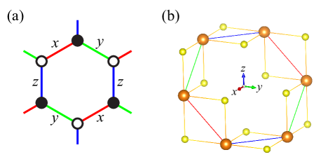
Figure 1: (a) Honeycomb lattice where the Kitaev model is defined. Red, green, and blue bonds represent bonds in the $x$-, $y$-, and $z$-directions, respectively. (b) Idealized geometry of $\alpha$-RuCl₃. Orange and yellow spheres represent Ru and Cl ions, respectively. Bonds in the $\gamma$-direction are defined to be perpendicular to the $\gamma$-axis of the cubic lattice. The figure is generated by VESTA Momma and Izumi (2011).

Quadrupole moment.— An electronic EQM is defined for $d$-orbitals by

$$q^{\alpha\beta}=\frac{3}{2}(L^{\alpha}L^{\beta}+L^{\beta}L^{\alpha})-\bm{L}^{2}\delta^{\alpha\beta},$$ (1)

where $\bm{L}$ are $L=2$ orbital angular momentum operators of Ru $d$-orbitals and $\alpha=x$, $y$, or $z$, and $\beta=x$, $y$, or $z$. This rank-2 traceless symmetric tensor directly couples to the nuclear EQM of Ru, and the anisotropy of $q^{\alpha\beta}$ is easily measurable. If the EFG from the surrounding ions is negligible as is the case for ⁹⁹Ru-MS Kobayashi et al. (1992), we can identify the effective EFG $V_{\textrm{eff}}^{\alpha\beta}$ to be proportional to $q^{\alpha\beta}$. Therefore, we will not distinguish between EFG and EQM of Ru from now on.

The definition of $\eta$ in terms of $q^{\alpha\beta}$ is as follows. Since this tensor is symmetric, it can be diagonalized by orthogonal transformation. Here we denote the principal axis as $abc$, where we define the order of $abc$ such that $|q^{cc}|\geq|q^{bb}|\geq|q^{aa}|$. In this case, $\eta$ is defined as $\eta=(q^{aa}-q^{bb})/q^{cc}$. If $\eta=0$, it is apparent that EQM is invariant under the rotation around the $c$-axis, and thus it potentially detects the breaking of the $C_{3}$ symmetry of $\alpha$-RuCl₃. However, the connection between $\eta$ and the nematic order parameter is not evident in this form. Differently from the “electronic” nematic order, where $\eta$ detects the distortion of surrounding ligands, the spin nematic order is subtle without a detectable structural transition.

Since the nematic transition of $\alpha$-RuCl₃ may be purely magnetic as around the transition point $H\sim 10$ T no structural transition has been observed Tanaka et al. , we have to think of a mechanism where a pure spin operator is transformed into an electric quadrupole. Especially, in the case where the position of Cl ligands is not distorted, we have to consider a purely electronic origin for this mechanism, which involves a microscopic structure of Ru $d$-orbitals. From now on we set $\hbar=1$.

As is well-known, the $J_{\textrm{eff}}=1/2$ pseudospin cannot possess an EQM in the cubic environment, thus we have to perturb the $J_{\textrm{eff}}=1/2$ wavefunction in some way to get a nonzero expectation value of EQM. One simple way is by the ligand field effect of the lattice distortion, but it only produces a static contribution. A more exotic answer is to perturb the $J_{\textrm{eff}}=1/2$ wavefunction via the superexchange mechanism. Especially, in the case of the low-spin $d^{5}$ configuration, it is well-known as the Jackeli-Khaliullin mechanism that the $J_{\textrm{eff}}=1/2$ state is transformed into $J_{\textrm{eff}}=3/2$ state with a nonzero quadrupole moment, which produces the following Kitaev Hamiltonian for $J_{\textrm{eff}}=1/2$ pseudospins:

$$\mathcal{H}_{\textrm{Kitaev}}=-K\sum_{\langle ij\rangle\in\gamma}S_{i}^{\gamma}S_{j}^{\gamma},$$ (2)

where $\bm{S}_{i}$ is a pseudospin on the $i$th site of $\alpha$-RuCl₃, $K>0$ is a Kitaev interaction, and $\langle ij\rangle\in\gamma$ means an NN bond $\langle ij\rangle$ in the $\gamma$-direction with $\gamma=x$, $y$, and $z$. The bond direction is defined as illustrated in Fig. 1(a). Assuming the 0-flux ground state, the Hamiltonian can be recast into the tight-binding model of Majorana fermions.

$$\mathcal{H}_{\textrm{Majorana}}=\frac{K}{4}\sum_{\langle ij\rangle}ic_{i}c_{j},$$ (3)

where $c_{i}$ is an itinerant Majorana fermion on the $i$th site. We note that in this Letter we do not antisymmetrize Majorana fermion operators.

Similarly to the Jackeli-Khaliullin mechanism, we can compute an effective quadrupole moment produced by the virtual state, and it can potentially have a form of $S_{i}^{\gamma}S_{j}^{\gamma}$. This is how the pure spin operator $S_{i}^{\gamma}S_{j}^{\gamma}$ can be transformed into an electric quadrupole $q^{\gamma\gamma}$ in the second-order perturbation.

Second-order perturbation.— Following Jackeli and Khaliullin Jackeli and Khaliullin (2009), we will do the perturbation inside the $t_{2g}$-orbitals assuming a large octahedral ligand field. The discussion also follows Refs. Bolens et al. (2018); Bolens (2018); Pereira and Egger (2020). Especially, the idea is related to the one discussed in Ref. Bulaevskii et al. (2008). We first note that $t_{2g}$-orbitals ($d_{yz}$, $d_{xz}$, and $d_{xy}$) possess an effective angular momentum operator $\bm{l}_{\textrm{eff}}$ with $l_{\textrm{eff}}=1$. This effective moment has a relation $\bm{L}=-\bm{l}_{\textrm{eff}}$ inside the $t_{2g}$-manifold, but we cannot simply use this relation in the calculation of $q^{\alpha\beta}$. The computation of $q^{\alpha\beta}$ involves intermediate $e_{g}$-orbitals, which brings about a nonzero correction. Details are included in Supplemental Material (SM) SM .

We take the following basis set to write down the Hamiltonian:

$$\bm{d}_{i}^{\dagger}=\left(d_{i,yz,\uparrow}^{\dagger},d_{i,yz,\downarrow}^{\dagger},d_{i,xz,\uparrow}^{\dagger},d_{i,xz,\downarrow}^{\dagger},d_{i,xy,\uparrow}^{\dagger},d_{i,xy,\downarrow}^{\dagger}\right),$$ (4)

where $d_{i,\alpha,\sigma}^{\dagger}$ denotes a hole creation operator for a $d_{\alpha}$-orbital with a spin $\sigma=\uparrow$, $\downarrow$ with $\alpha=yz$, $xz$, and $xy$. We sometimes identify $yz$, $xz$, and $xy$ with $x$, $y$, and $z$, respectively.

The Hamiltonian $\mathcal{H}$ consists of the following terms:

$$\mathcal{H}=\mathcal{H}_{\textrm{hop}}+\mathcal{H}_{\textrm{SOC}}+\mathcal{H}_{\textrm{LF}}+\mathcal{H}_{\textrm{Hubbard}},$$ (5)

which is the sum of the kinetic hopping term, the SOC, the ligand field splitting, and the Hubbard term. The kinetic hopping term can be written generically as follows:

$$\mathcal{H}_{\textrm{hop}}=-\sum_{\langle ij\rangle\in\gamma}\left[\bm{d}_{i}^{\dagger}(T^{\gamma}\otimes\openone_{2})\bm{d}_{j}+\textrm{H.c.}\right],$$ (6)

where $\openone_{n}$ is the $n\times n$ identity matrix, and $T^{\gamma}$ with $\gamma=x$, $y$, and $z$ are

$$T^{x} =\begin{pmatrix}0&0&0\\ 0&0&t_{2}\\ 0&t_{2}&0\end{pmatrix},\quad T^{y}=\begin{pmatrix}0&0&t_{2}\\ 0&0&0\\ t_{2}&0&0\end{pmatrix},$$

$$T^{z} =\begin{pmatrix}0&t_{2}&0\\ t_{2}&0&0\\ 0&0&0\end{pmatrix},$$ (7)

where $t_{2}$ is the main contribution coming from the pathway via Cl $p$-orbitals. Of course, we can consider a more generic form including $t_{i}$ ($i=1,\dots,4$) Bolens et al. (2018); Bolens (2018).

The SOC Hamiltonian is $\mathcal{H}_{\textrm{SOC}}=(\lambda/2)\sum_{i,\alpha}\bm{d}_{i}^{\dagger}(l^{\alpha}\otimes\sigma^{\alpha})\bm{d}_{i}$, where $\lambda>0$, $(l^{\alpha})_{\beta\gamma}=-i\epsilon_{\alpha\beta\gamma}$, and $\sigma^{\alpha}$ are Pauli matrices with $\alpha=x$, $y$, and $z$. $\mathcal{H}_{\textrm{LF}}=\Delta\sum_{i}\bm{d}_{i}^{\dagger}\left[(\bm{l}\cdot\hat{\bm{n}})^{2}\otimes\openone_{2}\right]\bm{d}_{i}$ with $\hat{\bm{n}}=(1,1,1)/\sqrt{3}$, assuming the preserved $C_{3}$ symmetry of the lattice.

$\mathcal{H}_{\textrm{Hubbard}}$ is a multiorbital Hubbard interaction term. We here ignore the Hund coupling $J_{H}$ for simplicity as $J_{H}$ is much smaller than the Hubbard interaction $U$. $\mathcal{H}_{\textrm{Hubbard}}=(U/2)\sum_{i}{n_{i}(n_{i}-1)}$, where $n_{i}=\bm{d}_{i}^{\dagger}\cdot\bm{d}_{i}$ is a number operator for each site.

Let us begin with the case without a ligand field splitting by setting $\Delta=0$. In the atomic limit without a kinetic term, the system has exactly one hole per site. The states for a single hole are split into $J_{\textrm{eff}}=3/2$ and $J_{\textrm{eff}}=1/2$, and the atomic ground state consists of degenerate $J_{\textrm{eff}}=1/2$ pseudospins as $\lambda>0$, which is denoted by $\bm{S}_{i}$. The effective operator form of $q^{\alpha\beta}$ in terms of pseudospins $\bm{S}_{i}$ can be derived from the second-order perturbation in the kinetic term. This is achieved by perturbing a magnetic state $\ket{\phi_{m}}$ into $\ket{\psi_{m}}$ up to the first order and by computing

$$\left[q_{\textrm{eff}}^{\alpha\beta}\right]_{mn}=\braket{\psi_{m}}{q^{\alpha\beta}}{\psi_{n}}.$$ (8)

$\ket{\psi_{m}}$ is

$$\ket{\psi_{m}}=\alpha\ket{\phi_{m}}+\frac{1-P}{E_{0}-\mathcal{H}_{0}}\mathcal{H}_{\textrm{hop}}\ket{\phi_{m}},$$ (9)

where $\alpha\sim 1$ is a renormalization constant, $P$ is a projection operator onto unperturbed states, and $\mathcal{H}_{0}$ is an unperturbed Hamiltonian with an energy $E_{0}$ for $\ket{\phi_{m}}$. Since the original $J_{\textrm{eff}}=1/2$ state $\ket{\phi_{m}}$ does not have an EQM, the effective operator can finally be written

$$q_{\textrm{eff}}^{\alpha\beta}=P\mathcal{H}_{\textrm{hop}}\frac{1-P}{E_{0}-\mathcal{H}_{0}}q^{\alpha\beta}\frac{1-P}{E_{0}-\mathcal{H}_{0}}\mathcal{H}_{\textrm{hop}}P.$$ (10)

The contribution of the $\langle ij\rangle$ bond to the $i$th site can also be written as

$$q_{ij}^{\alpha\beta}=P\mathcal{H}_{\textrm{hop}}^{i\rightarrow j}\frac{1-P}{E_{0}-\mathcal{H}_{0}}q_{i}^{\alpha\beta}\frac{1-P}{E_{0}-\mathcal{H}_{0}}\mathcal{H}_{\textrm{hop}}^{j\rightarrow i}P,$$ (11)

where $\mathcal{H}_{\textrm{hop}}^{j\rightarrow i}=\bm{d}_{i}^{\dagger}(T^{\gamma}\otimes\openone_{2})\bm{d}_{j}$ when $\langle ij\rangle\in\gamma$.

From now on, an NN site of $i$ is denoted by $i_{\gamma}$ for the $\gamma$-direction. When $\gamma=z$, the direct calculation leads to the following effective EQM:

$$q_{ii_{z}}=\frac{t_{2}^{2}}{(U+\frac{3}{2}\lambda)^{2}}\begin{pmatrix}\frac{4}{3}(S_{i}^{x}S_{i_{z}}^{x}-S_{i}^{y}S_{i_{z}}^{y})+4S_{i}^{z}S_{i_{z}}^{z}&-\frac{4}{3}(S_{i}^{x}S_{i_{z}}^{y}+S_{i}^{y}S_{i_{z}}^{x})&-\frac{16}{3}S_{i}^{x}S_{i_{z}}^{z}\\ -\frac{4}{3}(S_{i}^{x}S_{i_{z}}^{y}+S_{i}^{y}S_{i_{z}}^{x})&\frac{4}{3}(S_{i}^{y}S_{i_{z}}^{y}-S_{i}^{x}S_{i_{z}}^{x})+4S_{i}^{z}S_{i_{z}}^{z}&-\frac{16}{3}S_{i}^{y}S_{i_{z}}^{z}\\ -\frac{16}{3}S_{i}^{x}S_{i_{z}}^{z}&-\frac{16}{3}S_{i}^{y}S_{i_{z}}^{z}&-8S_{i}^{z}S_{i_{z}}^{z}\end{pmatrix},$$ (12)

up to a trivial constant. Though it looks complicated, the main contribution is simple. In the spirit of Kitaev’s perturbative treatment of the magnetic field, we can regard the first contribution to be the one which does not change the flux sector. In $q_{ii_{z}}^{\alpha\beta}$, such a contribution is only the $S_{i}^{z}S_{i_{z}}^{z}$ term in the diagonal element, which can be written, assuming that $i$ is on the even sublattice, as

$$P_{0}q_{ii_{z}}P_{0}=\frac{t_{2}^{2}}{(U+\frac{3}{2}\lambda)^{2}}\begin{pmatrix}-ic_{i}c_{i_{z}}&0&0\\ 0&-ic_{i}c_{i_{z}}&0\\ 0&0&2ic_{i}c_{i_{z}}\end{pmatrix},$$ (13)

where $P_{0}$ is a projection operator onto the 0-flux sector.

By summing up all the contributions from the three bonds surrounding the $i$th site, the total EQM in the second order becomes

$$P_{0}q_{i}P_{0}= \frac{t_{2}^{2}}{(U+\frac{3}{2}\lambda)^{2}}\begin{pmatrix}3ic_{i}c_{i_{x}}&0&0\\ 0&3ic_{i}c_{i_{y}}&0\\ 0&0&3ic_{i}c_{i_{z}}\end{pmatrix}$$

$$-\frac{t_{2}^{2}}{(U+\frac{3}{2}\lambda)^{2}}(ic_{i}c_{i_{x}}+ic_{i}c_{i_{y}}+ic_{i}c_{i_{z}})\openone_{3},$$ (14)

which is nothing but a nematic order parameter as two terms cancel out when $\langle ic_{i}c_{i_{x}}\rangle=\langle ic_{i}c_{i_{y}}\rangle=\langle ic_{i}c_{i_{z}}\rangle$ and the $C_{3}$ symmetry around the $i$th site is preserved. Thus, we have shown that EQM of Ru is directly connected to the nematic order parameter of Majorana fermions. Especially, a nematic Kitaev spin liquid (NKSL) where the ground state remains the 0-flux sector but breaks the $C_{3}$ symmetry by a nematic order parameter can be detected through the measurement of this EQM directly by Ru-NMR or Ru-MS. However, such an effect could compete with a static EQM coming from the trigonal distortion, so we should be careful about whether $\eta$ is detectable if we include both of the contributions.

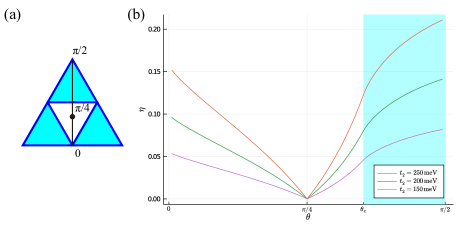
Figure 2: (a) Phase diagram of the Kitaev model Kitaev (2006). Cyan regions represent $A$ phase, and a white region represents $B$ phase. A black solid line represents the $K^{x}=K^{y}$ line, which is parametrized by $\theta$ as depicted. (b) $\eta$ with respect to the model parameter $\theta$. $\Delta=10$ meV, $\lambda=150$ meV, and $U=1.5$ eV are used. $t_{2}$ takes 150, 200, and 250 meV. Kitaev’s gapped $A$ phase is shown by a cyan shaded region.

Trigonal distortion.— Even if we introduce a small trigonal distortion $\Delta\neq 0$, the ground state remains a Kramers doublet in the atomic limit and the effective spin-1/2 description is valid. The effective operator form of EQM can be obtained almost in the same way as before up to the first order in $\Delta/\lambda$.

$$P_{0}q_{i}P_{0}= \begin{pmatrix}\frac{3it_{2}^{2}}{(U+\frac{3}{2}\lambda)^{2}}c_{i}c_{i_{x}}&-\frac{4\Delta}{3\lambda}&-\frac{4\Delta}{3\lambda}\\ -\frac{4\Delta}{3\lambda}&\frac{3it_{2}^{2}}{(U+\frac{3}{2}\lambda)^{2}}c_{i}c_{i_{y}}&-\frac{4\Delta}{3\lambda}\\ -\frac{4\Delta}{3\lambda}&-\frac{4\Delta}{3\lambda}&\frac{3it_{2}^{2}}{(U+\frac{3}{2}\lambda)^{2}}c_{i}c_{i_{z}}\end{pmatrix}$$

$$-\frac{t_{2}^{2}}{(U+\frac{3}{2}\lambda)^{2}}(ic_{i}c_{i_{x}}+ic_{i}c_{i_{y}}+ic_{i}c_{i_{z}})\openone_{3}$$

$$+O(\Delta^{2},\Delta t_{2}^{2},t_{2}^{4}).$$ (15)

By diagonalizing this tensor, we can calculate the value of $\eta$. Since usually $\Delta/\lambda>t_{2}^{2}/U^{2}$, the principal $a$-axis is nearly perpendicular to the (111) plane. $b$- and $c$-axes are inside this plane, detecting the $C_{3}$ symmetry of the system.

In order to show the relevance of our theory to detect NKSL, we try to check the size of $\eta$ for the ansatz state. In the mean-field level, the ansatz state of NKSL should be the ground state for the following ansatz Hamiltonian.

$$\mathcal{H}_{\textrm{NKSL}}=-\sum_{\langle ij\rangle\in\gamma}K^{\gamma}S_{i}^{\gamma}S_{j}^{\gamma},$$ (16)

where $K^{\gamma}>0$ is an effective Kitaev interaction for the $\gamma$-direction. On the $K^{x}=K^{y}$ line shown in Fig. 2(a), Lieb’s theorem Lieb (1994) is applicable and the expectation value of EQM becomes

$$\braket{\Psi_{\textrm{GS}}}{q_{i}}{\Psi_{\textrm{GS}}}=\braket{\Psi_{\textrm{GS}}}{P_{0}q_{i}P_{0}}{\Psi_{\textrm{GS}}},$$ (17)

for any ground state $\ket{\Psi_{\textrm{GS}}}$. We then compute $\eta$ for the ground state of $\mathcal{H}_{\textrm{NKSL}}$ along the line $K^{x}=K^{y}$. The results are shown in Fig. 2(b), where $\theta$ is defined as $\tan\theta=K^{z}/K^{x}$. The calculation method is included in SM SM .

From the isotropic point $\theta=\pi/4$ with $\eta=0$, the value of $\eta$ gradually grows, and continuously changes around $\theta=\theta_{\textrm{c}}$ with $\tan\theta_{\textrm{c}}=2$, where the topological transition between Kitaev’s $B$ and $A$ phases occurs. In the gapped $A$ phase (cyan shaded region), $\eta$ reaches 0.1–0.2. Thus, the topological nematic transition should result in $O(0.1)$ change of the value of $\eta$, which is definitely detectable in the Ru-NMR or Ru-MS measurement.

Though the transition is continuous, the derivative of $\eta$ has a cusp at the transition point (see Fig. S2 in SM SM ). Experimentally, the $B$ phase and the $A$ phase can be distinguished by the presence of a cusp in the derivative, and the critical value can be determined by its position. The consequence of an applied magnetic field is also discussed in SM SM .

Other contributions.— In this Letter, we have only considered the onsite $d$-orbital contribution to EFG. Usually, the interaction with EFG is divided into onsite and offsite contributions Abragam and Bleaney (1970) as $\mathcal{H}_{\textrm{el}}=\mathcal{H}_{\textrm{el}}^{\textrm{on}}+\mathcal{H}_{\textrm{el}}^{\textrm{out}}$ with

$$\mathcal{H}_{\textrm{el}}^{\textrm{on}} =-\frac{e^{2}Q}{2I(2I-1)}\langle r^{-3}\rangle\braket{L}{\!}{\alpha|\!|L}\bm{I}\tensor{q}\bm{I},$$

$$\mathcal{H}_{\textrm{el}}^{\textrm{out}} =(1-\gamma_{\infty})\frac{eQ}{2I(2I-1)}\bm{I}\tensor{V}^{\textrm{out}}\bm{I},$$ (18)

where $e$ is the elementary charge, $Q$ is the quadrupole moment of the nucleus, $\bm{I}$ are nuclear spin operators where $I$ depends on the isotope, $\langle r^{-3}\rangle$ is the expectation value of $r^{-3}$ for Ru $4d$-electrons, $\braket{L}{\!}{\alpha|\!|L}$ is a constant defined in Ref. Abragam and Bleaney (1970), $\gamma_{\infty}$ is the Sternheimer antishielding factor, and $\tensor{V}^{\textrm{out}}$ is the EFG tensor caused by the surrounding ions.

Usually, $\mathcal{H}_{\textrm{el}}^{\textrm{on}}$ is the main contribution as Ru $4d$-orbitals are strongly localized, and thus we have ignored the effect of $\mathcal{H}_{\textrm{el}}^{\textrm{out}}$ so far. However, because the $C_{3}$ symmetric structure of ligands is stable in $\alpha$-RuCl₃, the effect of $\tensor{V}^{\textrm{out}}$ is just renormalizing the value of $\Delta$. Therefore, our theory is qualitatively valid even if we include the contribution from the surrounding ions. Whether or not it gives a nonnegligible change quantitatively will be discussed in the future.

Discussion.— We have shown that the nematic transition in $\alpha$-RuCl₃ is detectable by NMR and MS through the measurement of $\eta$. Experiments should be combined with the high-resolution X-ray diffraction to exclude the possibility of a lattice distortion. While the conclusion is modified when the external magnetic field is applied, the first-order contribution vanishes and $\eta$ still serves as a nematic order parameter. The mechanism of the detection itself is different from conventional electronic nematic phases. Although the expression of $q$ given by the bilinear form of the spin operators is not limited to Kitaev systems, its highly anisotropic form is a consequence of the strong SOC.

Our theory can be generalized to the three-dimensional extensions of the Kitaev model O’Brien et al. (2016); Yamada et al. (2017b). Especially, the spin-Peierls instability expected in the hyperoctagon lattice Hermanns et al. (2015) is potentially detectable in our scheme based on NMR and MS.

In the case of NMR, not only static quantities like EFG, but also dynamical quantities can be observed. Especially, the nuclear spin-lattice relaxation rate divided by temperature $1/T_{1}T$ would also be a good probe for the time scale of the nematic transition. We would remark that the anisotropy of $1/T_{1}T$ can be another signature of the existence of a nematic order Smerald and Shannon (2016).