Self-consistency of optimizing finite-time Carnot engines with the low-dissipation model

Abstract

The efficiency at the maximum power (EMP) for finite-time Carnot engines established with the low-dissipation model, relies significantly on the assumption of the inverse proportion scaling of the irreversible entropy generation $\Delta S^{(\mathrm{ir})}$ on the operation time $\tau$, i.e., $\Delta S^{(\mathrm{ir})}\propto 1/\tau$. The optimal operation time of the finite-time isothermal process for EMP has to be within the valid regime of the inverse proportion scaling. Yet, such consistency was not tested due to the unknown coefficient of the $1/\tau$-scaling. In this paper, using a two-level atomic heat engine as an illustration, we reveal that the optimization of the finite-time Carnot engines with the low-dissipation model is self-consistent only in the regime of $\eta_{\mathrm{C}}\ll 1$, where $\eta_{\mathrm{C}}$ is the Carnot efficiency. In the large-$\eta_{\mathrm{C}}$ regime, the operation time for EMP obtained with the low-dissipation model is not within the valid regime of the $1/\tau$-scaling, and the exact EMP is found to surpass the well-known bound $\eta_{+}=\eta_{\mathrm{C}}/(2-\eta_{\mathrm{C}})$.

I Introduction

Converting heat into useful work, heat engine lies at the core of thermodynamics, both in classical and quantum regime (Huang, 2013; Tolman and Fine, 1948; Kosloff and Levy, 2014; Binder et al., 2018). Absorbing heat from a hot thermal bath with the temperature $T_{\mathrm{h}}$, the engine outputs work and releases part of the heat to the cold bath with the temperature $T_{\mathrm{c}}$. The upper limit of the heat engine working between two heat baths is given by the Carnot efficiency $\eta_{\mathrm{C}}=1-T_{\mathrm{c}}/T_{\mathrm{h}}$ (Huang, 2013). Due to the limitation of the quasi-static cycle with infinite-long operation time, the heat engine with Carnot efficiency generally has vanishing output power and in turn is of no practical use. To design the heat engine cycles operating in finite time, several practical heat engine models have been proposed (Andresen et al., 1984; Wu, 1999; Tu, 2012), such as the endo-reversible model (Reitlinger, 1929; Yvon, 1955; Chambadal, 1957; Novikov, 1958; Curzon and Ahlborn, 1975), the linear irreversible model (den Broeck, 2005; Wang and Tu, 2012; Izumida and Okuda, 2014), the stochastic model (Schmiedl and Seifert, 2008; Seifert, 2012), and the low-dissipation model (Esposito et al., 2010; Broeck, 2013; Holubec and Ryabov, 2015; Ma et al., 2018a; Gonzalez-Ayala et al., 2020; Abiuso and Perarnau-Llobet, 2020). The efficiency at maximum power (EMP), is proposed as an important parameter to evaluate the performance of these heat engines in the finite-time cycles.

The utilization of the low-dissipation model(Esposito et al., 2010; Broeck, 2013; Holubec and Ryabov, 2015; Ma et al., 2018a, b) simplifies the optimization of the finite-time Carnot-like heat engines. As the model assumption, the heat transfer between the engine and the bath in the finite-time quasi-isothermal process is divided into two parts as follow

$$Q_{\mathrm{h,c}}(\tau_{\mathrm{h}})=T_{\mathrm{h,c}}(\Delta S_{\mathrm{h,c}}-S_{\mathrm{h,c}}^{(\mathrm{ir})}),$$ (1)

where $\Delta S_{\mathrm{h}}=-\Delta S_{\mathrm{c}}=\Delta S$ is the reversible entropy change of the working substance and $S_{\mathrm{h,c}}^{(\mathrm{ir})}=\Sigma_{\mathrm{h,c}}/\tau_{\mathrm{h,c}}$ is the irreversible entropy generation which is inversely proportional to the process time $\tau_{\mathrm{\alpha}}$. Optimizing the output power $P(\tau_{\mathrm{h}},\tau_{\mathrm{c}})=[Q_{\mathrm{h}}(\tau_{\mathrm{h}})+Q_{\mathrm{c}}(\tau_{\mathrm{c}})]/(\tau_{\mathrm{h}}+\tau_{\mathrm{c}})$ with respect to the operation time $\tau_{\mathrm{h}}$ and $\tau_{\mathrm{c}}$, one gets the optimal operation times (Esposito et al., 2010) as

$$\tau_{\mathrm{h}}^{*} =\frac{2T_{\mathrm{h}}\Sigma_{\mathrm{h}}}{(T_{\mathrm{h}}-T_{\mathrm{c}})\Delta S}\left(1+\sqrt{\frac{T_{\mathrm{c}}\Sigma_{\mathrm{c}}}{T_{\mathrm{h}}\Sigma_{\mathrm{h}}}}\right),$$ (2)

$$\tau_{\mathrm{c}}^{*} =\frac{2T_{\mathrm{c}}\Sigma_{\mathrm{c}}}{(T_{\mathrm{h}}-T_{\mathrm{c}})\Delta S}\left(1+\sqrt{\frac{T_{\mathrm{h}}\Sigma_{\mathrm{h}}}{T_{\mathrm{c}}\Sigma_{\mathrm{c}}}}\right),$$ (3)

and the efficiency at the maximum power $\eta^{*}$ bounded by the following inequality as (Esposito et al., 2010; Tu, 2012)

$$\eta_{\mathrm{-}}\equiv\frac{\eta_{\mathrm{C}}}{2}\leq\eta^{*}\leq\frac{\eta_{\mathrm{C}}}{2-\eta_{\mathrm{C}}}\equiv\eta_{\mathrm{+}}.$$ (4)

Due to the simplicity of the model assumption and the universality of the obtained EMP, the low-dissipation model becomes one of the most studied finite-time heat engine models in recent years (Broeck, 2013; Holubec and Ryabov, 2015; Ma et al., 2018a; Gonzalez-Ayala et al., 2020; Abiuso and Perarnau-Llobet, 2020; Ma, 2020).

It is currently cleared that (Shiraishi et al., 2016; Cavina et al., 2017; Ma et al., 2018a, b, 2020) the low-dissipation assumption is valid in the long-time regime of $\tau_{\mathrm{h(c)}}/t_{\mathrm{r}}\gg 1$, where $t_{\mathrm{r}}$ is the relaxation time for the work substance to reach its equilibrium with the heat bath. And the dissipation coefficient $\Sigma_{\mathrm{h(c)}}$ of the $1/\tau$-scaling is determined by both the coupling strength $\gamma_{\mathrm{h(c)}}\sim 1/t_{\mathrm{r}}$ to the bath(Ma et al., 2018a, 2020) and the control scheme (Ma et al., 2018b, 2020). Such a relation implies that the condition $\tau_{\mathrm{h(c)}}^{*}/t_{\mathrm{r}}\gg 1$ is not fulfilled simply and should be justified to reveal the regime of validity. We check the consistency of the obtained EMP with a minimal heat engine model consisting of a single two-level system. In Sec. II, we analytically obtain the regime, where the optimal operation time to achieve EMP is consistent with the low-dissipation assumption. And we further show the possibility of the exact EMP of the engine to surpass the upper bound of EMP, i.e., $\eta_{\mathrm{+}}$, obtained with the low-dissipation model in the large-$\eta_{\mathrm{C}}$ regime in Sec. III.

II Self-consistency of the low-dissipation model in deriving efficiency at maximum power

The two-level atomic heat engine is the simplest quantum engine to demonstrate the relevant physical mechanisms (Geva and Kosloff, 1992; Quan et al., 2007; Su et al., 2018; Ma et al., 2018a, b). The energy spacing of the excited state $\left|e\right\rangle$ and ground state $\left|g\right\rangle$ is tuned by an outside agent to extract work with the Hamiltonian $H=\frac{1}{2}\hbar\omega\left(t\right)\sigma_{z},$ where $\sigma_{z}=\left|e\right\rangle\left\langle e\right|-\left|g\right\rangle\left\langle g\right|$ is the Pauli matrix in the z-direction. The Planck’s constant is taken as $\hbar=1$ in the following discussion for convenience. For the finite-time quasi-isothermal process with the duration $\tau$ of the two-level system, the low-dissipation assumption of the $1/\tau$ scaling is valid in the regime $\widetilde{\gamma}\tau\gg 1$ (Ma et al., 2018a), where $\widetilde{\gamma}=2\gamma T/\omega_{0}$. Here $\gamma$ is the coupling strength between the system and the bath with the temperature $T$ and $\omega_{0}$ is the initial energy spacing of the system during the process.

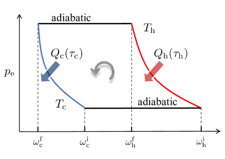
Figure 1: Schematic diagram of the finite-time Carnot-like cycle for a two-level atomic heat engine. The horizontal axis and the vertical axis represent respectively the energy spacing $\omega$ and excited state population $p_{\mathrm{e}}$ of the two-level atom. The red (blue) solid curve represents the high (low) temperature finite-time quasi-isothermal process, and the black solid lines represent the adiabatic processes.

The finite-time Carnot-like cycle for the two-level atomic heat engine of interest consists of four strokes, two isothermal and two adiabatic processes. The schematic diagram of the cycle is shown in Fig. 1. In the figure, $\omega_{\mathrm{h}}^{\mathrm{i}}$ and $\omega_{\mathrm{h}}^{\mathrm{f}}$ ($\omega_{\mathrm{c}}^{\mathrm{i}}$ and $\omega_{\mathrm{c}}^{\mathrm{f}}$ ) are respectively the initial and finial energy spacing of the working substance in the high (low) temperature finite-time quasi-isothermal process with duration $\tau_{\mathrm{h}}$ ($\tau_{\mathrm{c}}$), which is shown with the red (blue) solid curve. The total operating time per cycle is $t=\tau_{\mathrm{h}}+\tau_{\mathrm{c}}$. The interval of the adiabatic processes (the black solid lines) are ignored in comparison with $\tau_{\mathrm{h}}$ and $\tau_{\mathrm{c}}$ (Esposito et al., 2010; Ma et al., 2018a). We assume the two-level system has no energy level crossing during the whole cycle to ensure no coherence of the system is induced by non-adiabatic transition(Albash et al., 2012; Dann et al., 2018). The quasi-isothermal process retains the normal isothermal process at the quasi-static limit of $\tau_{\mathrm{h(c)}}\rightarrow\infty$.

For simplicity, we focus on the high-temperature regime, where the reversible entropy change $\Delta S_{\alpha}$ and the irreversible entropy generation coefficient $\Sigma_{\alpha}$ in Eq. (1) are analytically written as (Ma et al., 2018a)

$$\Delta S=\frac{\left[\left(\omega_{\mathrm{\alpha}}^{\mathrm{i}}\right)^{2}-\left(\omega_{\mathrm{\alpha}}^{\mathrm{f}}\right)^{2}\right]}{8T_{\mathrm{\alpha}}^{2}},\Sigma_{\alpha}=\frac{2\Delta S}{\widetilde{\gamma}_{\alpha}},$$ (5)

with $\alpha=\mathrm{h,c}$, and $\widetilde{\gamma}_{\alpha}=2\gamma_{\alpha}T_{\alpha}/\omega_{\mathrm{\alpha}}^{\mathrm{i}}$. Here and after, the Boltzmann’s constant $k_{\mathrm{B}}=1$ is chosen. To obtain the above equations, the relations $\omega_{\mathrm{h}}^{\mathrm{i}}/T_{\mathrm{h}}=\omega_{\mathrm{c}}^{\mathrm{f}}/T_{\mathrm{c}}$, $\omega_{\mathrm{h}}^{\mathrm{f}}/T_{\mathrm{h}}=\omega_{\mathrm{c}}^{\mathrm{i}}/T_{\mathrm{c}}$ have been used in the quantum adiabatic processes(Quan et al., 2007; Ma et al., 2018a). Substituting Eq. (5) into Eqs. (2) and (3), we obtain the corresponding optimal operation time $\tau_{\mathrm{\alpha}}^{*}$ for achieving the maximum power with the dimensionless time $\widetilde{\tau}_{\alpha}^{*}\equiv\tau_{\mathrm{\alpha}}^{*}\widetilde{\gamma}_{\alpha}$ as

$$\widetilde{\tau}_{\mathrm{h}}^{*}=\frac{2}{\eta_{\mathrm{C}}}\frac{\omega_{\mathrm{h}}^{\mathrm{i}}-\omega_{\mathrm{h}}^{\mathrm{f}}}{\omega_{\mathrm{h}}^{\mathrm{i}}+\omega_{\mathrm{h}}^{\mathrm{f}}}\left[1+\sqrt{\left(1-\eta_{\mathrm{C}}\right)\frac{\gamma_{\mathrm{h}}}{\gamma_{\mathrm{c}}}}\right],$$ (6)

$$\widetilde{\tau}_{\mathrm{c}}^{*}=\frac{2}{\eta_{\mathrm{C}}}\frac{\omega_{\mathrm{h}}^{\mathrm{i}}-\omega_{\mathrm{h}}^{\mathrm{f}}}{\omega_{\mathrm{h}}^{\mathrm{i}}+\omega_{\mathrm{h}}^{\mathrm{f}}}\left[\sqrt{\left(1-\eta_{\mathrm{C}}\right)\frac{\gamma_{\mathrm{c}}}{\gamma_{\mathrm{h}}}}+1-\eta_{\mathrm{C}}\right].$$ (7)

The low-dissipation assumption is valid in the regime $\widetilde{\tau}_{\mathrm{h}}^{*}\gg 1$ and $\widetilde{\tau}_{\mathrm{c}}^{*}\gg 1$, namely,

$$1+\sqrt{\left(1-\eta_{\mathrm{C}}\right)\frac{\gamma_{\mathrm{h}}}{\gamma_{\mathrm{c}}}}\gg\frac{\eta_{\mathrm{C}}}{2}\frac{\omega_{\mathrm{h}}^{\mathrm{i}}+\omega_{\mathrm{h}}^{\mathrm{f}}}{\omega_{\mathrm{h}}^{\mathrm{i}}-\omega_{\mathrm{h}}^{\mathrm{f}}}$$ (8)

$$\sqrt{\left(1-\eta_{\mathrm{C}}\right)\frac{\gamma_{\mathrm{c}}}{\gamma_{\mathrm{h}}}}+1-\eta_{\mathrm{C}}\gg\frac{\eta_{\mathrm{C}}}{2}\frac{\omega_{\mathrm{h}}^{\mathrm{i}}+\omega_{\mathrm{h}}^{\mathrm{f}}}{\omega_{\mathrm{h}}^{\mathrm{i}}-\omega_{\mathrm{h}}^{\mathrm{f}}}$$ (9)

The above two inequalities are fulfilled when

$$\eta_{\mathrm{C}}\ll 2\frac{1-\delta}{1+\delta},$$ (10)

where $\delta\equiv\omega_{\mathrm{h}}^{\mathrm{f}}/\omega_{\mathrm{h}}^{\mathrm{i}}$ is the compression ratio of the heat engine cycle in the quasi-isothermal process. The above relation is one of the main results of the current work and reveals the range of $\eta_{\mathrm{C}}$ in which the low-dissipation model is applicable for finding EMP. The bound for EMP obtained in the low-dissipation regime, as given by Eq. (4), thus may be not unconditionally applicable to such two-level atomic engine. Indeed, we will show the EMP out of the regime is larger than the upper bound $\eta_{+}$ predicted by the low-dissipation model in the next section.

III Efficiency at maximum power: beyond the low dissipation model

With the analytical discussion above, we find the EMP obtain with the low-dissipation model is only consistent with the assumption of the low-dissipation model in the low-$\eta_{\mathrm{C}}$ regime for the two-level system. The question is whether the bound provided by the low-dissipation model, i.e. $\eta_{+}$, is still the upper bound for the achievable efficiency of the system out of the low-$\eta_{\mathrm{C}}$ regime. Unfortunately, the answer is no. In this section, we will focus the efficiency at the maximum power in the regime with large $\eta_{\mathrm{C}}$.

By numerically simulating the dynamics of the two-level system engine with different cycle time, we obtain the exact power and efficiency to find the EMP. The results in the large-$\eta_{\mathrm{C}}$ regime show that: (i) the optimal operation time corresponding to the maximum power of the heat engine does not meet the low-dissipation assumption; (ii) the EMP surpass the upper bound obtained with the low-dissipation model, namely, $\eta_{\mathrm{MP}}>\eta_{+}$.

The dynamics of the two-level atom in the finite-time quasi-isothermal process is given by the master equation as follow (Ma et al., 2018a)

$$\frac{dp_{\mathrm{e}}(t)}{dt}=-\kappa(t)p_{\mathrm{e}}(t)+C(t),$$ (11)

where $p_{\mathrm{e}}(t)$ is the excited state population and $C(t)=\gamma n[\omega(t)]$. $\kappa(t)=\gamma\left(2n[\omega(t)]+1\right)$ is the effective dissipation rate with the mean occupation number $n[\omega(t)]=1/\left(\exp[\beta\omega(t)]-1\right)$ for the bath mode $\omega(t)$. The dissipation rate $\gamma$ equals to $\gamma_{\mathrm{h}}$ ($\gamma_{\mathrm{c}}$) in the high (low) temperature quasi-isothermal process with the inverse temperature $\beta=1/(k_{\mathrm{B}}T_{\mathrm{h}})$ ($\beta=1/(k_{\mathrm{B}}T_{\mathrm{c}})$). The energy spacing of the two-level atom is tuned linearly as $\omega(t)=\omega_{\mathrm{h}}^{\mathrm{i}}+(\omega_{\mathrm{h}}^{\mathrm{f}}-\omega_{\mathrm{h}}^{\mathrm{i}})t/\tau_{\mathrm{h}},\>t\in[0,\tau_{\mathrm{h}}]$ in the high-temperature finite-time quasi-isothermal process and as $\omega(t)=\omega_{\mathrm{c}}^{\mathrm{i}}+(\omega_{\mathrm{c}}^{\mathrm{f}}-\omega_{\mathrm{c}}^{\mathrm{i}})t/\tau_{\mathrm{c}},\>t\in[\tau_{\mathrm{c}},\tau_{\mathrm{c}}+\tau_{\mathrm{h}}]$ in the low-temperature finite-time quasi-isothermal process. The population of the two-level system keeps unchanged during the adiabatic processes whose operation time is ignored in comparison with $\tau_{\mathrm{h}}$ and $\tau_{\mathrm{c}}$.

In the following simulation, we set $\gamma_{\mathrm{h}}=1$ and focus on the regime of $\gamma_{\mathrm{c}}/\gamma_{\mathrm{h}}\rightarrow\infty$, i.e., $\Sigma_{\mathrm{c}}/\Sigma_{\mathrm{h}}\rightarrow 0$, where the upper bound $\eta_{+}=\eta_{\mathrm{C}}/(2-\eta_{\mathrm{C}})$ of EMP of the engine is achieved according to the prediction with the low-dissipation model(Esposito et al., 2010). In this regime, the low-temperature quasi-isothermal process approaches the isothermal process fastly enough that the operation time $\tau_{\mathrm{c}}$ is further ignored for the optimization of the cycle’s output power. The optimization is simplified as a single parameter optimization problem: find the maximum value $P_{\mathrm{max}}$ of the cycle’s output power with respect to $\tau_{\mathrm{h}}$, and obtain the EMP of the engine, $\eta_{\mathrm{MP}}\equiv\eta(P=P_{\mathrm{max}})$.

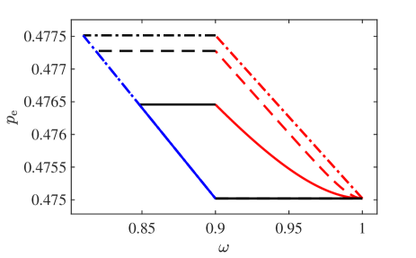
Figure 2: The finite-time Carnot-like cycles of for two-level atomic heat engine with different operation time $\tau_{\mathrm{h}}$. The red curves represent the high-temperature finite-time quasi-isothermal process with the duration $\tau_{\mathrm{h}}$, while the blue curves represent the low-temperature isothermal process . The adiabatic processes are plotted with the black lines. The outermost dash-dotted curves relate to the quasi-static cycle with $\tau_{\mathrm{h}}=200t_{\mathrm{r}}$, while the middle dashed cycle and inner solid cycle are obtained with $\tau_{\mathrm{h}}=10t_{\mathrm{r}}$ and $\tau_{\mathrm{h}}=2t_{\mathrm{r}}$, respectively. In this example, we choose $\omega_{\mathrm{h}}^{\mathrm{i}}=1$, $\omega_{\mathrm{h}}^{\mathrm{f}}=0.9$, $\gamma_{\mathrm{h}}=1$, $T_{\mathrm{h}}=10$, and $T_{\mathrm{c}}=9$. $t_{\mathrm{r}}=\omega_{\mathrm{h}}^{\mathrm{i}}/\left(2\gamma_{\mathrm{h}}T_{\mathrm{h}}\right)=0.05$ is the relaxation time related to the high-temperature finite-time quasi-isothermal process.

The cycles with different $\tau_{\mathrm{h}}$ are illustrated in Fig. 2, where $\omega_{\mathrm{h}}^{\mathrm{i}}=1$ and $\omega_{\mathrm{h}}^{\mathrm{f}}=0.9$ are fixed. The temperatures for the hot and cold bath are chosen as $T_{\mathrm{h}}=10$ and $T_{\mathrm{c}}=9$ as an example. The relaxation time is $t_{\mathrm{r}}=\omega_{\mathrm{h}}^{\mathrm{i}}/\left(2\gamma_{\mathrm{h}}T_{\mathrm{h}}\right)=0.05$. The quasi-static cycles with $\tau_{\mathrm{h}}=200t_{\mathrm{r}}$, $10t_{\mathrm{r}}$ and $2t_{\mathrm{r}}$ are represented by the dash-dotted line, dashed line, and solid line, respectively. The figure shows that the output work represented by the cycle area decreases with $\tau_{\mathrm{h}}$.

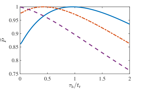
Figure 3: The normalized power of the engine $\widetilde{P}=P/P_{\mathrm{max}}$ as the function of $\tau_{\mathrm{h}}/t_{\mathrm{r}}$. The blue solid line, the orange dash-dotted line, and the purple dashed line are respectively obtained with $\eta_{\mathrm{C}}=0.1$, $\eta_{\mathrm{C}}=0.12$, and $\eta_{\mathrm{C}}=0.15$. In this example, we choose $\omega_{\mathrm{h}}^{i}=1$, $\omega_{\mathrm{h}}^{\mathrm{f}}=0.9$, $\gamma_{\mathrm{h}}=1$, and $T_{\mathrm{h}}=10$ with changing $T_{\mathrm{c}}=9$, $8.8$ and $8.5$. The relaxation time is $t_{\mathrm{r}}=\omega_{\mathrm{h}}^{\mathrm{i}}/\left(2\gamma_{\mathrm{h}}T_{\mathrm{h}}\right)=0.05$.

In Fig. 3, we show the normalized power of the engine $\widetilde{P}\equiv P/P_{\mathrm{max}}$ as the function of $\tau_{\mathrm{h}}/t_{\mathrm{r}}$ with $\eta_{\mathrm{C}}=0.1$ (blue solid line), $\eta_{\mathrm{C}}=0.12$ (orange dash-dotted line), and $\eta_{\mathrm{C}}=0.15$ (purple dashed line). In the simulation, the parameters are set as $\omega_{\mathrm{h}}^{i}=1$, $\omega_{\mathrm{h}}^{\mathrm{f}}=0.9$, and $T_{\mathrm{h}}=10$ with changing $T_{\mathrm{c}}=9$, $8.8$ and $8.5$. The relaxation time is $t_{\mathrm{r}}=0.05$. The maximum output power $P_{\mathrm{max}}$ is obtained numerically for different $\eta_{\mathrm{C}}$. It is observed from the figure that the dependence of $\widetilde{P}$ on operation time $\tau_{\mathrm{h}}$ changes with $\eta_{\mathrm{C}}$. In the figure, the optimal $\tau_{\mathrm{h}}^{*}$ decreases with $\eta_{\mathrm{C}}$ and is away from the low-dissipation regime of $\tau_{\mathrm{h}}/t_{\mathrm{r}}\gg 1$, illustrated with the orange dash-dotted line ($\eta_{\mathrm{C}}=0.12$, $\tau_{\mathrm{h}}^{*}/t_{\mathrm{r}}\approx 0.5$) and the blue solid line ($\eta_{\mathrm{C}}=0.1$, $\tau_{\mathrm{h}}^{*}/t_{\mathrm{r}}\approx 1$). As shown clearly by the purple dashed line with $\eta_{\mathrm{C}}=0.15$, the maximum power $\widetilde{P}=1$ is achieved in the short-time regime of $\tau_{\mathrm{h}}/t_{\mathrm{r}}\ll 1$, where the $1/\tau$-scaling of irreversible entropy generation is invalid (Ma et al., 2018a, 2020).

(a)

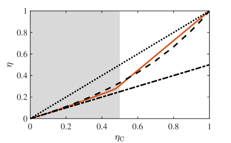
(b)

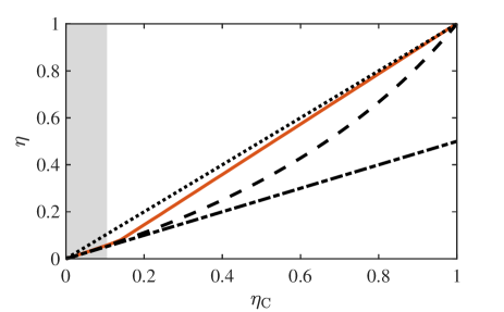
(c)

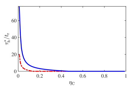
Figure 4: Efficiency at the maximum power $\eta_{\mathrm{MP}}$ (orange solid line) of the heat engine as the function of the Carnot efficiency $\eta_{\mathrm{C}}$ for different final energy spacing of the two level system(a) $\omega_{\mathrm{h}}^{\mathrm{f}}=0.6$ and (b) $\omega_{\mathrm{h}}^{\mathrm{f}}=0.9$. The black dashed line (black dash-dotted line) represents the upper bound $\eta_{\mathrm{+}}$ (lower bound $\eta_{\mathrm{-}}$) of EMP obtained with the low-dissipation model [Eq. (4)], and the Carnot efficiency $\eta_{\mathrm{C}}$ is plotted with the black dotted line. The gray area represents the low-dissipation regime predicted by Eq. (10). (c) Optimal operation time $\tau_{\mathrm{h}}^{*}$ at the maximum power as the function of $\eta_{\mathrm{C}}$. The blue solid curve is obtained with $\omega_{\mathrm{h}}^{\mathrm{f}}=0.6$ ($\delta=0.6$) while the red dash-dotted curve is obtained with $\omega_{\mathrm{h}}^{\mathrm{f}}=0.9$ ($\delta=0.9$). The other parameters in this figure are chosen as $\omega_{\mathrm{h}}^{\mathrm{i}}=1$, $\gamma_{\mathrm{h}}=1$, and $T_{\mathrm{h}}=10$. The relaxation time is $t_{\mathrm{r}}=\omega_{\mathrm{h}}^{\mathrm{i}}/\left(2\gamma_{\mathrm{h}}T_{\mathrm{h}}\right)=0.05$.

We show the obtained efficiency $\eta_{\mathrm{MP}}$ at the maximum power of the engine as the function of $\eta_{\mathrm{C}}$ in Fig. 4(a) and (b), and plot the corresponding optimal operation time $\tau_{\mathrm{h}}^{*}$ in Fig. 4(c). We choose the final energy spacing of the two level system as $\omega_{\mathrm{h}}^{\mathrm{f}}=0.6$ and $\omega_{\mathrm{h}}^{\mathrm{f}}=0.9$ respectively for (a) and (b), and other parameters are set as $\omega_{\mathrm{h}}^{\mathrm{i}}=1$, $\gamma_{\mathrm{h}}=1$, $T_{\mathrm{h}}=10$. As shown in Fig. 4(a) and (b), the EMP of the engine $\eta_{\mathrm{MP}}$(orange solid line) in the large-$\eta_{\mathrm{C}}$ regime surpasses the upper bound of EMP, $\eta_{+}=\eta_{\mathrm{C}}/(2-\eta_{\mathrm{C}})$ (black dashed line) obtained with the low-dissipation model. The lower bound of EMP, $\eta_{-}=\eta_{\mathrm{C}}/2$, obtained with the low-dissipation model is plotted with the black dash-dotted line. The gray area represents the consistent regime as demonstrated by Eq. (10).The figure shows that $\eta_{\mathrm{MP}}$ is bounded by $\eta_{+}$ and $\eta_{-}$ of Eq. (4) in the gray area with relatively small $\eta_{\mathrm{C}}$. Additionally, by comparing (b) and (a) of Fig. 4, with the larger the compression rate $\delta=\omega_{\mathrm{h}}^{\mathrm{f}}/\omega_{\mathrm{h}}^{\mathrm{i}}$ ($\delta=0.9$ for (a) and $\delta=0.6$ for (b)), we illustrate the narrower the range of $\eta_{\mathrm{C}}$ in which $\eta_{\mathrm{MP}}$ is bounded by $\eta_{+}$. With the increasing of the compression ratio $\delta$, the valid regime of optimization of the engine with the low-dissipation model becomes smaller. And it is consistent with the theoretical analysis of Eq. (10).

In Fig. 4(c), the optimal operation time $\tau_{\mathrm{h}}^{*}$ at the maximum power (blue solid curve for $\omega_{\mathrm{h}}^{\mathrm{f}}=0.6$ and red dash-dotted curve for $\omega_{\mathrm{h}}^{\mathrm{f}}=0.9$) decreases monotonically with increasing $\eta_{\mathrm{C}}$. The operation time at maximum power $\tau_{\mathrm{h}}^{*}$ of the engine is not in the low-dissipation regime of $\tau_{\mathrm{h}}/t_{\mathrm{r}}\gg 1$ for the relatively large $\eta_{\mathrm{C}}$. This explains why $\eta_{\mathrm{MP}}$ is no longer satisfies the bound provided by the low-dissipation model in large-$\eta_{\mathrm{C}}$ regime, and verifies our analytical analysis in Sec. II. In addition, one can find in Fig. 4(c) that the red dash-dotted curve is lower than the blue solid curve. This leads to a narrower parameter range of $\eta_{\mathrm{C}}$, in which the optimal operation time $\tau_{\mathrm{h}}^{*}$ satisfies the low-dissipation assumption, for the heat engine with $\omega_{\mathrm{h}}^{\mathrm{f}}=0.9$ than that with $\omega_{\mathrm{h}}^{\mathrm{f}}=0.6$. Therefore, the phenomenon that the gray area in Fig. 4(a) is wider than that in Fig. 4(b) is explained from the perspective of the operation time.

IV Conclusions and discussion

In summary, we checked whether the optimal operation time for achieving the maximum power is consistent with the requirement of the low-dissipation model for the finite-time Carnot-like heat engines in this paper. The low-dissipation model, widely used in the finite-time thermodynamics to study EMP, relies on the assumption that the irreversible entropy generation in the finite-time quasi-isothermal process of duration $\tau$ follows the $1/\tau$ scaling in the long-time regime. The operation time for the maximum power obtained from the model should fulfill the requirement of the low-dissipation model assumption. Due to the unknown coefficient of the $1/\tau$ scaling, the consistency of the model in optimizing finite-time Carnot engines had not been tested before.

In this paper, we proved that the optimal operation time for a two-level finite-time Carnot engine achieving EMP satisfy the low-dissipation assumption only in the low Carnot efficiency regime of $\eta_{\mathrm{C}}\ll 1$. This observation motivated us to check the EMP in the regime with large $\eta_{\mathrm{C}}$. We calculated the EMP of the two-level atomic heat engine in the full parameter space of $\eta_{\mathrm{C}}$. It is found that, in the large-$\eta_{\mathrm{C}}$ regime, the true EMP of the heat engine can surpass the upper bound for EMP, i.e., $\eta_{+}=\eta_{\mathrm{C}}/(2-\eta_{\mathrm{C}})$ obtained with the low-dissipation model.

Our study on EMP in the large-$\eta_{\mathrm{C}}$ regime shall provide a new insight for designing heat engines with better performance working between two heat baths with large temperature difference. In addition to affecting the EMP of the heat engine, the short-time effects caused by fast driving may also influence the trade-off between power and efficiency (Holubec and Ryabov, 2015; Shiraishi et al., 2016; Cavina et al., 2017; Ma et al., 2018a), which needs further exploration. The predictions of this paper can be tested on some experimental platforms (Martínez et al., 2015; Rossnagel et al., 2016; Deng et al., 2018; Albay et al., 2019; Ma et al., 2020; Bouton et al., 2020) in the short-time regime.