A Novel Reinitialization Scheme for Conservative Level Set Method

Abstract

Existing artificial compression based reinitialization scheme for conservative level set method has a few drawbacks, like distortion of fluid-fluid interface, unphysical patch formation away from the interface and lack of mass conservation. In this paper, a novel reinitialization approach has been presented which circumvents these limitations by reformulating the reinitialization equation. With the reformulated procedure, the present approach is able to reinitialize the level set function without causing any unwanted movement of the interface contour. The unphysical patch formation away from the interface is also resolved here by avoiding the use of ill-conditioned contour normal vectors. As a result of this measure, there is a significant improvement in the mass conservation property. In addition, the simplified form of the new reinitialization equation enables one to choose a much larger time step during the reinitialization iteration. Moreover, the new formulation also helps in reducing the amount of numerical computations per time step, leading to an overall reduction in the computational efforts. In order to evaluate the performance of the present formulation, a set of test problems involving reinitialization of stationary level set functions is carried out first. Then, the efficacy of the proposed reinitialization scheme is demonstrated using a set of standard two-dimensional scalar advection based test problems and incompressible two-phase flow problems. Finally, the ability to deal with complex mesh types is demonstrated by solving a test problem on an unstructured mesh consisting of finite volume cells having triangular and quadrilateral shapes.

Keywords: Multiphase flow; Finite volume method; Conservative level set method; Reformulation of reinitialization; Artificial compressibility method; Unstructured mesh.

Highlights

• Developed new reinitialization procedure by reformulating the artificial compression approach.

• Problems of interface movement and unphysical patch formation during reinitialization are completely resolved.

• Applicable to a wide variety of meshes including unstructured hybrid meshes and computationally efficient.

• Numerical results show superior mass conservation and good agreement with analytical and experimental results.

1 Introduction

Numerical simulation of incompressible two-phase flows poses great challenges due to the presence of the fluid-fluid interface. Popular contact capturing methods, such as, Volume of Fluid (VOF) method and Level Set (LS) method, use an additional interface advection equation along with the incompressible Navier-Stokes (NS) equations. Any inaccuracy in solving the interface advection equation will significantly affect the quality of the numerical solution. Issues of the formation of jetsam/ floatsam in VOF method, violation of mass conservation in LS method are a few examples associated with errors in the computation of the interface advection equation. In order to overcome the mass conservation error in the classical LS method, a variant of the LS method, known as Conservative Level Set (CLS) method, is proposed by Olsson and Kreiss [1] and Olsson et al [2]. The enhanced mass conservation property is achieved here by replacing the signed distance function used in the classical level set method with a hyperbolic tangent type level set function. This level set function is then advected using a scalar conservation law. In order to recover from the excessive numerical dissipation error, an artificial compression based reinitialization procedure is also formulated for the level set function. With the improved mass conservation property, the CLS method shows promising capabilities and provides a good alternative to the classical LS method in solving incompressible two-phase flow problems. However, in practice, the reinitialization procedure for level set function in CLS method often runs into various numerical difficulties, leading to undesirable results.

Primarily, two major issues with the reinitialization procedure are reported in the literature [3, 4, 5]. The first one is the undesired movement of the interface contour during reinitialization. The problem gets further aggravated with the frequent use of reinitialization. This issue arises particularly in two and three dimensions, where, the interface curvature gets involved in the computations. It is demonstrated in reference [3] that the degree of movement of interface contour depends upon the strength of the interface curvature. Also, a set of numerical experiments presented in reference [4] verifies that the frequent use of reinitialization results in substantial movement of the interface, leading to inaccuracies in the numerical solution. Several attempts to resolve this issue can be found in literature [6, 4]. The efforts are focused mainly on localizing the reinitialization process only to a selected region of the level set field. Excessive reinitialization at less dissipated regions is thus avoided. In reference [6], the reinitialization is localized by defining a local coefficient based on the degree of sharpness of the level set function. Whereas, in reference [4], a metric which depends on the local flow conditions and the numerical diffusion errors is used. It is, therefore, clear that these methods introduce additional complexity and computational efforts in obtaining the local coefficients.

The second issue of the original CLS method is the formation of unphysical fluid patches away from the interface due to the ill-conditioned behaviour of the interface contour normal vectors. The contour normal vectors decide the direction of the compression and diffusion fluxes during the reinitialization process. Far away from the fluid-fluid interface these contour normal vectors are expected to be zero, resulting in no reinitialization. However, due to their ill-conditioned nature, even far away from the interface the contour normal vectors may not necessarily be zero. This results in undesirable compression at far away region, which leads to formation of unphysical fluid patches there. Several cures for this problem can be found in literature [5, 3, 7, 8, 9, 10]. Most of the efforts are targeted towards replacing the ill-conditioned contour normal vectors with some alternatives. In the Accurate Conservative Level Set (ACLS) method, proposed in reference [5], the contour normal vectors are computed from an auxiliary signed distance function. The auxiliary signed distance function is constructed here from the level set function using a fast marching method. In the method proposed by Shukla et al. [3], a modified form of the reinitialization equation is used. Here, the level set function is replaced with a smooth function constructed from the level set function itself by employing a mapping procedure. A technique, by combining the reinitialization schemes of both the classical and conservative level set method, named as Improved Conservative Level Set (ICLS) Method, is reported in reference [7]. In reference [8] and its improved version in reference [9], reformulations of the original reinitialization equation are presented which take care of the spurious movement of interface contour as well as the ill-conditioned behaviour of the contour normal vectors. Recently in reference [10], the ill-conditioned unit contour normal vectors are replaced with another normal vectors, such that, their magnitudes start to diminish away from the interface. This ensures that the reinitialization process is activated only near the interface regions. Though improvements in the contour normal vectors partially circumvent the issue of formation of unphysical fluid patches, they involve evaluation of more complicated terms adding to the overall computational cost.

In the present work, a much simpler technique to reinitialize the level set function is presented. Here, the existing artificial compression based reinitialization equation is revised by isolating and removing terms that have potential to move the interface contours. The remaining terms in the modified equation are then reformulated considerably, such that, the usage of the contour normal vectors is completely avoided. With the new reformulation, issues such as, distortion of the interface contour and the unphysical patch formation away from the interface are resolved. As a consequence, the area conservation property is improved significantly. In addition, absence of a viscous dissipation like (second derivative) term in the new reinitialization equation enables one to choose a much larger time step during the reinitialization iteration. The simplified terms also help in significantly reducing the numerical computations per reinitialization time step, aiding an overall reduction in the computational efforts. In order to demonstrate the efficacy of the proposed reinitialization scheme, a set of standard two-dimensional test problems involving reinitialization of stationary level set functions (henceforth, we name it as in-place reinitialization problems), advection of level set function under predefined velocity fields and a few standard incompressible two-phase flow problems are solved. Finally, in order to demonstrate the ability to deal with complex mesh types, an incompressible two-phase flow problem is solved on an unstructured mesh consisting of finite volume cells having triangular and quadrilateral shapes.

Rest of the paper is organized as follows. The original CLS method and its reinitialization scheme is briefly described in section 2. The limitations of the existing artificial compression based reinitialization approach and its new reformulation are also discussed in the same section. In section 3, the mathematical formulation of incompressible two-phase flows is briefly described. The numerical discretization of the governing equations and the new reinitialization equation are also described in section 3. Several numerical test problems are solved in section 4. Finally the conclusions are given in section 5.

2 Conservative Level set Method

The fluid-fluid interface in conservative level set method is represented in the form of an iso-contour of a hyperbolic tangent type level set function, defined as,

$$\psi({\bf x},t)=\frac{1}{1+\exp\left(\frac{-\phi({\bf x},t)}{\varepsilon}\right)}\equiv\frac{1}{2}\left(\tanh\left(\frac{\phi({\bf x},t)}{2\varepsilon}\right)+1\right)$$ (1)

where, $\phi({\bf x},t)$ is the standard signed distance function defined in terms of the minimum distance $d({\bf x},t)$ from the interface, as,

$$\phi({\bf x},t)=\begin{cases}-d({\bf x},t),&\text{ inside the first fluid}\\ 0,&\text{ at the fluid-fluid interface}\\ +d({\bf x},t),&\text{ inside the second fluid}\end{cases}$$

The function $\psi$ takes a value $0$ at regions occupied by the first fluid and $1$ at the second fluid. Within a thin transition region between the two fluids, $\psi$ varies smoothly from $0$ to $1$. Width of the transition region is dictated by the parameter $\varepsilon$. The contour corresponds to $\psi({\bf x},0)=0.5$ represents the actual fluid-fluid interface. The geometric parameters associated with the interface, such as interface normal vector (${\bf n}$) and interface curvature (${\kappa}$), are obtained from the level set function as,

$${\bf n}=\frac{\nabla\psi}{\lvert\nabla\psi\rvert}$$ (2)

$$\kappa=-\nabla\cdot{\bf n}$$ (3)

Finally, movement of the fluid-fluid interface is achieved by advecting the level set function according to the flow field, as,

$$\frac{\partial\psi}{\partial t}+\nabla\cdot\left({\bf u}\psi\right)=0$$ (4)

where, ${\bf u}=u\hat{\text{i}}+v\hat{\text{j}}$, is the divergence-free velocity field.

2.1 Artificial Compression based Reinitialization Procedure

It is well known that the level set function suffers from excessive dissipation due to numerical errors [1]. This leads the level set function to deviate from its original hyperbolic tangent type profile. An artificial compression based reinitialization is developed in reference [2] in order to re-establish the pre-specified thickness and the profile of the level set function. The discretized level set advection equation together with the reinitialization should satisfy the following three requirements [1]. Firstly, the method should ensure discrete conservation of mass while advecting the level set function. Secondly, the method should not introduce any spurious oscillations. Finally, the initial properties of the level set function should be maintained throughout the simulation.

The equation for reinitializing the level set function can be written as per [2] as,

$$\frac{\partial\psi}{\partial\tau_{r}}+\nabla\cdot\left(\psi(1-\psi){\bf n}_{0}\right)-\nabla\cdot\left(\varepsilon\left(\nabla\psi\cdot{\bf n}_{0}\right)~{}{\bf n}_{0}\right)=0$$ (5)

where, ${\bf n}_{0}=\displaystyle\frac{\nabla\psi_{0}}{\lvert\nabla\psi_{0}\rvert}$ is the interface contour normal vector defined before the reinitialization starts. The variable $\tau_{r}$ is a time like variable and $\psi_{0}$ is the level set function defined at $\tau_{r}=0$. In equation (5), the second and third terms are responsible for the interface compression and diffusion respectively, which balances each other once the equation (5) converges in time $\tau_{r}$.

In practice, the reinitialization formulation suffers from various deficiencies. As described in the introduction, the above reinitialization procedure may involve error in the ${\bf n}_{0}$ computation. It may also be noted, the reinitialization equation moves the interface contour based on the local curvature. In order to identify terms that have potential to move the interface contour during the reinitialization, equation (5) is rewritten in non-conservative form by expanding the the compressive and diffusive terms. After rewriting equation (5) in non-conservative form, a curvature dependent velocity like term, ${\bf v}=\varepsilon\kappa_{0}\bigg{(}{\bf n}_{0}-\displaystyle\frac{\nabla\phi}{\lvert\nabla\phi\rvert^{2}}\bigg{)}$, is isolated which is found to be responsible for undesired movement of the interface (details shown in reference [11]).

2.2 Reformulation of the Reinitialization Equation

As described above, the curvature dependent advection term moves the interface; thus it is undesired in a reinitialization procedure. Therefore, in the new formulation of the reinitialization equation, we remove this curvature dependent advection term from the reinitialization equation. It may also be noted, the reinitialization equation is sensitive towards numerical errors arising from the ill-conditioned behaviour of the contour normal vectors. In order to overcome the difficulty to deal with the these terms, in the new formulation we seek for terms that are easy to compute and are less sensitive to numerical errors arising form the ill-conditioned contour normal vectors. After some manipulations (details shown in reference [11]), the final reformulated reinitialization equation can be written as,

$$\frac{\partial\psi}{\partial\tau_{n}}=-\psi(1-\psi)(1-2\psi)+\varepsilon(1-2\psi)\lvert\nabla\psi\rvert$$ (6)

It can be easily shown that the level set function, $\psi$, as given in equation (1), trivially satisfies the steady state form of equation (6). Furthermore, the overall behaviour of equation (6) can be described by considering each terms in the RHS individually. In the absence of the second term in RHS, equation (6) behaves like an ordinary differential equation with $\psi=1$ and $\psi=0$ as two stable equilibrium points and $\psi=0.5$ as an unstable equilibrium point. Figure 1 shows the phase plot of equation (6) with only first term in the RHS. From the phase plot, it is clear that the first term results in sharpening the level set function profile. Moreover, the first term also helps in stabilizing the overshoot ($\psi>1.0$) and undershoot ($\psi<0.0$) issues arising in case of the use of non-TVD numerical schemes for the original level set advection equation. Nature of the second term in the RHS of equation (6) is to balance the first term. Since the $\varepsilon$ and $\lvert\nabla\psi\rvert$ are always positive quantities, the sign of the second term depends on the sign of $(1-2\psi)$. That is, the sign of the second term is positive when $\psi<0.5$ and negative when $\psi>0.5$. At $\psi=0.5$, the second term is zero. In other words, the second term drives the level set function towards a flat profile with $\psi=0.5$ everywhere, thus balancing the first term. With the above mentioned sharpening and balancing actions, the equation (6) reinitializes the level set function.

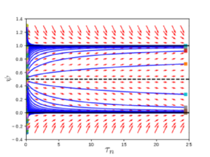
Figure 1: Phase plot for the new reinitialization equation. The arrows indicate the magnitude and direction of change of $\psi$ with respect to $\tau_{n}$. The blue lines show the trajectories of different initial values of $\psi$ as $\tau_{n}$ progresses. The initial and final values of $\psi$ are represented using circles and squares respectively.

3 Mathematical Formulation of Incompressible Two-Phase Flows

3.1 Governing Equations

A dual time-stepping based artificial compressibility approach is followed here for modelling incompressible two-phase flows. The governing system of equations describing the unsteady incompressible viscous two-phase flow can be written as,

$$\frac{\partial\bf U}{\partial\tau}+I^{t}\frac{\partial\bf U}{\partial t}+\left[\frac{\partial{\bf(F-F_{v})}}{\partial x}+\frac{\partial{\bf(G-G_{v})}}{\partial y}\right]={\bf F_{g}}+{\bf F_{s}}$$ (7)

where,

${\bf U}=\left\{\begin{array}[]{c}p/\beta\\ \rho u\\ \rho v\\ \psi\end{array}\right\}$; ${\bf F}=\left\{\begin{array}[]{c}u\\ \rho u^{2}+p\\ \rho uv\\ u\psi\end{array}\right\}$; ${\bf G}=\left\{\begin{array}[]{c}v\\ \rho uv\\ \rho v^{2}+p\\ v\psi\end{array}\right\}$; ${\bf F_{v}}=\left\{\begin{array}[]{c}0\\ 2\mu\frac{\partial u}{\partial x}\\ \mu(\frac{\partial u}{\partial y}+\frac{\partial v}{\partial x})\\ 0\end{array}\right\}$; ${\bf G_{v}}=\left\{\begin{array}[]{c}0\\ \mu(\frac{\partial u}{\partial y}+\frac{\partial v}{\partial x})\\ 2\mu\frac{\partial v}{\partial y}\\ 0\end{array}\right\}$; ${\bf F_{g}}=\left\{\begin{array}[]{c}0\\ -\rho g_{x}\\ -\rho g_{y}\\ 0\end{array}\right\}$;       ${\bf F_{s}}=\left\{\begin{array}[]{c}0\\ -\sigma\kappa\frac{\partial\psi}{\partial x}\\ \\ -\sigma\kappa\frac{\partial\psi}{\partial y}\\ 0\end{array}\right\}$;       $I^{t}=\left[\begin{array}[]{cccc}0&0&0&0\\ 0&1&0&0\\ 0&0&1&0\\ 0&0&0&1\\ \end{array}\right]$.

where, the vector ${\bf U}$ in equation (7) denotes the vector of conservative variables and the vectors $({\bf F},{\bf G})$ and $({\bf F_{v}},{\bf G_{v}})$ denote the convective and viscous flux vectors respectively. The vectors ${\bf F_{g}}$ and ${\bf F_{s}}$ denote the source terms containing gravitational and surface tension forces respectively. Here, the surface tension term is modelled using a continuum surface forces (CSF) method, proposed by Brackbill et al. [12]. The parameter $\sigma$ denotes the surface tension coefficient per unit length of interface and $g_{x}$ and $g_{y}$ denote the $x$ and $y$ components of the acceleration due to gravity. The variable $p$, $\rho$ and $\mu$ denote the pressure, density and dynamic viscosity of the fluid respectively. The variables $\tau$ and $t$ appearing in equation (7) denote the pseudo time and the real time respectively. The parameter $\beta$ denotes the artificial compressibility parameter, which is usually taken as constant for a given test problem. The artificial compressibility term added in the continuity equation is similar to the one introduced by Chorin in [13]. Once equation (7) converges to a pseudo-steady state, it recovers the set of unsteady incompressible two-phase flow equations. It can be noticed that the level set advection, described by equation(4), is combined here with the system of equations (7), and solved simultaneously along with the Navier-Stokes equations. The density and viscosity used in equation (7) are defined in terms of the level set function, as,

$$\rho=\rho(\psi)=\rho_{\text{2}}\psi+(1-\psi)\rho_{\text{1}}$$ (8)

$$\mu=\mu(\psi)=\mu_{\text{2}}\psi+(1-\psi)\mu_{\text{1}}$$ (9)

where the subscripts “1” and “2” indicate the properties corresponds to the first and the second fluids respectively.

3.2 Numerical Discretization of Governing Equations

A finite volume approach is followed here for solving the governing system of equations (7). In order to proceed with finite volume discretization, the governing system of equations (7) is first integrated over a control volume. The computational domain is then discretized into a finite number of non-overlapping finite volume cells. The final space discretized form of equations (7) for an $i^{\text{th}}$ finite volume cell can be written as,

$$\Omega_{i}\frac{\partial{\overline{\bf U}}}{\partial\tau}+I^{t}\Omega_{i}\frac{\partial{\overline{\bf U}}}{\partial t}+R\left({\overline{\bf U}}\right)=0$$ (10)

where,

$$R\left({\overline{\bf U}}\right)=\sum_{m=1}^{M}\left({\bf F}~{}n^{m}_{x}+{\bf G}~{}n^{m}_{y}\right)_{m}\Gamma_{m}-\sum_{m=1}^{M}\left({\bf F_{v}}~{}n^{m}_{x}+{\bf G_{v}}~{}n^{m}_{y}\right)_{m}\Gamma_{m}-\Omega_{i}{\overline{\bf F}_{g}}-\Omega_{i}{\overline{\bf F}_{s}},$$

$\Omega_{i}$ is the area, $\Gamma_{m}$ and ${\bf n}^{m}=(n^{m}_{x},n^{m}_{y})$ are the length and edge normals of the $m^{\text{th}}$ edge respectively and $M$ is the total number of edges of the finite volume cell $i$. The vectors ${\overline{\bf U}}$, ${\overline{\bf F}_{g}}$ and ${\overline{\bf F}_{s}}$ represent the cell averaged values of ${\bf U}$, ${\bf F_{g}}$ and ${\bf F_{s}}$ respectively. The source term vector, ${\bf\overline{F}_{g}}$, appearing in equation (10) is computed by multiplying the cell averaged value of density and the acceleration due to gravity. Evaluation of the surface tension vector, ${\overline{\bf F}_{s}}$, involves the computation of gradient, contour normal and curvature of the level set function. The contour normal and curvature are computed from the gradient of the level set function as per equation (2) and equation (3) respectively, where the gradient vector is evaluated using central least square method as explained in [14]. The convective flux vector $\left({\bf F}~{}n^{m}_{x}+{\bf G}~{}n^{m}_{y}\right)$ and the viscous flux vector $\left({\bf F_{v}}~{}n^{m}_{x}+{\bf G_{v}}~{}n^{m}_{y}\right)$ in equation (10) are computed at the edges of each cell using a Roe-type Riemann solver, developed in [15], and a Green-Gauss integral approach over a Coirier’s diamond path, described in [14], respectively. The real time derivatives appearing in equation (10) are computed using a three point implicit backward differencing procedure. Finally, an explicit three stage Strong Stability Preserving Runge-Kutta (SSP-RK) method, described in [16], is used for iterating in pseudo-time. The time step required for the pseudo-time iteration is computed by considering the convective, viscous and surface tension effects. For faster convergence, a local time stepping approach is adopted here, in which, each cell is updated using its own $\Delta\tau_{i}$. The local time step $\Delta\tau_{i}$ is computed as,

$$\Delta\tau_{i}=\text{min}(\Delta\tau^{\text{conv}}_{i},\Delta\tau^{\text{visc}}_{i},\Delta\tau^{\text{surf}}_{i})$$ (11)

where, $\Delta\tau^{\text{conv}}_{i},\Delta\tau^{\text{visc}}_{i}$ and $\Delta\tau^{\text{surf}}_{i}$ are the maximum allowed time steps due to convective flux, viscous flux and surface tension force respectively. These time steps are evaluated as,

$$\Delta\tau^{\text{conv}}_{i}=\frac{\nu~{}\Omega_{i}}{\sum_{m=1}^{M}\left(\lvert u_{n}\rvert+\sqrt{\left(u_{n}\right)^{2}+\frac{\beta}{\rho_{i}}}\right)_{m}\Gamma_{m}}\text{;}\Delta\tau^{\text{visc}}_{i}=\frac{\nu~{}\Omega_{i}^{2}}{\left(\frac{8}{3}\right)\frac{\mu_{i}}{\rho_{i}}\sum_{m=1}^{M}\left(\Gamma_{m}\right)^{2}}\text{ and }\Delta\tau^{\text{surf}}_{i}=\nu~{}\sqrt{\frac{(\rho_{1}+\rho_{2})h^{3}}{4\pi\sigma}}$$

where, $\nu$ is the Courant number, $h$ is the average cell size and $u_{n}$ is the velocity component along the edge normal direction. For stability reasons, the Courant number, $\nu$, is always taken less than unity. The $\Delta\tau_{i}$ computed using equation (11) is further restricted based on the real time step [17], as, $\Delta\tau_{i}\leq\frac{2}{3}\Delta t$. Detailed descriptions of the numerical methods used for solving incompressible two-phase flows are excluded from here due to brevity reasons. One can refer [15] and [14] for more details.

3.3 Numerical Discretization of Reinitialization Equation

The RHS of equation (6) consists of two terms. In order to evaluate the first term at a given cell, only the cell center values of $\psi$ is sufficient. However, evaluation of the second term involves computation of the gradient of $\psi$. Here, the gradient of $\psi$ at the cell centers are evaluated using a central least square approach discussed in A. Finally, the time integration of equation (6) is carried out using a three stage Strong Stability Preserving Runge-Kutta (SSP-RK-3) method described in section 3.3.1.

3.3.1 Time integration for the reinitialization equation

According to the SSP-RK-3 approach described in [16], the cell averaged value of the unknown function in equation (6) is updated as,

$$\begin{array}[]{r@{}l@{}l@{}l@{}l@{}l@{}l}\overline{\psi_{i}}^{1}&{}=&{}&{}&{}\overline{\psi_{i}}^{n}&{}+&{}\displaystyle\frac{\Delta\tau_{n}}{\Omega_{i}}~{}L\left({\overline{\psi_{i}}}^{n}\right)\\ \overline{\psi_{i}}^{2}&{}=\displaystyle\frac{3}{4}&{}\overline{\psi_{i}}^{n}&{}+\displaystyle\frac{1}{4}&{}\overline{\psi_{i}}^{1}&{}+\displaystyle\frac{1}{4}&{}\displaystyle\frac{\Delta\tau_{n}}{\Omega_{i}}~{}L\left({\overline{\psi_{i}}}^{1}\right)\\ \overline{\psi_{i}}^{n+1}&{}=\displaystyle\frac{1}{3}&{}\overline{\psi_{i}}^{n}&{}+\displaystyle\frac{2}{3}&{}\overline{\psi_{i}}^{2}&{}+\displaystyle\frac{2}{3}&{}\displaystyle\frac{\Delta\tau_{n}}{\Omega_{i}}~{}L\left({\overline{\psi_{i}}}^{2}\right)\end{array}$$ (12)

where, $\overline{\psi_{i}}^{n}$ and $\overline{\psi_{i}}^{n+1}$ are the cell averaged level set function defined at $n^{\text{th}}$ and $(n+1)^{\text{th}}$ time levels respectively, $\overline{\psi_{i}}^{1}$ and $\overline{\psi_{i}}^{2}$ are the intermediate values of $\psi$ and $L\left({\overline{\psi_{i}}}^{*}\right)=-\overline{\psi_{i}}^{*}(1-\overline{\psi_{i}}^{*})(1-2\overline{\psi_{i}}^{*})+\varepsilon\lvert\nabla\overline{\psi_{i}}^{*}\rvert(1-2\overline{\psi_{i}}^{*})$. For the explicit time integration of equation (6), the time step is restricted based on the nature of the reinitialization equation. In order to find out the allowable time step, equation (6) is rewritten in a Hamilton-Jacobi form with a velocity like variable, ${\bf\mathcal{S}}=\varepsilon(1-2\psi)\left(\frac{1-\lvert\nabla\phi\rvert}{\lvert\nabla\phi\rvert}\right){\bf n}$. Since the solution variable $\psi$ is updated according to the sharpening velocity vector ${\bf\mathcal{S}}$, a stable explicit time integration scheme for equation (6) is possible only with a restricted time step,

$$\Delta\tau_{n}\leq 2h^{d}$$ (13)

It may be noticed that the time step, $\Delta\tau_{n}$, given in equation (13) is larger by a factor of $4/h$ in comparison with the allowable time step for the artificial compression based reinitialization procedure [1]. Presence of a viscous dissipation term in the artificial compression based approach restricts the reinitialization time step to a smaller value [1].

4 Numerical Experiments

Performance of the new reinitialization procedure is evaluated using three types of test problems. In order to illustrate the movement of the interface contour during the reinitialization, a set of test problems involving reinitialization of stationary level set function, is carried out first in section 4.1. These problems are named here as in-place reinitialization problems. Followed to the in-place reinitialization problems, a set of scalar advection based test problems are considered in section 4.2, where, the area and shape errors during the level set advection are quantified. In the sections 4.3 - 4.5, several incompressible two-phase flow test problems are presented. These problems are arranged according to their increasing levels of complexities, starting from an inviscid flow problem to problems involving viscous and surface tension forces. All test problems are solved on simple Cartesian type meshes. However, in order to demonstrate the the ability to deal with complex mesh types, the last test problem is also solved on an unstructured mesh consisting of finite volume cells having triangular and quadrilateral shapes.

4.1 In-Place Reinitialization Problems

As illustrated in section 2.1, the reinitialization scheme often results in moving the interface contour according to the sign and strength of the interface curvature. In order to demonstrate this, a set of test problems involving reinitialization of stationary level set function, similar to the one reported in [9], is carried out here. In order to perform in-place reinitialization tests, a level set function, corresponds to some given geometry, is constructed first. For the present study, three standard shapes, namely, a circle with diameter of 4 units, an ellipse with 4 units and 2 units of major and minor axes respectively and a square with size 3 units, are chosen. The geometric shapes are placed at the center of a computational domain of square shaped region bounded between $-5\leq x\leq 5$ and $-5\leq y\leq 5$. The computational domain is discretized using a $200\times 200$ Cartesian mesh. The level set function corresponds to the given shape is then taken as the initial condition for the reinitialization equation and carried out large number of pseudo-time iterations. Under ideal situations, the reinitialization process should not result in movement of the interface contour. However, due to errors in the reinitialization scheme, this need not be satisfied always. Moreover, unlike other test problems, numerical errors associated with the advection of level set function are not present here. Therefore, these tests help in isolating the errors associated with only the reinitialization process.

In the present study, the original CLS reinitialization algorithm, described in [2], and the newly proposed reinitialization algorithm are compared. The deformation of the interface contour in both the cases are monitored constantly during the pseudo-time iterations. Figure 2, 3 and 4 show the interface contours during the in-place reinitialization compared with the initial contours in case of the circle, ellipse and square shapes respectively. The solid black curve denotes the interface contour during reinitialization and the dashed black curve denotes the initial interface contour. One can notice that, for all the three shapes, up to 10 number of reinitialization iterations no significant changes in the interface contours are visible. However, as the number of reinitialization iterations increases, the original CLS approach leads to interface contour deformations. Especially, more deformations can be observed at regions having higher curvature. Whereas, there are no visible deformations of the interface contours even after 250 iterations in case of the new reinitialization approach. This observation is in well agreement with the discussion given in section 2.1 and 2.2.

(a) CLS-Olsson (no.iter = 0)

(b) CLS-Olsson (no.iter = 10)

(c) CLS-Olsson (no.iter = 100)

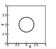
(d) CLS-Olsson (no.iter = 250)

(e) New (no.iter = 0)

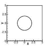
(f) New (no.iter = 10)

(g) New (no.iter = 100)

(h) New (no.iter = 250)

Figure 2: In-place reinitialization of a circular interface using the original CLS approach (a) to (d) and the new approach (e) to (h). The dashed black curve denotes the initial interface and the solid black curves denote the interfaces at the respective pseudo-time iterations.

(a) CLS-Olsson (no.iter = 0)

(b) CLS-Olsson (no.iter = 10)

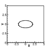
(c) CLS-Olsson (no.iter = 100)

(d) CLS-Olsson (no.iter = 250)

(e) New (no.iter = 0)

(f) New (no.iter = 10)

(g) New (no.iter = 100)

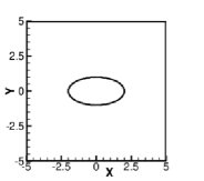
(h) New (no.iter = 250)

Figure 3: In-place reinitialization of an elliptical interface using the original CLS approach (a) to (d) and the new approach (e) to (h). The dashed black curve denotes the initial interface and the solid black curves denote the interfaces at the respective pseudo-time iterations.

(a) CLS-Olsson (no.iter = 0)

(b) CLS-Olsson (no.iter = 10)

(c) CLS-Olsson (no.iter = 100)

(d) CLS-Olsson (no.iter = 250)

(e) New (no.iter = 0)

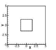
(f) New (no.iter = 10)

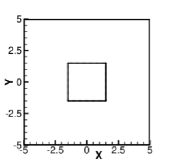
(g) New (no.iter = 100)

(h) New (no.iter = 250)

Figure 4: In-place reinitialization of a square shaped interface using original CLS approach (a) to (d) and the the new approach (e) to (h). The dashed black curve denotes the initial interface and the solid black curves denote the interfaces at the respective pseudo-time iterations.

4.2 Reinitialization of Scalar Advection Problems

In order to further study the performance of the new reinitialization formulation, a set of standard two-dimensional scalar advection based test problems are considered next. In the scalar advection problems, the initial interface is placed at $(0.25,~{}0.5)$ on a unit square domain and advected upon a predefined velocity field. Simulations are carried out till the initial interface completes one full rotation. The area confined by the interface and the $L^{1}$ and $L^{2}$ error norms are monitored during the simulation. The percentage area error, at any given time $t$, is computed as,

$$\text{Area Error (\%)}=\Bigg{(}\frac{A^{t}-A^{0}}{A^{0}}\Bigg{)}\times 100$$ (14)

where, $A$ is the area enclosed by the 0.5 contour of the level set function and the superscript $t$ and $0$ represent the data computed at time $t$ and at the initial time, $t=0$, respectively. Similarly, the $L^{1}$ and $L^{2}$ error norms are defined as,

$$L^{1}=\left(\frac{1}{Nx\times Ny}\right)\sum_{i=1}^{Nx}\sum_{j=1}^{Ny}\lvert\psi^{2\pi}_{ij}-\psi^{0}_{ij}\rvert$$ (15)

and

$$L^{2}=\left(\frac{1}{Nx\times Ny}\right)\sqrt{\sum_{i=1}^{Nx}\sum_{j=1}^{Ny}\Big{(}\psi^{2\pi}_{ij}-\psi^{0}_{ij}\Big{)}^{2}}$$ (16)

where, $\psi^{2\pi}_{ij}$ and $\psi^{0}_{ij}$ are the discretized level set functions defined at time level $t=2\pi$ and $t=0$ respectively, and $Nx$ and $Ny$ are the total number of cells along $x$ and $y$ directions respectively. In this section, the test problems are solved using the reinitialization schemes reported in [2, 5, 8, 9] along with the new scheme. For better clarity, the schemes are denoted here as CLS-Olsson, ACLS-Desjardins, CLS-Wacławczyk and CLS-Chiodi for references [2], [5], [8] and [9] respectively.

4.2.1 Reinitialization of circular disc rotation problem

Rotation of a circular disc, similar to the test reported in [1], is considered first, where, a circular disc of radius 0.15 units is advected upon a velocity field $u=(y-0.5)$ and $v=(0.5-x)$. Test problem is solved on four levels of Cartesian meshes starting from $25\times 25$ up to $200\times 200$. The level set contours correspond to $\psi=0.05,\psi=0.5$ and $\psi=0.95$ for the $100\times 100$ case at time levels $t=0$, $t=\pi/4$, $t=\pi/2$ and $t=3\pi/4$ for all five reinitialization schemes are plotted in Figure 5. Further, Table 1 and 2 show the percentage area error and error norms computed after the disc completes one full rotation ($ie.,$ at $t=2\pi$). Moreover, the error norms are plotted against the mesh size in Figure 6 along with reference slopes for the first and second order rate of convergence. Looking at the above figures and tables, it can be noticed that the new reinitialization shows the least error among all.

(a) CLS-Olsson

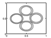
(b) ACLS-Desjardins

(c) CLS-Wacławczyk

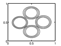
(d) CLS-Chiodi

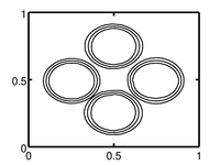
(e) New

Figure 5: Comparison of reinitialization schemes for the reinitialization of circular disc rotation problem solved on $100\times 100$ grid. Each subfigure shows the 0.05, 0.5 and 0.95 level contours of the level set functions at time levels of 0, $\pi$/4, $\pi$/2 and $3\pi$/4 (left, top, right and bottom respectively).

Table 1: Percentage area errors computed after completion of one full rotation of different reinitialization schemes for the reinitialization of circular disc rotation problem.

	Reinitialization Schemes
Mesh	CLS-Olsson	ACLS-Desjardins	CLS-Wacławszyk	CLS-Chiodi	New
$25\times 25$	-5.48500	-5.04690	-4.38460	-4.41610	-1.95050
$50\times 50$	-2.21890	-2.12190	-2.15960	-2.03820	-0.15707
$100\times 100$	-1.99710	-1.94980	-1.91780	-1.74080	-0.02158
$200\times 200$	-1.71600	-1.68580	-1.71300	-1.65980	-0.00865

Table 2: The $L^{1}$ and $L^{2}$ error norms of different reinitialization schemes for the reinitialization of circular disc rotation problem.

		Reinitialization Schemes
Errors	Mesh	CLS-Olsson	ACLS-Desjardins	CLS-Wacławszyk	CLS-Chiodi	New
	$25\times 25$	2.6488E-02	2.3154E-02	2.1835E-02	1.9378E-02	1.4665E-02
	$50\times 50$	5.2915E-03	5.4820E-03	5.2766E-03	5.5800E-03	5.5977E-03
	$100\times 100$	3.3020E-03	3.3816E-03	3.3176E-03	3.4732E-03	2.4589E-03
$L^{1}$ Error	$200\times 200$	2.1747E-03	2.2122E-03	2.1747E-03	2.2454E-03	1.2175E-03
	$25\times 25$	3.5611E-03	2.8689E-03	2.4137E-03	2.4929E-03	2.4929E-03
	$50\times 50$	4.4320E-04	4.4905E-04	4.3691E-04	4.4555E-04	4.4555E-04
	$100\times 100$	1.6393E-04	1.6817E-04	1.6307E-04	1.6827E-04	1.6827E-04
$L^{2}$ Error	$200\times 200$	7.3160E-05	6.9776E-05	7.4308E-05	6.9736E-05	6.9736E-05

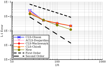
(a) $L^{1}$ Error

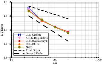
(b) $L^{2}$ Error

Figure 6: Convergence of the $L^{1}$ and $L^{2}$ error norms for the reinitialization of circular disc rotation problem solved on four ($25\times 25$, $50\times 50$, $100\times 100$ and $200\times 200$) grid levels.

4.2.2 Reinitialization of Zalesak’s disc rotation problem

The second problem considered is the advection of Zalesak’s disc, similar to the test reported in [5]. The Zalesak’s disc is of radius 0.15 units, and notch length and width of 0.3 units and 0.1 units respectively. Due to the presence of sharp corners, this test problem shows more numerical errors compared to the previous problem. Similar to the rotation of circular disc problem, this problem also is solved on four levels of Cartesian meshes starting from $25\times 25$ up to $200\times 200$. The level set contours correspond to $\psi=0.05,\psi=0.5$ and $\psi=0.95$ for the $100\times 100$ case at time levels $t=0$, $t=\pi/4$, $t=\pi/2$ and $t=3\pi/4$ for all five reinitialization schemes are plotted in Figure 7. Further, Table 3 and 4 show the percentage area error and error norms computed after the disc completes one full rotation ($ie.,$ at $t=2\pi$). Moreover, the error norms are plotted against the mesh size in Figure 8 along with reference slopes for the first and second order rate of convergence. Similar to the previous problem, here also it can be seen that the new reinitialization scheme is having the least error among all.

(a) CLS-Olsson

(b) ACLS-Desjardins

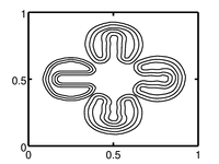
(c) CLS-Wacławczyk

(d) CLS-Chiodi

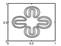
(e) New

Figure 7: Comparison of reinitialization schemes for the reinitialization of Zalesak’s disc rotation problem solved on $100\times 100$ grid. Each subfigure shows the 0.05, 0.5 and 0.95 level contours of the level set functions at time levels of 0.0, $\pi$/4, $\pi$/2 and $3\pi$/4 (left, top, right and bottom respectively).

Table 3: Percentage area errors after completion of one full rotation of different reinitialization schemes for the reinitialization of Zalesak’s disc rotation problem.

	Reinitialization Schemes
Mesh	CLS-Olsson	ACLS-Desjardins	CLS-Wacławszyk	CLS-Chiodi	New
$25\times 25$	-9.49000	-9.51580	-8.99110	-9.37870	-7.10470
$50\times 50$	-5.33530	-5.22570	-5.19310	-4.68600	-3.70040
$100\times 100$	-3.09830	-3.45670	-3.29800	-2.00520	-1.28230
$200\times 200$	-2.38510	-2.33920	-2.38360	-2.33040	-0.90177

Table 4: The $L^{1}$ and $L^{2}$ error norms of different reinitialization schemes for the reinitialization of Zalesak’s disc rotation problem.

		Reinitialization Schemes
Errors	Mesh	CLS-Olsson	ACLS-Desjardins	CLS-Wacławszyk	CLS-Chiodi	New
	$25\times 25$	4.2972E-02	3.9579E-02	4.1547E-02	3.6041E-02	1.9959E-02
	$50\times 50$	1.3590E-02	1.3860E-02	1.4083E-02	1.4145E-02	1.2202E-02
	$100\times 100$	7.4338E-03	7.6362E-03	7.4889E-03	7.8407E-03	6.4325E-03
$L^{1}$ Error	$200\times 200$	4.2656E-03	4.3188E-03	4.2485E-03	4.3666E-03	3.8105E-03
	$25\times 25$	5.5200E-03	4.8633E-03	4.6080E-03	4.6220E-03	2.4447E-03
	$50\times 50$	1.0000E-03	1.0103E-03	1.0334E-03	1.0402E-03	1.0036E-03
	$100\times 100$	3.7050E-04	3.8588E-04	3.7405E-04	3.9550E-04	3.8000E-04
$L^{2}$ Error	$200\times 200$	1.0556E-04	1.0664E-04	1.0473E-04	1.0647E-04	1.2000E-04

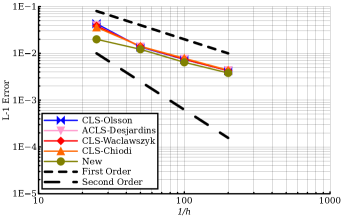
(a) $L^{1}$ Error

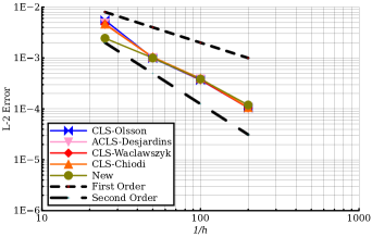
(b) $L^{2}$ Error

Figure 8: Convergence of the $L^{1}$ and $L^{2}$ error norms for the reinitialization of Zalesak’s disc rotation problem solved on four ($25\times 25$, $50\times 50$, $100\times 100$ and $200\times 200$) grid levels.

4.2.3 Reinitialization of circular disc deformation problem

The last scalar advection test problem considered is the advection of circular disc subjected to a shear velocity field, $u=\sin^{2}(\pi x)\sin(2\pi y)$, $v=-\sin^{2}(\pi y)\sin(2\pi x)$. Figure 9 shows a qualitative comparison of the interface contour for all five reinitialization scheme at $t=4$ s solved a $200\times 200$ Cartesian mesh. From Figure 9, one can clearly see that the tail of the interface is fully resolved without breaking in case of the new reinitialization scheme.

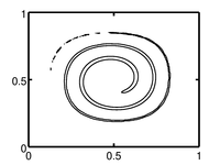
(a) CLS-Olsson

(b) ACLS-Desjardins

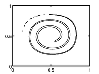
(c) CLS-Wacławczyk

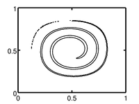
(d) CLS-Chiodi

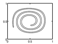
(e) New

Figure 9: Comparison of reinitialization schemes for the reinitialization of circular disc deformation problem solved on $200\times 200$ grid. Each subfigure shows the 0.5 level contours of the level set function at time levels of 4 s.

4.3 Broken Dam Problem

In previous sections, in-place reinitialization problems and scalar advection based test problems are solved. In order to compare its performance on more realistic problems, an inviscid broken dam problem, reported in [18, 15] is considered next. Here, an initial water column of height 0.9 m and width 0.45 m is kept at zero velocity field and subjected to a hydrostatic pressure distribution inside a computational domain bounded between $0\leq x\leq 2$ m and $0\leq y\leq 1$ m. The density of water and air are taken as 998.2 kg/m³ and 1.2040 kg/m³ respectively. The computational domain is discretized into $100\times 50$ Cartesian mesh. The artificial compressibility parameter, $\beta$, is taken as 10000. All four boundaries are set to free-slip boundary condition. As time progresses, due to the presence of gravitational force, the water column collapses. In order to accurately capture the interface movement, a small real-time step of 0.005 s is chosen. For stability reasons, a smaller Courant number of 0.1 is chosen for the computation of pseudo-time step.

Figure 10 shows the snapshots comparing the air-water interface computed using the CLS-Olsson and the new reinitialization procedure. One can see that the surge front, in case of the new reinitialization scheme, touches the top wall, then reaches the left wall and, finally, falls to the bottom pool of water. Since the free-slip wall boundary conditions do not offer any frictional resistance, such a behaviour is expected. However, in case of CLS-Olsson, the thin surge front is spoiled due to inaccuracies arising form the reinitialization scheme. One can see that, the surge front does not even touch the top wall. In order to compare the numerical results with experimental data reported in [19], the non-dimensional surge front, $s$, and non-dimensional water column height, $h$, are plotted with respect to the corresponding non-dimensional time scales $T_{s}=t\sqrt{2g/a}$ and $T_{h}=t\sqrt{g/a}$ respectively in Figure 11. The surge front and water column heights are non-dimensionalized with respect to their initial sizes. Looking at Figure 11, one can see an excellent match of both the numerical results with the experimental data reported by Martin and Moyce in [19]. Finally, Figure 12 shows the percentage area errors, computed using equation (14), with respect to time for both the cases. Clearly, the area loss is high for the CLS-Olsson case, especially during $t=1$ s, when the surge front becomes thin.

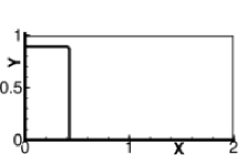
(a) CLS-Olsson ($t=0s$)

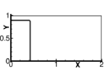
(b) New ($t=0s$)

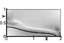
(c) CLS-Olsson ($t=0.5s$)

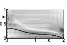
(d) New ($t=0.5s$)

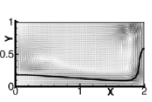
(e) CLS-Olsson ($t=0.75s$)

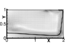
(f) New ($t=0.75s$)

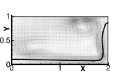
(g) CLS-Olsson ($t=1.0s$)

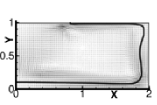
(h) New ($t=1.0s$)

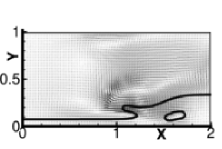
(i) CLS-Olsson ($t=1.5s$)

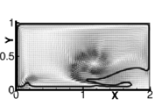
(j) New ($t=1.5s$)

Figure 10: Interface profiles at different time levels, starting from $t=0.0$ s up to $t=1.5$ s, for the broken dam problem. Subfigures (a), (c), (e), (g) and (i) correspond to the CLS-Olsson scheme and (b), (d), (f), (h) and (j) correspond to the new reinitialization scheme.

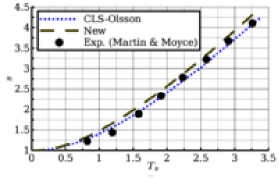
(a) $s$ versus $T_{s}$

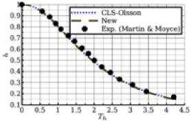
(b) $h$ versus $T_{h}$

Figure 11: The non-dimensional surge front and water column height plotted with respect to the corresponding non-dimensional time scales for the broken dam problem.

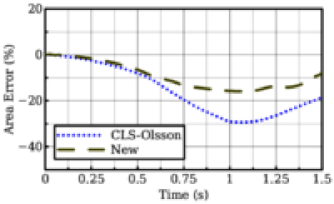
Figure 12: The percentage area error plotted with respect to time for the broken dam problem.

4.4 Rayleigh-Taylor Instability Problem

The second test problem considered is a Rayleigh-Taylor Instability problem similar to the one reported in [20, 15]. Unlike the previous problem, viscosity plays an important role here. In this problem, a heavier fluid of density 1.225 kg/m³ is placed on top of a lighter fluid of density 0.1694 kg/m³ inside the computational domain bounded between $0\leq x\leq 1$ and $0\leq y\leq 4$. The dynamic viscosity for both the fluids are taken to be the same, $\mu_{1}=\mu_{2}=3.1304952\times 10^{-3}$ kg/m s. The two fluids are initially separated by an interface, defined as, $y=2.0+0.05\cos(2\pi x)$. The problem is solved on a Cartesian mesh of $32\times 128$ finite volume cells. The top and bottom boundaries are set to no-slip boundary condition, whereas, the left and right boundaries are set as symmetric boundary condition. The initial velocity field is set to be zero and the pressure field is set based on gravity. The artificial compressibility parameter, $\beta$, is taken as 1000 and the real-time step is taken as 0.01 s. For stability reasons, the Courant number is chosen as 0.9 for the computation of the pseudo-time step.

As time progress, the top heavy fluid start to penetrate into the bottom light fluid resulting formation of an inverted mushroom shaped structure. Snapshots at different time levels during the evolution of the fluid-fluid interface for both the existing and new reinitialiation cases are shown in Figure 13. Similar to the previous problem, here also one can see that the new reinitialization scheme is better in capturing the thin fluid layer originating from the tips of the inverted mushroom head. Figure 14 compares the percentage area errors computed using equation (14) in both the cases. One can clearly see a higher area loss for the CLS-Olsson case during the later stages of interface evolution.

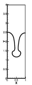
(a) ($t=0.8s$)

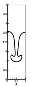
(b) ($t=0.9s$)

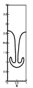
(c) ($t=1.0s$)

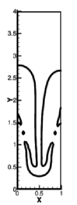
(d) ($t=1.2s$)

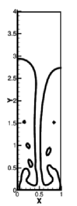
(e) ($t=1.4s$)

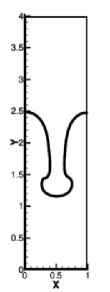
(f) ($t=0.8s$)

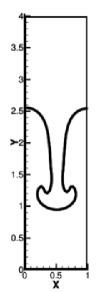
(g) ($t=0.9s$)

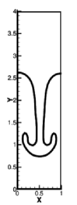
(h) ($t=1.0s$)

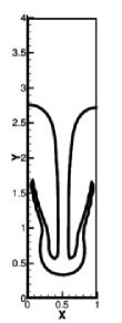
(i) ($t=1.2s$)

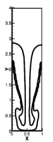
(j) ($t=1.4s$)

Figure 13: Interface profiles at different time levels, starting from $t=0.8$ s up to $t=1.4$ s, for the Rayleigh-Taylor instability problem. Subfigures from (a) to (e) correspond to the CLS-Olsson scheme and from (f) to (j) correspond to the new reinitialization scheme.

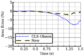
Figure 14: The percentage area error plotted with respect to time for the Rayleigh-Taylor instability problem.

4.5 Rising Bubble Problem

The last problem considered in this section is a rising bubble problem described in [21]. Unlike previous problems, this one is more challenging because of the presence of buoyancy, viscosity and surface tension forces. The problem consists of a circular bubble of diameter, $d_{b}=0.5$ m, placed at the lower half of a rectangular domain bounded between $0\leq x\leq 1$ m and $0\leq y\leq 2$ m, initially filled with a quiescent liquid. Due to the presence of the buoyant force, the initial circular bubble will start rising. With the interaction of the surrounding liquid, the initially circular shape of the bubble gets deformed. The degree of deformation of the circular bubble depends upon the Reynolds number ($Re$) and the Eötvös number ($Eo$). The $Re$ and $Eo$ are defined as,

$$Re=\frac{\rho_{2}U_{g}L}{\mu_{2}}$$ (17)

and

$$Eo=\frac{\rho_{2}U_{g}^{2}L}{\sigma}$$ (18)

where, the characteristic length scale, $L=d_{b}$, and the characteristic velocity scale, $U_{g}=\sqrt{gd_{b}}$. Based on the level of difficulty, two versions of rising bubble problems are reported in [21]. The first one (denoted here as “Case-1”) is relatively simple and the second one (denoted here as “Case-2”) is more challenging. The physical parameters defining the two dimensional rising bubble test cases are given in Table 5.

Table 5: Physical parameters defining the two dimensional rising bubble test cases.

Test case	$\rho_{2}$	$\rho_{1}$	$\mu_{2}$	$\mu_{1}$	$g$	$\sigma$	$Re$	$Eo$	$\rho_{2}/\rho_{1}$	$\mu_{2}/\mu_{1}$
Case-1	1000	100	10	1	0.98	24.5	35	10	10	10
Case-2	1000	1	10	0.1	0.98	1.96	35	125	1000	100

In both the cases, the initial velocity field is set to zero and the initial pressure field is set based on gravity. The left and right boundaries are set to free-slip boundary condition and the top and bottom walls are set to no-slip boundary condition. The artificial compressibility parameter, $\beta$, is taken as 10000. The real-time step is taken as 0.05 s and the pseudo-time step is computed according to the Courant number 0.9. Numerical simulations are carried out up to a time level of 4 s. In order to make a quantitative comparison, three parameters, namely, the rise velocity, the location of centroid and the circularity of the bubble are reported in [21]. These parameters are computed as,

$$\text{Rise Velocity, }{v_{c}}=\frac{\int_{\Omega_{b}}{\bf u}\cdot{\bf e}_{y}~{}\text{d}\Omega_{b}}{\int_{\Omega_{b}}\text{d}\Omega_{b}},$$ (19)

$$\text{Centroidal Location, }y_{c}=\frac{\int_{\Omega_{b}}{\bf x}_{b}\cdot{\bf e}_{y}~{}\text{d}\Omega_{b}}{\int_{\Omega_{b}}\text{d}\Omega_{b}}$$ (20)

and

$$\text{Circularity, }\zeta=\frac{P_{a}}{P_{b}}=\frac{\text{Perimeter of area-equivalent bubble}}{\text{Perimeter of the bubble}}=\frac{\pi d_{a}}{\int_{\Omega}\lVert\nabla\psi\rVert\text{d}\Omega}$$ (21)

where, $\Omega$ is the computational domain, $\Omega_{b}$ is the region occupied by the bubble, ${\bf x}_{b}$ is the position vector inside the bubble, ${\bf e}_{y}$ is the unit vector parallel to the $y-$axis and $d_{a}$ is the diameter of a circle with area equal to that of the bubble with circumference $P_{b}$.

4.5.1 Case-1

For the choice of physical parameters of Case-1, the bubble does not undergo large deformation. The initial circular bubble first stretches in the horizontal direction and, finally, settles down to an ellipsoidal profile as it reaches its terminal speed. Numerical simulations are carried out on a Cartesian mesh of $80\times 160$ finite volume cells. The bubble profiles at different time levels for both the CLS-Olsson and the new reinitialization cases are shown in Figure 15. One can see that the bubble profiles for the CLS-Olsson and the new reinitialization cases are quite similar and match very well with the results reported in [21]. In order to make a close comparison, the terminal shape of the bubbles in both the cases are plotted in Figure 16 along with the reference bubble profile of [21]. One can see from Figure 16 that the bubble profiles of both the CLS-Olsson and the new reinitialization schemes match very well with the reference bubble profile. The rise velocity, centroid location and the circularity of the rising bubble are plotted with respect to time in Figure 17. Here also, both the CLS-Olsson and the new reintialization results match closely with the reference plots. Finally, the percentage area error, computed using equation (14), is plotted with respect to time in Figure 18. It can be noticed that the area error is relatively less for the new reinitialization case compared to that of CLS-Olsson.

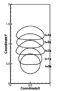
(a) CLS-Olsson

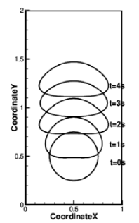
(b) New

Figure 15: Bubble profiles from $t=0$ s up to $t=4$ s for the rising bubble problem (Case-1).

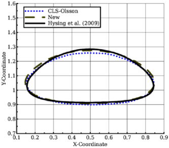
Figure 16: Enlarged bubble profiles at $t=3$ s for the rising bubble problem (Case-1).

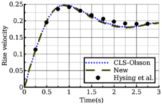
(a) Rise Velocity Vs Time

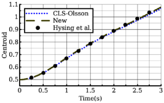
(b) Centroid Vs Time

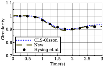
(c) Circularity Vs Time

Figure 17: The rise velocity, centroid location and circularity plotted with respect to time for the rising bubble problem (Case-1).

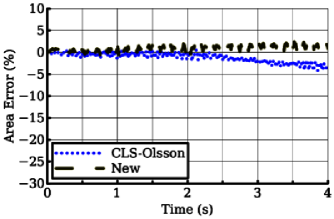
Figure 18: The percentage area error plotted with respect to time for the rising bubble problem (Case-1).

4.5.2 Case-2

Unlike the previous case, a large density ratio in this case results the bubble to deform more and acquire a dimple cap profile with thin elongated filament like structures originating from both sides. Due to the complex shape, it is relatively difficult to capture the bubble profile in Case-2 as compared to the Case-1. Numerical simulations are carried out on a Cartesian mesh of $80\times 160$ finite volume cells. Moreover, in order to demonstrate the ability of the new reinitialization scheme to deal with complex meshes, the problem is also solved on an unstructured mesh consisting of 23331 finite volume cells of triangular and quadrilateral shapes. Due to the clustering of cells in the bubble path, one may expect improved results in case of the unstructured mesh case. Figure 19 shows the Cartesian mesh and the unstructured meshes considered in this problem. The snapshots of bubble profiles at different time levels for all the three cases are shown in Figure 20. One can clearly see from Figure 20 that the elongated filament structure is not captured very well in case of the CLS-Olsson case. Whereas, a better profile of the elongated filament structure is captured in case of the new reinitialization method solved on the Cartesian mesh. The bubble profiles captured using the new reinitialization approach solved on unstructured mesh, however, show a close resemblance with the fine mesh results reported in [21]. The rise velocity, centroid location and circularity of the bubble are plotted with respect to time in Figure 21. One can see that the results for the new reinitialization scheme on the unstructured mesh show very good match with the reference results. Whereas, the results in case of CLS-Olsson, especially the circularity profile, are far away from the reference solution. Finally, the percentage area errors, computed using equation (14), are plotted in Figure 22. One can easily see that, the area error is highest for the CLS-Olsson case. The new reinitialization scheme solved on Cartesian mesh shows much less percentage area error. Whereas, the new reinitialization method solved on unstructured mesh shows the least area error.

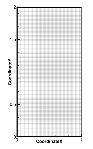
(a) Cartesian Mesh

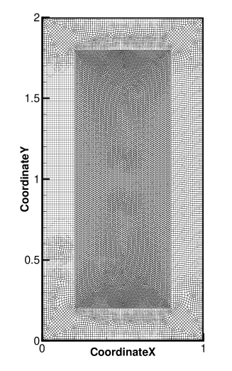
(b) Unstructured Mesh

Figure 19: The different meshes used for solving the rising bubble problem (Case-2). Subfigures (a) is the $80\times 160$ Cartesian mesh and (b) is the unstructured mesh consisting of 23331 finite volume cells of triangular and quadrilateral shape.

(a) ($t=0.0s$)

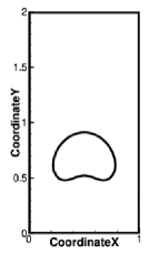
(b) ($t=1.0s$)

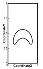
(c) ($t=2.0s$)

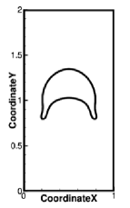
(d) ($t=3.0s$)

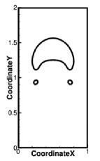
(e) ($t=4.0s$)

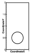
(f) ($t=0.0s$)

(g) ($t=1.0s$)

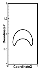
(h) ($t=2.0s$)

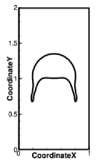
(i) ($t=3.0s$)

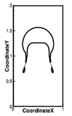
(j) ($t=4.0s$)

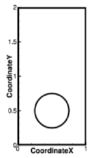
(k) ($t=0.0s$)

(l) ($t=1.0s$)

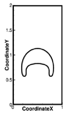
(m) ($t=2.0s$)

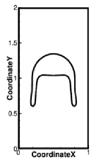
(n) ($t=3.0s$)

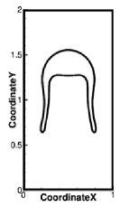
(o) ($t=4.0s$)

Figure 20: The bubble profiles at different time levels starting from $t=0$ s up to $t=4$ s for the rising bubble problem (Case-2). The subfigures from (a) to (e) correspond to the CLS-Olsson case computed on $80\times 160$ Cartesian mesh, from (f) to (j) correspond to the new reinitialization computed on $80\times 160$ Cartesian mesh and from (k) to (o) correspond to the new reinitialization computed on the unstructured mesh.

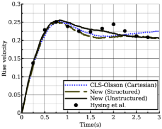
(a) Rise Velocity Vs Time

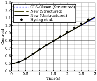
(b) Centroid Vs Time

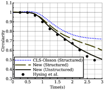
(c) Circularity Vs Time

Figure 21: The rise velocity, centroid location and circularity plotted with respect to time for the rising bubble problem (Case-2).

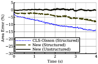
Figure 22: The percentage area error plotted with respect to time for the rising bubble problem (Case-2).

5 Conclusion

A new approach to reinitialize the level set function for the CLS method is formulated in this paper. The two major drawbacks of the existing artificial compression based reinitialization procedure, namely, the unwanted movement of the interface contour and strong sensitivity towards numerical errors leading to formation of unphysical fluid patches, are resolved with the new approach. Here, the existing artificial compression based reinitialization equation is first examined carefully in order to identify the term responsible for the movement of the interface contour. After isolating and removing a curvature dependent velocity term, that is responsible for moving the interface contour, the reinitialization equation is revised. The remaining terms in the reinitialization equation are then carefully replaced with equivalent terms that do not involve contour normal vectors. Unlike the compression and diffusion fluxes present in a typical artificial compression approach, the newly reformulated approach has a level set sharpening term, responsible for the narrowing the level set profile, and a balancing term in order to counteract the effect of sharpening. The combined effect of sharpening and balancing restores the level set function without causing any unwanted movement to the interface contour. Due to the absence of terms involving contour normal vectors, the susceptibility towards formation of unphysical fluid patches during reinitialization process has been completely eliminated in the new reinitialization procedure. As result of the new reinitialization approach, there has been significant improvement in the mass conservation property. While solving the new reinitialization equation, one can choose a larger time step, approximately by a factor of $4/h$, in comparison with the allowable time step of an artificial compression based approach. Moreover, the simplified terms also help in significantly reducing the numerical computation per reinitialization iteration, aiding an overall reduction in the computational efforts.

In order to evaluate the performance of the new reinitialization scheme, three types of numerical test cases are carried out. A set of in-place reinitialization problems demonstrate that the new reinitialization approach does not unnecessarily move the interface contour even after large number of reinitialization iterations. The area and shape errors of the new approach are quantified and compared against other reinitialization schemes using a set of scalar advection based test problems. In order to evaluate the performance on more practical problems, a set of standard incompressible two-phase flow problems, starting from an inviscid test case to complex test cases involving viscous and surface tension forces, are solved. Finally, in order to demonstrate the ability to deal with complex mesh types, an incompressible two-phase flow problem is also solved on an unstructured mesh consisting of finite volume cells having triangular and quadrilateral shapes. The numerical results of the incompressible two-phase flow problems show superior results as compared to the existing approach and match very well with the reference solutions reported in literature. With the enhanced accuracy and improved ability to deal with complex mesh types, the proposed reinitialization approach can be efficiently used in solving real life incompressible two-phase flow problems.

6 Acknowledgement

The present work is partially supported by Aeronautics Research & Development Board (AR&DB), with the project Grant number ARDB/01/1031930/M/I DT. 13.09.2019. We gratefully thank AR&DB for the support.

Appendix A Central least square estimation of level set gradients

The second term in equation (6) involves computation of level set gradient terms.

$$\lvert\nabla\psi\rvert_{i}=\sqrt{\left(\frac{\partial\psi}{\partial x}\right)_{i}+\left(\frac{\partial\psi}{\partial y}\right)_{i}}$$ (22)

These terms are evaluated here using central least square approach. In order to construct cell center derivatives, a stencil consisting of vertex based neighbours, as shown in Figure 23, is considered. Using Taylor series expansion, the neighbour cell values, $\psi_{j}$, of the level set function are expressed in terms of the value at cell $i$, as,

$$\psi_{j}=\psi_{i}+(x_{j}-x_{i})\left(\frac{\partial\psi}{\partial x}\right)_{i}+(y_{j}-y_{i})\left(\frac{\partial\psi}{\partial y}\right)_{i}\dots$$ (23)

where, $(x_{i},y_{i})$ and $(x_{j},y_{j})$ are locations of the centroids of cell $i$ and centroid of the neighbour cell $j$ respectively. Upon truncating the higher order terms (after the third order term) and re-arranging, equations (23) can be written as,

$$\Delta\psi={\bf S}~{}\text{d}\psi$$ (24)

where,

$\Delta\psi=\left\{\begin{array}[]{c}\psi_{1}-\psi_{i}\\ \psi_{2}-\psi_{i}\\ \dots\\ \dots\\ \psi_{l}-\psi_{i}\end{array}\right\}$;     ${\bf S}=\left[\begin{array}[]{cc}x_{1}-x_{i}&y_{1}-y_{i}\\ x_{2}-x_{i}&y_{2}-y_{i}\\ \dots&\dots\\ \dots&\dots\\ x_{l}-x_{i}&y_{l}-y_{i}\\ \end{array}\right]$;     $\text{d}\psi=\left\{\begin{array}[]{c}\displaystyle\frac{\partial\psi}{\partial x}\\ \\ \displaystyle\frac{\partial\psi}{\partial y}\\ \end{array}\right\}$

The overdetermined system of equation (24) can be solved as,

$$\text{d}\psi=\left({\bf S}^{\text{T}}{\bf S}\right)^{-1}{\bf S}^{\text{T}}\Delta\psi$$ (25)

Closed-form expressions for the derivatives can be obtained by simplifying equation (25) as,

$$\left(\frac{\partial\psi}{\partial x}\right)_{i}=\frac{\ell_{22}r_{1}-\ell_{21}r_{2}}{G}$$ (26a)

$$\left(\frac{\partial\psi}{\partial y}\right)_{i}=\frac{\ell_{11}r_{2}-\ell_{12}r_{1}}{G}$$ (26b)

where

$$\ell_{11}=\sum_{j=1}^{l}(x_{j}-x_{i})^{2},\hskip 14.22636pt\ell_{22}=\sum_{j=1}^{l}(y_{j}-y_{i})^{2},\hskip 14.22636pt\ell_{12}=\ell_{21}=\sum_{j=1}^{l}(x_{j}-x_{i})(y_{j}-y_{i})$$

$$r_{1}=\sum_{j=1}^{l}(x_{j}-x_{i})(\psi_{j}-\psi_{i}),\hskip 14.22636ptr_{2}=\sum_{j=1}^{l}(y_{j}-y_{i})(\psi_{j}-\psi_{i}),\hskip 14.22636ptG=\ell_{11}\ell_{22}-\ell_{12}^{2}$$

Figure 23: A schematic representation of a triangular shaped finite volume cell $i$ and its vertex based neighbours, denoted as $j$.

References

- [1] E. Olsson and G. Kreiss, “A conservative level set method for two phase flow,” Journal of Computational Physics, vol. 210, no. 1, pp. 225 – 246, 2005.
- [2] E. Olsson, G. Kreiss, and S. Zahedi, “A conservative level set method for two phase flow II,” Journal of Computational Physics, vol. 225, no. 1, pp. 785 – 807, 2007.
- [3] R. K. Shukla, C. Pantano, and J. B. Freund, “An interface capturing method for the simulation of multi-phase compressible flows,” Journal of Computational Physics, vol. 229, no. 19, pp. 7411 – 7439, 2010.
- [4] J. O. McCaslin and O. Desjardins, “A localized re-initialization equation for the conservative level set method,” Journal of Computational Physics, vol. 262, pp. 408 – 426, 2014.
- [5] O. Desjardins, V. Moureau, and H. Pitsch, “An accurate conservative level set/ghost fluid method for simulating turbulent atomization,” Journal of Computational Physics, vol. 227, no. 18, pp. 8395 – 8416, 2008.
- [6] Y. Sato and B. Ničeno, “A conservative local interface sharpening scheme for the constrained interpolation profile method,” International Journal for Numerical Methods in Fluids, vol. 70, no. 4, pp. 441–467, 2012.
- [7] L. Zhao, J. Mao, X. Bai, X. Liu, T. Li, and J. Williams, “Finite element implementation of an improved conservative level set method for two-phase flow,” Computers & Fluids, vol. 100, pp. 138 – 154, 2014.
- [8] T. Wacławczyk, “A consistent solution of the re-initialization equation in the conservative level-set method,” Journal of Computational Physics, vol. 299, no. Supplement C, pp. 487 – 525, 2015.
- [9] R. Chiodi and O. Desjardins, “A reformulation of the conservative level set reinitialization equation for accurate and robust simulation of complex multiphase flows,” Journal of Computational Physics, vol. 343, pp. 186 – 200, 2017.
- [10] N. Shervani-Tabar and O. V. Vasilyev, “Stabilized conservative level set method,” Journal of Computational Physics, vol. 375, pp. 1033 – 1044, 2018.
- [11] S. Parameswaran and J. C. Mandal, “A novel reinitialization scheme for conservative level set method,” Manuscript submitted for publication, vol. 00, pp. 000 – 000, 2020.
- [12] J. Brackbill, D. Kothe, and C. Zemach, “A continuum method for modeling surface tension,” Journal of Computational Physics, vol. 100, no. 2, pp. 335 – 354, 1992.
- [13] A. J. Chorin, “A numerical method for solving incompressible viscous flow problems,” Journal of Computational Physics, vol. 2, pp. 12 – 26, 1967.
- [14] S. Parameswaran and J. C. Mandal, “A conservative finite volume method for incompressible two-phase flows on unstructured meshes,” Manuscript submitted for publication, 2020.
- [15] S. Parameswaran and J. C. Mandal, “A novel Roe solver for incompressible two-phase flow problems,” Journal of Computational Physics, vol. 390, pp. 405 – 424, 2019.
- [16] S. Gottlieb, “On high order strong stability preserving runge-kutta and multi step time discretizations,” Journal of Scientific Computing, vol. 25, pp. 105–128, Oct. 2005.
- [17] A. L. Gaitonde, “A dual-time method for two-dimensional unsteady incompressible flow calculations,” International Journal for Numerical Methods in Engineering, vol. 41, no. 6, pp. 1153–1166, 1998.
- [18] Y. Aiming, C. Sukun, Y. Liu, and Y. Xiaoquan, “An upwind finite volume method for incompressible inviscid free surface flows,” Computers & Fluids, vol. 101, pp. 170 – 182, 2014.
- [19] J. C. Martin and W. J. Moyce, “Part IV. an experimental study of the collapse of liquid columns on a rigid horizontal plane,” Philosophical Transactions of the Royal Society of London A: Mathematical, Physical and Engineering Sciences, vol. 244, no. 882, pp. 312–324, 1952.
- [20] E. G. Puckett, A. S. Almgren, J. B. Bell, D. L. Marcus, and W. J. Rider, “A high-order projection method for tracking fluid interfaces in variable density incompressible flows,” Journal of Computational Physics, vol. 130, no. 2, pp. 269 – 282, 1997.
- [21] S. Hysing, S. Turek, D. Kuzmin, N. Parolini, E. Burman, S. Ganesan, and L. Tobiska, “Quantitative benchmark computations of two-dimensional bubble dynamics,” International Journal for Numerical Methods in Fluids, vol. 60, no. 11, pp. 1259–1288, 2009.