Separation of scales: Dynamical approximations for composite quantum systems

Abstract.

We consider composite quantum-dynamical systems that can be partitioned into weakly interacting subsystems, similar to system-bath type situations. Using a factorized wave function ansatz, we mathematically characterize dynamical scale separation. Specifically, we investigate a coupling régime that is partially flat, i.e., slowly varying with respect to one set of variables, for example, those of the bath. Further, we study the situation where one of the sets of variables is semiclassically scaled and derive a quantum-classical formulation. In both situations, we propose two schemes of dimension reduction: one based on Taylor expansion (collocation) and the other one based on partial averaging (mean-field). We analyze the error for the wave function and for the action of observables, obtaining comparable estimates for both approaches. The present study is the first step towards a general analysis of scale separation in the context of tensorized wavefunction representations.

1. Introduction

We consider composite quantum-dynamical systems that can be partitioned into weakly interacting subsystems, with the goal of developing effective dynamical descriptions that simplify the original, fully quantum-mechanical formulation. Typical examples are small reactive molecular fragments embedded in a large molecular bath, namely, a protein, or a solvent, all being governed dynamically by quite distinct energy and time scales. To this end, various régimes of intersystem couplings are considered, and a quantum-classical approximation is explored. A key aspect is dimension reduction at the wave function level, without referring to the conventional “reduced dynamics” approaches that are employed in system-bath theories.

1.1. The mathematical setting

The quantum system is described by a time-dependent Schrödinger equation

(1.1) $$i{\partial}_{t}\psi=H\psi\quad;\quad\psi_{\mid t=0}=\psi_{0},$$

governed by a Hamiltonian of the form

$$H=H_{x}+H_{y}+W(x,y),$$

where the coupling potential $W(x,y)$ is a smooth function, that satisfies growth estimates guaranteeing existence and uniqueness of the solution to the Schrödinger equation (1.1) for a rather general set of initial data, as we shall see later in Section 2. The overall set of space variables is denoted as $(x,y)\in{\mathbb{R}}^{n}\times{\mathbb{R}}^{d}$ such that the total dimension of the configuration space is $n+d$. The wave function depends on time $t\geqslant 0$ and both space variables, that is, $\psi=\psi(t,x,y)$. We suppose that initially scales are separable, that is, we work with initial data of product form

(1.2) $$\psi(0,x,y)=\psi_{0}(x,y)=\varphi_{0}^{x}(x)\varphi_{0}^{y}(y).$$

In the simple case without coupling, that is, $W\equiv 0$, the solution stays separated, $\psi(t,x,y)=\varphi^{x}(t,x)\varphi^{y}(t,y)$ for all time, where

$$i{\partial}_{t}\varphi^{x}=H_{x}\varphi^{x}\quad;\quad\varphi^{x}_{\mid t=0}=\varphi_{0}^{x},$$

$$i{\partial}_{t}\varphi^{y}=H_{y}\varphi^{y}\quad;\quad\varphi^{y}_{\mid t=0}=\varphi_{0}^{y},$$

and this is an exact formula. Here, we aim at investigating the case of an actual coupling with ${\partial}_{x}{\partial}_{y}W\not\equiv 0$ and look for approximate solutions of the form

$$\psi_{\rm app}(t,x,y)=\varphi^{x}(t,x)\varphi^{y}(t,y),$$

where the individual components satisfy evolution equations that account for the coupling between the variables. The main motivation for such approximations is dimension reduction, since $\varphi^{x}(t,x)$ and $\varphi^{y}(t,y)$ depend on variables of lower dimension than the initial $(x,y)$. Of crucial importance is the choice of the approximate Hamiltonian $H_{\rm app}=H_{x}+H_{y}+W_{\rm app}(t,x,y)$, that governs the approximate dynamics. We consider two different approximate coupling potentials: One is the time-dependent Hartree mean-field potential, the other one, computationally less demanding, is based on a brute force single-point collocation. Time-dependent Hartree methods have been known for a long time and have earned the reputation of oversimplifying the dynamics of real molecular systems. We emphasize, that our present study does not aim at rejuvenating but at deriving rigorous mathematical error estimates, which seem to be missing in the literature. Surprisingly, our error analysis provides similar estimates for both methods, the collocation and the mean-field approach. We investigate the size of the difference between the true and the approximate solution in the $L^{2}$-norm,

$$\|\psi(t)-\psi_{\rm app}(t)\|_{L^{2}}=\sqrt{\int_{{\mathbb{R}}^{n+d}}|\psi(t,x,y)-\psi_{\rm app}(t,x,y)|^{2}\,dxdy}$$

and in Sobolev norms. We present error estimates that explicitly depend on derivatives of the coupling potential $W(x,y)$ and on moments of the approximate solution. As an additional error measure we also consider the deviation of true and approximate expectation values $\left\langle\psi(t),A\psi(t)\right\rangle-\left\langle\psi_{\rm app}(t),A\psi_{\rm app}(t)\right\rangle$, for self-adjoint linear operators $A$. Roughly speaking, the estimates we obtain for observables depend on one more derivative of the coupling potential $W(x,y)$ than the norm estimates. This means that in many situations expectation values are more accurately described than the wave function itself. Even though rigorous error estimates that quantify the decoupling of quantum subsystems in terms of flatness properties of the coupling potential $W(x,y)$ are naturally important, our results here seem to be the first ones of their kind.

1.2. Relation with previous work

Interacting quantum systems have traditionally been formulated from the point of view of reduced dynamics theories, based on quantum master equations in a Markovian or non-Markovian setting [3]. More recently, also tensorized representations of the full quantum system have been considered, as for example by matrix product states (MPS) [33, 34] or within a multiconfiguration time-dependent Hartree (MCTDH) approach [5, 15, 29, 39]. Both wavefunctions (pure states) and density operators (mixed states) can be described in this framework, and wavefunction-based computations can be used to obtain density matrices [36]. In the chemical physics literature, dimension reduction for quantum systems has been proposed in the context of mean-field methods [14, 16], and the quantum-classical mean-field Ehrenfest approach [13, 2]. Also, quantum-classical formulations have been derived in Wigner phase space [27, 21] and in a quantum hydrodynamic setting [17, 6, 35]. Our present mathematical formulation circumvents formal difficulties of these approaches [10, 37, 32], by preserving a quantum wavefunction description for the entire system. Previous mathematical work we are aware of is concerned with rather specific coupling models, as for example the coupling of Hartree–Fock and classical equations in [7], or the time-dependent self-consistent field equations in [20], or with adiabatic approximations which rely on eigenfunctions for one part of the system, see for example [38, 28]. To the best of our knowledge, the rather general mathematical analysis of scale separation in quantum systems we are developing here is new.

1.3. Partially flat coupling.

For a first approximate potential, we consider a brute-force approach, where we collocate partially at a single point, for definiteness we choose the origin, and set

$$W_{\rm bf}(x,y)=W(x,0)+W(0,y)-W(0,0).$$

In comparison, following the more conventional time-dependent Hartree approach, we set

$$W_{\rm mf}(t,x,y)=\left\langle W\right\rangle_{y}(t,x)+\left\langle W\right\rangle_{x}(t,y)-\left\langle W\right\rangle(t),$$

where we perform partial and full averages of the coupling potential,

$$\left\langle W\right\rangle_{x}=\int_{{\mathbb{R}}^{d}}W(x,y)\,|\varphi^{x}(t,x)|^{2}\,dx\Big{/}\int_{{\mathbb{R}}^{d}}|\varphi^{x}(t,x)|^{2}\,dx,$$

$$\left\langle W\right\rangle_{y}=\int_{{\mathbb{R}}^{d}}W(x,y)\,|\varphi^{y}(t,y)|^{2}\,dy\Big{/}\int_{{\mathbb{R}}^{d}}|\varphi^{y}(t,y)|^{2}\,dy,$$

$$\left\langle W\right\rangle=\int_{{\mathbb{R}}^{n+d}}W(x,y)\,|\varphi^{x}(t,x)\varphi^{y}(t,y)|^{2}\,dxdy\Big{/}\int_{{\mathbb{R}}^{n+d}}|\varphi^{x}(t,x)\varphi^{y}(t,y)|^{2}\,dxdy.$$

For both approximations, the brute-force and the mean-field approximation, we derive various types of estimates for the error in $L^{2}$-norm. Our key finding is that both methods come with error bounds that are qualitatively the same, since they draw from either evaluations or averages of the function

$$\delta W(x,x^{\prime},y,y^{\prime})=W(x,y)-W(x,y^{\prime})-W(x^{\prime},y)+W(x^{\prime},y^{\prime}).$$

Depending on whether one chooses to control the auxiliary function $\delta W$ in terms of $\nabla_{x}W$, $\nabla_{y}W$ or $\nabla_{x}\nabla_{y}W$, the estimate requires a balancing with corresponding moments of the approximate solution. For example, Proposition 3.3 provides $L^{2}$-norm estimates of the form

$$\|\psi(t)-\psi_{\rm app}(t)\|_{L^{2}}\leqslant\begin{cases}{\rm const}\,\|\nabla_{y}W\|_{L^{\infty}}\|\varphi_{0}^{x}\|_{L^{2}_{x}}\int_{0}^{t}\|y\varphi^{y}(s)\|_{L^{2}_{y}}ds,\\ {\rm const}\,\|\nabla_{x}\nabla_{y}W\|_{L^{\infty}}\int_{0}^{t}\|x\varphi^{x}(s)\|_{L^{2}_{x}}\|y\varphi^{y}(s)\|_{L^{2}_{y}}ds,\end{cases}$$

where $\mathrm{const}\in\{1,2,4\}$, depending on whether $\psi_{\rm app}(t)$ results from the brute-force or the mean-field approximation. Example 3.5 discusses important variants of this estimate using different ways of quantifying the flatness of the coupling potential. Proposition 3.9 gives analogous estimates in Sobolev norms. In addition, we analyze the deviation of the true and the approximate expectation values in a similar vein. For the expectation values, we again obtain qualitatively similar error estimates for $W_{\rm bf}$ and $W_{\rm mf}$. The upper bounds differ from the norm bounds in so far as they involve one more derivative of the coupling potential $W$ and low order Sobolev norms of the approximate solution, see Proposition 3.11. Hence, from the perspective of approximation accuracy, the brute force and the mean-field approach differ only slightly. Therefore, other assessment criteria are needed for explaining the prevalence of the Hartree method in many applications, as we will discuss in Section 3.5.

1.4. Dimension reduction via semiclassical analysis.

In the second part of the paper we turn to a specific case of the previous general class of coupled Hamiltonians $H^{\varepsilon}=H_{x}+H_{y}^{\varepsilon}+W(x,y)$ and consider for one part of the system a semiclassically scaled Schrödinger operator

$$H_{y}^{\varepsilon}=-\frac{\varepsilon^{2}}{2}\Delta_{y}+V_{2}(y),\quad\varepsilon>0.$$

We will discuss in Section 5.1 system-bath Hamiltonians that can be recast in this semiclassical format. The initial data are still a product of the form 1.2, but the $y$-factor is chosen as

$$\varphi_{0}^{y}(y)=\varepsilon^{-d/4}a\left(\frac{y-q_{0}}{\sqrt{\varepsilon}}\right)e^{ip_{0}\cdot(y-q_{0})/\varepsilon},$$

that is, $\varphi_{0}^{y}$ is a semiclassical wave packet with a smooth and rapidly decaying amplitude function $a\in{\mathcal{S}}({\mathbb{R}}^{d})$, and an arbitrary phase space centre $(q_{0},p_{0})\in{\mathbb{R}}^{2d}$. We will choose a semiclassical wave packet approximation for $\varphi^{y}(t,y)$ exploring two different choices for the centre $(q(t),p(t))$. As a first option we consider the classical trajectory

$$\dot{q}=p\quad,\quad\dot{p}=-\nabla V_{2}(q),$$

and as a second option the corresponding trajectory resulting from the averaged gradient of the potential $V_{2}$,

$$\left\langle\nabla V_{2}\right\rangle(t)=\int_{{\mathbb{R}}^{d}}\nabla_{y}V_{2}(y)\,|\varphi^{y}(t,y)|^{2}\,dy\Big{/}\int_{{\mathbb{R}}^{d}}|\varphi^{y}(t,y)|^{2}\,dy.$$

Correspondingly, the approximative factor $\varphi^{x}(t,x)$ is evolved by the partial Hamiltonian $H_{x}+W_{\rm eff}$ with

$$W_{\rm eff}(t,x)=W(x,q(t))\quad{\rm or}$$

$$W_{\rm eff}(t,x)=\int_{{\mathbb{R}}^{d}}W(x,y)\,|\varphi^{y}(t,y)|^{2}\,dy\Big{/}\int_{{\mathbb{R}}^{d}}|\varphi^{y}(t,y)|^{2}\,dy.$$

We obtain error estimates in $L^{2}$-norm, see Proposition 5.5 and expectation values, see Proposition 5.8. These estimates are given in terms of the semiclassical parameter $\varepsilon$ and derivatives of the coupling potential. Again, both choices for the effective potential differ only slightly in approximation accuracy. Measuring the coupling strength in terms of $\eta=\|\nabla_{y}W\|_{L^{\infty}}$, we obtain two-parameter estimates of order $\sqrt{\varepsilon}+\eta/\sqrt{\varepsilon}$ in norm, while the ones for the expectation values are of order $\varepsilon+\eta$. Hence, again the accuracy of quadratic observables is higher than the one for wavefunctions.

2. Assumptions

We describe here the mathematical setting that will be ours, and discuss it in the context of system-bath Hamiltonians [41, 3]. Our Hamiltonian is of the form

(2.1) $$H=H_{x}+H_{y}+W(x,y),\ {\rm with}$$

$$H_{x}=-\frac{1}{2}\Delta_{x}+V_{1}(x),\quad H_{y}=-\frac{1}{2}\Delta_{y}+V_{2}(y),$$

where the potentials $V_{1}(x)$, $V_{2}(y)$ and the coupling potential $W(x,y)$ are all smooth functions, that satisfy growth conditions as given in Assumption 2.1. We will denote $V(x,y)=V_{1}(x)+V_{2}(y)+W(x,y)$ and abbreviate the Lebesgue spaces for the different variables $x$, $y$, and $(x,y)$ by

$$L^{2}_{x}=L^{2}({\mathbb{R}}^{n})\quad,\quad L^{2}_{y}=L^{2}({\mathbb{R}}^{d})\quad,\quad L^{2}=L^{2}({\mathbb{R}}^{n+d}).$$

The initial data $\psi_{0}(x,y)$ in (1.2) are products of functions $\varphi_{0}^{x}\in L^{2}_{x}$ and $\varphi_{0}^{y}\in L^{2}_{y}$, that are square-integrable and typically, Schwartz class, see below.

2.1. Assumptions on regularity and growth of the potentials

We choose a very classical set of assumptions on the regularity and the growth of the potential, since our focus is more on finding appropriate ways to approximate the solution in a standard framework than on treating specific situations.

Assumption 2.1.

All the potentials that we consider are smooth, real-valued, and at most quadratic in their variables:

$$V_{1}\in C^{\infty}({\mathbb{R}}^{n};{\mathbb{R}}),\ V_{2}\in C^{\infty}({\mathbb{R}}^{d};{\mathbb{R}}),\ W\in C^{\infty}({\mathbb{R}}^{n+d};{\mathbb{R}}),$$

and, for $\alpha\in{\mathbb{N}}^{n}$, $\beta\in{\mathbb{N}}^{d}$,

$${\partial}_{x}^{\alpha}V_{1}\in L^{\infty}\ {\rm for}\ |\alpha|\geqslant 2,\quad{\partial}_{y}^{\beta}V_{2}\in L^{\infty}\ {\rm for}\ |\beta|\geqslant 2,$$

$${\partial}_{x}^{\alpha}{\partial}_{y}^{\beta}W\in L^{\infty}\ {\rm for}\ |\alpha|+|\beta|\geqslant 2.$$

We also assume that $\nabla_{y}W\in L^{\infty}$, but note that this condition can easily be relaxed, see Example 3.5. All the initial date we consider are smooth and rapidly decaying, that is, Schwartz class functions:

$$\varphi^{x}_{0}\in{\mathcal{S}}({\mathbb{R}}^{n};{\mathbb{C}}),\quad\varphi^{y}_{0}\in{\mathcal{S}}({\mathbb{R}}^{d};{\mathbb{C}})\quad({\rm hence}\ \psi_{0}\in{\mathcal{S}}({\mathbb{R}}^{n+d};{\mathbb{C}})).$$

Under the above assumption, it is well-known that $H_{x}$, $H_{y}$ and $H$ are essentially self-adjoint on $L^{2}({\mathbb{R}}^{N})$, with $N=n,d$ and $n+d$, respectively (as a consequence of Faris-Lavine Theorem, see e.g. [30, Theorem X.38]).

Example 2.2.

Since Assumption 2.1 involves similar properties for $V_{1}$, $V_{2}$ or $W$, we present examples for $V_{1}$ only, which can readily be adapted to $V_{2}$ and $W$. For instance, we can consider

$$V_{1}(x)=\sum_{j=1}^{n}\omega_{j}^{2}x_{j}^{2}+\sum_{j=1}^{n}\beta_{j}e^{-\left\langle x,A_{j}x\right\rangle}+V_{\rm per}(x),$$

with $\omega_{j}\geqslant 0$ (possibly anisotropic harmonic potential), $\beta_{j}\in{\mathbb{R}}$, $A_{j}\in{\mathbb{R}}^{n\times n}$ positive definite symmetric matrices (Gaussian potential), and $V_{\rm per}$ a smooth potential, periodic along some lattice in ${\mathbb{R}}^{n}$.

The assumptions on the growth and smoothness of the potentials and the regularity of the initial data call for comments.

Remark 2.3.

Concerning the growth of $V_{1}$, $V_{2}$ and $W$, the assumption that they are at most quadratic concerns the behavior at infinity and could be relaxed, up to suitable sign assumptions. Local behavior is rather free, for example a local double well is allowed, as long as it is not too confining at infinity. We choose to stick to the at most quadratic case, since bounded second order derivatives simplify the presentation.

Remark 2.4.

Concerning the smoothness of our potentials, most of our results still hold assuming only smoothness of $W$, as long as the operators $H_{x}$ and $H_{y}$ are essentially self-adjoint on an adequate domain included in $L^{2}({\mathbb{R}}^{N})$, with $N=n,d$. For example, $V_{1}$ and $V_{2}$ could both present Coulomb singularities, and the results of Proposition 3.3 would still hold. In the semiclassical régime, we can also allow a Coulomb singularity for $V_{1}$ and prove Proposition 5.5 and Proposition 5.8.

Remark 2.5.

Concerning the smoothness and the decay of the initial data, most of our results still hold, if the initial data are contained in one of the spaces $\Sigma^{k}({\mathbb{R}}^{N})$ containing functions $f$ whose norms

(2.2) $$\|f\|_{\Sigma^{k}}=\sup_{{z\in{\mathbb{R}}^{N}}\atop{|\alpha|+|\beta|\leqslant k}}\|z^{\alpha}\partial_{z}^{\beta}f\|_{L^{2}}$$

are bounded. Note that ${\mathcal{S}}({\mathbb{R}}^{N})=\cap_{k\in{\mathbb{N}}}\Sigma^{k}$. For example, Proposition 3.3 still holds for initial data in $\Sigma^{1}$, while Proposition 5.5 requires initial data in a semiclassically scaled $\Sigma^{3}$ space.

2.2. System-bath Hamiltonians

An important class of coupled quantum systems are described by system-bath Hamiltonians [41, 3].

$$H_{\rm sb}=-\frac{1}{2}\Delta_{x}-\frac{1}{2}\Delta_{y}+V_{\rm s}(x)+V_{\rm b}(y)+V_{\rm sb}(x,y)$$

These are naturally given in the format required by (6.1). In the present discussion, we specify that the bath is described by a harmonic oscillator, $V_{\rm b}(y)=\frac{1}{2}k_{2}^{0}|y|^{2}$ (or a set of harmonic oscillators in more than one dimension) and the system-bath coupling $V_{\rm sb}(x,y)=W(x,y)$ is of cubic form, such that we obtain in the notation of (6.1),

$$H_{x}=-\frac{1}{2}\Delta_{x}+V_{\rm s}(x)\quad,\quad H_{y}=-\frac{1}{2}\Delta_{y}+\frac{1}{2}k_{2}^{0}|y|^{2}\quad,\quad W(x,y)=\frac{1}{2}\vec{\eta}\cdot x|y|^{2},$$

where $k_{2}^{0}>0$ and $\vec{\eta}\in{\mathbb{R}}^{d}$. The cubic, anharmonic coupling $W(x,y)$ is a non-trivial case, which is employed, e.g., in the description of vibrational dephasing [24, 18] and Fermi resonances [4]. It is natural to assume smoothness and subquadratic growth for $V_{\rm s}(x)$. However, the coupling potential $W(x,y)$ clearly fails to satisfy the growth condition of Assumption 2.1. Moreover, it is not clear that in such a framework the total Hamiltonian $H$ is essentially self-adjoint. On the other hand, adding a quartic confining potential,

$$H_{y}=-\frac{1}{2}\Delta_{y}+\frac{1}{2}k_{2}^{0}|y|^{2}+\frac{1}{4}k_{4}^{0}|y|^{4},\quad k_{4}^{0}>0,$$

guarantees that $H$ is essentially self-adjoint. Indeed, Young’s inequality for products yields

$$W(x,y)\geqslant-\frac{1}{4}\left(\frac{1}{c_{0}}|\eta|^{2}|x|^{2}+c_{0}|y|^{4}\right),\quad\forall c_{0}>0,$$

so choosing $c_{0}=k_{4}^{0}$, we have, for the total potential $V(x,y)=V_{s}(x)+V_{b}(y)+W(x,y)$,

$$V(x,y)\geqslant|V_{\rm s}(x)|-\frac{|\eta|^{2}}{8k_{4}^{0}}|x|^{2}\geqslant-C_{1}|x|^{2}-C_{2},$$

for some constants $C_{1},C_{2}\geqslant 0$. Hence, the Faris-Lavine Theorem implies that $H_{x},H_{y}$ and $H$ are essentially self-adjoint. In the following, we will therefore also provide slight extensions of our estimates to accommodate this specific, but interesting type of coupling (see Remark 3.8).

3. Partially flat coupling

In this section, we present error estimates that reflect partial flatness properties of the coupling potential $W(x,y)$ in the sense, that quantities like $\|\nabla_{y}W\|_{L^{\infty}}$ or $\|\nabla_{x}\nabla_{y}W\|_{L^{\infty}}$ are small. Depending on the regularity of the initial data, the smallness of these norms could also be relaxed to the smallness of $\|\left\langle x\right\rangle^{-\sigma_{x}}\langle y\rangle^{-\sigma_{y}}\nabla_{y}W\|_{L^{\infty}}$ for some $\sigma_{x},\sigma_{y}\geqslant 0$, see Example 3.5. We investigate two approximation strategies, one that is based on brute-force collocation, the other one on spatial averaging. In each case, we prove that the coupling in $(x,y)$ is negligible at leading order with respect to $\nabla_{y}W$. Throughout this section, $\psi=\psi(t,x,y)$ denotes the solution to the initial value problem (1.1)–(1.2).

3.1. Brute-force approach

We consider the uncoupled system of equations

(3.1) $$\begin{cases}i{\partial}_{t}\varphi^{x}=H_{x}\varphi^{x}+W(x,0)\varphi^{x}\quad;\quad\varphi^{x}_{\mid t=0}=\varphi_{0}^{x},\\ i{\partial}_{t}\varphi^{y}=H_{y}\varphi^{y}+W(0,y)\varphi^{y}\quad;\quad\varphi^{y}_{\mid t=0}=\varphi_{0}^{y}.\end{cases}$$

In view of Assumption 2.1, these equations have unique solutions $\varphi^{x}\in C({\mathbb{R}};L^{2}_{x})$, $\varphi^{y}\in C({\mathbb{R}};L^{2}_{y})$, and higher regularity is propagated, $\varphi^{x}\in C({\mathbb{R}};\Sigma^{k}_{x})$, $\varphi^{y}\in C({\mathbb{R}};\Sigma^{k}_{y})$, for all $k\in{\mathbb{N}}$, where we recall that $\Sigma^{k}$ has been defined in (2.2). The plain product solves

$$i{\partial}_{t}(\varphi^{x}\varphi^{y})=H(\varphi^{x}\varphi^{y})+\left(-W(x,y)+W(x,0)+W(0,y)\right)(\varphi^{x}\varphi^{y}).$$

This is not the right approximation, since the residual term is not small: Even if $W$ varies very little in $y$, then $W(x,y)-W(x,0)-W(0,y)\approx W(x,0)-W(x,0)-W(0,0)=-W(0,0)$. This term is removed by considering instead

$$\psi_{\rm app}(t,x,y)=e^{itW(0,0)}\varphi^{x}(t,x)\varphi^{y}(t,y).$$

It satisfies the equation

$$i{\partial}_{t}\psi_{\rm app}=H\psi_{\rm app}-\underbrace{\left(W(x,y)-W_{\rm app}(x,y)\right)\psi_{\rm app}}_{=:\Sigma_{\psi}}.$$

with approximative potential $W_{\rm app}(x,y)=W(x,0)+W(0,y)-W(0,0)$. The last term $\Sigma_{\psi}$ controls the error $\psi-\psi_{\rm app}$, as we will see more precisely below. Saying that the coupling potential $W$ is flat in $y$ means that $\nabla_{y}W$ is small, and we write

$$W(x,y)-W_{\rm app}(x,y)=\underbrace{\left(W(x,y)-W(x,0)\right)}_{\approx y\cdot\nabla_{y}W(x,0)}-\underbrace{\left(W(0,y)-W(0,0)\right)}_{\approx y\cdot\nabla_{y}W(0,0)}.$$

This suggests that partial flatness of $W$ implies smallness of the approximation error.

Remark 3.1.

For choosing another collocation point than the origin, one might use the matrix

$$M(x,y)={\partial}_{x}{\partial}_{y}W(x,y)=\left(\partial_{x_{j}}\partial_{y_{k}}W(x,y)\right)_{1\leqslant j\leqslant n,\,1\leqslant k\leqslant d}.$$

The Taylor expansion

$$W(x,y)-W_{\rm app}(x,y)=W(x,y)-W(x,0)-W(0,y)+W(0,0)$$

$$=y\cdot\int_{0}^{1}\left({\partial}_{y}W(x,\eta y)-{\partial}_{y}W(0,\eta y)\right)d\eta$$

(3.2) $$=\int_{0}^{1}\int_{0}^{1}y\cdot{\partial}_{x}{\partial}_{y}W(\theta x,\eta y)\,x\ d\eta d\theta.$$

implies for $(x,y)\approx(x_{0},y_{0})$ that

$$W(x,y)-W(x,y_{0})-W(x_{0},y)+W(x_{0},y_{0})\approx(x\cdot M(x_{0},y_{0})y),$$

which corresponds to the standard normal mode expansion. Hence, choosing $(x_{0},y_{0})$ such that the maximal singular value of $M(x_{0},y_{0})$ is minimized, we minimize the error of the brute-force approach.

3.2. Mean-field approach

Instead of pointwise evaluations of the coupling potential, we might also use partial averages for an approximation. We consider

(3.3) $$\begin{cases}i{\partial}_{t}\phi^{x}=H_{x}\phi^{x}+\left\langle W\right\rangle_{y}(t)\,\phi^{x}\quad;\quad\phi^{x}_{\mid t=0}=\varphi_{0}^{x},\\ i{\partial}_{t}\phi^{y}=H_{y}\phi^{y}+\left\langle W\right\rangle_{x}(t)\,\phi^{y}\quad;\quad\phi^{y}_{\mid t=0}=\varphi_{0}^{y},\end{cases}$$

where we have denoted

$$\left\langle W\right\rangle_{y}= \left\langle W\right\rangle_{y}(t,x)=\frac{\int W(x,y)|\phi^{y}(t,y)|^{2}dy}{\int|\phi^{y}(t,y)|^{2}dy}=\frac{\int W(x,y)|\phi^{y}(t,y)|^{2}dy}{\int|\varphi_{0}^{y}(y)|^{2}dy},$$

$$\left\langle W\right\rangle_{x}= \left\langle W\right\rangle_{x}(t,y)=\frac{\int W(x,y)|\phi^{x}(t,x)|^{2}dx}{\int|\phi^{x}(t,x)|^{2}dx}=\frac{\int W(x,y)|\phi^{x}(t,x)|^{2}dx}{\int|\varphi_{0}^{x}(x)|^{2}dx},$$

where we have used the fact that the $L^{2}$-norms of $\phi^{x}$ and $\phi^{y}$ are independent of time, since $W$ is real-valued. Note that (3.3) is the nonlinear system of equations of the time-dependent Hartree approximation. Contrary to the brute-force approach, $L^{2}$ regularity does not suffice to define partial averages in general. In view of Assumption 2.1, a fixed point argument (very similar to the proof of e.g. [8, Lemma 13.10]) shows that this system has a unique solution $(\phi^{x},\phi^{y})\in C({\mathbb{R}};\Sigma^{1}_{x}\times\Sigma^{1}_{y})$, and higher regularity is propagated, $\phi^{x}\in C({\mathbb{R}};\Sigma^{k}_{x})$, $\phi^{y}\in C({\mathbb{R}};\Sigma^{k}_{y})$, for all $k\geqslant 2$. The approximate solution is then

$$\phi_{\rm app}(t,x,y)=\phi^{x}(t,x)\,\phi^{y}(t,y)\,e^{i\int_{0}^{t}\left\langle W\right\rangle ds},$$

with the phase given by the full average

$$\left\langle W\right\rangle=\left\langle W\right\rangle\!(t)=\frac{\int W(x,y)|\phi^{x}(t,x)\phi^{y}(t,y)|^{2}dxdy}{\int|\varphi_{0}^{x}(x)\varphi_{0}^{y}(y)|^{2}dxdy}.$$

It solves the equation

$$i{\partial}_{t}\phi_{\rm app}=H\phi_{\rm app}-\Sigma_{\phi},\quad\Sigma_{\phi}:=\left(W-\left\langle W\right\rangle_{x}-\left\langle W\right\rangle_{y}+\left\langle W\right\rangle\right)\phi_{\rm app}.$$

Remark 3.2.

The correcting phase $e^{i\int_{0}^{t}\left\langle W\right\rangle ds}$ seems to be crucial if we want to compute the wave function. On the other hand, since it is a purely time dependent phase factor, it does not affect the usual quadratic observables. The same applies for the phase $e^{itW(0,0)}$ of the brute-force approximation.

3.3. Error estimates for wave functions

We begin with an approximation result at the level of $L^{2}$-norms only. For its proof, see Section 4.

Proposition 3.3.

Under Assumption 2.1, we have the following error estimates:

Brute-force approach: for $\psi_{\rm app}(t,x,y)=\varphi^{x}(t,x)\varphi^{y}(t,y)e^{itW(0,0)}$ defined by (3.1),

$$\|\psi(t)-\psi_{\rm app}(t)\|_{L^{2}}\leqslant\begin{cases}2\|\nabla_{y}W\|_{L^{\infty}}\|\varphi_{0}^{x}\|_{L^{2}_{x}}\int_{0}^{t}\|y\varphi^{y}(s)\|_{L^{2}_{y}}ds,\\ \|\nabla_{x}\nabla_{y}W\|_{L^{\infty}}\int_{0}^{t}\|x\varphi^{x}(s)\|_{L^{2}_{x}}\|y\varphi^{y}(s)\|_{L^{2}_{y}}ds.\end{cases}$$

Mean-field approach: for $\phi_{\rm app}(t,x,y)=\phi^{x}(t,x)\phi^{y}(t,y)e^{i\int_{0}^{t}\left\langle W\right\rangle ds}$ defined by (3.3),

$$\|\psi(t)-\phi_{\rm app}(t)\|_{L^{2}}\leqslant\begin{cases}4\|\nabla_{y}W\|_{L^{\infty}}\|\varphi_{0}^{x}\|_{L^{2}_{x}}\int_{0}^{t}\|y\phi^{y}(s)\|_{L^{2}_{y}}ds,\\ 4\|\nabla_{x}\nabla_{y}W\|_{L^{\infty}}\int_{0}^{t}\|x\phi^{x}(s)\|_{L^{2}_{x}}\|y\phi^{y}(s)\|_{L^{2}_{y}}ds.\end{cases}$$

We see that the smallness of $\|\nabla_{y}W\|_{L^{\infty}}$ controls the error between the exact and the approximate solution in both approaches.

Example 3.4.

An important class of examples consists of those where $W$ is slowly varying in $y$: $W(x,y)={\rm w}(x,\eta y)$ with $\eta\ll 1$ and $\rm w$ bounded, as well as its derivatives. In that case $\|\nabla_{y}W\|_{L^{\infty}}=\eta\|\nabla_{y}{\rm w}\|_{L^{\infty}}$.

Example 3.5.

In the case $W(x,y)=W_{1}(x)W_{2}(y)$, the averaged potentials satisfy

$$\left\langle W\right\rangle_{y}(t,x)=W_{1}(x)\left\langle W_{2}\right\rangle_{y}(t),\quad\left\langle W\right\rangle_{x}(t,y)=\left\langle W_{1}\right\rangle_{x}(t)W_{2}(y),$$

with

$$\left\langle W_{2}\right\rangle=\left\langle W_{2}\right\rangle_{y}(t)=\frac{\int W_{2}(y)|\phi^{y}(t,y)|^{2}dy}{\int|\phi^{y}(t,y)|^{2}dy}=\frac{\int W_{2}(y)|\phi^{y}(t,y)|^{2}dy}{\int|\varphi_{0}^{y}(y)|^{2}dy},$$

$$\left\langle W_{1}\right\rangle=\left\langle W_{1}\right\rangle_{x}(t)=\frac{\int W_{1}(x)|\phi^{x}(t,x)|^{2}dx}{\int|\phi^{x}(t,x)|^{2}dx}=\frac{\int W_{1}(x)|\phi^{x}(t,x)|^{2}dx}{\int|\varphi_{0}^{x}(x)|^{2}dx}.$$

In this special product case, the crucial source term takes the form

$$\Sigma_{\phi}(t)=(W_{1}-\left\langle W_{1}\right\rangle_{x}(t))\ (W_{2}-\left\langle W_{2}\right\rangle_{y}(t))\ \phi_{\rm app}(t),$$

and Proposition 3.3 can be augmented by the gradient-free estimate

(3.4) $$\|\psi(t)-\phi_{\rm app}(t)\|_{L^{2}}\leqslant$$

$$\|\varphi_{0}^{x}\|_{L^{2}_{x}}\|\varphi_{0}^{y}\|_{L^{2}_{y}}\int_{0}^{t}\sqrt{\left(\left\langle W_{1}^{2}\right\rangle_{x}(s)-\left\langle W_{1}\right\rangle_{x}^{2}(s)\right)\left(\left\langle W_{2}^{2}\right\rangle_{y}(s)-\left\langle W_{2}\right\rangle_{y}^{2}(s)\right)}ds.$$

The $L^{\infty}$-norms, that provide the upper bounds in Proposition 3.3, separate as

$$\|\nabla_{y}W\|_{L^{\infty}}=\|W_{1}\|_{L^{\infty}_{x}}\|\nabla_{y}W_{2}\|_{L^{\infty}_{y}},$$

$$\|\nabla_{x}\nabla_{y}W\|_{L^{\infty}}=\|\nabla_{x}W_{1}\|_{L^{\infty}_{x}}\|\nabla_{y}W_{2}\|_{L^{\infty}_{y}},$$

and it is $\|\nabla_{y}W_{2}\|_{L^{\infty}}$ that controls the estimates. Suppose we have $W_{2}(y)=\eta|y|^{2}$ with $\eta$ small: $\nabla W_{2}$ is not bounded, but we can adapt the proof of Proposition 3.3 to get

$$\|\psi(t)-\phi_{\rm app}(t)\|_{L^{2}}\leqslant 16\eta\|W_{1}\|_{L^{\infty}_{x}}\|\varphi_{0}^{x}\|_{L^{2}_{x}}\int_{0}^{t}\||y|^{2}\phi^{y}(s)\|_{L^{2}_{y}}ds,$$

that is, the extra power of $y$ is transferred to the $\phi^{y}$ term.

Remark 3.6.

In the spirit of the last observations of Example 3.5, in terms of $\eta:=\|\left\langle x\right\rangle^{-\sigma_{x}}\langle y\rangle^{-\sigma_{y}}\nabla_{y}W\|_{L^{\infty}}$, for some $\sigma_{x},\sigma_{y}\geqslant 0$, we get in Proposition 3.3:

$$\|\psi(t)-\phi_{\rm app}(t)\|_{L^{2}}\leqslant 8\eta\int_{0}^{t}\|\left\langle x\right\rangle^{\sigma_{x}}\phi^{x}(s)\|_{L^{2}_{x}}\|\langle y\rangle^{\sigma_{y}}|y|\phi^{y}(s)\|_{L^{2}_{y}}ds.$$

See B for details of the argument.

Remark 3.7.

If $V_{1}$ is confining, $V_{1}(x)\gtrsim|x|^{2}$ for $|x|\geqslant R$ (for instance, $V_{1}(x)=c|x|^{2k}$, $c>0$ and $k$ a positive integer, a typical case where $V_{1}$ may be super-quadratic while $H_{x}$ and $H$ remain self-adjoint), then we can estimate $\|x\phi^{x}\|_{L^{2}_{x}}$ uniformly in time. If $V_{1}=0$, or more generally if $V_{1}(x)\to 0$ as $|x|\to\infty$, we must expect some linear growth in time $\|x\phi^{x}(t)\|_{L^{2}_{x}}\lesssim\left\langle t\right\rangle$, and the order of magnitude in $t$ is sharp, corresponding to a dispersive phenomenon.

Remark 3.8.

The framework of a cubic system-bath coupling $W(x,y)=\frac{1}{2}\vec{\eta}\cdot x|y|^{2}$ as described in Section 2.2 is recovered by taking $\sigma_{x}=\sigma_{y}=1$ in Example 3.5. In addition, in the presence of a quartic confinement with $k_{4}^{0}>0$, in view of Remark 3.7, we also know that $\|\langle y\rangle|y|\phi^{y}(t)\|_{L^{2}_{y}}$ is bounded uniformly in $t$.

Adding control on the gradients of the functions $\varphi^{x}(t),\varphi^{y}(t)$ respectively $\phi^{x}(t),\phi^{y}(t)$, allows also error estimates at the level of the kinetic energy. For a proof, see B.2.

Proposition 3.9.

Under Assumption 2.1, there exists a constant $C>0$ depending on second order derivatives of the potentials such that we have the following error estimates:

Brute-force approach: for $\psi_{\rm app}(t,x,y)=\varphi^{x}(t,x)\varphi^{y}(t,y)e^{itW(0,0)}$ defined by (3.1),

$$\|\nabla_{x}\psi(t)-\nabla_{x}\psi_{\rm app}(t)\|_{L^{2}}+\|x\psi(t)-x\psi_{\rm app}(t)\|_{L^{2}}\leqslant C\|\nabla_{x}\nabla_{y}W\|_{L^{\infty}}\times$$

$$\times\int_{0}^{t}e^{Cs}\|y\varphi^{y}(s)\|_{L^{2}_{y}}\left(\|x\varphi^{x}(s)\|_{L^{2}_{x}}+\|\nabla_{x}\varphi^{x}(s)\|_{L^{2}_{x}}+\||x|\nabla_{x}\varphi^{x}(s)\|_{L^{2}_{x}}\right)ds,$$

and

$$\|\nabla_{y}\psi(t)-\nabla_{y}\psi_{\rm app}(t)\|_{L^{2}}+\|y\psi(t)-y\psi_{\rm app}(t)\|_{L^{2}}\leqslant C\|\nabla_{x}\nabla_{y}W\|_{L^{\infty}}\times$$

$$\times\int_{0}^{t}e^{Cs}\|x\varphi^{x}(s)\|_{L^{2}_{x}}\left(\|y\varphi^{y}(s)\|_{L^{2}_{y}}+\|\nabla_{y}\varphi^{y}(s)\|_{L^{2}_{y}}+\||y|\nabla_{y}\varphi^{y}(s)\|_{L^{2}_{y}}\right)ds.$$

Mean-field approach: for $\phi_{\rm app}(t,x,y)=\phi^{x}(t,x)\phi^{y}(t,y)e^{i\int_{0}^{t}\left\langle W\right\rangle ds}$ defined by (3.3), analogous estimates for $\psi(t)-\phi_{\rm app}(t)$ hold.

Remark 3.10.

The strategy used to prove Proposition 3.9 can be iterated to infer error estimates in Sobolev spaces of higher order, $H^{k}({\mathbb{R}}^{n+d})$ for $k\geqslant 2$, provided that we consider momenta of the same order $k$, which explains the interest in the functional spaces $\Sigma^{k}$. Error estimates in such spaces can also be obtained by first proving that $\psi$ and the approximate solution(s) remain in $\Sigma^{k}$, and then interpolating with the $L^{2}$ error estimate from Proposition 3.3.

3.4. Error estimates for quadratic observables

For obtaining quadratic estimates, we consider observables such as the energy or the momenta, that is, operators that are differential operators of order at most $2$ with bounded smooth coefficients. These differential operators have their domain in $H^{2}({\mathbb{R}}^{n+d})$, as the operator $H$. More generally, we could consider pseudo-differential operators $B={\rm op}(b)$ associated with a smooth real-valued function $b=b(Z)$ with $Z=(z,\zeta)\in{\mathbb{R}}^{2(n+d)}$, whose action on functions $f\in\mathcal{S}({\mathbb{R}}^{n+d})$ is given by

$${\rm op}(b)f(z)=(2\pi)^{-(n+d)}\int_{{\mathbb{R}}^{2(n+d)}}b\left(\frac{z+z^{\prime}}{2},\zeta\right)e^{i\zeta\cdot(z-z^{\prime})}f(z^{\prime})d\zeta dz^{\prime}.$$

We assume that $b$ satisfies the Hörmander condition

(3.5) $$\forall\alpha,\beta\in{\mathbb{N}}^{n+d},\;\;\exists C_{\alpha,\beta}>0,\;\;|\partial_{z}^{\beta}\partial^{\alpha}_{\zeta}b(z,\zeta)|\leqslant C_{\alpha,\beta}\langle\zeta\rangle^{2-|\alpha|},$$

that is, $b$ is a symbol of order $2$, see e.g. [1, Chapter I.2]. We shall also consider observables that depend only on the variable $x$ or the variable  $y$. The following estimates are proven in B.3.

Proposition 3.11.

Under Assumption 2.1, for $b\in C^{\infty}({\mathbb{R}}^{n+d})$ satisfying 3.5 and $B={\rm op}(b)$, there exists a constant $C_{b}>0$ such that we have the following error estimates:

Brute-force approach: for $\psi_{\rm app}(t,x,y)=\varphi^{x}(t,x)\varphi^{y}(t,y)e^{itW(0,0)}$, defined by (3.1), the error

$$e_{\psi}(t)=\left\langle\psi(t),B\psi(t)\right\rangle-\left\langle\psi_{\rm app}(t),B\psi_{\rm app}(t)\right\rangle$$

satisfies

$$\left|e_{\psi}(t)\right|\leqslant C_{b}\sup_{|\beta|\leqslant N_{n+d}}\|\nabla^{\beta}M\|_{L^{\infty}}\|\psi_{0}\|_{L^{2}}\left({\mathcal{N}}(\psi_{\rm app})+t\|\psi_{0}\|_{L^{2}}\right),$$

where $N_{n+d}>0$ depends on $n+d$, $M(x,y)=\partial_{x}\partial_{y}W(x,y)$, while

$${\mathcal{N}}(\psi_{\rm app}) =\|\varphi^{x}_{0}\|_{L^{2}_{x}}\int_{0}^{t}\|y\varphi^{y}(s)\|_{L^{2}_{y}}ds+\|\varphi^{y}_{0}\|_{L^{2}_{y}}\int_{0}^{t}\|x\varphi^{x}(s)\|_{L^{2}_{x}}ds$$

$$\quad+\|\varphi^{x}_{0}\|_{L^{2}_{x}}\int_{0}^{t}\|\nabla(y\varphi^{y}(s))\|_{L^{2}_{y}}ds+\|\varphi^{y}_{0}\|_{L^{2}_{y}}\int_{0}^{t}\|\nabla(x\varphi^{x}(s))\|_{L^{2}_{x}}ds$$

$$\quad+\int_{0}^{t}\|x\varphi^{x}(s)\|_{L^{2}_{x}}\|\nabla\varphi^{y}(s)\|_{L^{2}_{y}}ds+\int_{0}^{t}\|\nabla\varphi^{x}(s)\|_{L^{2}_{x}}\|y\varphi^{y}(s)\|_{L^{2}_{y}}ds.$$

Mean-field approach: for $\phi_{\rm app}(t,x,y)=\phi^{x}(t,x)\phi^{y}(t,y)e^{i\int_{0}^{t}\left\langle W\right\rangle ds}$ defined by (3.3), the error $\langle\psi(t),B\psi(t)\rangle-\langle\phi_{\rm app}(t),B\phi_{\rm app}(t)\rangle$ satisfies a similar estimate.

Remark 3.12.

The averaging process involved in the action of an observable on a wave function allows to prove estimates like the one in Proposition 3.11, that are more precise than the standard ones stemming from norm estimates,

$$|e_{\psi}(t)|\leqslant\|\psi(t)-\psi_{\rm app}(t)\|_{L^{2}}\left(\|B\psi(t)\|_{L^{2}}+\|B\psi_{\rm app}(t)\|_{L^{2}}\right).$$

Remark 3.13.

We point out that the error is governed by derivatives of second order in $W$, involving a derivative in the $y$ variable that is supposed to be small. Besides, note that the direct use of an estimate on the wave function itself would have involved $H^{2}$ norms of $\psi_{\rm app}(s)$, while this estimate only requires $H^{1}$ norms. This first improvement is due to the averaging process present in Egorov Theorem.

3.5. Energy conservation

The error estimates of Proposition 3.3, Proposition 3.9, and Proposition 3.11, do not allow to distinguish between the brute-force single point collocation and the mean-field Hartree approach. However, in computational practice most of the employed methods are of mean-field type. Why? Our previous analysis, that specifically addresses the coupling of quantum systems, does not allow for an answer, and we resort to a more general point of view. Both approximations, the brute-force and the mean-field one, are norm-conserving. However, the mean-field approach is energy-conserving with the same energy as 1.1. At first sight, this is surprising, since the mean-field Hamiltonian $H_{\rm mf}(t)$ depends on time. In a more general framework, where the time-dependent Hartree approximation is considered as application of the time-dependent Dirac–Frenkel variational principle on the manifold of product functions, energy conservation is immediate, see [25, §3.2] or [26, Chapter II.1.5].

Lemma 3.14.

Under Assumption 2.1 and considering the mean-field approach $\phi_{\rm app}(t,x,y)=\phi^{x}(t,x)\phi^{y}(t,y)e^{i\int_{0}^{t}\left\langle W\right\rangle(s)ds}$ defined by (3.3), we have

$$\left\langle\phi_{\rm app}(t),H_{\rm mf}(t)\phi_{\rm app}(t)\right\rangle=\left\langle\psi_{0},H\psi_{0}\right\rangle\quad\ {\rm for\ all}\ t\geqslant 0,$$

where the mean-field Hamiltonian is given by

$$H_{\rm mf}(t)=H_{x}+H_{y}+\left\langle W\right\rangle_{y}(t)+\left\langle W\right\rangle_{x}(t)-\left\langle W\right\rangle(t).$$

Below in B.5 we give an elementary ad-hoc proof of Lemma 3.14.

Remark 3.15.

In the brute-force case, the approximate Hamiltonian $H_{\rm bf}=H_{x}+H_{y}+W(x,0)+W(0,y)-W(0,0)$ is time-independent, and we have

$$\left\langle\psi_{\rm app}(t),H_{\rm bf}\psi_{\rm app}(t)\right\rangle=\left\langle\psi_{0},H_{\rm bf}\psi_{0}\right\rangle\quad\ {\rm for\ all}\ t\geqslant 0.$$

However this conserved value does not correspond to the exact energy of (1.1), but only to an approximation of it.

4. An exemplary proof

Here we discuss our basic proof strategy and apply it for the norm estimate of Proposition 3.3. The norm estimates of Example 3.5, Proposition 3.9 and Proposition 5.5 and the observable estimates of Proposition 3.11 and Proposition 5.8 are carried out in B and C.

Lemma 4.1.

Let $N\geqslant 1$, $A$ be self-adjoint on $L^{2}({\mathbb{R}}^{N})$, and $\psi$ solution to the Cauchy problem

$$ih{\partial}_{t}\psi=A\psi+\Sigma\quad;\quad\psi_{\mid t=0}=\psi_{0},$$

where $\psi_{0}\in L^{2}({\mathbb{R}}^{N})$ and $\Sigma\in L^{1}_{\rm loc}({\mathbb{R}}^{+};L^{2}({\mathbb{R}}^{N}))$. Then for all $t\geqslant 0$,

$$\|\psi(t)\|_{L^{2}({\mathbb{R}}^{N})}\leqslant\|\psi_{0}\|_{L^{2}({\mathbb{R}}^{N})}+\frac{1}{h}\int_{0}^{t}\|\Sigma(s)\|_{L^{2}({\mathbb{R}}^{N})}ds.$$

This standard lemma is our main tool for proving norm estimates. It will be applied with either $h=1$ or $h=\varepsilon$ as parameter. Its proof is given in A. Now we present the proof of Proposition 3.3.

Proof. Denote by $r_{\psi}=\psi-\psi_{\rm app}$ and $r_{\phi}=\psi-\phi_{\rm app}$ the errors corresponding to each of the two approximations presented in Sections 3.1 and 3.2, respectively. They solve

(4.1) $$i{\partial}_{t}r_{\psi}=Hr_{\psi}+\Sigma_{\psi}\quad;\quad i{\partial}_{t}r_{\phi}=Hr_{\phi}+\Sigma_{\phi}\quad;\quad r_{\psi\mid t=0}=r_{\phi\mid t=0}=0.$$

We note that both approximations and their components are norm-conserving for all times $t\geqslant 0$, that is,

$$\|\phi^{x}(t)\|_{L^{2}_{x}}=\|\varphi^{x}(t)\|_{L^{2}_{x}}=\|\varphi_{0}^{y}\|_{L^{2}_{x}}\ ,\ \|\phi^{y}(t)\|_{L^{2}_{y}}=\|\varphi^{y}(t)\|_{L^{2}_{y}}=\|\varphi_{0}^{y}\|_{L^{2}_{y}}.$$

$\bullet$ In the case of the brute-force approach, we consider the Taylor expansions (3.2) and derive the estimates

(4.2) $$\|\Sigma_{\psi}\|_{L^{2}}\leqslant\begin{cases}2\|\nabla_{y}W\|_{L^{\infty}}\|y\psi_{\rm app}\|_{L^{2}}=2\|\nabla_{y}W\|_{L^{\infty}}\|\varphi^{x}\|_{L^{2}_{x}}\|y\varphi^{y}\|_{L^{2}_{y}},\\ \|\nabla_{x}\nabla_{y}W\|_{L^{\infty}}\|x\varphi^{x}\|_{L^{2}_{x}}\|y\varphi^{y}\|_{L^{2}_{y}}.\end{cases}$$

$\bullet$ In the mean-field approach, we note that for $(t,x,y)\in{\mathbb{R}}\times{\mathbb{R}}^{n+d}$,

$$\Bigl{(}\int|\varphi_{0}^{x}(x^{\prime})\varphi_{0}^{y}(y^{\prime})|^{2}dx^{\prime}dy^{\prime}\Bigr{)}\left(W-\left\langle W\right\rangle_{x}-\left\langle W\right\rangle_{y}+\left\langle W\right\rangle\right)(t,x,y)$$

$$=\int_{{\mathbb{R}}^{n+d}}\underbrace{\left(W(x,y)-W(x,y^{\prime})-W(x^{\prime},y)+W(x^{\prime},y^{\prime})\right)}_{=:\delta W(x,x^{\prime},y,y^{\prime})}|\phi^{x}(t,x^{\prime})\phi^{y}(t,y^{\prime})|^{2}dx^{\prime}dy^{\prime}$$

Like we did in the brute-force approach, we may use either of the estimates

$$|\delta W(x,x^{\prime},y,y^{\prime})|\leqslant\begin{cases}2|y-y^{\prime}|\times\|\nabla_{y}W\|_{L^{\infty}},\\ |x-x^{\prime}|\times|y-y^{\prime}|\times\|\nabla_{x}\nabla_{y}W\|_{L^{\infty}}.\end{cases}$$

In the first case, we come up with

$$\|\Sigma_{\phi}\|_{L^{2}}^{2} \leqslant 4\|\nabla_{y}W\|_{L^{\infty}}^{2}\|\varphi_{0}^{x}\|^{2}_{L^{2}_{x}}\times$$

$$\quad\quad\times\int_{{\mathbb{R}}^{d}}\left(\int_{{\mathbb{R}}^{d}}|y-y^{\prime}||\phi^{y}(t,y^{\prime})|^{2}dy^{\prime}\right)^{2}|\phi^{y}(t,y)|^{2}dy/\|\varphi_{0}^{y}\|^{4}_{L^{2}_{y}}.$$

Now we have

$$\int_{{\mathbb{R}}^{d}}|y-y^{\prime}||\phi^{y}(t,y^{\prime})|^{2}dy^{\prime} \leqslant\int_{{\mathbb{R}}^{d}}\left(|y|+|y^{\prime}|\right)|\phi^{y}(t,y^{\prime})|^{2}dy^{\prime}$$

$$\leqslant|y|\|\varphi_{0}^{y}\|_{L^{2}_{y}}^{2}+\|y\phi^{y}(t)\|_{L^{2}_{y}}\|\varphi_{0}^{y}\|_{L^{2}_{y}},$$

where we have used Cauchy-Schwarz inequality for the last term. We infer

$$\left(\int_{{\mathbb{R}}^{d}}|y-y^{\prime}||\phi^{y}(t,y^{\prime})|^{2}dy^{\prime}\right)^{2}\leqslant 2|y|^{2}\|\varphi_{0}^{y}\|_{L^{2}_{y}}^{4}+2\|y\phi^{y}(t)\|_{L^{2}_{y}}^{2}\|\varphi_{0}^{y}\|^{2}_{L^{2}_{y}},$$

where we have used Young inequality $(\alpha+\beta)^{2}\leqslant 2(\alpha^{2}+\beta^{2})$, hence

$$\|\Sigma_{\phi}\|_{L^{2}}^{2}\leqslant 8\|\nabla_{y}W\|_{L^{\infty}}^{2}\|\varphi_{0}^{x}\|_{L^{2}_{x}}^{2}\left(\int_{{\mathbb{R}}^{d}}|y|^{2}|\phi^{y}(t,y)|^{2}dy+\|y\phi^{y}(t)\|_{L^{2}_{y}}^{2}\right),$$

and finally

(4.3) $$\|\Sigma_{\phi}\|_{L^{2}}\leqslant 4\|\nabla_{y}W\|_{L^{\infty}}\|y\phi^{y}(t)\|_{L^{2}_{y}}\|\varphi_{0}^{x}\|_{L^{2}_{x}}.$$

In the case of the second type approximation for $\delta W$, we similarly find

$$\|\Sigma_{\phi}\|_{L^{2}}\leqslant 4\|\nabla_{x}\nabla_{y}W\|_{L^{\infty}}\|x\phi^{x}(t)\|_{L^{2}_{x}}\|y\phi^{y}(t)\|_{L^{2}_{y}}.$$

Proposition 3.3 then follows from Lemma 4.1 with $h=1$. $\square$

5. Dimension reduction via semiclassical analysis

In this section, we consider coupled systems, where one part is governed by a semiclassically scaled Hamiltonian, that is, $H_{y}=H_{y}^{\varepsilon}$ with

$$H^{\varepsilon}_{y}=-\frac{\varepsilon^{2}}{2}\Delta_{y}+V_{2}(y).$$

First we motivate such a partial semiclassical scaling in the context of system-bath Hamiltonians and introduce wave packets as natural initial data for the semiclassical part of the system. We explore partial semiclassical wave packet dynamics guided by classical trajectories and by trajectories with averaged potentials. Thus, the partially highly-oscillatory evolution of a PDE in dimension $n+d$ is reduced to a less-oscillatory PDEs in dimensions $n$, and ODEs in dimension $d$. The corresponding error estimates in Section 5.5 compare the true and the approximate product solution in norm and with respect to expectation values.

5.1. Semiclassical scaling

We reconsider the system-bath Hamiltonian with cubic coupling of Section 2.2, now formulated in physical coordinates $(X,Y)$, that is,

$$H_{\rm sb}=-\frac{\hbar^{2}}{2\mu_{1}}\Delta_{X}+V_{\rm s}(X)-\frac{\hbar^{2}}{2\mu_{2}}\Delta_{Y}+\frac{\mu_{2}\omega_{2}^{2}}{2}|Y|^{2}+\frac{1}{2}\vec{\eta}\cdot X|Y|^{2},$$

where the coordinates $X$ and $Y$ of the system and the bath part are prescaled, resulting in the single mass parameters $\mu_{1},\mu_{2}$ for each subsystem and one single harmonic frequency $\omega_{2}$ for the bath (noting that, alternatively, several harmonic bath frequencies $\omega_{2,j}$ could be introduced, without modifying the conclusions detailed below). The corresponding time-dependent Schrödinger equation reads

$$i\hbar\partial_{\tau}\Psi(\tau,X,Y)=H_{\rm sb}\Psi(\tau,X,Y).$$

We perform a local harmonic expansion of the potential $V_{\rm s}(X)$ around the origin $X=0$ and assume that it is possible to determine a dominant frequency $\omega_{1}$. We then define the natural length scale of the system as

$${\color[rgb]{0,0,0}a_{1}}=\sqrt{\frac{\hbar}{\mu_{1}\omega_{1}}}.$$

Rescaling coordinates as $(x,y)=\frac{1}{a}(X,Y)$, we obtain

$$H_{\rm sb}=\hbar\omega_{1}\left(-\frac{1}{2}\Delta_{x}+V_{1}(x)-\frac{\varepsilon^{2}}{2}\Delta_{y}+\frac{1}{2}\frac{\varpi^{2}}{\varepsilon^{2}}|y|^{2}+\frac{1}{2}\vec{\eta}^{\prime}\cdot x|y|^{2}\right),$$

where we have introduced the dimensionless parameters

$$\varepsilon=\sqrt{\frac{\mu_{1}}{\mu_{2}}}\quad,\quad\varpi=\frac{\omega_{2}}{\omega_{1}}\quad,$$

and denoted $V_{1}(x)=\frac{1}{\hbar\omega_{1}}V_{s}({\color[rgb]{0,0,0}a_{1}}x)$ and $\vec{\eta}^{\prime}=\frac{{\color[rgb]{0,0,0}a_{1}}}{\mu_{1}\omega_{1}^{2}}\,\vec{\eta}$. The rescaling of the system potential $V_{s}$ and the coupling vector $\vec{\eta}$ do not alter their role in the Hamiltonian, whereas the two dimensionless parameters $\varepsilon$ and $\varpi$ deserve further attention. We now consider the régime where both the mass ratio $\varepsilon$ between system and bath and the frequency ratio $\varpi$ between bath and system are small, that is, where the system is viewed as “light” and “fast” when compared to the “heavy” and “slow” bath.

Example 5.1.

For the hydrogen molecule H₂, where the electrons are considered as the quantum subsystem while the interatomic vibration is considered as the classical subsystem, we have $\mu_{1}=m_{e}$ and $\mu_{2}=918.6m_{e}$. Further, the characteristic electronic energy is of the order of $\hbar\omega_{1}=1E_{h}$ while the first vibrational level is found at $\hbar\omega_{2}=0.02005E_{h}$. Hence the dimensionless parameters are both small, $\varepsilon=0.03299$ and $\varpi=0.02005$.

Example 5.2.

As a second example, we consider coupled molecular vibrations, exemplified by the H₂ molecule in a “bath” of rare-gas atoms, here chosen as krypton (Kr) atoms. The H₂ vibration is now considered as a quantum system interacting with weak intermolecular vibrations. The reduced masses are given as $\mu_{1}$(H-H) = 0.5 u = 911.44 $m_{e}$ (where u refers to atomic mass units), $\mu_{2}$ (Kr-Kr) = 41.9 u = $76.379\times 10^{3}\ m_{e}$, and $\mu_{3}$ (H₂-Kr) = 1.953 u = 3560.10 $m_{e}$. The vibrational quanta associated with these vibrations are $\hbar\omega_{1}\mbox{(H-H)}=4159.2\mbox{cm}^{-1}=0.0189E_{h}$, $\hbar\omega_{2}\mbox{(Kr-Kr)}=21.6\mbox{cm}^{-1}=9.82\times 10^{-5}\ E_{h}$, and $\hbar\omega_{3}\mbox{(H${}_{2}$-Kr)}=26.8\mbox{cm}^{-1}=1.22\times 10^{-4}\ E_{h}$ (see Refs. [19, 40]). The resulting dimensionless mass ratios are given as $\epsilon_{12}=\sqrt{\mu_{1}/\mu_{2}}=0.109$ and $\epsilon_{13}=\sqrt{\mu_{1}/\mu_{3}}=0.51$, and the corresponding frequency ratios are $\varpi_{12}=\omega_{2}/\omega_{1}=0.005$ and $\varpi_{13}=\omega_{3}/\omega_{1}=0.006$. In the case of the H₂-Kr relative motion, note that the frequency ratio $\varpi_{13}$ is indeed small whereas the mass ratio is $\epsilon_{13}\sim 0.5$; this shows that the quantum-classical boundary is less clearly defined than in the first example of coupled electronic-nuclear motions. In such cases, different choices can be made in defining the quantum-classical partitioning.

In an idealized setting, where $\varepsilon$ is considered as a small positive parameter whose size can be arbitrarily small, we would say that

$$\varpi=\mathcal{O}(\varepsilon)\quad\ as\quad\varepsilon\to 0,$$

and view the system-bath Hamiltonian $H_{\rm sb}$ as an instance of a partially semiclassical operator

$$H^{\varepsilon}=-\frac{1}{2}\Delta_{x}+V_{1}(x)-\frac{\varepsilon^{2}}{2}\Delta_{y}+V_{2}(y)+W(x,y),$$

whose potentials $V_{1}(x)$ and $V_{2}(y)$ are independent of the semiclassical parameter $\varepsilon$ and satisfy the growth conditions of Assumption 2.1. As emphasized in Section 2.2, the cubic coupling potential $W(x,y)$ does not satisfy the subquadratic estimate, but can be controlled by additional moments of the approximate solution. A corresponding rescaling of time, $t=\varepsilon\omega_{1}\tau$, translates the time-dependent Schrödinger equation to its semiclassical counterpart

(5.1) $$i\varepsilon\partial_{t}\psi^{\varepsilon}(t,x,y)=H^{\varepsilon}\psi^{\varepsilon}(t,x,y),$$

where the physical and the rescaled wave functions are related via

$$\psi^{\varepsilon}(t,x,y)=a^{(n+d)/2}\,\Psi(\tau/(\varepsilon\omega_{1}),aX,aY).$$

Remark 5.3.

Criteria for justifying a semiclassical description are somewhat versatile in the literature. Our scaling analysis shows, that for system-bath Hamiltonians with cubic coupling the obviously small parameter $\varepsilon$, that describes a ratio of reduced masses, has to be complemented by an equally small ratio of frequencies $\varpi$. Otherwise, the standard form of an $\varepsilon$-scaled Hamiltonian, as it is typically assumed in the mathematical literature, does not seem appropriate.

5.2. Semiclassical initial data and ansatz

As before, the initial data separate scales,

(5.2) $$\psi^{\varepsilon}(0,x,y)=\varphi_{0}^{x}(x){\tt g}^{\varepsilon}(y),$$

where we now assume that ${\tt g}^{\varepsilon}$ is a semiclassically scaled wave packet,

(5.3) $${\tt g}^{\varepsilon}(y)=\frac{1}{\varepsilon^{d/4}}a\!\left(\frac{y-q_{0}}{\sqrt{\varepsilon}}\right)e^{ip_{0}\cdot(y-q_{0})/\varepsilon},$$

with $(q_{0},p_{0})\in{\mathbb{R}}^{2d}$, $a$ smooth and rapidly decreasing, i.e. $a\in\mathcal{S}({\mathbb{R}}^{d};{\mathbb{C}})=\cap_{k\in{\mathbb{N}}}\Sigma^{k}$. In the typical case, where the bath is almost structureless (say, near harmonic), the amplitude $a$ could be chosen as a complex Gaussian, but not necessarily. We now seek an approximate solution of the form $\psi_{\rm app}^{\varepsilon}(t,x,y)=\psi_{1}^{\varepsilon}(t,x)\psi_{2}^{\varepsilon}(t,y)$, where $\psi_{2}^{\varepsilon}$ is a semiclassically scaled wave packet for all time,

(5.4) $$\psi^{\varepsilon}_{2}(t,y)=\frac{1}{\varepsilon^{d/4}}u_{2}\!\left(t,\frac{y-q(t)}{\sqrt{\varepsilon}}\right)e^{ip(t)\cdot(y-q(t))/\varepsilon+iS(t)/\varepsilon}.$$

Here, $(q(t),p(t))\in{\mathbb{R}}^{2d}$, the phase $S(t)\in{\mathbb{R}}$, and the amplitude $u_{2}(t)\in\mathcal{S}({\mathbb{R}}^{d},{\mathbb{C}})$ must be determined.

Remark 5.4.

We note that our approximation ansatz differs from the adiabatic one, that would write the full Hamiltonian as $H^{\varepsilon}=-\frac{\varepsilon^{2}}{2}\Delta_{y}+H_{\rm f}(y)$, where

$$H_{\rm f}(y)=-\frac{1}{2}\Delta_{x}+V_{1}(x)+V_{2}(y)+W(x,y)$$

is an operator, that parametrically depends on the “slow” variable $y$ and acts on the “fast” degrees of freedom $x$. From the adiabatic point of view, one would then construct an approximate solution as $\psi_{\rm bo}^{\varepsilon}(t,x,y)=\Phi(x,y)\psi_{2}^{\varepsilon}(t,y)$, where $\Phi(x,y)$ is an eigenfunction of the operator $H_{\rm f}(y)$; here, the subscript “bo” stands for Born-Oppenheimer. The result of Corollary C.3 emphasizes the difference between these two points of view.

We denote by

(5.5) $$u_{\rm app}^{\varepsilon}(t,x,z)=\psi_{1}^{\varepsilon}(t,x)u_{2}(t,z)\quad{\rm with}\quad z=\frac{y-q(t)}{\sqrt{\varepsilon}}$$

the part of the approximate solution that just contains the amplitude. With this notation,

$$\psi^{\varepsilon}_{\rm app}(t,x,y)=\frac{1}{\varepsilon^{d/4}}u_{\rm app}^{\varepsilon}(t,x,z)e^{ip(t)\cdot z/\sqrt{\varepsilon}+iS(t)/\varepsilon}\Big{|}_{z=\frac{y-q(t)}{\sqrt{\varepsilon}}}.$$

The analysis developed in the next two sections allows to derive two different approximations, based on ordinary differential equations governing the semiclassical wave packet part, which are justified in Section 5.5 (see Proposition 5.5).

5.3. Approximation by partial Taylor expansion

Plugging the expression of $\psi_{\rm app}^{\varepsilon}(t,x,y)$ into (5.1) and writing $y=q(t)+z\sqrt{\varepsilon}$ in combination with the Taylor expansions

$$V_{2}(y)=V_{2}(q(t)+z\sqrt{\varepsilon})=V_{2}(q(t))+\sqrt{\varepsilon}z\cdot\nabla V_{2}(q(t))+\frac{\varepsilon}{2}\left\langle z,\nabla^{2}V_{2}(q(t))z\right\rangle+\mathcal{O}(\varepsilon^{3/2}),$$

$$W(x,y)=W(x,q(t)+z\sqrt{\varepsilon})=W(x,q(t))+\sqrt{\varepsilon}z\cdot\nabla_{y}W(x,q(t))+\mathcal{O}\left(\varepsilon\right),$$

we find:

$$i\varepsilon {\partial}_{t}\psi_{\rm app}^{\varepsilon}+\frac{1}{2}\Delta_{x}\psi_{\rm app}^{\varepsilon}+\frac{\varepsilon^{2}}{2}\Delta_{y}\psi^{\varepsilon}_{\rm app}-V(x,y)\psi_{\rm app}^{\varepsilon}=$$

$$\varepsilon^{-d/4}e^{ip(t)\cdot z/\sqrt{\varepsilon}+iS(t)/\varepsilon}\times$$

$$\Big{(}\Big{(}p\cdot\dot{q}-\dot{S}-\frac{|p|^{2}}{2}-V_{2}(q)-V_{1}(x)-W(x,q)\Big{)}u_{\rm app}^{\varepsilon}$$

$$+\sqrt{\varepsilon}\left(-i\dot{q}\cdot\nabla_{z}u_{\rm app}^{\varepsilon}-\dot{p}\cdot z\,u_{\rm app}^{\varepsilon}+ip\cdot\nabla_{z}u_{\rm app}^{\varepsilon}-z\cdot\nabla V_{2}(q)u_{\rm app}^{\varepsilon}-z\cdot\nabla_{y}W(x,q)u_{\rm app}^{\varepsilon}\right)$$

$$+\varepsilon\left(i{\partial}_{t}u_{\rm app}^{\varepsilon}+\frac{{1}}{2\varepsilon}\Delta_{x}u_{\rm app}^{\varepsilon}+\frac{1}{2}\Delta_{z}u_{\rm app}^{\varepsilon}-\frac{1}{2}\left\langle z,\nabla^{2}V_{2}\left(q\right)z\right\rangle u_{\rm app}^{\varepsilon}\right)$$

$$+\mathcal{O}(\varepsilon^{3/2})\Big{)},$$

where the argument of $u_{\rm app}^{\varepsilon}$ and its derivatives are taken in $z=\frac{y-q(t)}{\sqrt{\varepsilon}}$. To cancel the first four terms in the $\sqrt{\varepsilon}$ line, it is natural to require

(5.6) $$\dot{q}=p,\quad q(0)=q_{0},\quad\dot{p}=-\nabla V_{2}(q),\quad p(0)=p_{0}.$$

Now cancelling the first four terms in the first line of the right hand side yields

(5.7) $$\dot{S}(t)=\frac{|p({\color[rgb]{0,0,0}t})|^{2}}{2}-V_{2}(q({\color[rgb]{0,0,0}t})),\quad S(0)=0.$$

In other words, $(q(t),p(t))$ is the classical trajectory in $y$, and $S(t)$ is the associated classical action. At this stage, we note that the term $z\cdot\nabla_{y}W(x,q)u_{\rm app}^{\varepsilon}$ is not compatible with decoupling the variables $x$ and $z$ (or equivalently, $x$ and $y$). Using that $\|\nabla_{y}W\|_{L^{\infty}}$ is assumed to be small, the above computation becomes

$$i\varepsilon {\partial}_{t}\psi_{\rm app}^{\varepsilon}+\frac{1}{2}\Delta_{x}\psi_{\rm app}^{\varepsilon}+\frac{\varepsilon^{2}}{2}\Delta_{y}\psi_{\rm app}^{\varepsilon}-V(x,y)\psi_{\rm app}^{\varepsilon}=\varepsilon^{-d/4}e^{ip(t)\cdot z/\sqrt{\varepsilon}+iS(t)/\varepsilon}\times$$

$$\Big{(}i\varepsilon{\partial}_{t}u_{\rm app}^{\varepsilon}+\frac{1}{2}\Delta_{x}u_{\rm app}^{\varepsilon}+\frac{\varepsilon}{2}\Delta_{z}u_{\rm app}^{\varepsilon}-\left(\frac{\varepsilon}{2}\left\langle z,\nabla^{2}V_{2}\left(q\right)z\right\rangle+V_{1}(x)+W(x,q)\right)u_{\rm app}^{\varepsilon}$$

$$+\mathcal{O}\left(\varepsilon^{3/2}+\sqrt{\varepsilon}\,\|\nabla_{y}W\|_{L^{\infty}}\right)\Big{)}.$$

In view of (5.5), we set

(5.8) $$i\varepsilon{\partial}_{t}\psi_{1}^{\varepsilon}+\frac{1}{2}\Delta_{x}\psi_{1}^{\varepsilon}=\left(V_{1}(x)+W(x,q)\right)\psi_{1}^{\varepsilon}\quad;\quad\psi_{1\mid t=0}^{\varepsilon}=\varphi_{0}^{x}$$

(5.9) $$i{\partial}_{t}u_{2}+\frac{1}{2}\Delta_{z}u_{2}=\frac{1}{2}\left\langle z,\nabla^{2}V_{2}\left(q\right)z\right\rangle u_{2}\quad;\quad u_{2\mid t=0}=a.$$

Equation (5.9) is a Schrödinger equation with a time-dependent harmonic potential: it has a unique solution in $L^{2}$ as soon as $a\in L^{2}({\mathbb{R}}^{d})$. In addition, since $a\in\Sigma^{k}$ for all $k\in{\mathbb{N}}$, $u_{2}\in C({\mathbb{R}};\Sigma^{k}_{z})$ for all $k\in{\mathbb{N}}$. The validity of this approximation is stated in Proposition 5.5 below. Note that if $a$ is a Gaussian state, then $u_{2}$ too and its (time-dependent) parameters – width matrix and centre point – can be computed by solving ODEs (see e.g.  [26, 8, 12, 23] and references therein).

5.4. Approximation by partial averaging

Following e.g. [11, 31] or [23, Section 2], we write

$$V_{2}(y)=V_{2}(q(t)+z\sqrt{\varepsilon})=\langle V_{2}\rangle_{y}(t)+\sqrt{\varepsilon}z\cdot\langle\nabla V_{2}\rangle_{y}(t)+\frac{\varepsilon}{2}\ z\cdot\langle\nabla^{2}V_{2}\rangle_{y}(t)z+{\rm v}_{1},$$

$$W(x,y)=W(x,q(t)+z\sqrt{\varepsilon})=\langle W(x,\cdot)\rangle_{y}(t)+{\rm v}_{2},$$

where the averages are with respect to $|\psi_{2}^{\varepsilon}(t,y)|^{2}dy$. For example,

(5.10) $$\langle\nabla^{2}V_{2}\rangle_{y}(t) =\frac{\int\nabla^{2}V_{2}(y)|\psi_{2}(t,y)|^{2}dy}{\int|\psi_{2}(t,y)|^{2}dy}$$

$$=\frac{1}{\|a\|_{L^{2}({\mathbb{R}}^{d})}^{2}}\int_{{\mathbb{R}}^{d}}\nabla^{2}V_{2}(q(t)+\sqrt{\varepsilon}z)\ \big{|}u_{2}(t,z)\big{|}^{2}dz,$$

$$\langle W(x,\cdot)\rangle_{y}(t) =\frac{1}{\|a\|_{L^{2}({\mathbb{R}}^{d})}^{2}}\int_{{\mathbb{R}}^{d}}W(x,q(t)+\sqrt{\varepsilon}z)\ \big{|}u_{2}(t,z)\big{|}^{2}dz,$$

where we anticipate the fact that the $L^{2}_{y}$-norm of $\psi_{2}^{\varepsilon}(t)$ is independent of time. We almost literally repeat the previous argument and find that

$$i\varepsilon{\partial}_{t}\psi_{\rm app}^{\varepsilon}+\frac{1}{2}\Delta_{x}\psi_{\rm app}^{\varepsilon}+\frac{\varepsilon^{2}}{2}\Delta_{y}\psi_{\rm app}^{\varepsilon}-V(x,y)\psi_{\rm app}^{\varepsilon}=\varepsilon^{-d/4}e^{ip(t)\cdot z/\sqrt{\varepsilon}+iS(t)/\varepsilon}\times$$

$$\Big{(}i\varepsilon{\partial}_{t}u_{\rm app}^{\varepsilon}+\frac{1}{2}\Delta_{x}u_{\rm app}^{\varepsilon}+\frac{\varepsilon}{2}\Delta_{z}u_{\rm app}^{\varepsilon}-\left(\frac{\varepsilon}{2}\ z\cdot\left\langle\nabla^{2}V_{2}\right\rangle_{y}z+V_{1}(x)+\langle W(x,\cdot)\rangle_{y}\right)u_{\rm app}^{\varepsilon}$$

$$\ +\,\tilde{r}_{1}^{\varepsilon}+\tilde{r}_{2}^{\varepsilon}\Big{)}\Big{|}_{z=\frac{y-q(t)}{\sqrt{\varepsilon}}}$$

with $\tilde{r}_{j}^{\varepsilon}={\rm v}_{j}u_{\rm app}^{\varepsilon}$, $j=1,2$, and $z$ is taken as $z=(y-q(t))/\sqrt{\varepsilon}$. The parameters satisfy the equations of motion

$$\dot{q}=p,\ q(0)=q_{0},\ \dot{p}=-\langle\nabla V_{2}\rangle_{y}(t),\ p(0)=p_{0},\ \dot{S}(t)=\frac{|p(t)|^{2}}{2}-\langle V_{2}\rangle_{y}(t),\ S(0)=0.$$

We see that we can now define the approximate solution by:

(5.11) $$i\varepsilon{\partial}_{t}\psi_{1}^{\varepsilon}+\frac{1}{2}\Delta_{x}\psi_{1}^{\varepsilon}=\left(V_{1}(x)+\left\langle W(x,\cdot)\right\rangle_{y}(t)\right)\psi_{1}^{\varepsilon}\quad;\quad\psi_{1\mid t=0}^{\varepsilon}=\varphi_{0}^{x},$$

$$i{\partial}_{t}u_{2}+\frac{1}{2}\Delta_{z}u_{2}=\frac{1}{2}\ z\cdot\left\langle\nabla^{2}V_{2}\right\rangle_{y}\!(t)\,z\ u_{2}\quad;\quad u_{2\mid t=0}=a.$$

Since the matrix $\langle\nabla^{2}V_{2}\rangle_{y}\!(t)$ is real-valued, we infer that the $L^{2}_{z}$-norm of $u_{2}(t)$ is independent of time, hence $\|\psi_{2}(t)\|_{L^{2}_{y}}=\|u_{2}(t)\|_{L^{2}_{z}}=\|a\|_{L^{2}}$. The equation in $u_{2}$ is now nonlinear, and can be solved in $\Sigma^{1}$, since $\nabla V_{2}$ is at most linear in its argument: $u_{2}\in C({\mathbb{R}};\Sigma^{1}_{z})$, and higher $\Sigma^{k}$ regularity is propagated. Here again, if $a$ is a Gaussian, then so is $u_{2}$ and its width and centre can be computed by solving ODEs (see [26, 8]). Note also that, differently from the previous setting, $u_{2}$ is now $\varepsilon$-dependent via the quantity $\langle\nabla^{2}V_{2}\rangle_{y}(t)$ (see (5.10)). However, this dependence is very weak since a Taylor expansion in (5.10) shows that $u_{2}$ is close in any $\Sigma^{k}$ norm from the solution of the equation (5.9). For this reason, we do not keep memory of this $\varepsilon$-dependence and write $u_{2}$. By contrast, the $\varepsilon$-dependence of $\psi_{1}^{\varepsilon}$ is strong since it involves oscillatory features in time.

5.5. The approximation results

The main outcome of the approximations can be stated as follows, and is proved in C.1:

Proposition 5.5.

Let $\psi^{\varepsilon}$ be the solution to (5.1)–(5.2), with ${\tt g}^{\varepsilon}$ given by (5.3). Then with $\psi_{\rm app}^{\varepsilon}$ given either like in Section 5.3 or like in Section 5.4, there exist constants $K_{0},K_{1}$ independent of $\varepsilon$ such that for all $t\geqslant 0$,

$$\|\psi^{\varepsilon}(t)-\psi_{\rm app}^{\varepsilon}(t)\|_{L^{2}}\leqslant K_{0}\left(\sqrt{\varepsilon}+\frac{\|\nabla_{y}W\|_{L^{\infty}}}{\sqrt{\varepsilon}}\right)e^{K_{1}t}.$$

Corollary 5.6.

Assume $\eta:=\|\nabla_{y}W\|_{L^{\infty}}\ll\sqrt{\varepsilon}$, then for all $T>0$,

$$\sup_{t\in[0,T]}\|\psi^{\varepsilon}(t)-\psi_{\rm app}^{\varepsilon}(t)\|_{L^{2}}=\mathcal{O}\left(\sqrt{\varepsilon}+\frac{\eta}{\sqrt{\varepsilon}}\right).$$

Remark 5.7.

Using the same techniques as in B.2, one can prove estimates on higher regularity norms, using $\varepsilon$-derivatives in $y$ and standard ones in $x$. For example, if $a\in\Sigma^{4}$, then there exists $K_{0}$, $K_{1}$ independent of $\varepsilon$ such that

$$\|\varepsilon\nabla_{y}\psi^{\varepsilon}(t)-\varepsilon\nabla_{y}\psi^{\varepsilon}_{\rm app}(t)\|_{L^{2}}+\|y\psi^{\varepsilon}(t)-y\psi^{\varepsilon}_{\rm app}(t)\|_{L^{2}}$$

$$\quad\leqslant K_{0}\left(\sqrt{\varepsilon}\int_{0}^{t}e^{K_{1}s}\|u_{2}(s)\|_{\Sigma^{4}}ds+\frac{\|\nabla_{y}W\|_{L^{\infty}}}{\sqrt{\varepsilon}}\int_{0}^{t}e^{K_{1}s}\|u_{2}(s)\|_{\Sigma^{2}}ds\right).$$

We refer to [9] (see also [8, Chapter 12]) for more detailed computations.

Note that, in both approximations, the evolution of $u_{2}$ corresponds to the standard quadratic approximation. In particular, if $a$ is Gaussian, then $u_{2}$ is Gaussian at all time, and solving the equation in $u_{2}$ amounts to solving ordinary differential equations. However, the equation (5.8) solved by $\psi_{1}(t)$ is still quantum, such that a reduction of the total space dimension of the quantum system has been made from $n+d$ to $n$.

Let us now discuss the approximation of observables that we choose as acting only in the variable $y$. Due to the presence of the small parameter $\varepsilon$, we choose semiclassical observables and associate with $b\in C^{\infty}_{c}({\mathbb{R}}^{2d})$ ($b$ smooth and compactly supported) the operator ${\rm op}_{\varepsilon}(b)$ whose action on functions $f\in\mathcal{S}({\mathbb{R}}^{d})$ is given by

$${\rm op}_{\varepsilon}(b)f(y)=(2\pi\varepsilon)^{-d}\int_{{\mathbb{R}}^{2d}}b\left(\frac{y+y^{\prime}}{2},\xi\right)e^{i\xi\cdot(y-y^{\prime})/\varepsilon}f(y^{\prime})\,d\xi dy^{\prime}.$$

As before, the error estimate is better for quadratic observables than for the wave functions. More specifically, the following result, that is proved in C.2, improves the error estimate from Proposition 5.5 by a factor $\sqrt{\varepsilon}$.

Proposition 5.8.

Let $\psi^{\varepsilon}$ be the solution to (5.1)–(5.2), with ${\tt g}^{\varepsilon}$ given by (5.3). Then with $b\in C^{\infty}_{c}({\mathbb{R}}^{2d})$ and $\psi_{\rm app}^{\varepsilon}$ given either like in Section 5.3 or in Section 5.4, there exist a constant $K$ independent of $\varepsilon$ such that for all $t\geqslant 0$,

$$\left|\langle\psi^{\varepsilon}(t),{\rm op}_{\varepsilon}(b)\psi^{\varepsilon}(t)\rangle-\langle\psi_{\rm app}^{\varepsilon}(t),{\rm op}_{\varepsilon}(b)\psi_{\rm app}^{\varepsilon}(t)\rangle\right|\leqslant K\,t\left(\varepsilon+\|\nabla_{y}W\|_{L^{\infty}}\right).$$

Remark 5.9.

Of course, we could have considered a mixed setting consisting of pseudodifferential operators as in Section 3.4 in the variable $x$, and semiclassical as above in the variable $y$. One would then obtain estimates mixing those of Proposition 3.11 and Proposition 5.8.

6. A numerical example

model variation	$\varpi=\omega_{2}/\omega_{1}$	$\eta$ (coupling)
blue	$\varpi_{\rm ref}$	$\eta_{\rm ref}$
red	$\frac{1}{4}\varpi_{\rm ref}$	$\eta_{\rm ref}$
grey	$\varpi_{\rm ref}$	$\frac{9}{8}\eta_{\rm ref}$
yellow	$\varpi_{\rm ref}$	$\frac{3}{4}\eta_{\rm ref}$

Table 1. Parameters defining the four numerically simulated variations of the system-bath Hamiltonian (6.1). The blue model uses the coupling parameter $\eta_{\rm ref}=-k_{2}^{0}/(3a_{1}\ell)$ and the frequency ratio $\varpi_{\rm ref}=1/100$. The red model varies the frequency ratio, the grey and yellow models the coupling strength.

For an illustrative numerical application, we consider a system-bath type Hamiltonian with cubic coupling $W(x,y)=\frac{1}{2}\eta xy^{2}$, as developed in Section 2.2,

$$i\partial_{t}\psi(t,x,y)=H_{\rm sb}\psi(t,x,y)\quad;\quad\psi(0,x,y)=\varphi^{x}_{0}(x)\varphi^{y}_{0}(y),$$

in dimension $d=n=1$,

(6.1) $$H_{\rm sb}=-\frac{1}{2\mu_{1}}\frac{{\partial}^{2}}{{\partial}x^{2}}-\frac{1}{2\mu_{2}}\frac{{\partial}^{2}}{{\partial}y^{2}}+V_{\rm s}(x)+V_{\rm b}(y)+\frac{1}{2}\eta xy^{2}.$$

The mass ratio between the system and the bath is moderately small, $\mu_{1}/\mu_{2}=0.25$. The system potential is a quartic double well, while the bath potential is harmonic,

$$V_{\rm s}(x)=\frac{1}{2}x^{2}\left(\frac{x}{2\ell}-1\right)^{2},\quad V_{\rm b}(y)=\frac{1}{2}k_{2}^{0}y^{2}.$$

The length scale $\ell=4a_{1}$ of the double well is a multiple of the system’s natural harmonic unit $a_{1}$. The initial data $\psi_{0}(x,y)=\varphi^{x}_{0}(x)\varphi^{y}_{0}(y)$ are the ground state of the bivariate harmonic oscillator, that results from the harmonic approximation of $V_{\rm s}(x)+V_{\rm b}(y)$ around the left well $(x,y)=(0,0)$. The coupling constant $\eta<0$ is negative to ensure that the total Hamiltonian’s ground state is localised in the right well $(x,y)=(2\ell,0)$, providing a setup with pronounced non-equilibrium dynamics. For such a system-bath model, the gradient-free error estimate (3.4) of Example 3.5 is given by

(6.2) $$\|\psi(t)-\phi_{\rm app}(t)\|_{L^{2}}\leqslant$$

$$\frac{1}{2}|\eta|\,\|\varphi_{0}^{x}\|_{L^{2}_{x}}\|\varphi_{0}^{y}\|_{L^{2}_{y}}\int_{0}^{t}\sqrt{\left(\left\langle x^{2}\right\rangle_{x}(s)-\left\langle x\right\rangle_{x}^{2}(s)\right)\left(\left\langle y^{4}\right\rangle_{y}(s)-\left\langle y^{2}\right\rangle_{y}^{2}(s)\right)}ds.$$

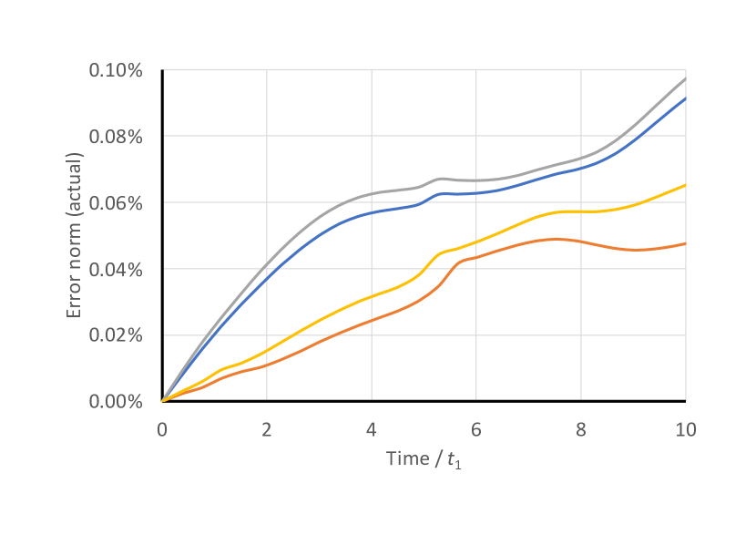
(a) Actual numerical error

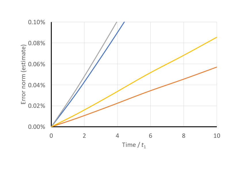
(b) Theoretical error estimate

Figure 1. Error of the mean-field approximation for a family of system-bath models with cubic coupling $W(x,y)=\frac{1}{2}\eta xy^{2}$ as a function of time. The left plot shows the time evolution of the norm of the error for four different variations of the parameter values as given in Table 1. The right plot shows the corresponding upper bound of the error estimate (6.2).

Figure 1 presents the results from the following numerical experiment: We identify a frequency ratio $\varpi_{\rm ref}=1/100$ between bath and system and a coupling parameter $\eta_{\rm ref}=-k_{2}^{0}/(3a_{1}\ell)$ as generating “reference” system-bath dynamics. For this parameter choice, the mean-field approximation, when compared with a numerically converged MCTDH approximation, results in roughly a $0.1\%$ error after $10$ units of the natural harmonic time scale $t_{1}=1/\omega_{1}$ of the system (blue curve), see Figure 1(a). Hence, the Hartree approximation is excellent on the time scale under study. Decreasing the frequency ratio by a factor of four, roughly halves the error (red curve). And, as expected, an increase in the coupling strength also increases the error (grey curve), while decreasing the coupling also decreases the error (yellow curve). The corresponding plot of Figure 1(b) illustrates that the upper bound of the theoretical error estimate correctly captures the initial slope of all four error curves, while slightly over-estimating the actual error as time evolves. A more detailed assessment of the error estimate (6.2), in particular of its long-time behaviour (up to 150 ps), when the mean-field approximation goes up to errors of the order of $1\%$, and a more complete screening of physically relevant parameter régimes are work in progress for a numerical companion paper to the present theoretical study.

7. Conclusion and outlook

We have presented quantitative error bounds for the approximation of quantum dynamical wave functions in product form. For both considered approaches, a brute-force single point collocation and the conventional mean-field Hartree approximation, we have obtained similar error estimates in $L^{2}$-norm (Proposition 3.3, Example 3.5), in $H^{1}$-norm (Proposition 3.9), and for quadratic observables (Proposition 3.11). To our knowledge, such general estimates, that quantify decoupling in terms of flatness properties of the coupling potential, are new. The corresponding analysis for semiclassical subsystems (Proposition 5.5, Proposition 5.8) confirms the more general finding, that error estimates for quadratic observables provide smaller bounds than related norm estimates. The single product analysis, as presented here, provides a well-posed starting point for the investigation of more elaborate approximation methods. If the initial data satisfy

$$\psi(0,x,y)=\psi_{0}(x,y)=\sum_{j=1}^{J}\varphi_{0j}^{x}(x)\varphi_{0j}^{y}(y),$$

then we may invoke the linearity of (1.1) to write $\psi(t,x,y)=\sum_{j=1}^{J}\psi_{j}(t,x,y)$, where each $\psi_{j}$ solves $i{\partial}_{t}\psi_{j}=H\psi_{j}$, with $\psi_{j\mid t=0}=\varphi_{0j}^{x}\otimes\varphi_{0j}^{y}$. We approximate each $\psi_{j}\approx\psi_{j,{\rm app}}$ individually in one of the ways discussed in the present paper and use the triangle inequality for

$$\big{\|}\psi(t)-\sum_{j=1}^{J}\psi_{j,{\rm app}}(t)\big{\|}\leqslant\sum_{j=1}^{J}\|\psi_{j}(t)-\psi_{j,{\rm app}}(t)\|,$$

where the norm can be an $L^{2}$ or an energy norm, for instance. However, working on each $\psi_{j}$ instead of $\psi$ directly, seems to prevent control of the limit $J\to\infty$. Multi-configuration methods therefore use ansatz functions of the form

$$\psi_{\rm app}(t,x,y)=\sum_{j,\ell}a_{j\ell}(t)\,\varphi_{j}^{(x)}(t,x)\,\varphi_{\ell}^{(y)}(t,y),$$

where the families $(\varphi^{(x)}_{j}(t))_{j\geqslant 1}$ and $(\varphi^{(y)}_{\ell}(t))_{\ell\geqslant 1}$ satisfy orthonormality or rank conditions, while gauge constraints lift redundancies for the coefficients $a_{k\ell}(t)\in{\mathbb{C}}$. We view our contributions here as an important first step for a systematic assessment of such multi-configuration approximations in the context of coupled quantum systems. A numerical companion paper, that explores the dynamics of system-bath Hamiltonians with cubic coupling on multiple time-scales with respect to various parameter régimes, is currently in preparation.

Acknowledgements

Adhering to the prevalent convention in mathematics, we chose an alphabetical ordering of authors. We thank Loïc Joubert-Doriol, Gérard Parlant, Yohann Scribano, and Christof Sparber for stimulating discussions in the context of this paper. We acknowledge support from the CNRS 80$|$Prime project AlgDynQua and the visiting professorship program of the I-Site Future.

Appendix A General estimation lemmas

Here we provide the proof of the standard energy estimate, Lemma 4.1.

Proof.

In view of the self-adjointness of $A$, we have

$$\|\psi(t)\|\ \frac{d}{dt}\|\psi(t)\| =\frac{1}{2}\frac{d}{dt}\langle\psi(t),\psi(t)\rangle=\mathrm{Re}\left\langle\psi(t),\frac{1}{ih}(A\psi(t)+\Sigma(t))\right\rangle$$

$$=\frac{1}{h}\mathrm{Im}\langle\psi(t),\Sigma(t)\rangle,$$

and therefore, by the Cauchy–Schwarz inequality, $\frac{d}{dt}\|\psi(t)\|\leqslant\frac{1}{h}\|\Sigma(t)\|$. Integrating in time, we obtain

$$\|\psi(t)\|=\|\psi_{0}\|+\int_{0}^{t}\frac{d}{ds}\|\psi(s)\|ds\leqslant\|\psi_{0}\|+\frac{1}{h}\int_{0}^{t}\|\Sigma(s)\|ds.$$

∎

In the context of observables, refined error estimates will follow from the application of the following lemma.

Lemma A.1.

Let $N\geqslant 1$, $A_{1}$, $A_{2}$, $B$ be self-adjoint on $L^{2}({\mathbb{R}}^{N})$, and $\psi^{(1)},\psi^{(2)}$, solutions to the homogeneous Cauchy problems

$$ih{\partial}_{t}\psi^{(j)}=A_{j}\psi^{(j)}\quad;\quad\psi^{(j)}_{\mid t=0}=\psi_{0},$$

where $\psi_{0}\in L^{2}({\mathbb{R}}^{N})$. Then, for all $t\geqslant 0$

$$\left|\left\langle\psi^{(1)}(t),B\psi^{(1)}(t)\right\rangle-\left\langle\psi^{(2)}(t),B\psi^{(2)}(t)\right\rangle\right|\leqslant\frac{1}{h}\int_{0}^{t}|\rho(s,t)|\,ds,$$

with $\rho(s,t)=\left\langle\psi^{(1)}(s),\left[e^{iA_{2}(t-s)/h}Be^{-iA_{2}(t-s)/h},A_{1}-A_{2}\right]\psi^{(1)}(s)\right\rangle$, where we have denoted by $[\mathcal{A},\mathcal{B}]=\mathcal{AB-BA}$ the standard commutator.

Proof.

We denote the unitary evolution operators by $U_{j}(t)=e^{-iA_{j}t/h}$ and calculate

$$\left\langle\psi^{(1)}(t),B\psi^{(1)}(t)\right\rangle-\left\langle\psi^{(2)}(t),B\psi^{(2)}(t)\right\rangle$$

$$=\left\langle U_{1}(t)\psi_{0},BU_{1}(t)\psi_{0}\right\rangle-\left\langle U_{2}(t)\psi_{0},BU_{2}(t)\psi_{0}\right\rangle$$

$$=\int_{0}^{t}\frac{d}{ds}\left\langle\psi_{0},U_{1}(s)^{*}U_{2}(t-s)^{*}BU_{2}(t-s)U_{1}(s)\psi_{0}\right\rangle ds$$

$$=\frac{1}{ih}\int_{0}^{t}\left\langle\psi_{0},U_{1}(s)^{*}[U_{2}(t-s)^{*}BU_{2}(t-s),A_{1}-A_{2}]U_{1}(s)\psi_{0}\right\rangle ds$$

$$=\frac{1}{ih}\int_{0}^{t}\left\langle\psi^{(1)}(s),[U_{2}(t-s)^{*}BU_{2}(t-s),A_{1}-A_{2}]\psi^{(1)}(s)\right\rangle ds.$$

∎

Appendix B Proof of error estimates: partially flat coupling

In this section, we prove error estimates in $L^{2}$-norm for general potentials $W$ (Remark 3.6), in $H^{1}$-norm (Proposition 3.9), and for quadratic observables (Proposition 3.11).

B.1. Proof of Remark 3.6

To prove the estimates of Example 3.5, recall that we have denoted

$$\eta=\|\left\langle x\right\rangle^{-\sigma_{x}}\langle y\rangle^{-\sigma_{y}}\nabla_{y}W\|_{L^{\infty}}<\infty.$$

The Fundamental Theorem of Calculus yields

$$W(x,y)-W(x,y^{\prime})=(y-y^{\prime})\cdot\int_{0}^{1}\nabla_{y}W\left(y^{\prime}+\theta(y-y^{\prime})\right)d\theta,$$

so we have

$$|W(x,y)-W(x,y^{\prime})| \leqslant|y-y^{\prime}|\left\langle x\right\rangle^{\sigma_{x}}\eta\int_{0}^{1}\left\langle y^{\prime}+\theta(y-y^{\prime})\right\rangle^{\sigma_{y}}d\theta$$

$$\leqslant|y-y^{\prime}|\left\langle x\right\rangle^{\sigma_{x}}\max\left(\left\langle y\right\rangle,\left\langle y^{\prime}\right\rangle\right)^{\sigma_{y}}\eta,$$

and we replace the pointwise estimate of $\delta W$ with

$$|\delta W(x,x^{\prime},y,y^{\prime})|\leqslant|y-y^{\prime}|\left(\left\langle x\right\rangle^{\sigma_{x}}+\left\langle x^{\prime}\right\rangle^{\sigma_{x}}\right)\max\left(\left\langle y\right\rangle,\left\langle y^{\prime}\right\rangle\right)^{\sigma_{y}}\eta.$$

The estimate on $\Sigma_{\phi}$ becomes

$$\|\Sigma_{\phi}\|_{L^{2}}^{2}\leqslant\eta^{2}\int_{{\mathbb{R}}^{n}}\left(\int_{{\mathbb{R}}^{n}}\left(\left\langle x\right\rangle^{\sigma_{x}}+\left\langle x^{\prime}\right\rangle^{\sigma_{x}}\right)|\phi^{x}(t,x^{\prime})|^{2}dx^{\prime}\right)^{2}|\phi^{x}(t,x)|^{2}dx/\|\varphi_{0}^{x}\|^{4}_{L^{2}_{x}}\times$$

$$\times\underbrace{\int_{{\mathbb{R}}^{d}}\left(\int_{{\mathbb{R}}^{d}}|y-y^{\prime}|\max\left(\left\langle y\right\rangle^{\sigma_{y}},\left\langle y^{\prime}\right\rangle^{\sigma_{y}}\right)|\phi^{y}(t,y^{\prime})|^{2}dy^{\prime}\right)^{2}|\phi^{y}(t,y)|^{2}dy/\|\varphi_{0}^{y}\|^{4}_{L^{2}_{y}}}_{=:\epsilon_{y}(t)},$$

and we conclude by resuming the same estimates as above:

$$\int_{{\mathbb{R}}^{n}}\left(\int_{{\mathbb{R}}^{n}}\left(\left\langle x\right\rangle^{\sigma_{x}}+\left\langle x^{\prime}\right\rangle^{\sigma_{x}}\right)|\phi^{x}(t,x^{\prime})|^{2}dx^{\prime}\right)^{2}|\phi^{x}(t,x)|^{2}\frac{dx}{\|\varphi_{0}^{x}\|^{4}_{L^{2}_{x}}}\leqslant 4\|\left\langle x\right\rangle^{\sigma_{x}}\phi^{x}(t)\|_{L^{2}_{x}}^{2},$$

and, in view of the inequality

$$|y-y^{\prime}|\max\left(\left\langle y\right\rangle^{\sigma_{y}},\left\langle y^{\prime}\right\rangle^{\sigma_{y}}\right)\leqslant 2\max\left(\left\langle y\right\rangle^{\sigma_{y}}|y|,\left\langle y^{\prime}\right\rangle^{\sigma_{y}}|y^{\prime}|\right)\leqslant 2\left(\left\langle y\right\rangle^{\sigma_{y}}|y|+\left\langle y^{\prime}\right\rangle^{\sigma_{y}}|y^{\prime}|\right),$$

we find

$$\epsilon_{y}(t)\leqslant 16\|\left\langle y\right\rangle^{\sigma_{y}}|y|\phi^{y}(t)\|_{L^{2}_{y}}^{2}.$$

$\square$

B.2. Proof of Proposition 3.9

To prove error estimates in $H^{1}({\mathbb{R}}^{n+d})$, we differentiate (4.1) in space, and two aspects must be considered: (i) In our framework, the operator $\nabla_{x,y}$ does not commute with $H$. (ii) We must estimate $\nabla_{x,y}\Sigma_{\psi}$ and $\nabla_{x,y}\Sigma_{\phi}$. Indeed, we compute

$$i{\partial}_{t}\nabla_{x}r_{\psi}=H\nabla_{x}r_{\psi}+[\nabla_{x},H]r_{\psi}+\nabla_{x}\Sigma_{\psi},$$

and

$$[\nabla_{x},H]=\nabla_{x}H-H\nabla_{x}=\nabla_{x}V_{1}+\nabla_{x}W.$$

In the typical case where $V_{1}$ is harmonic, $\nabla_{x}V_{1}$ is linear in $x$, and so $xr_{\psi}$ appears as a source term. Note that in the general setting of Assumption 2.1, $|\nabla_{x}V_{1}(x)|\lesssim\left\langle x\right\rangle$.

Remark B.1.

If $\nabla_{x}V_{1}$ and $\nabla_{x}W$ are bounded, then Lemma 4.1 yields

$$\|\nabla_{x}r_{\psi}(t)\|_{L^{2}}\leqslant\int_{0}^{t}\left(C\|r_{\psi}(s)\|_{L^{2}}+\|\nabla_{x}\Sigma_{\psi}(s)\|_{L^{2}}\right)ds.$$

The term $\|r_{\psi}(s)\|_{L^{2}}$ is estimated in Proposition 3.3, and $\|\nabla_{x}\Sigma_{\psi}(s)\|_{L^{2}}$ is estimated below.

Multiplying (4.1) by $x$, we find similarly

$$i{\partial}_{t}(xr_{\psi})=H(xr_{\psi})+[x,H]r_{\psi}+x\Sigma_{\psi}=H(xr_{\psi})+\nabla_{x}r_{\psi}+x\Sigma_{\psi}.$$

Energy estimates provided by Lemma 4.1 applied to the equation for $\nabla_{x}r_{\psi}$ and $xr_{\psi}$ then yield a closed system of estimates:

$$\|\nabla_{x}r_{\psi}(t)\|_{L^{2}}+\|xr_{\psi}(t)\|_{L^{2}} \leqslant\int_{0}^{t}\left(\|(\nabla_{x}V_{1}+\nabla_{x}W)r_{\psi}(s)\|_{L^{2}}+\|\nabla_{x}r_{\psi}(s)\|_{L^{2}}\right)ds$$

$$\quad+\int_{0}^{t}\left(\|\nabla_{x}\Sigma_{\psi}(s)\|_{L^{2}}+\|x\Sigma_{\psi}(s)\|_{L^{2}}\right)ds$$

$$\leqslant C\int_{0}^{t}\left(\|xr_{\psi}(s)\|_{L^{2}}+\|\nabla_{x}r_{\psi}(s)\|_{L^{2}}\right)ds$$

$$\quad+\int_{0}^{t}\left(\|\nabla_{x}\Sigma_{\psi}(s)\|_{L^{2}}+\|x\Sigma_{\psi}(s)\|_{L^{2}}\right)ds,$$

where we have used the estimate $|\nabla_{x}V_{1}+\nabla_{x}W|\leqslant C(1+|x|)$, and the uncertainty principle (uncertainty in $x$, Cauchy-Schwarz in $y$),

$$\|f\|_{L^{2}}^{2}\leqslant\frac{2}{n}\|\nabla_{x}f\|_{L^{2}}\|xf\|_{L^{2}}.$$

The Gronwall Lemma then yields

$$\|\nabla_{x}r_{\psi}(t)\|_{L^{2}}+\|xr_{\psi}(t)\|_{L^{2}}\leqslant\int_{0}^{t}e^{Cs}\left(\|\nabla_{x}\Sigma_{\psi}(s)\|_{L^{2}}+\|x\Sigma_{\psi}(s)\|_{L^{2}}\right)ds,$$

for some $C>0$. We compute

$$\nabla_{x}\Sigma_{\psi}=\left(\nabla_{x}W(x,y)-\nabla_{x}W(x,0)\right)\psi_{\rm app}+\delta W(x,0,y,0)\nabla_{x}\psi_{\rm app}.$$

The first term in controlled by $|y|\|\nabla_{x}\nabla_{y}W\|_{L^{\infty}}|\psi_{\rm app}|$. The second term is controlled like in Section 3.3, by replacing $\psi_{\rm app}$ with $\nabla_{x}\psi_{\rm app}$. We can of course resume the same approach when considering $\nabla_{y}r_{\psi}$, and the analogue of the above first term is now controlled by $|x|\|\nabla_{x}\nabla_{y}W\|_{L^{\infty}}|\psi_{\rm app}|$. Finally, in the case of $r_{\phi}$, computations are similar (we do not keep track of the precise dependence of multiplicative constants here).

B.3. Proof of Proposition 3.11

Proof. We use Lemma A.1 for the operators $H$ and the approximate Hamiltonian $H_{\rm bf}$,

(B.1) $$H_{\rm bf}=H_{x}+H_{y}+W(x,0)+W(0,y)-W(0,0),$$

to obtain

$$|e_{\psi}(t)|\leqslant\int_{0}^{t}|\rho_{\psi}(t,s)|\,ds,$$

where

$$\rho_{\psi}(t,s)=\left\langle\psi_{\rm app}(s),\left[B(t-s),H-H_{\rm bf}\right]\psi_{\rm app}(s)\right\rangle,\quad B(\sigma)=e^{i\sigma H}Be^{-i\sigma H}.$$

By Egorov Theorem, see [42, Theorem 11.1], the operator $B(\sigma)$ is also a pseudodifferential operator, that is, $B(\sigma)={\rm op}(b(\sigma))$ for some function $b(\sigma)$ that satisfies the growth condition 3.5. We have

$$H-H_{\rm bf}=W(x,y)-W(x,0)-W(0,y)+W(0,0)=\delta W(x,0,y,0)=:\delta W(x,y),$$

with the notations of B.1. Then, by the direct estimate of Lemma B.2 below,

$$\|[B(\sigma),\delta W]\psi_{\rm app}(s)\|_{L^{2}}\leqslant C_{b(\sigma)}\left(\|\nabla(\delta W)\psi_{\rm app}(s)\|_{H^{1}}+C_{2}(\delta W)\|\psi_{\rm app}(s)\|_{L^{2}}\right),$$

where $C_{b(\sigma)}>0$ depends on derivative bounds for the function $b(\sigma)$ and

$$C_{2}(\delta W)=\sum_{2\leqslant|\alpha|\leqslant N_{n+d}}\|\partial^{\alpha}\delta W\|_{L^{\infty}}.$$

We therefore obtain

$$|\rho_{\psi}(t,s)|\leqslant\,C_{b(t-s)}\,\Big{(}\|\nabla(\delta W)\psi_{\rm app}(s)\|_{H^{1}}+C_{2}(\delta W)\,\|\psi_{0}\|_{L^{2}}\Big{)}\,\|\psi_{0}\|_{L^{2}}.$$

Using the rectangular $n\times d$ matrix $M(x,y)$ introduced in Remark 3.1, the gradient of $\delta W(x,y)$ can be written as

$$\nabla(\delta W)(x,y)=\left(\begin{array}[]{c}\nabla_{x}W(x,y)-\nabla_{x}W(x,0)\\[4.30554pt] \nabla_{y}W(x,y)-\nabla_{y}W(0,y)\end{array}\right)=\left(\begin{array}[]{c}\int_{0}^{1}M(x,\eta y)y\,d\eta\\[4.30554pt] \int_{0}^{1}\,{}^{t}M(\theta x,y)x\,d\theta\end{array}\right)$$

We estimate the Sobolev norm by

$$\|\nabla(\delta W)\psi_{\rm app}(s)\|_{H^{1}} \leqslant\|\nabla M\|_{L^{\infty}}\left(\|x\psi_{\rm app}(s)\|_{L^{2}}+\|y\psi_{\rm app}(s)\|_{L^{2}}\right)$$

$$\quad+\|M\|_{L^{\infty}}\left(\|\nabla(x\psi_{\rm app}(s))\|_{L^{2}}+\|\nabla(y\psi_{\rm app}(s))\|_{L^{2}}\right),$$

so that integration in time provides

$$|e_{\psi}(t)| \leqslant C_{b}\|\nabla M\|_{L^{\infty}}\|\psi_{0}\|_{L^{2}}\int_{0}^{t}\left(\|x\psi_{\rm app}(s)\|_{L^{2}}+\|y\psi_{\rm app}(s)\|_{L^{2}}\right)ds$$

$$\quad+C_{b}\|M\|_{L^{\infty}}\|\psi_{0}\|_{L^{2}}\int_{0}^{t}\left(\|\nabla(x\psi_{\rm app}(s))\|_{L^{2}}+\|\nabla(y\psi_{\rm app}(s))\|_{L^{2}}\right)ds$$

$$\quad+C_{b}\,C_{2}(\delta W)\,t\,\|\psi_{0}\|_{L^{2}}^{2},$$

where the constant $C_{b}=\max_{\sigma\in[0,t]}C_{b(\sigma)}$ depends on derivatives of $b$. In the mean-field case, the approximate Hamiltonian is time-dependent,

(B.2) $$H_{\rm mf}(t)=H_{x}+H_{y}+\left\langle W\right\rangle_{y}(t)+\left\langle W\right\rangle_{x}(t)-\left\langle W\right\rangle(t).$$

The difference of the Hamiltonians is also a function, which is now time-dependent, $H-H_{\rm mf}(t)=W+\langle W\rangle(t)-\langle W\rangle_{x}(t)-\langle W\rangle_{y}(t)$. However, it is easy to check that a similar estimate can be performed, leading to an analogous conclusion. $\square$

B.4. Commutator estimate

We now explain the commutator estimate used in the previous subsection:

Lemma B.2.

Let $N\geqslant 1$ and $b=b(z,\zeta)$ be a smooth function on ${\mathbb{R}}^{2N}$ satisfying the Hörmander growth condition 3.5. Let $\delta W$ be a smooth function on ${\mathbb{R}}^{N}$ with bounded derivatives. Then, there exist constants $C_{b}>0$ and $M_{N}>0$ such that

$$\|[\mathrm{op}(b),\delta W]\psi\|_{L^{2}}\leqslant C_{b}\,\Big{(}\|\nabla(\delta W)\psi\|_{H^{1}}+\sum_{2\leqslant|\alpha|\leqslant M_{N}}\|\partial^{\alpha}(\delta W)\|_{\infty}\|\psi\|_{L^{2}}\Big{)}$$

for all $\psi\in H^{1}({\mathbb{R}}^{N})$.

Proof.

We explicitly write the commutator as

$$[\mathrm{op}(b),\delta W]\psi(z)=$$

$$(2\pi)^{-N}\int_{{\mathbb{R}}^{2N}}b\left(\frac{z+z^{\prime}}{2},\zeta\right)e^{i\zeta\cdot(z-z^{\prime})}\left(\delta W(z^{\prime})-\delta W(z)\right)\psi(z^{\prime})\,d\zeta dz^{\prime}.$$

We Taylor expand the function $\delta W(z)$ around the point $z^{\prime}$, so that

$$\delta W(z)-\delta W(z^{\prime})=\nabla(\delta W)(z^{\prime})\cdot(z-z^{\prime})+(z-z^{\prime})\cdot\delta R_{2}(z,z^{\prime})(z-z^{\prime})$$

with

$$\delta R_{2}(z,z^{\prime})=\int_{0}^{1}(1-\vartheta)\nabla^{2}(\delta W)(z^{\prime}+\vartheta(z-z^{\prime}))\,d\vartheta.$$

Corresponding to the above decomposition, we write $[\mathrm{op}(b),\delta W]\psi(z)=f_{1}(z)+f_{2}(z)$ and estimate the two summands separately. We observe that $(z-z^{\prime})e^{i\zeta\cdot(z-z^{\prime})}=-i\nabla_{\zeta}e^{i\zeta\cdot(z-z^{\prime})}$ and perform an integration by parts to obtain

$$\int_{{\mathbb{R}}^{2N}}b\left(\frac{z+z^{\prime}}{2},\zeta\right)e^{i\zeta\cdot(z-z^{\prime})}\,\nabla(\delta W)(z^{\prime})\cdot(z-z^{\prime})\,\psi(z^{\prime})\,d\zeta dz^{\prime}$$

$$=i\int_{{\mathbb{R}}^{2N}}\nabla(\delta W)(z^{\prime})\cdot\nabla_{\zeta}b\left(\frac{z+z^{\prime}}{2},\zeta\right)e^{i\zeta\cdot(z-z^{\prime})}\psi(z^{\prime})\,d\zeta dz^{\prime}$$

Therefore,

$$\|f_{1}\|_{L^{2}}\leqslant C_{b}\,\|\nabla(\delta W)\psi\|_{H^{1}},$$

where the constant $C_{b}>0$ depends on derivative bounds of the function $b$. For the remainder term of the above Taylor approximation we write

$$\int_{{\mathbb{R}}^{2N}}b\left(\frac{z+z^{\prime}}{2},\zeta\right)e^{i\zeta\cdot(z-z^{\prime})}\,(z-z^{\prime})\cdot\delta R_{2}(z,z^{\prime})(z-z^{\prime})\,\psi(z^{\prime})\,d\zeta dz^{\prime}$$

$$=\int_{{\mathbb{R}}^{2N}}{\rm tr}\left(\delta R_{2}(z,z^{\prime})\nabla_{\zeta}^{2}b\left(\frac{z+z^{\prime}}{2},\zeta\right)\right)e^{i\zeta\cdot(z-z^{\prime})}\psi(z^{\prime})\,d\zeta dz^{\prime},$$

and obtain that

$$\|f_{2}\|_{L^{2}}\leqslant C_{b}^{\prime}\sum_{2\leqslant|\alpha|\leqslant M_{N}}\|\partial^{\alpha}(\delta W)\|_{\infty}\|\psi\|_{L^{2}},$$

where $C_{b}^{\prime}>0$ depends on derivative bounds of $b$, and $M_{N}>0$ depends on the dimension $N$. ∎

B.5. Proof of energy conservation

Here we provide an elementary ad-hoc proof for energy conservation of the time-dependent Hartree approximation, Lemma 3.14.

Proof.

A first observation is that

$$\left\langle\phi_{\rm app}(t),H_{\rm mf}(t)\phi_{\rm app}(t)\right\rangle=\left\langle\psi_{0},H_{\rm mf}(0)\psi_{0}\right\rangle\quad{\rm for\ all}\ t\geqslant 0.$$

Indeed,

$$\frac{d}{dt}\left\langle\phi_{\rm app}(t),H_{\rm mf}(t)\phi_{\rm app}(t)\right\rangle =\left\langle\phi_{\rm app}(t),\partial_{t}H_{\rm mf}(t)\phi_{\rm app}(t)\right\rangle$$

$$=\left\langle\phi_{\rm app}(t),\partial_{t}W_{\rm app}(t)\phi_{\rm app}(t)\right\rangle$$

with $\displaystyle{W_{\rm app}(t)=\langle W\rangle_{y}(t)+\langle W\rangle_{x}(t)-\left\langle W\right\rangle(t).}$ We deduce

$$\frac{d}{dt}\left\langle\phi_{\rm app}(t),H_{\rm mf}(t)\phi_{\rm app}(t)\right\rangle$$

$$=\int W(x,y)\left({\partial}_{t}|\phi^{x}(t,x)|^{2}\ |\phi^{y}(t,y)|^{2}+|\phi^{x}(t,x)|^{2}\ {\partial}_{t}|\phi^{y}(t,y)|^{2}\right)dxdy$$

$$\quad-\int W(x,y){\partial}_{t}\left(|\phi^{x}(t,x)|^{2}\ |\phi^{y}(t,y)|^{2}\right)dxdy=0,$$

where we have used the self-adjointness of $H_{\rm mf}(t)$ and norm-conservation in the multiplicative components. Secondly, since

$$\left\langle\psi_{0},W_{\rm app}(0)\psi_{0}\right\rangle =\left\langle\psi_{0},\left(\left\langle W\right\rangle_{x}(0)+\left\langle W\right\rangle_{y}(0)-\left\langle W\right\rangle(0)\right)\psi_{0}\right\rangle$$

$$=2\left\langle W\right\rangle(0)-\left\langle W\right\rangle(0)=\left\langle W\right\rangle(0),$$

the approximate energy coincides with the actual energy, and we obtain the aimed for result. ∎

Appendix C Proof of error estimates in the semiclassical régime

Here we present the proofs of the semiclassical estimates given in Proposition 5.5 and Proposition 5.8.

C.1. Error estimates for the wave function

In this section, we prove Proposition 5.5, and comment on the constants $K_{0},K_{1}$, which may be analyzed more explicitly in some cases.

C.1.1. Approximation by partial Taylor expansion

Proof. Section 5.3 defines an approximate solution of the from

$$\psi_{\rm app}^{\varepsilon}(t,x,y)=\varepsilon^{-d/4}e^{(ip(t)\cdot(y-q(t))/\varepsilon+iS(t)/\varepsilon}u_{2}\left(t,\frac{y-q(t)}{\sqrt{\varepsilon}}\right)\psi_{1}^{\varepsilon}(t,x)$$

with

$$i\varepsilon{\partial}_{t}\psi_{1}^{\varepsilon}+\frac{1}{2}\Delta_{x}\psi_{1}^{\varepsilon}=\left(V_{1}(x)+W(x,q)\right)\psi_{1}^{\varepsilon}\quad;\quad\psi^{\varepsilon}_{1\mid t=0}=\varphi_{0}^{x}$$

and

$$i{\partial}_{t}u_{2}+\frac{1}{2}\Delta_{z}u_{2}=\frac{1}{2}\left\langle z,\nabla^{2}V_{2}\left(q\right)z\right\rangle u_{2}\quad;\quad u_{2\mid t=0}=a,$$

$$\dot{q}=p,\,q(0)=q_{0},\quad\dot{p}=-\nabla V_{2}(q),\;p(0)=p_{0},\;\;S(t)=\int_{0}^{t}\left(\frac{|p(s)|^{2}}{2}-V_{2}(q(s))\right)ds.$$

It solves the equation

$$i\varepsilon{\partial}_{t}\psi_{\rm app}^{\varepsilon}+\frac{1}{2}\Delta_{x}\psi_{\rm app}^{\varepsilon}+\frac{\varepsilon^{2}}{2}\Delta_{y}\psi_{\rm app}^{\varepsilon}-V\psi_{\rm app}^{\varepsilon}=\varepsilon^{-d/4}e^{(ip\cdot z/\sqrt{\varepsilon}+iS/\varepsilon}\left(r_{1}^{\varepsilon}+r_{2}^{\varepsilon}\right),$$

where the remainder $r_{1}^{\varepsilon}$ is due to the Taylor expansion in $V_{2}$, and satisfies the pointwise estimate

$$|r_{1}^{\varepsilon}(t,x,z)|\leqslant\frac{1}{6}\times\varepsilon^{3/2}\|\nabla^{3}V_{2}\|_{L^{\infty}_{y}}|\psi_{1}^{\varepsilon}(t,x)|\times|z|^{3}|u_{2}(t,z)|$$

while the remainder $r_{2}^{\varepsilon}$ is due to the Taylor expansion in $W$, and satisfies the pointwise estimate

$$|r_{2}^{\varepsilon}(t,x,z)|\leqslant\sqrt{\varepsilon}\ \|\nabla_{y}W\|_{L^{\infty}}|\psi_{1}^{\varepsilon}(t,x)|\times|z||u_{2}(t,z)|.$$

This implies for the $L^{2}$-norm,

$$\|r_{1}^{\varepsilon}(t)\|_{L^{2}}\leqslant\frac{\varepsilon^{3/2}}{6}\|\nabla^{3}V_{2}\|_{L^{\infty}_{y}}\|\varphi_{0}^{x}\|_{L^{2}_{x}}\||z|^{3}u_{2}(t)\|_{L^{2}_{z}},$$

$$\|r_{2}^{\varepsilon}(t)\|_{L^{2}}\leqslant\sqrt{\varepsilon}\,\|\nabla_{y}W\|_{L^{\infty}}\|\varphi_{0}^{x}\|_{L^{2}_{x}}\|zu_{2}(t)\|_{L^{2}_{z}}.$$

Lemma 4.1 then yields, with now $h=\varepsilon$,

$$\|\psi^{\varepsilon}(t)-\psi_{\rm app}^{\varepsilon}(t)\|_{L^{2}} \leqslant\frac{\sqrt{\varepsilon}}{6}\|\nabla^{3}V_{2}\|_{L^{\infty}_{y}}\|\varphi_{0}^{x}\|_{L^{2}_{x}}\int_{0}^{t}\||z|^{3}u_{2}(s)\|_{L^{2}_{z}}ds$$

$$\quad+\frac{\|\nabla_{y}W\|_{L^{\infty}}}{\sqrt{\varepsilon}}\|\varphi_{0}^{x}\|_{L^{2}_{x}}\int_{0}^{t}\||z|u_{2}(s)\|_{L^{2}_{z}}ds.$$

According to the signature of $\nabla^{2}V_{2}(q(t))$, the quantities $\||z|^{3}u_{2}(s)\|_{L^{2}_{z}}$ and $\||z|u_{2}(s)\|_{L^{2}_{z}}$ may be bounded uniformly in $s\geqslant 0$ or not. For instance, they are bounded if $\nabla^{2}V_{2}$ is uniformly positive definite, or at least uniformly positive definite along the trajectory $q$. On the other hand, we always have an exponential bound, even if it may not be sharp,

$$\||z|^{3}u_{2}(s)\|_{L^{2}_{z}}+\||z|u_{2}(s)\|_{L^{2}_{z}}\leqslant C_{0}e^{C_{1}s},$$

for some constants $C_{0},C_{1}>0$. This control is sharp in the case where $\nabla^{2}V_{2}$ is uniformly negative definite. See e.g. [8, Lemma 10.4] for a proof of the exponential control, and [8, Section 10.5] for a discussion on its optimality. In particular, for bounded time intervals, the (relative) error is small if $\|\nabla_{y}W\|_{L^{\infty}}\ll\sqrt{\varepsilon}\ll 1$. $\square$

Remark C.1.

If $\nabla_{y}W$ is not bounded, e.g. $\nabla_{y}W(x,y)=\eta\left\langle x\right\rangle^{\gamma}$, then we can replace the previous error estimate with

$$\|\psi^{\varepsilon}(t)-\psi^{\varepsilon}_{\rm app}(t)\|_{L^{2}} \leqslant\frac{\sqrt{\varepsilon}}{6}\|\nabla^{3}V_{2}\|_{L^{\infty}_{y}}\|\varphi_{0}^{x}\|_{L^{2}_{x}}\int_{0}^{t}\||z|^{3}u_{2}(s)\|_{L^{2}_{z}}ds$$

$$\quad+\frac{\eta}{\sqrt{\varepsilon}}\int_{0}^{t}\|\left\langle x\right\rangle^{\gamma}\psi_{1}^{\varepsilon}(s)\|_{L^{2}_{x}}\||z|u_{2}(s)\|_{L^{2}_{z}}ds.$$

In other words, the cause for the unboundedness of $\nabla_{y}W$ is transferred to a weight for $\psi_{1}^{\varepsilon}$. Similarly, if $\nabla_{y}W$ is unbounded in $y$, we may change the weight in the terms $\||z|^{k}u_{2}\|_{L^{2}_{z}}$, after substituting $y$ with $q+z\sqrt{\varepsilon}$.

C.1.2. Approximation by partial averaging

Proof.

The semiclassical approximation obtained by partial averaging reads:

$$\psi_{\rm app}^{\varepsilon}(t,x,y)=\varepsilon^{-d/4}e^{ip(t)\cdot(y-q(t))/\varepsilon+iS(t)/\varepsilon}u_{2}\left(t,\frac{y-q(t)}{\sqrt{\varepsilon}}\right)\psi_{1}^{\varepsilon}(t,x)$$

with

$$i\varepsilon{\partial}_{t}\psi_{1}^{\varepsilon}+\frac{1}{2}\Delta_{x}\psi_{1}^{\varepsilon}=\left(V_{1}(x)+\left\langle W(x,\cdot)\right\rangle_{y}(t)\right)\psi_{1}^{\varepsilon}\quad;\quad\psi_{1\mid t=0}^{\varepsilon}=\varphi_{0}^{x}$$

and

$$i{\partial}_{t}u_{2}+\frac{1}{2}\Delta_{z}u_{2}=\frac{1}{2}\ z\cdot\left\langle\nabla^{2}V_{2}\right\rangle_{y}\!(t)z\ u_{2}\quad;\quad u_{2\mid t=0}=a,$$

$$\dot{q}=p,\quad q(0)=q_{0},\quad\dot{p}=-\langle\nabla V_{2}\rangle_{y}(t),\quad p(0)=p_{0},\;\;\dot{S}(t)=\frac{|p(t)|^{2}}{2}-\langle V_{2}\rangle_{y}(t).$$

To estimate the size of $\tilde{r}_{1}$ and $\tilde{r}_{2}$ introduced in Section 5.4, we might argue again via Taylor expansion. Indeed,

$$\|a\|_{L^{2}}^{2}\left\langle V_{2}\right\rangle_{y} =\int V_{2}(q(t)+\sqrt{\varepsilon}z)\ |u_{2}(t,z)|^{2}dz$$

$$=V_{2}(q(t))+\sqrt{\varepsilon}\,\nabla V_{2}(q(t))\cdot\int z|u_{2}(t,z)|^{2}dz+r_{3}^{\varepsilon}(t),$$

where

$$|r_{3}^{\varepsilon}(t)|\leqslant\frac{\varepsilon}{2}\|\nabla^{2}V_{2}\|_{L^{\infty}}\left\||z|u_{2}(t,z)\right\|^{2}_{L^{2}_{z}}.$$

Hence, we have for all averages $f=V_{2},\nabla V_{2},\nabla^{2}V_{2},W(x,\cdot)$ that

$$\left\langle f\right\rangle_{y}(t)=f\left(q(t)\right)+\mathcal{O}(\sqrt{\varepsilon}),$$

where the error constant depends on moments of $|u_{2}|^{2}$. In particular, if $u_{2}(0)$ is Gaussian, the odd moments of $|u_{2}(t,z)|^{2}$ vanish, and the above estimate improves to $\mathcal{O}(\varepsilon)$. Hence, the $L^{2}$-norm of $\tilde{r}_{1}$ is $\mathcal{O}(\sqrt{\varepsilon})$ close to the $L^{2}$-norm of $r_{1}$, and the $L^{2}$-norm of $\tilde{r}_{2}$ is $\mathcal{O}(\eta\sqrt{\varepsilon})$, $\eta=\|\nabla_{y}W\|_{L^{\infty}}$, close to the $L^{2}$-norm of $r_{2}$ (with each time an extra $\sqrt{\varepsilon}$ gain in the above mentioned Gaussian case). In particular, the order of magnitude for the difference between exact and approximate solution is the same as in the previous subsection, only multiplicative constants are affected. We emphasize that the constants $C_{0}$ and $C_{1}$ from the previous subsection are in general delicate to assess. On the other hand, in specific cases (typically when $u_{2}$ is Gaussian and $\nabla^{2}V_{2}$ is known), they can be computed rather explicitly. ∎

C.2. Error estimates for quadratic observables

The proof of Proposition 5.8 is discussed in the next two sections.

C.2.1. Approximation by Taylor expansion

Proof.

Taylor expansion yields a time-dependent Hamiltonian $H_{\rm app}^{\varepsilon}=H^{\varepsilon}_{\rm te}$ with

$$H^{\varepsilon}_{\rm te} :=-\frac{1}{2}\Delta_{x}-\frac{\varepsilon^{2}}{2}\Delta_{y}+V_{1}(x)+W(x,q)+V_{2}(q)+(y-q)\cdot\nabla V_{2}(q)$$

$$\quad+\frac{1}{2}\left\langle y-q,\nabla^{2}V_{2}(q)(y-q)\right\rangle,$$

where $q=q(t)$. In particular, the difference $H^{\varepsilon}-H^{\varepsilon}_{\rm te}$ is a function,

$$H^{\varepsilon}-H^{\varepsilon}_{\rm te} =W(x,y)-W(x,q)+V_{2}(y)-V_{2}(q)-(y-q)\cdot\nabla V_{2}(q)$$

$$\quad-\frac{1}{2}\left\langle y-q,\nabla^{2}V_{2}(q)(y-q)\right\rangle=:\delta W(t,x,y).$$

In view of Lemma A.1, if $B={\rm op}_{\varepsilon}(b)$ with $b\in C^{\infty}_{c}({\mathbb{R}}^{2d})$, it yields (a posteriori estimate)

$$\left|\left\langle\psi^{\varepsilon}(t),B\psi^{\varepsilon}(t)\right\rangle-\left\langle\psi^{\varepsilon}_{\rm app}(t),B\psi^{\varepsilon}_{\rm app}(t)\right\rangle\right|\leqslant\frac{1}{\varepsilon}\int_{0}^{t}|\rho^{\varepsilon}(t,x)|ds,$$

where

$$\rho^{\varepsilon}(t,s)=\left\langle\psi^{\varepsilon}_{\rm app}(s),[B(t-s),\delta W(s)]\psi^{\varepsilon}_{\rm app}(s)\right\rangle,\quad B(\sigma)=e^{i\sigma H/\varepsilon}Be^{-i\sigma H/\varepsilon}.$$

By Egorov Theorem [42, Theorem 11.1], $B(\sigma)=\varepsilon\,\mathrm{op}_{\varepsilon}(b(\sigma))$ for a function $b(\sigma)\in C^{\infty}_{c}({\mathbb{R}}^{d})$. Therefore, by semiclassical calculus,

$$\frac{1}{i\varepsilon}[B(t-s),\delta W(s)]=\mathrm{op}_{\varepsilon}\left(\{b(t-s),\delta W(s)\}\right)+\varepsilon^{2}\mathrm{op}_{\varepsilon}\left(r^{\varepsilon}(s,t)\right),$$

where $\|\mathrm{op}_{\varepsilon}(r^{\varepsilon}(s,t))\|_{\mathcal{L}(L^{2})}$ is bounded uniformly in $\varepsilon$, whence the estimate of Proposition 5.8. ∎

C.2.2. Approximation by partial averaging

Proof.

The time-dependent Hamiltonian is ${H}_{\rm app}^{\varepsilon}={H}_{\rm pa}^{\varepsilon}$ with

$${H}_{\rm pa}^{\varepsilon} =-\frac{1}{2}\Delta_{x}-\frac{\varepsilon^{2}}{2}\Delta_{y}+V_{1}(x)+\langle W(x,\cdot)\rangle_{y}+\langle V_{2}\rangle_{y}(t)+(y-q)\cdot\langle\nabla V_{2}\rangle_{y}(t)$$

$$\quad+\frac{1}{2}(y-q)\cdot\langle\nabla^{2}V_{2}\rangle_{y}(t)(y-q),$$

where $q=q(t)$. In particular, as in the preceding case, the difference $H^{\varepsilon}-{H}_{\rm pa}^{\varepsilon}$ is a time-dependent function

$$H^{\varepsilon}-{H}^{\varepsilon}_{\rm pa} =W(x,y)-\langle W(x,\cdot)\rangle_{y}+V_{2}(y)-\langle V_{2}\rangle_{y}(t)$$

$$\quad-(y-q)\cdot\langle\nabla V_{2}\rangle_{y}(t)-\frac{1}{2}(y-q)\cdot\langle\nabla^{2}V_{2}\rangle_{y}(t)(y-q)=:\widetilde{\delta W}(t,x,y),$$

and the arguments developed above also apply. ∎

C.3. Time-adiabatic approximation

The evolution equations for the quantum part of the system, equations (5.8) and (5.11), can be written as an adiabatic problem:

$$i\varepsilon\partial_{t}\psi_{1}^{\varepsilon}(t)=\mathfrak{h}(t)\psi_{1}^{\varepsilon}(t),\;\;\psi_{1}^{\varepsilon}(0)=\varphi_{0}^{x},$$

where $\mathfrak{h}(t)$ is one of the time-dependent self-adjoint operators on $L^{2}({\mathbb{R}}^{n})$

$$\mathfrak{h}_{\rm te}(t)=-\frac{1}{2}\Delta+V_{1}(x)+W(x,q(t))\;\;\mbox{and}\;\;\mathfrak{h}_{\rm pa}(t)=-\frac{1}{2}\Delta+V_{1}(x)+\langle W(x,.)\rangle_{y}(t).$$

We assume here that $\mathfrak{h}(t)$ has a compact resolvent and thus, that its spectrum consists in a sequence of time-dependent eigenvalues

$${\Lambda}_{1}(t)\leqslant{\Lambda}_{2}(t)\leqslant\cdots\leqslant{\Lambda}_{k}(t)\mathop{\longrightarrow}\limits_{k\rightarrow+\infty}\infty.$$

We also assume that some eigenvalue ${\Lambda}_{j}(t)$ is separated from the remainder of the spectrum for all $t\in{\mathbb{R}}$ and that the initial datum $\varphi_{0}^{x}$ is in the eigenspace of $\mathfrak{h}(0)$ for the eigenvalue ${\Lambda}_{j}(0)$:

(C.1) $$\mathfrak{h}(0)\varphi_{0}^{x}={\Lambda}_{j}(0)\varphi_{0}^{x}.$$

Then adiabatic theory as developed by Kato [22] states that $\psi_{1}(t)$ stays in the eigenspace of ${\Lambda}_{j}(t)$ on finite time, up to a phase.

Proposition C.2 (Kato [22]).

Assume we have (C.1) and that ${\Lambda}_{j}(0)$ is a simple eigenvalue of $\mathfrak{h}(0)$ such that there exists $\delta_{0}>0$ for which

$$d\left(\{{\Lambda}_{j}(t)\},{\rm Sp}(\mathfrak{h}(t))\setminus\{{\Lambda}_{j}(t)\}\right)\geq\delta_{0}.$$

Denote by $\Phi_{j}^{x}(t)$ a family of normalized eigenvectors of $\mathfrak{h}(t)$ such that

$$\Phi_{j}^{x}(0)=\varphi_{0}^{x},\quad\left\langle\Phi^{x}_{j}(t),\partial_{t}\Phi_{j}^{x}(t)\right\rangle=0.$$

Then, for all $T>0$, there exists a constant $C_{T}>0$ such that

$$\left\|\psi_{1}^{\varepsilon}(t)-e^{-\frac{i}{\varepsilon}\int_{0}^{t}{\Lambda}_{j}(s)ds}\Phi^{x}_{j}(t,x)\right\|_{L^{2}_{x}}\leqslant C_{T}\varepsilon.$$

In contrast to the Born-Oppenheimer point of view recalled in Remark 5.4, we obtain the following time-adiabatic extension for our wave-packet approximation:

Corollary C.3.

In the setting of Proposition 5.5 and Proposition C.2, we obtain the following approximate solution

$$\psi^{\varepsilon}_{\rm app}(t,x,y)=e^{-\frac{i}{\varepsilon}\int_{0}^{t}{\Lambda}_{j}(s)ds+\frac{i}{\varepsilon}S(t)+\frac{i}{\varepsilon}p(t)\cdot(y-q(t))}\Phi^{x}_{j}(t,x)u_{2}\left(t,\frac{y-q(t)}{\sqrt{\varepsilon}}\right).$$

Appendix D Material for the numerical simulations

All numerical calculations for the Section 6 were run with the QUANTICS (Version 2.0) suite of programs for molecular quantum dynamics simulations [G. A. Worth, K. Giri, G. W. Richings, I. Burghardt, M. H. Beck, A. Jäckle, and H.-D. Meyer. The QUANTICS Package, Version 2.0, (2020), University College London, London, U.K.].

D.1. TDH and MCTDH calculations

For each set of parameters we compared mean-field (TDH) calculations (one single-particle function per mode) to converged Multiconfiguration Time-Dependent Hartree (MCTDH) calculations (three single-particle functions per mode, i.e., nine configurations). The latter were compared to numerically “exact” standard propagations on a two-dimensional grid, showing virtually no difference. In all cases, we chose for the primitive basis set a direct product of Gauss–Hermite functions ($128\times 1024$) associated to the local harmonic approximation of the potential energy centered at $(x,y)=(0,0)$. We used default integrator schemes for both TDH and MCTDH: norm and energy preservation were dutifully checked. The initial datum of each situation was chosen as a quasi-coherent state corresponding to the local harmonic ground state (centered at $(x,y)=(0,0)$, with no extra momentum, and with natural widths $1/\sqrt{2}$ in natural units).

D.2. Model set-up

Calculations were run with dimensioned parameters and variables, all given numerically in terms of atomic units with realistic values chosen to be representative of what can be encountered in a typical organic molecule. The only quantity left with a dimension is time. The time scale used in both Figures is the natural time for the system coordinate $x$, namely $t_{1}=1/\omega_{1}=\hbar/E_{1}$, which within our settings is equal to $109.74$ a.u. ($2.6544$ fs). We used a unit local curvature at the origin in natural units and a double-well width $\ell=4$. In atomic units, where we chose $a_{1}=0.24536$ bohr, we have a dimensioned $a_{1}\cdot\ell=0.98142$ bohr.

D.3. The reference model, blue curves

Masses::

$\mu_{1}=1$ amu = 1822.9 m_e, $\mu_{2}=16$ amu = 29166 m_e, $\varepsilon=\sqrt{\mu_{1}/\mu_{2}}=1/4$

Energies/frequencies::

$\omega_{1}=2000$ cm${}^{-1}=0.0091127$ hartree, $\omega_{2}=20$ cm${}^{-1}=0.000091127$ hartree , $\varpi=\omega_{2}/\omega_{1}=1/100$

Natural scales for $x$::

$a_{1}=0.24536$ bohr (length), $E_{1}=0.0091127$ hartree (energy), $t_{1}=109.74\hbar$ hartree${}^{-1}=2.6544$ fs (time)

Double-well width::

$\ell=4$, i.e., $L=4a_{1}=0.98142$ bohr

Width for the initial datum::

$\sigma_{1}=a_{1}/\sqrt{2}=0.17349$ bohr, $\sigma_{2}=a_{2}/\sqrt{2}=0.43373$ bohr, where $a_{2}=\epsilon/\sqrt{\varpi}a_{1}=10/4a_{1}$

Coupling constant:

$\eta=-k_{2}/(3L)=-0.000082261$ a.u., where $k_{2}=\mu_{2}\,\omega_{2}^{2}$

D.4. Variations of the blue model

Red curves::

softer bath, but same coupling relation $\eta=-k_{2}/(3L)$
$\omega_{2}=0.000022782$ a.u. such that $\varpi=1/400$; $\sigma_{2}$ = 0.86747 bohr, $\eta=-0.0000051413$ a.u. both depend on $\omega_{2}$

Gray curves::

same bath but stronger coupling $\eta=-3/8\,k_{2}/L$
$\varpi,\omega_{2},\sigma_{2}$ unchanged against original model, $\eta=-0.000092543$ a.u.

Yellow curves::

same bath but weaker coupling $\eta=-k_{2}/(4L)$
$\varpi,\omega_{2},\sigma_{2}$ unchanged against original model, $\eta=-0.000030848$ a.u.

References

- [1] S. Alinhac and P. Gérard. Pseudo-differential operators and the Nash-Moser theorem, volume 82 of Graduate Studies in Mathematics. American Mathematical Society, Providence, RI, 2007. Translated from the 1991 French original by Stephen S. Wilson.
- [2] G. D. Billing. On the use of Ehrenfest’s theorem in molecular scattering. Chem. Phys. Lett., 100:535, 1983.
- [3] H. Breuer and F. Petruccione. The theory of open quantum systems. Oxford University Press, Oxford, 2002.
- [4] P. R. Bunker and P. Jensen. Molecular symmetry and spectroscopy. NRC Research Press, Ottawa, 2006.
- [5] I. Burghardt and et al. Approaches to the approximate treatment of complex molecular systems by the multiconfiguration time-dependent hartree method. J. Chem. Phys., 111:2927, 1999.
- [6] I. Burghardt and G. Parlant. On the dynamics of coupled Bohmian and phase-space variables: A new hybrid quantum-classical approach. J. Chem. Phys., 120:3055, 2004.
- [7] E. Cancès and C. Le Bris. On the time-dependent Hartree-Fock equations coupled with a classical nuclear dynamics. Math. Models Methods Appl. Sci., 9(7):963–990, 1999.
- [8] R. Carles. Semi-classical analysis for nonlinear Schrödinger equations: WKB analysis, focal points, coherent states. World Scientific Publishing Co. Pte. Ltd., Hackensack, NJ, 2nd edition, xiv-352 p. 2021.
- [9] R. Carles and C. Fermanian Kammerer. Nonlinear coherent states and Ehrenfest time for Schrödinger equations. Commun. Math. Phys., 301(2):443–472, 2011.
- [10] J. Caro and L. Salcedo. Impediments to mixing classical and quantum dynamics. Phys. Rev. A, 60:842, 1999.
- [11] R. D. Coalson and M. Karplus. Multidimensional variational gaussian wave packet dynamics with application to photodissociation spectroscopy. The Journal of Chemical Physics, 93(6):3919–3930, 1990.
- [12] M. Combescure and D. Robert. Coherent states and applications in mathematical physics. Theoretical and Mathematical Physics. Springer, Dordrecht, 2012.
- [13] J. B. Delos, W. R. Thorson, and S. K. Knudson. Semiclassical theory of inelastic collisions. I. Classical picture and semiclassical formulation. Phys. Rev. A, 6:709, 1972.
- [14] P. A. M. Dirac. Note on exchange phenomena in the Thomas atom. Proc. Cambridge Philos. Soc., 26:376, 1930.
- [15] F. Gatti, B. Lasorne, H.-D. Meyer, and A. Nauts. Applications of Quantum Dynamics in Chemistry. Lectures Notes in Chemistry. Springer International Publishing, 2017.
- [16] R. B. Gerber, V. Buch, and M. A. Ratner. Time-dependent self-consistent field approximation for intramolecular energy transfer: I. Formulation and application to dissociation of van der Waals molecules. J. Chem. Phys., 77:3022, 1982.
- [17] E. Gindensperger, C. Meier, and J. A. Beswick. Mixing quantum and classical dynamics using Bohmian trajectories. J. Chem. Phys., 113:9369, 2000.
- [18] M. Gruebele. Quantum dynamics and control of vibrational dephasing. J. Phys.: Condens. Matter, 16:R1057, 2004.
- [19] B. Jäger, R. Hellmann, E. Bich, and E. Vogel. State-of-the-art ab initio potential energy curve for the krypton atom pair and thermophysical properties of dilute krypton gas. J. Chem. Phys., 144:114304, 2016.
- [20] S. Jin, C. Sparber, and Z. Zhou. On the classical limit of a time-dependent self-consistent field system: analysis and computation. Kinet. Relat. Models, 10(1):263–298, 2017.
- [21] R. Kapral and G. Ciccotti. Mixed quantum-classical dynamics. J. Chem. Phys., 110:8919, 1999.
- [22] T. Kato. On the adiabatic theorem of quantum mechanics,. J. Phys. Soc. Japan, 5:435–439, 1950.
- [23] C. Lasser and C. Lubich. Computing quantum dynamics in the semiclassical regime. Acta Numer., 29:229–401, 2020.
- [24] A. M. Levine, M. Shapiro, and E. Pollak. Hamiltonian theory for vibrational dephasing rates of small molecules in liquids. J. Chem. Phys., 88:1959, 1988.
- [25] C. Lubich. On variational approximations in quantum molecular dynamics. Math. Comp., 74(250):765–779, 2005.
- [26] C. Lubich. From quantum to classical molecular dynamics: reduced models and numerical analysis. Zurich Lectures in Advanced Mathematics. European Mathematical Society (EMS), Zürich, 2008.
- [27] C. C. Martens and J.-Y. Fang. Semiclassical-limit molecular dynamics on multiple electronic surfaces. J. Chem. Phys., 106:4918, 1994.
- [28] A. Martinez and V. Sordoni. Twisted pseudodifferential calculus and application to the quantum evolution of molecules. Mem. Amer. Math. Soc., 200(936):vi+82, 2009.
- [29] M. Nest and H.-D. Meyer. Dissipative quantum dynamics of anharmonic oscillators with the multiconfiguration time-dependent hartree method. J. Chem. Phys., 119, 24, 2003.
- [30] M. Reed and B. Simon. Methods of modern mathematical physics. II. Fourier analysis, self-adjointness. Academic Press [Harcourt Brace Jovanovich Publishers], New York, 1975.
- [31] S. Römer and I. Burghardt. Towards a variational formulation of mixed quantum-classical molecular dynamics. Molecular Physics, 111(22-23):3618–3624, 2013.
- [32] L. L. Salcedo. Statistical consistency of quantum-classical hybrids. Phys. Rev. A, 85:022127, 2012.
- [33] F. Schroeder and A. W. Chin. Simulating open quantum dynamics with time-dependent variational matrix product states: towards microscopic correlation of environment dynamics and reduced system evolution. Phys. Rev. B, 93:075105, 2016.
- [34] A. Strathearn and et al. Efficient non-markovian quantum dynamics using time-evolving matrix product operators,. Nature Comm., 9:3322, 2018.
- [35] W. Struyve. Semi-classical approximations based on Bohmian mechanics. Int. J. Mod. Phys. A, 35:2050070, 2020.
- [36] D. Tamascelli and et al. Efficient simulation of finite-temperature open quantum systems. Phys. Rev. Lett., 123:090402, 2019.
- [37] D. R. Terno. Inconsistency of quantum-classical dynamics, and what it implies. Found. Phys., 36:102, 2006.
- [38] S. Teufel. Adiabatic perturbation theory in quantum dynamics, volume 1821 of Lecture Notes in Mathematics. Springer-Verlag, Berlin, 2003.
- [39] H. Wang. Multilayer multiconfiguration time-dependent hartree theory. J. Phys. Chem. A, 119:7951, 2015.
- [40] H. Wei, R. J. Le Roy, R. Wheatley, and W. J. Meath. A reliable new three-dimensional potential energy surface for H2-Kr. J. Chem. Phys., 122:084321, 2005.
- [41] U. Weiss. Quantum dissipative systems, 4th Ed. World Scientific, Singapore, 2012.
- [42] M. Zworski. Semiclassical analysis, volume 138 of Graduate Studies in Mathematics. American Mathematical Society, Providence, RI, 2012.