Limiting laws and consistent estimation criteria for fixed and diverging number of spiked eigenvalues

Abstract

In this paper, we study limiting laws and consistent estimation criteria for the extreme eigenvalues in a spiked covariance model of dimension $p$ with the number of spikes $k$. Allowing both $p$ and $k$ to diverge, we derive limiting distributions of the spiked sample eigenvalues using random matrix theory techniques. Notably, our results are established under a general spiked covariance model, where the bulk eigenvalues are allowed to differ, and the spiked eigenvalues need not be uniformly upper bounded or tending to infinity, as have been assumed in the existing literature. Based on the above derived results, we formulate generalized estimation criteria that can consistently estimate $k$, while $k$ can be fixed or grow at an order of $k=o(n^{1/3})$. Our results are established under both Gaussian distributions and general distributions with finite fourth moments, with different growth rate conditions on $k$. The effectiveness of the proposed estimation criteria is illustrated through simulation studies and applications to two real-world data sets.

Keywords: AIC; BIC; principal component analysis; random matrix theory; spiked covariance model.

1 Introduction

Principal component analysis (PCA) has been widely used for a range of purposes including dimension reduction, data visualization, and downstream supervised or unsupervised learning (Abdi and Williams, 2010). In PCA, the leading eigenvalues and eigenvectors of the population covariance matrix are estimated using their empirical counterparts. Hence, it is important to understand properties of the sample covariance matrix, and to investigate how to determine the number of significant components using the sample covariance matrix.

Consider a sample of size $n$ denoted as ${\mathbf{x}}_{1},\ldots,{\mathbf{x}}_{n}$ from a $p$-dimensional multivariate distribution with mean ${\mathbf{0}}$ and covariance ${\mathbf{\Sigma}}_{p\times p}$. Let $\lambda_{1}\geq\cdots\geq\lambda_{p}$ denote the eigenvalues of ${\mathbf{\Sigma}}$. In our work, we focus on the setting with $\lambda_{1}\geq\cdots\geq\lambda_{k}>\lambda_{k+1}\geq\cdots\geq\lambda_{p}$, typically referred to as the general spiked covariance model (Ke et al., 2023). The number, $k$, is referred to as the number of signals or the number of spikes. This model is a generalization of the standard spiked covariance model (Johnstone, 2001) that assumes $\lambda_{1}\geq\cdots\geq\lambda_{k}>\lambda_{k+1}=\cdots=\lambda_{p}$. Let ${\mathbf{S}}_{n}=\sum_{i=1}^{n}{\mathbf{x}}_{i}{\mathbf{x}}_{i}^{\top}/n$ be the sample covariance matrix and denote its eigenvalues by $d_{1}\geq\cdots\geq d_{p}$. In this work, we study limiting laws of $d_{1},\ldots,d_{k}$, referred to as spiked sample eigenvalues, and derive consistent criteria for estimating the number of spikes, $k$, in both fixed and diverging $p$ regimes. The three main focuses of this work are detailed as below.

As a first focus of this paper, we aim to study the limiting laws of $d_{1},\ldots,d_{k}$ when $p\rightarrow\infty$. Under this regime, many efforts have been made to understand the behaviors of the eigenvalues and eigenvectors of ${\mathbf{S}}_{n}$; see, for example, Jonsson (1982), Johansson (1998), Bai and Silverstein (2004), Paul (2007), Nadakuditi and Edelman (2012), Ma (2012), Onatski et al. (2013), Wang and Yao (2013), Wang et al. (2014), Passemier et al. (2015), Wang and Fan (2017), Bai et al. (2018), Cai et al. (2020), Li et al. (2020), Jiang and Bai (2021) and Zhang et al. (2022). Assuming that $n,p\to\infty$, $p/n\rightarrow c>0$, we establish the limit of the spiked sample eigenvalue $d_{i}$ for $1\leq i\leq k$ under regularity conditions. Notably, our result allows $k$ to diverge at the rate of $o(n^{1/3})$ for Gaussian distributions and $o(n^{1/4})$ for general distributions with finite fourth moments. This is improved over what has been established in the literature, such as $k=o(n^{1/6})$ in Cai et al. (2020). Moreover, we show that $d_{i}$, $1\leq i\leq k$, is $\sqrt{n/k}$-consistent and demonstrate its asymptotic normality. An important improvement of our work over most known results in the literature is that our results hold even when the number of the spikes $k$ diverges. Furthermore, our results allow for general spiked eigenvalues $\lambda_{1},\ldots,\lambda_{k}$, as we do not require them to be uniformly upper bounded or tending to infinity, and for general bulk eigenvalues $\lambda_{k+1},\ldots,\lambda_{p}$ that may differ from each other.

As a second focus of this paper, we aim to investigate consistent information criteria for estimating $k$ under a fixed $p$. Under this setting, commonly considered criteria for estimating the number of spikes $k$ include AIC (Wax and Kailath, 1985; Zhao et al., 1986), with a penalty term $v(k,p)$, and BIC (Wax and Kailath, 1985; Zhao et al., 1986), with a penalty term $v(k,p)\log n/2$, where $v(k,p)$ denotes the number of free parameters under $k$. An important work by Zhao et al. (1986) showed that any penalty term $C_{n}v(k,p)$ may lead to an asymptotically consistent estimator, as long as $C_{n}/\log\log n\to\infty$ and $C_{n}/n\to 0$. Under general distributions with finite fourth moments and a standard spiked covariance model, we give a non-asymptotic result and show that consistency can be ensured as long as $C_{n}\to\infty$ and $C_{n}/n\to 0$, which much relaxes the condition in Zhao et al. (1986) and broadens the class of consistent estimation criteria. For example, based on our result, both $C_{n}=\log\log n$ and $C_{n}=(\log\log n)^{1/2}$ lead to consistent estimation criteria. As discussed in Kritchman and Nadler (2009) and Nadler (2010), although BIC is asymptotically consistent, the penalty term with $C_{n}=\log n/2$ can be too large in finite sample and lead to underestimation, especially when the signal to noise ratio (SNR) is low. Hence, our result offers theoretical guarantee for weaker penalty terms compared to BIC.

As a third focus of this paper, we aim to investigate consistent information criteria for $k$ when $p\rightarrow\infty$. In this regime, important progresses have been made recently on estimating the number of spikes in PCA or the number of factors in factor analysis, using methods such as information criterion (Bai and Ng, 2002; Bai et al., 2018; Chen and Li, 2022), identifying eigengap (Onatski, 2009; Passemier and Yao, 2014; Cai et al., 2020), hypothesis testing (Ke, 2016; Bao et al., 2022) and eigenvalue thresholding (Buja and Eyuboglu, 1992; Saccenti and Timmerman, 2017; Dobriban and Owen, 2019; Dobriban, 2020; Jiang and Bai, 2021; Fan et al., 2022; Ke et al., 2023). Most existing works focused on a fixed $k$ as $n,p\rightarrow\infty$. Ke (2016) allowed a divergent $k$ but only for testing $H_{0}:{\mathbf{\Sigma}}={\mathbf{I}}$ against a spiked covariance matrix as the alternative. Some works also required the spiked eigenvalues $\lambda_{1},\ldots,\lambda_{k}$ to diverge (Bai and Ng, 2002; Cai et al., 2020) or be uniformly upper bounded (Bai et al., 2018; Jiang and Bai, 2021), while some required the population eigenvectors to satisfy certain forms of “delocalization” conditions (Dobriban and Owen, 2019; Dobriban, 2020) or sparsity conditions (Fan et al., 2022).

In our work, we propose consistent generalized information criteria that allow for general spiked eigenvalues, in that they need not be divergent or uniformly upper bounded, a fixed $k$ or $k=o(n^{1/3})$, and without requiring delocalization or sparsity conditions on the eigenvectors. Specifically, under the standard spiked covariance model with general distributions with finite fourth moments, we propose a generalized information criterion (GIC) that includes AIC and BIC as special cases, and is shown to achieve consistency under more general conditions compared to those established in Bai et al. (2018) for AIC and BIC. Furthermore, under the general spiked covariance model, motivated by the adjusted eigenvalue thresholding procedure in Fan et al. (2022), we propose an adjusted GIC that is consistent under general distributions with finite moments of order greater than 4. In Section 4, we compare our proposed estimation criteria with many existing methods including those mentioned above, and demonstrate their efficacy.

Main contributions. To summarize, the main contributions of our work are threefold. Firstly, for diverging $p$ and assuming that $p/n\rightarrow c>0$, we derive limits for $d_{1},\ldots,d_{k}$ and show that they are $\sqrt{n/k}$-consistent. We further establish their asymptotic normality. Compared with the existing literature, our results allow for an increasing $k$ at the rate of $k=o(n^{1/3})$ (or $o(n^{1/4})$), general spiked eigenvalues $\lambda_{1},\ldots,\lambda_{k}$ in that they need not be uniformly upper bounded or divergent and general bulk eigenvalues $\lambda_{k+1},\ldots,\lambda_{p}$ that may differ from each other. Secondly, for a fixed $p$, we propose a generalized estimation criterion that can consistently estimate $k$ and give a non-asymptotic result. Compared with the existing literature, we show that consistency can be achieved under relaxed conditions on the penalty term, offering theoretical guarantee for weaker penalty terms compared to BIC and addressing the issue of underestimation in finite sample for BIC. Thirdly, for a diverging $p$ with $p/n\rightarrow c>0$ and under a standard spiked covariance model, we formulate a consistent and unifying GIC, which includes AIC and BIC as special cases, and it is designed to adapt to the signal-to-noise ratio. Compared with the existing literature, the consistency in our work is established under relaxed general gap conditions and again allows for $k=o(n^{1/3})$ and general spiked and bulk eigenvalues. Finally, we generalize this result to general spiked covariance models by proposing an adjusted GIC.

The rest of the paper is organized as follows. Section 2 establishes limiting laws of spiked sample eigenvalues and Section 3 proposes consistent estimation criteria under standard and general spiked covariance models with fixed and diverging $p,k$. Section 4 presents simulation studies that compare with several other methods and Section 5 analyzes two real-world data sets. A short discussion section concludes the article. All proofs are provided in the Supplementary Material.

2 Asymptotics of spiked sample eigenvalues

We start with introducing the notation. For a matrix ${\mathbf{X}}\in\mathbb{R}^{p\times p}$, we use $\|{\mathbf{X}}\|$, $|{\mathbf{X}}|$ and $\mbox{tr}({\mathbf{X}})$ to denote the spectral norm, determinant and trace of ${\mathbf{X}}$, respectively. We use $\mbox{Diag}\{d_{1},\cdots,d_{p}\}$ to denote a $p\times p$ diagonal matrix with diagonal elements $d_{1},\cdots,d_{p}$ and $\mbox{Diag}({\mathbf{X}})$ to denote a diagonal matrix with diagonal elements $X_{11},\ldots,X_{pp}$.

Let ${\mathbf{X}}=[{\mathbf{x}}_{1},\ldots,{\mathbf{x}}_{n}]^{\top}$ denote an i.i.d. sample of size $n$ from a $p$-dimensional multivariate distribution with mean ${\mathbf{0}}$ and covariance ${\mathbf{\Sigma}}_{p\times p}$. Let $\lambda_{1}\geq\cdots\geq\lambda_{k}\geq\lambda_{k+1}\geq\cdots\geq\lambda_{p}$ denote the eigenvalues of ${\mathbf{\Sigma}}$. By spectral decomposition, we may express ${\mathbf{\Sigma}}$ as

$${\mathbf{\Sigma}}={\mathbf{\Gamma}}{\mathbf{\Lambda}}{\mathbf{\Gamma}}^{\top},\quad{\mathbf{\Lambda}}=\begin{pmatrix}{\mathbf{\Lambda}}_{1}\,\,&{\mathbf{0}}\\ {\mathbf{0}}\,\,&{\mathbf{\Lambda}}_{2}\end{pmatrix},$$ (1)

where ${\mathbf{\Lambda}}_{1}=\mbox{Diag}\{\lambda_{1},\ldots,\lambda_{k}\}$, ${\mathbf{\Lambda}}_{2}=\mbox{Diag}\{\lambda_{k+1},\ldots,\lambda_{p}\}$, and ${\mathbf{\Gamma}}=({\mathbf{\Gamma}}_{1},{\mathbf{\Gamma}}_{2})$ is a $p\times p$ orthogonal matrix collecting the eigenvectors of ${\mathbf{\Sigma}}$. We make the following assumptions.

Assumption 1.

Write ${\mathbf{x}}_{i}={\mathbf{\Sigma}}^{\frac{1}{2}}{\mathbf{y}}_{i}$ and ${\mathbf{Y}}=[{\mathbf{y}}_{1},\ldots,{\mathbf{y}}_{n}]^{\top}\in\mathbb{R}^{n\times p}$, where $Y_{ij}$’s are independent and identically distributed random variables with $\mathbb{E}(Y_{ij})=0$ and $\mathrm{Var}(Y_{ij})=1$.

Assumption 2.

$\lambda_{1}\geq\cdots\geq\lambda_{k}>\lambda_{k+1}\geq\cdots\geq\lambda_{p}$.

Assumption 3.

$n,p\to\infty$ and $c_{n}=p/n\rightarrow c>0$.

The spiked covariance model under Assumption 2 is usually referred to as the general spiked covariance model (Ke et al., 2023). Its special case when $\lambda_{1}\geq\cdots\geq\lambda_{k}>\lambda_{k+1}=\cdots=\lambda_{p}$ is often called the standard spiked covariance model (Johnstone, 2001).

Define ${\mathbf{Z}}=[{\mathbf{z}}_{1},\ldots,{\mathbf{z}}_{n}]^{\top}\in\mathbb{R}^{n\times p}$, where ${\mathbf{z}}_{i}={\mathbf{\Gamma}}^{\top}{\mathbf{x}}_{i}$, and we have $\frac{1}{n}{\mathbf{Z}}^{\top}{\mathbf{Z}}$ and $\frac{1}{n}{\mathbf{X}}^{\top}{\mathbf{X}}$ have the same eigenvalues. In the subsequent development, we focus on the analysis of ${\mathbf{Z}}$, as what has been done in the literature (Paul, 2007; Bai and Yao, 2008; Wang and Fan, 2017; Fan et al., 2018; Cai et al., 2020; Jiang and Bai, 2021; Fan et al., 2022; Zhang et al., 2022). We denote the sample covariance matrix as ${\mathbf{S}}_{n}=\frac{1}{n}{\mathbf{Z}}^{\top}{\mathbf{Z}}$ and the eigenvalues of ${\mathbf{S}}_{n}$ as $d_{1}\geq\cdots\geq d_{p}$. Write ${\mathbf{Z}}=[{\mathbf{Z}}_{1},{\mathbf{Z}}_{2}]$ with ${\mathbf{Z}}_{1}\in\mathbb{R}^{n\times k}$ and ${\mathbf{Z}}_{2}\in\mathbb{R}^{n\times(p-k)}$. It can be seen that ${\mathbf{Z}}={\mathbf{Y}}{\mathbf{\Gamma}}{\mathbf{\Lambda}}^{\frac{1}{2}}$, ${\mathbf{Z}}_{1}={\mathbf{Y}}{\mathbf{\Gamma}}_{1}{\mathbf{\Lambda}}_{1}^{\frac{1}{2}}$ and ${\mathbf{Z}}_{2}={\mathbf{Y}}{\mathbf{\Gamma}}_{2}{\mathbf{\Lambda}}_{2}^{\frac{1}{2}}$.

Next, we state some known results on the empirical distribution of sample eigenvalues. Let $\{\beta_{j}\}_{k+1\leq j\leq p}$ be the eigenvalues of ${\mathbf{S}}_{22}={\mathbf{Z}}_{2}^{\top}{\mathbf{Z}}_{2}/n$. Then the empirical spectral distribution of ${\mathbf{S}}_{22}$ is defined as $F_{n}(x)=\frac{1}{p-k}\sum_{j=k+1}^{p}I_{(-\infty,x]}(\beta_{j})$, where $I_{\mathcal{A}}(\cdot)$ is the indicator function of $\mathcal{A}$. Let $H_{n}(x)=\frac{1}{p-k}\sum_{j=k+1}^{p}I_{(-\infty,x]}(\lambda_{j})$ be the empirical spectral distribution of ${\mathbf{\Lambda}}_{2}$, and assume that $H_{n}(x)$ converges weakly to a limiting spectral distribution $H(x)$ as $p\rightarrow\infty$. It is known that the empirical spectral distribution $F_{n}(x)$ converges weakly to $F^{c,H}$, a nonrandom c.d.f. that depends on $c$ and $H(x)$, as $p\rightarrow\infty$ (Silverstein, 1995; Bai and Silverstein, 2004). Denote by $\mathcal{F}_{H}$ the support for $H(x)$ on $\mathbb{R}$. For $x\notin\mathcal{F}_{H}$ and $x\neq 0$, we define

$$\psi(x)=x+c\int\frac{xt}{x-t}dH(t).$$

Correspondingly, the derivative of $\psi(x)$ is $\psi^{\prime}(x)=1-c\int\frac{t^{2}}{(x-t)^{2}}dH(t)$. Now we additionally make the following assumption.

Assumption 4.

$\psi^{\prime}(\lambda_{k})>0$ and $\lambda_{k+1}$ is bounded.

Note that a sufficient condition for $\psi^{\prime}(\lambda_{k})>0$ is $\lambda_{k}/\lambda_{k+1}>1+\sqrt{c}$. The $i$-th largest eigenvalue $\lambda_{i}$ is said to be a distant spiked eigenvalue if $\psi^{\prime}(\lambda_{i})>0$ (Bai and Yao, 2012).

Define $F^{c_{n},H_{n}}(x)$ from $F^{c,H}(x)$ with $c$ and $H$ replaced by $c_{n}$ and $H_{n}$, respectively. Similar to Bai and Silverstein (2004); Jiang and Bai (2021), we use $c_{n}$ and $H_{n}(x)$ rather than $c$ and $H(x)$ as the convergence of $c_{n}\rightarrow c$ and that of $H_{n}(x)\rightarrow H(x)$ may be arbitrarily slow. Let

$$\psi_{n}(x)=x+c_{n}\int\frac{xt}{x-t}dH_{n}(t).$$

Define the following Stieltjes transformations,

$$s(d)=\int\frac{1}{x-d}dF^{c_{n},H_{n}}(x),\,\,\underline{s}(d)=-\frac{1-c_{n}}{d}+c_{n}s(d),$$

$$s_{n}(d)=\frac{1}{p-k}\sum_{j=k+1}^{p}\frac{1}{\beta_{j}-d}=\int\frac{1}{x-d}dF_{n}(x),\,\,\underline{s}_{n}(d)=-\frac{1-c_{n}}{d}+c_{n}s_{n}(d),$$

and

$$m_{1}(d)=\int\frac{x}{d-x}dF^{c_{n},H_{n}}(x),\,\,m_{2}(d)=\int\frac{x^{2}}{(d-x)^{2}}dF^{c_{n},H_{n}}(x),\,\,m_{3}(d)=\int\frac{x}{(d-x)^{2}}dF^{c_{n},H_{n}}(x).$$

It can be seen that $m_{3}(d)=-m_{1}^{\prime}(d)$.

Our first result gives the limits for the spiked sample eigenvalues $d_{1}\geq\cdots\geq d_{k}$ and the consistent estimators for the spiked eigenvalues $\lambda_{1}\geq\cdots\geq\lambda_{k}$.

Theorem 1.

Suppose Assumptions 1-4 and one of the following two conditions hold:

1. $Y_{ij}$ is Gaussian and $k=o(n^{1/3})$,

2. $\mathbb{E}Y_{ij}^{4}<\infty$ and $k=o(n^{1/4})$.

Then, for all $1\leq i\leq k$, we have

$$\frac{d_{i}}{\psi_{n}(\lambda_{i})}\stackrel{{\scriptstyle p}}{{\longrightarrow}}1,$$ (2)

$$\frac{-\underline{s}_{n}^{-1}(d_{i})}{\lambda_{i}}\stackrel{{\scriptstyle p}}{{\longrightarrow}}1.$$ (3)

When $\lambda_{i}\rightarrow\infty$, (2) can be alternatively written as $d_{i}/\lambda_{i}\stackrel{{\scriptstyle p}}{{\longrightarrow}}1$, as $\lambda_{i}/\psi_{n}(\lambda_{i})\rightarrow 1$. Several existing results on high-dimensional PCA are relevant to Theorem 1. Assuming that $n,p\to\infty$, $p/n\rightarrow c>0$ and $k$ is fixed, Paul (2007) established (2) under the condition that $\lambda_{1}$ is bounded, Bai et al. (2018) established (2) under the condition that $\lambda_{1}$ is bounded or $\lambda_{k}\rightarrow\infty$, and Bai and Ding (2012) established (3) under the condition that $\lambda_{1}$ is bounded. Assuming $\lambda_{k+1}\geq\cdots\geq\lambda_{p}$ are uniformly bounded and $\lambda_{k}\rightarrow\infty$, Cai et al. (2020) established the following result

$$\frac{d_{i}}{\lambda_{i}}-1=\mathcal{O}_{p}\left(\frac{p}{n\lambda_{i}}+\frac{1}{\lambda_{i}}+\frac{k^{4}}{n}\right),$$

under the condition that $k=\min\{o(n^{1/6}),o(\lambda_{k}^{1/2})\}$. In comparison, our result in Theorem 1 allows $k$ to diverge, at a faster rate of $o(n^{1/3})$ and also relaxes the conditions on the spiked eigenvalues $\lambda_{1},\ldots,\lambda_{k}$, in that we only require $\psi^{\prime}(\lambda_{k})>0$ and $\lambda_{k+1}$ is bounded.

Our next result shows that the spiked sample eigenvalues $d_{1},\ldots,d_{k}$ are $\sqrt{n/k}$-consistent. Recall ${\mathbf{S}}_{22}=\frac{1}{n}{\mathbf{Z}}_{2}^{\top}{\mathbf{Z}}_{2}$. By the definition of eigenvalues, each $d_{i}$ solves the equation

$$0=|d{\mathbf{I}}-{\mathbf{S}}_{n}|=|d{\mathbf{I}}-{\mathbf{S}}_{22}|\cdot|d{\mathbf{I}}-\mathbf{K}_{n}(d)|,$$

where the $k\times k$ random matrix $\mathbf{K}_{n}(d)$ is defined as

$$\mathbf{K}_{n}(d)=\frac{1}{n}{\mathbf{Z}}_{1}^{\top}({\mathbf{I}}+{\mathbf{H}}_{n}(d)){\mathbf{Z}}_{1},$$

$${\mathbf{H}}_{n}(d)=\frac{1}{n}{\mathbf{Z}}_{2}(d{\mathbf{I}}-{\mathbf{S}}_{22})^{-1}{\mathbf{Z}}_{2}^{\top}.$$

As the spectrum of ${\mathbf{S}}_{22}$ goes inside the support of $F^{c,H}$ in probability (Bai and Yao, 2012) and Theorem 1 shows that $d_{1},\ldots,d_{k}$ go outside the support of $F^{c,H}$ in probability, we can deduce that $d_{1},\ldots,d_{k}$ solve the determinant equation

$$\left|d{\mathbf{I}}-\mathbf{K}_{n}(d)\right|=0.$$

Define the random matrix ${\mathbf{A}}(d)$ as

$${\mathbf{A}}(d) = {\mathbf{\Lambda}}_{1}^{-\frac{1}{2}}(d{\mathbf{I}}-\mathbf{K}_{n}(d)){\mathbf{\Lambda}}_{1}^{-\frac{1}{2}}$$

$$= \mbox{Diag}\left\{\frac{d-\frac{1}{n}\mbox{tr}({\mathbf{I}}+{\mathbf{H}}_{n}(d))\lambda_{1}}{\lambda_{1}},\ldots,\frac{d-\frac{1}{n}\mbox{tr}({\mathbf{I}}+{\mathbf{H}}_{n}(d))\lambda_{k}}{\lambda_{k}}\right\}-{\mathbf{M}}(d),$$

where ${\mathbf{M}}(d)={\mathbf{\Lambda}}_{1}^{-\frac{1}{2}}\mathbf{K}_{n}(d){\mathbf{\Lambda}}_{1}^{-\frac{1}{2}}-\frac{1}{n}\mbox{tr}({\mathbf{I}}+{\mathbf{H}}_{n}(d)){\mathbf{I}}$. It is seen from the definition of ${\mathbf{A}}(d)$ that $\left|d{\mathbf{I}}-\mathbf{K}_{n}(d)\right|=0$ if and only if $|{\mathbf{A}}(d)|=0$. In our proof, we show that the solutions to $|{\mathbf{A}}(d)|=0$ tend to the solutions to $d/\lambda_{i}-\frac{1}{n}\mbox{tr}({\mathbf{I}}+{\mathbf{H}}_{n}(d))=0$, $1\leq i\leq k$.

The following lemma gives the order at which the $i$-th diagonal element of the random matrix ${\mathbf{A}}(d_{i})$,$1\leq i\leq k$, converges to 0.

Lemma 1.

Suppose Assumptions 1-4 hold, and there exists a positive constant $c_{0}$ not depending on $n$ such that $\lambda_{i}/\lambda_{i+1}\geq c_{0}>1$ for $1\leq i\leq k-1$. Then, for $1\leq i\leq k$,

1. when $Y_{ij}$ is Gaussian and $k=o(n^{1/4})$, it holds that ${\mathbf{A}}(d_{i})_{ii}=\mathcal{O}_{p}(k^{2}/n)$,

2. when $\mathbb{E}Y_{ij}^{4}<\infty$ and $k=o(n^{1/5})$, it holds that ${\mathbf{A}}(d_{i})_{ii}=\mathcal{O}_{p}(k^{3}/n)$.

Here ${\mathbf{A}}(d_{i})_{ii}$ denotes the $i$-th diagonal element of ${\mathbf{A}}(d_{i})$.

Lemma 1 shows a key result in our analysis and is critical in establishing the convergence rate of $d_{1},\ldots,d_{k}$ in Theorem 2 and the asymptotic normality in Theorem 3. The assumption on $\lambda_{i}/\lambda_{i+1}$’s requires the spiked eigenvalues to be well-separated. Similar assumptions have been made in Wang and Fan (2017); Cai et al. (2020); Zhang et al. (2022).

Theorem 2.

Suppose Assumptions 1-4 hold, and there exists a positive constant $c_{0}$ not depending on $n$ such that $\lambda_{i}/\lambda_{i+1}\geq c_{0}>1$ for $1\leq i\leq k-1$. Then, for $1\leq i\leq k$,

1. when $Y_{ij}$ is Gaussian and $k=o(n^{1/4})$, it holds that

   $$\frac{d_{i}-\psi_{n}(\lambda_{i})}{\lambda_{i}}=\mathcal{O}_{p}(\sqrt{k/n}),$$

2. when $\mathbb{E}Y_{ij}^{4}<\infty$ and $k=o(n^{1/5})$, it holds that

   $$\frac{d_{i}-\psi_{n}(\lambda_{i})}{\lambda_{i}}=\mathcal{O}_{p}(k/\sqrt{n}).$$ (4)

It was shown in Cai et al. (2020) that

$$\frac{d_{i}}{\lambda_{i}}-1=\mathcal{O}_{p}\left(\frac{p}{n\lambda_{i}}+\frac{1}{\lambda_{i}}+\frac{k^{4}}{n}\right),$$ (5)

assuming $\lambda_{k+1}\geq\cdots\geq\lambda_{p}$ are uniformly bounded, $\lambda_{k}\rightarrow\infty$ and $k=\min\{o(n^{1/6}),o(\lambda_{k}^{1/2})\}$. The result in (4) can be written as

$$\frac{d_{i}-\psi_{n}(\lambda_{i})}{\lambda_{i}}=\frac{d_{i}}{\lambda_{i}}-1-c_{n}\int\frac{t}{\lambda_{i}-t}dH_{n}(t)=\mathcal{O}_{p}(k/\sqrt{n}).$$

In comparison, our result allows $k$ to diverge, at a faster rate of $o(n^{1/4})$ and also relaxes the conditions on the spiked eigenvalues $\lambda_{1},\ldots,\lambda_{k}$, in that we only require $\psi^{\prime}(\lambda_{k})>0$ and $\lambda_{k+1}$ is bounded. The two convergence rates in (4) and (5) are not directly comparable due to the involvement of $\lambda_{i}\rightarrow\infty$ in (5). However, if we assume, for example, $\lambda_{k}=\mathcal{O}(k^{\alpha})$, $\alpha>2$, and $k=o(n^{1/\beta})$, $\beta=2+2\alpha$, then the rate in (4) improves over that in (5).

Theorem 3.

Suppose Assumptions 1-4 hold, and there exists a positive constant $c_{0}$ not depending on $n$ such that $\lambda_{i}/\lambda_{i+1}\geq c_{0}>1$ for $1\leq i\leq k-1$. Assume one of the following two conditions holds:

1. $Y_{ij}$ is Gaussian and $k=o(n^{1/4})$,

2. $\mathbb{E}Y_{ij}^{4}=\nu_{4}<\infty$ and $k=o(n^{1/6})$.

Then the following result holds for $1\leq i\leq k$,

$$\frac{\sqrt{n}(d_{i}-\psi_{n}(\lambda_{i}))}{\lambda_{i}\sigma_{\lambda_{i}}}\stackrel{{\scriptstyle d}}{{\longrightarrow}}N(0,1),$$ (6)

where under (i) $\sigma_{\lambda_{i}}^{2}=2-{2c_{n}}/{(\lambda_{i}-1)^{2}}$ and under (ii) $\sigma_{\lambda_{i}}^{2}=(\nu_{4}-3)[\psi_{n}^{\prime}(\lambda_{i})]^{2}\sum_{j=1}^{p}\Gamma_{ij}^{4}+2\psi_{n}^{\prime}(\lambda_{i})$ with ${\mathbf{\Gamma}}$ defined as in (1).

Assuming that $k$ is fixed and $\lambda_{1}$ is bounded, Paul (2007) established (6) under the assumption that $Y_{ij}$ is Gaussian, Bai and Yao (2008) established (6) under the assumption that $\mathbb{E}Y_{ij}^{4}=\nu_{4}<\infty$ and a block diagonal ${\mathbf{\Sigma}}$, and Zhang et al. (2022) established (6) under the assumption that $\mathbb{E}Y_{ij}^{4}=\nu_{4}<\infty$ and a general ${\mathbf{\Sigma}}$. Assuming that $\lambda_{k}\rightarrow\infty$ and $k=\min\{o(n^{1/6}),o(\lambda_{k}^{1/2})\}$, Cai et al. (2020) established asymptotic normality of spiked eigenvalues under the assumption that $\mathbb{E}Y_{ij}^{4}=\nu_{4}<\infty$ and a general ${\mathbf{\Sigma}}$. Compared with most existing results, one important contribution of Theorem 3 is that it allows $k$ to diverge, and it does not require the spiked eigenvalues to be bounded.

3 Consistent information criteria for estimating $k$

In Section 3.1, we first discuss consistent information criterion under the standard spiked covariance model with a fixed $p$, then generalize to the standard spiked covariance model with a diverging $p$ in Section 3.2 and to the general spiked covariance model with a diverging $p$ in Section 3.3.

3.1 Standard spiked covariance model with a fixed $p$

Under the standard spiked covariance model, the information criteria, such as AIC and BIC, are scale invariant (Bai et al., 2018). Hence, without loss of generality, we make the following assumption.

Assumption 2^∗.

$\lambda_{1}\geq\cdots\geq\lambda_{k}>\lambda_{k+1}=\cdots=\lambda_{p}=\lambda=1$.

Under Assumption 2^∗, the signal-to-noise ratio (SNR) can be calculated as

$$\text{SNR}=\frac{\lambda_{k}-\lambda}{\lambda}=\lambda_{k}-1.$$

It is known that under the Gaussian assumption, the log-likelihood of the spiked covariance model, defined through Assumptions 1 and 2^∗, can be written as a function of sample eigenvalues $d_{1},\ldots,d_{k}$ and $\bar{d}_{k+1}$ (Anderson, 2003; Wax and Kailath, 1985; Zhao et al., 1986), given as

$$\log L_{k}=-\frac{n}{2}\left\{\sum_{i=1}^{k}\log d_{i}+(p-k)\log\bar{d}_{k+1}\right\},$$ (7)

where $\bar{d}_{k+1}$ is defined as

$$\bar{d}_{k+1}=\frac{1}{p-k}\sum_{i=k+1}^{p}d_{i}.$$ (8)

The AIC criterion, based on Akaike (1974), estimates $k$ by minimizing

$$\text{AIC}(k^{\prime})=-\log L_{k^{\prime}}+k^{\prime}(p-k^{\prime}/2+1/2),$$

and BIC (or MDL), based on Schwarz (1978), estimates $k$ by minimizing

$$\text{BIC}(k^{\prime})=-\log L_{k^{\prime}}+k^{\prime}(p-k^{\prime}/2+1/2)\log n/2.$$

Under the fixed $p$ regime, several works have pointed out that AIC is not consistent, i.e.,

$$\lim_{n\rightarrow\infty}\mathbb{P}\left[\arg\min_{k^{\prime}}\text{AIC}(k^{\prime})=k\right]<1,$$

while BIC is consistent, i.e.,

$$\lim_{n\rightarrow\infty}\mathbb{P}\left[\arg\min_{k^{\prime}}\text{BIC}(k^{\prime})=k\right]=1.$$

See Wax and Kailath (1985) and Zhao et al. (1986) for more details. Note that BIC is a special case of a more general estimation criterion proposed in Zhao et al. (1986), defined as

$$\mathrm{GIC}(k^{\prime})=-\log\tilde{L}_{k^{\prime}}+k^{\prime}(p-k^{\prime}/2+1/2)C_{n},$$ (9)

where $\log\tilde{L}_{k^{\prime}}$ approximates $\log L_{k^{\prime}}$ via a quadratic expansion and is defined as

$$\log\tilde{L}_{k^{\prime}}=-\frac{n}{2}\left\{\sum_{i=1}^{k^{\prime}}\log d_{i}+\sum_{i=k^{\prime}+1}^{p}(d_{i}-1)\right\}.$$ (10)

The two terms $\log\tilde{L}_{k}$ and $\log L_{k}$ have the same distribution asymptotically (see Lemma S5). Thus, it can be seen that when $C_{n}=\log n/2$, the estimation criterion $\mathrm{GIC}(k^{\prime})$ is asymptotically equivalent to $\text{BIC}(k^{\prime})$. Zhao et al. (1986) showed that GIC in (9) is consistent as long as $C_{n}/\log\log n\to\infty$ and $C_{n}/n\to 0$. In what follows, we show that these conditions on $C_{n}$ can be further improved and the GIC is consistent under general distributions with finite fourth moments.

Theorem 4.

Suppose that Assumptions 1, 2^∗ hold, $\mathbb{E}Y_{ij}^{4}<\infty$ and $p$ is fixed while $n\rightarrow\infty$. Let $\emph{GIC}(k)$ be defined as in (9). There exists a constant $\epsilon_{k}>0$ that depends on $\lambda_{k}$ such that, for $k^{\prime}<k$, it holds with probability at least $1-c_{1}/n$ that

$$\mathrm{GIC}(k^{\prime})-\mathrm{GIC}(k)\geq\frac{n}{2}(k-k^{\prime})\left(\epsilon_{k}/2-2pC_{n}/n\right),$$

and for $k^{\prime}>k$, it holds with probability at least $1-c_{2}/C_{n}$ that

$$\mathrm{GIC}(k^{\prime})-\mathrm{GIC}(k)\geq\frac{(k^{\prime}-k)C_{n}}{4},$$

where $c_{1}$ and $c_{2}$ are some positive constants.

The above result shows that GIC in (9) is consistent if $C_{n}\to\infty$ and $C_{n}/n\to 0$, which further relaxes the conditions $C_{n}/\log\log n\to\infty$ and $C_{n}/n\to 0$ in Zhao et al. (1986), broadening the class of consistent estimation criteria. For example, $C_{n}=\log\log n$ and $C_{n}=(\log\log n)^{1/2}$ both lead to consistent estimation criteria under Theorem 4.

As pointed out in Kritchman and Nadler (2009) and Nadler (2010), although BIC (i.e., GIC with $C_{n}=\log n/2$) is asymptotically consistent, the penalty term $C_{n}=\log n/2$ can be too large in finite sample and may, especially when the SNR is low, lead to underestimation. Our result thus offers theoretical guarantee for GIC with a smaller penalty term compared to that in BIC and under general distributions beyond Gaussianity. In Section 4, we demonstrate that GIC with $C_{n}=\log\log n$ and $C_{n}=(\log\log n)^{1/2}$ have good finite sample performances, and both outperform BIC when the SNR is low.

3.2 Standard spiked covariance model with a diverging $p$

In this section, we propose a generalized information criterion (GIC) that consistently estimates the number of spikes $k$ as $n,p\to\infty$.

Assuming that $n,p\to\infty$, $p/n\rightarrow c>0$ and $k$ is fixed, Bai, Choi, and Fujikoshi (2018) (referred to as “BCF” herein after), proposed the following method for estimating the number of principal components $k$. When $0<c<1$, BCF estimates $k$ by minimizing

$$\ell_{1}(k^{\prime})=-\sum_{i=k^{\prime}+1}^{p}\log d_{i}+(p-k^{\prime})\log\bar{d}_{k^{\prime}+1}-(p-k^{\prime}-1)(p-k^{\prime}+2)/n,$$ (11)

where $\bar{d}_{k^{\prime}+1}=\sum_{i=k^{\prime}+1}^{p}d_{i}/(p-k^{\prime})$, and when $c>1$, BCF estimates $k$ by minimizing

$$\ell_{2}(k^{\prime})=-\sum_{i=k^{\prime}+1}^{n-1}\log d_{i}+(n-1-k^{\prime})\log\check{d}_{k^{\prime}+1}-(n-k^{\prime}-2)(n-k^{\prime}+1)/p,$$ (12)

where $\check{d}_{k^{\prime}+1}=\sum_{i=k^{\prime}+1}^{n-1}d_{i}/(n-1-k^{\prime})$. The criterion in (11) is equivalent to AIC and the criterion in (12) is referred to as quasi-AIC in Bai et al. (2018). Assuming $k$ is fixed, the consistency of BCF is established by assuming the following gap condition when $0<c<1$,

$$\psi(\lambda_{k})-1-\log\psi(\lambda_{k})>2c,$$ (13)

and the following gap condition when $c>1$,

$$\psi(\lambda_{k})/c-1-\log(\psi(\lambda_{k})/c)>2/c.$$ (14)

Note that BCF essentially defines two different criteria for cases $0<c<1$ and $c>1$, respectively.

Now with a possibly divergent $k$, we consider GIC that estimates $k$ by minimizing

$$\textrm{GIC}(k^{\prime})=\frac{n}{2}\left\{\sum_{i=1}^{k^{\prime}}\log d_{i}+(p-k^{\prime})\log\bar{d}_{k^{\prime}+1}\right\}+\gamma k^{\prime}(p-k^{\prime}/2+1/2),$$ (15)

where $\bar{d}_{k^{\prime}+1}=\sum_{i=k^{\prime}+1}^{p}d_{i}/(p-k^{\prime})$ and $\gamma>0$. It can be seen that when $\gamma=1$, (15) is equivalent to AIC; when $\gamma=\log n/2$, (15) is equivalent to BIC. Unlike the finite $p$ case, GIC does not rely on the quadratic expansion of $\log L_{k^{\prime}}$, as the residuals from the expansion no longer tend to zero when $p,n\rightarrow\infty$. Alternatively, we exploit the fact that $\log L_{k^{\prime}}$ can be written as a function of eigenvalues of the sample covariance matrix so that we may use the results derived in Section 2.

Let

$$\varphi(x)=\frac{1}{2c}[\psi(x)-1-\log\psi(x)],$$

where $\psi(x)=x+cx/(x-1)$. Note that

$$\varphi((1+\sqrt{c})\lambda_{k+1})=\varphi(1+\sqrt{c})=1/2+\sqrt{1/c}-\log(1+\sqrt{c})/c,$$

then we have $\varphi(1+\sqrt{c})\in(1/2,1)$ for $c>0$. We assume the following gap condition.

Assumption 5^∗.

$\varphi(1+\sqrt{c})<\gamma<\varphi(\lambda_{k})$.

The parameter $\gamma$ in Assumption 5^∗ is bounded from below and above. If $\lambda_{k}\rightarrow\infty$, Assumption 5^∗ holds trivially for any constant $\gamma>\varphi(1+\sqrt{c})$. Note that this condition is more relaxed than (13) in Bai, Choi, and Fujikoshi (2018) as $\gamma$ is allowed to be less than 1.

Theorem 5.

Suppose Assumptions 1, 2^∗, 3-5^∗ and one of the following two conditions holds:

1. $Y_{ij}$ is Gaussian and $k=o(n^{1/3})$,

2. $\mathbb{E}Y_{ij}^{4}<\infty$ and $k=o(n^{1/4})$.

Let $\emph{GIC}(k^{\prime})$ be as defined in (15) and assume the number of candidate models, $q$, satisfies $q=o(p)$. Then for all $k^{\prime}<k$, we have

$$\mathbb{P}\left[\emph{GIC}(k)<\emph{GIC}(k^{\prime})\right]\rightarrow 1,$$

and for all $k^{\prime}>k$, we have

$$\mathbb{P}\left[\emph{GIC}(k)<\emph{GIC}(k^{\prime})\right]\rightarrow 1.$$

As both AIC and BIC are special cases of GIC in (15), the result in Theorem 5 can be used to establish the consistency of AIC and BIC. Specifically, Theorem 5 implies that AIC (i.e., $\gamma=1$) is consistent under condition (13). Since $\gamma=1$ for AIC, Assumption 5^∗ holds if (13) is satisfied, as $\varphi(1+\sqrt{c})<1$ and $\gamma=1$. Thus, our result shows that AIC is consistent for any $c>0$ as long as (13) is satisfied. This generalizes the result in Bai et al. (2018), which only establishes the consistency of AIC when $0<c<1$. Moreover, our result also allows $k$ to be fixed or diverge at $k=o(n^{1/3})$.

Theorem 5 also implies that BIC (i.e., $\gamma=\log n/2$) is consistent if $\lambda_{k}\geq 2c\log n$ as $n\rightarrow\infty$. This is true by taking $\gamma=\log n/2$ and by noting that $\varphi(1+\sqrt{c})\in(1/2,1)$ for $c>0$. GIC adapts to the SNR via the parameter $\gamma$ in the penalty term. Bai et al. (2018) showed that AIC has a positive probability for underestimating when (13) is not satisfied (i.e., low SNR). In this case, GIC can still achieve consistency as long as Assumption 5^∗ holds.

In practice, we need to specify the value of $\gamma$. The upper bound for $\gamma$, i.e., $\varphi(\lambda_{k})$, is difficult to calculate since $\lambda_{k}$ is unknown. However, the lower bound $\varphi(1+\sqrt{c})$ can be calculated once $p$ and $n$ are given. As a practical choice, we may set $\gamma$ to be slightly larger than $\varphi(1+\sqrt{c})$, such as $\gamma=1.1\varphi(1+\sqrt{c})$.

3.3 General spiked covariance model with a diverging $p$

We now consider the general spiked covariance model, where the bulk eigenvalues $\lambda_{k+1},\ldots,\lambda_{p}$ need not be the same. We start out investigation of the information criterion from the view of the penalized likelihood function, although our final result does not rely on the Gaussian assumption. For the general spiked covariance model , it holds that (Anderson, 2003)

$$\log L_{k}=-\frac{n}{2}\left\{\sum_{i=1}^{k}\log d_{i}+\sum_{i=k+1}^{p}\log d_{i}\right\}=-\frac{n}{2}\left\{\sum_{i=1}^{p}\log d_{i}\right\}.$$ (16)

It is seen that the $\log L_{k}$ in (16) actually does not vary with $k$ and this is different from the standard spiked covariance model in (7). As a result, the $\log L_{k}$ in (16) is not a suitable choice in an information criterion that selects $k$ as all $k$ gives the same $\log L_{k}$ value.

Under the general spiked covariance model, Fan et al. (2022) proposed an adjusted correlation thresholding (ACT) method that estimates $k$ by $\hat{k}=\max\{1\leq i<p:\hat{\lambda}^{C}_{i}>1+\sqrt{c}\}$, where $\hat{\lambda}^{C}_{i}=-\underline{m}_{n,i}^{-1}(d_{i})$ and

$$m_{n,i}(z)=\frac{1}{p-i}\left[\sum_{j=i+1}^{p}\frac{1}{d_{j}-z}+\frac{1}{\frac{3}{4}d_{i}+\frac{1}{4}d_{i+1}-z}\right],$$

$$\underline{m}_{n,i}(z)=-\left(1-\frac{p-i}{n-1}\right)z^{-1}+\frac{p-i}{n-1}m_{n,i}(z),$$

with $\{d_{i}\}_{1\leq i\leq p}$ being the eigenvalues of the sample correlation matrix of ${\mathbf{x}}_{1},\ldots,{\mathbf{x}}_{p}$. Assuming that $n,p\to\infty$, $p/n\rightarrow c>0$ and $k$ is fixed, Fan et al. (2022) proved that ACT can estimate $k$ consistently.

Inspired by Fan et al. (2022), we consider instead the correlation matrix, in which case the sample eigenvalues sum to $p$. Specifically, define ${\mathbf{D}}=\mbox{Diag}({\mathbf{\Sigma}})$ and ${\mathbf{D}}_{n}=\mbox{Diag}({\mathbf{S}}_{n})$ . Let ${\mathbf{R}}={\mathbf{D}}^{-1/2}{\mathbf{\Sigma}}{\mathbf{D}}^{-1/2}$ and ${\mathbf{R}}_{n}={\mathbf{D}}_{n}^{-1/2}{\mathbf{S}}_{n}{\mathbf{D}}_{n}^{-1/2}$ be the population and sample correlation matrices, respectively. To simplify notation, we still use $\{\lambda_{i}\}_{1\leq i\leq p}$ and $\{d_{i}\}_{1\leq i\leq p}$ to denote the eigenvalues of ${\mathbf{R}}$ and ${\mathbf{R}}_{n}$, respectively. Note that $\sum_{i=1}^{p}d_{i}=\mbox{tr}({\mathbf{R}}_{n})=\mbox{tr}({\mathbf{S}}_{n}{\mathbf{D}}_{n}^{-1})=p$, then we have

$$\sum_{i=1}^{k}\log d_{i}+\sum_{i=k+1}^{p}\log d_{i}=\log(\prod_{i=1}^{p}d_{i})<p\log(\sum_{i=1}^{p}d_{i}/p)=0.$$

That is, $\sum_{i=k+1}^{p}\log d_{i}<-\sum_{i=1}^{k}\log d_{i}$, which implies that $\sum_{i=k+1}^{p}\log d_{i}=-\gamma_{1}\sum_{i=1}^{k}\log d_{i}$ for some $\gamma_{1}>1$. Thus, we have

$$\log L_{k}=-\frac{n}{2}(1-\gamma_{1})\sum_{i=1}^{k}\log d_{i}.$$

Compared with (7), there are additional $p-k-1$ parameters that need to be estimated, that is, $\lambda_{k+2},\dots,\lambda_{p}$ and $k(p-k/2+1/2)+p-k-1=k(p-k/2-1/2)+p-1$. Hence, one natural option is to estimate $k$ by minimizing

$$-\frac{n}{2}\sum_{i=1}^{k^{\prime}}\log d_{i}+\gamma k^{\prime}(p-k^{\prime}/2-1/2),$$ (17)

for some $\gamma>0$. However, our analysis shows that establishing the consistency of (17) requires $\frac{1}{2c}\log\psi((1+\sqrt{c})\lambda_{k+1})<\gamma<\frac{1}{2c}\log\psi(\lambda_{k})$, which makes selecting an appropriate $\gamma$ infeasible as $\lambda_{k},\lambda_{k+1},\dots,\lambda_{p}$ are unknown in practice.

To overcome this disadvantage, we consider the adjusted GIC that estimates $k$ by minimizing

$$\mathrm{AGIC}(k^{\prime})=-\frac{n}{2}\sum_{i=1}^{k^{\prime}}\log\frac{d_{i}}{1+\delta_{i}}+\gamma k^{\prime}(p-k^{\prime}/2-1/2),$$ (18)

where $\delta_{i}=\frac{1}{n}\sum_{j=i+1}^{p}\frac{d_{j}}{d_{i}-d_{j}}$ and $\gamma>0$. We assume the following assumptions and show that AGIC is consistent under general distributions with finite moments of order greater than 4.

Assumption 4^∗.

$\psi^{\prime}(\lambda_{k})>0$ and $\lambda_{k+1}\leq 1$.

Assumption 5^∗.

$\frac{1}{2c}\log(1+\sqrt{c})<\gamma<\frac{1}{2c}\log\lambda_{k}$.

Theorem 6.

Suppose Assumptions 1-3, 4^∗, 5^∗ and one of the following two conditions holds:

1. $Y_{ij}$ is Gaussian and $k=o(n^{1/3})$,

2. $\mathbb{E}|Y_{ij}|^{4+\zeta}<\infty$ for some constant $\zeta>0$ and $k=o(n^{1/4})$.

Let $\mathrm{AGIC}(k^{\prime})$ be defined as in (18) and assume the number of candidate models, $q$, satisfies $q=o(p)$. Then for all $k^{\prime}<k$, we have

$$\mathbb{P}\left[\mathrm{AGIC}(k)<\mathrm{AGIC}(k^{\prime})\right]\rightarrow 1,$$

and for all $k^{\prime}>k$, we have

$$\mathbb{P}\left[\mathrm{AGIC}(k)<\mathrm{AGIC}(k^{\prime})\right]\rightarrow 1.$$

In practice, we need to specify the value of $\gamma$. The upper bound for $\gamma$, i.e., $\varphi(\lambda_{k})$, is difficult to calculate since $\lambda_{k}$ is unknown. However, the lower bound can be calculated once $p$ and $n$ are given. As a practical choice, we may set $\gamma=1.1\times\frac{1}{2c}\log(1+\sqrt{c})$.

4 Simulation studies

In this section, we evaluate the finite sample performance of the proposed estimation criteria, and compare that with existing methods, including BIC, AIC, the modified AIC (mAIC; Nadler, 2010), the PC₃ estimator proposed in Bai and Ng (2002), the ON₂ estimator proposed in Onatski (2009), the KN estimator proposed in Kritchman and Nadler (2008), the BCF estimator proposed in Bai et al. (2018), the DDPA estimator proposed in Dobriban and Owen (2019) and Dobriban (2020), the ACT estimator proposed in Fan et al. (2022) and the BEMA estimator proposed in Ke et al. (2023). We consider two different settings including the case of small $p$, corresponding to the method proposed in Section 3.1, and the case of large $p$, corresponding to the methods proposed in Sections 3.2 and 3.3. To evaluate the estimation accuracy, we report the fraction of times of successful recovery, i.e., $\widehat{\mathbb{P}}(\hat{k}=k)$, and the average selected number of spikes, i.e., $\widehat{\mathbb{E}}(\hat{k})$. All results are based on 200 replications.

Simulation 1 (the standard spiked covariance model, small $p$). In this simulation, we evaluate the performance of our proposal in (9) with iterated logarithm penalties $C_{n}=\log\log n$ (referred to as ILP) and $C_{n}=(\log\log n)^{1/2}$ (referred to as ILP_1/2). We also consider BIC, AIC, mAIC, KN, ACT and AGIC. PC₃, ON₂, DDPA and BEMA are not included in this study as they are not suited for the small $p$, large $n$ scenario. In this simulation, we set ${\mathbf{x}}\sim\mathcal{N}_{p}({\mathbf{0}},{\mathbf{\Sigma}})$, where ${\mathbf{\Sigma}}=\rho{\mathbf{Q}}{\mathbf{Q}}^{\top}+{\mathbf{I}}_{p}$. The matrix ${\mathbf{Q}}$ is obtained by first generating a ${\mathbf{D}}=(a_{ij})_{p\times k}$ matrix with independent $N(0,1)$ entries and then considering the QR decomposition of ${\mathbf{D}}={\mathbf{Q}}_{p\times k}{\mathbf{S}}_{k\times k}$. We set $p=12$, $k=3$, and vary $n$ from 100 to 500. We set $\rho=2\delta((p-k/2+1/2)\log\log n/n)^{1/2}$, where $\delta$ increases from $1.5$ to $2.5$. We restrict the candidate spike size in the range of $k^{\prime}\in\{0,1,\ldots,p-1\}$. It can be seen from Table 1 that both ILP and ILP_1/2 outperform other methods, especially when $\rho$ is relatively low. Notably, when $\delta=1.5$, BIC is seen to underestimate $k$ even when $n=500$.

		$\widehat{\mathbb{P}}(\hat{k}=k)$	$\widehat{\mathbb{E}}(\hat{k})$	$\widehat{\mathbb{P}}(\hat{k}=k)$	$\widehat{\mathbb{E}}(\hat{k})$	$\widehat{\mathbb{P}}(\hat{k}=k)$	$\widehat{\mathbb{E}}(\hat{k})$	$\widehat{\mathbb{P}}(\hat{k}=k)$	$\widehat{\mathbb{E}}(\hat{k})$	$\widehat{\mathbb{P}}(\hat{k}=k)$	$\widehat{\mathbb{E}}(\hat{k})$
		$\delta=1.5$		$\delta=1.75$		$\delta=2$		$\delta=2.25$		$\delta=2.5$
$n=100$	ILP	0.79	2.82	0.93	2.95	0.96	2.98	0.97	3.00	0.98	3.01
	ILP1/2	0.87	2.98	0.92	3.03	0.94	3.05	0.95	3.06	0.95	3.06
	BIC	0.43	2.42	0.61	2.60	0.77	2.77	0.87	2.87	0.92	2.92
	AIC	0.84	3.13	0.86	3.12	0.87	3.15	0.86	3.16	0.86	3.16
	mAIC	0.56	2.56	0.67	2.67	0.84	2.84	0.93	2.93	0.96	2.97
	KN	0.41	2.41	0.60	2.59	0.73	2.73	0.86	2.89	0.92	2.92
	ACT	0.04	1.42	0.09	1.61	0.20	1.86	0.31	2.09	0.46	2.31
	AGIC	0.41	2.26	0.60	2.51	0.73	2.71	0.81	2.81	0.88	2.87
$n=200$	ILP	0.97	2.97	1.00	3.00	1.00	3.00	1.00	3.00	1.00	3.00
	ILP1/2	0.96	3.01	0.98	3.02	0.98	3.02	0.98	3.02	0.98	3.02
	BIC	0.47	2.47	0.76	2.76	0.90	2.90	0.97	2.97	1.00	3.00
	AIC	0.91	3.10	0.90	3.12	0.91	3.10	0.86	3.16	0.86	3.16
	mAIC	0.80	2.80	0.94	2.94	1.00	3.00	1.00	3.00	1.00	3.00
	KN	0.59	2.59	0.84	2.84	0.96	2.96	0.99	2.99	1.00	3.00
	ACT	0.16	1.77	0.32	2.06	0.49	2.37	0.69	2.64	0.78	2.78
	AGIC	0.66	2.61	0.82	2.81	0.90	2.91	0.94	2.94	0.97	2.97
$n=500$	ILP	0.96	2.96	1.00	3.00	1.00	3.00	1.00	3.00	1.00	3.00
	ILP1/2	0.97	3.02	0.98	3.02	0.98	3.02	0.98	3.02	0.98	3.02
	BIC	0.48	2.48	0.80	2.80	0.94	2.94	1.00	3.00	1.00	3.00
	AIC	0.86	3.15	0.86	3.16	0.85	3.16	0.84	3.19	0.84	3.19
	mAIC	0.92	2.92	0.98	2.98	1.00	3.00	1.00	3.00	1.00	3.00
	KN	0.81	2.81	0.95	2.95	0.99	2.99	0.99	2.99	1.00	3.00
	ACT	0.43	2.26	0.66	2.61	0.84	2.82	0.92	2.92	0.96	2.96
	AGIC	0.85	2.85	0.95	2.95	0.98	2.98	0.99	2.99	0.99	2.99

Table 1: Performances of ILP, ILP_1/2, BIC, AIC, mAIC, KN, ACT and AGIC when $p=12$ and $k=3$ in Simulation 1.

Simulation 2 (the standard spiked covariance model, large $p$). In this simulation, we set ${\mathbf{x}}\sim\mathcal{N}_{p}({\mathbf{0}},{\mathbf{\Sigma}})$, where ${\mathbf{\Sigma}}=\rho{\mathbf{Q}}{\mathbf{Q}}^{\top}+{\mathbf{I}}_{p}$. The matrix ${\mathbf{Q}}$ is obtained by first generating a ${\mathbf{D}}=(a_{ij})_{p\times k}$ matrix with independent $N(0,1)$ entries and then considering the QR decomposition of ${\mathbf{D}}={\mathbf{Q}}_{p\times k}{\mathbf{S}}_{k\times k}$. We set $k=10$ and restrict the candidate spike size in the range of $k^{\prime}\in\{0,1,\ldots,20\}$. We consider several different large $p$ settings including $p<n$, $p>n$ and $p=n$. The performances of GIC in (15) and AGIC in (18) are evaluated, along with AIC, BCF, PC₃, ON₂ KN, BEMA, DPPA and ACT. We set $\gamma=1.1\varphi(1+\sqrt{c})$ and $\gamma=1.1\times\frac{1}{2c}\log(1+\sqrt{c})$ for GIC and AGIC, respectively. It can be seen from Table 2 that, GIC and AGIC outperform DDPA, ACT and BEMA (in terms of $\widehat{\mathbb{P}}(\hat{k}=k)$) when $\rho$ is relatively low, while all methods perform well when $\rho$ is large. Moreover, DDPA tends to slightly over-select the number of components and this is consistent with the observation in Dobriban and Owen (2019), which proposed a more conservative DDPA+ algorithm. ACT and BEMA’s performances improve with $\rho$ but does not perform as well as the other likelihood based methods such as GIC, AGIC and BCF, especially when $n$ is small. This could be due to that the thresholding method requires $n$ to be sufficiently large to determine an appropriate threshold. We also note that, for the standard spiked covariance model, GIC outperforms AGIC. Additional simulations under the standard spiked covariance model with comparisons with BCF and ACT can be found in the Supplementary Material.

$n=500$ $p=200$		$\widehat{\mathbb{P}}(\hat{k}=k)$	$\widehat{\mathbb{E}}(\hat{k})$	$\widehat{\mathbb{P}}(\hat{k}=k)$	$\widehat{\mathbb{E}}(\hat{k})$	$\widehat{\mathbb{P}}(\hat{k}=k)$	$\widehat{\mathbb{E}}(\hat{k})$	$\widehat{\mathbb{P}}(\hat{k}=k)$	$\widehat{\mathbb{E}}(\hat{k})$	$\widehat{\mathbb{P}}(\hat{k}=k)$	$\widehat{\mathbb{E}}(\hat{k})$
		$\rho=1$		$\rho=1.5$		$\rho=2$		$\rho=2.5$		$\rho=3$
	AIC	0.00	3.45	0.10	8.60	0.99	9.99	1.00	10.0	1.00	10.0
	GIC	0.00	4.75	0.65	9.60	1.00	10.0	1.00	10.0	1.00	10.0
	BCF	0.00	3.45	0.10	8.60	0.99	9.99	1.00	10.0	1.00	10.0
	PC3	0.00	1.00	0.00	1.00	0.00	1.03	0.00	3.23	0.00	6.09
	ON2	0.06	8.10	0.12	7.93	0.30	8.23	0.50	8.78	0.55	9.00
	KN	0.00	1.99	0.00	6.92	0.78	9.78	1.00	10.0	1.00	10.0
	BEMA	0.00	3.10	0.00	7.25	0.40	9.41	1.00	10.0	1.00	10.0
	DDPA	0.13	7.92	0.40	11.0	0.31	11.2	0.25	11.3	0.25	11.4
	ACT	0.00	3.01	0.29	8.61	0.98	9.98	1.00	10.0	1.00	10.0
	AGIC	0.00	4.70	0.60	9.48	0.98	10.0	1.00	10.0	1.00	10.0
$n=200$ $p=500$		$\rho=3$		$\rho=4$		$\rho=5$		$\rho=6$		$\rho=7$
	AIC	0.00	1.36	0.00	4.87	0.00	7.80	0.49	9.41	1.00	10.0
	GIC	0.00	6.20	0.53	9.43	0.94	9.94	1.00	10.0	1.00	10.0
	BCF	0.00	5.70	0.20	9.10	0.84	9.84	1.00	10.0	1.00	10.0
	PC3	0.00	1.00	0.00	1.00	0.00	1.36	0.00	3.14	0.00	4.93
	ON2	0.09	8.18	0.14	7.45	0.20	7.88	0.33	8.40	0.36	8.50
	KN	0.00	4.27	0.00	7.03	0.29	9.12	0.86	9.86	1.00	10.0
	BEMA	0.00	5.50	0.10	8.10	0.20	9.10	0.90	9.90	1.00	10.0
	DDPA	0.25	9.50	0.42	10.9	0.29	11.2	0.15	11.3	0.27	11.3
	ACT	0.00	5.49	0.31	8.75	0.90	9.91	1.00	10.0	1.00	10.0
	AGIC	0.01	6.68	0.45	9.41	0.94	10.0	0.97	10.0	0.98	10.0
$n=200$ $p=200$		$\rho=2$		$\rho=3$		$\rho=4$		$\rho=5$		$\rho=6$
	AIC	0.00	3.65	0.25	8.85	0.96	9.96	1.00	10.0	1.00	10.0
	GIC	0.00	6.80	0.79	9.79	0.96	10.1	0.96	10.1	0.96	10.1
	BCF	0.00	3.65	0.25	8.85	0.96	9.96	1.00	10.0	1.00	10.0
	PC3	0.01	8.09	0.86	9.88	0.99	10.0	1.00	10.0	0.97	10.0
	ON2	0.05	7.66	0.14	8.09	0.33	8.07	0.39	8.53	0.47	8.89
	KN	0.00	3.31	0.01	7.47	0.81	9.79	1.00	10.0	1.00	10.0
	BEMA	0.00	4.78	0.00	7.40	0.70	9.71	1.00	10.0	1.00	10.0
	DDPA	0.27	9.21	0.50	10.7	0.42	10.9	0.38	10.9	0.37	11.0
	ACT	0.00	4.40	0.41	9.03	0.96	9.96	1.00	10.0	1.00	10.0
	AGIC	0.00	6.09	0.69	9.61	1.00	10.0	1.00	10.0	1.00	10.0

Table 2: Performances of AIC, GIC, BCF, PC₃, ON₂, KN, BEMA, DDPA, ACT and AGIC in Simulation 2 with $k=10$.

Simulation 3 (the general spiked covariance model, large $p$, comparison with ACT). In this simulation, we set ${\mathbf{x}}\sim\mathcal{N}_{p}({\mathbf{0}},{\mathbf{\Sigma}})$, where ${\mathbf{\Sigma}}=\rho{\mathbf{Q}}{\mathbf{Q}}^{\top}+\mbox{Diag}\{\nu_{1}^{2},\ldots,\nu_{p}^{2}\}$, $\rho=5\sqrt{p/n}$, and $\nu_{1}^{2},\ldots,\nu_{p}^{2}$ are i.i.d. from Uniform (0, 5). The matrix ${\mathbf{Q}}$ is obtained by first generating a ${\mathbf{D}}=(a_{ij})_{p\times k}$ matrix with independent $N(0,1)$ entries and then considering the QR decomposition of ${\mathbf{D}}={\mathbf{Q}}_{p\times k}{\mathbf{S}}_{k\times k}$. We set $k=10$ and restrict the candidate spike size in the range of $k^{\prime}\in\{0,1,\ldots,20\}$. We compare AGIC with ACT. It can be seen from Figure 1 that, AGIC outperforms ACT, especially when $p$ or $n$ is relatively small (i.e., $p\leq 300$ or $n\leq 300$).

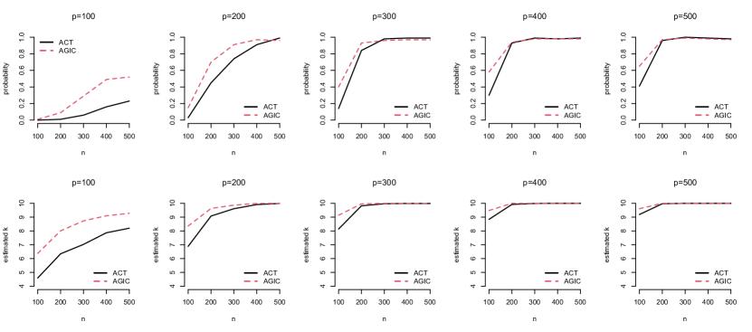
Figure 1: Performances of ACT and AGIC in Simulation 3 under varying $p,n$ with $k=10$.

Simulation 4 (the general spiked covariance model from Fan et al. (2022), large $p$, comparison with ACT). In this simulation, we set ${\mathbf{x}}\sim\mathcal{N}_{p}({\mathbf{0}},{\mathbf{\Sigma}})$, where ${\mathbf{\Sigma}}={\mathbf{Q}}{\mathbf{Q}}^{\top}+\mbox{Diag}\{\nu_{1}^{2},\ldots,\nu_{p}^{2}\}$. The matrix ${\mathbf{Q}}=(q_{ij})_{pk}$ is obtained as follows. For $1\leq j\leq 2$, let $q_{ij}$ be i.i.d. from $\textrm{N}(0,25)$ for $i\in 1,\ldots,\rho p$ and $q_{ij}$ be i.i.d. from Uniform(0,0.05) for $i\in\rho p+1,\ldots,p$. For $3\leq j\leq 5$, let $q_{ij}$ be i.i.d. from $\textrm{N}(0,1)$ for $i\in 1,\ldots,p$. Let $\nu_{1}^{2},\ldots,\nu_{p}^{2}$ be i.i.d. from Uniform(0, 180). We set $\rho=0.05$ and $k=5$. We compare AGIC with ACT. We also restrict the candidate spike size in the range of $k^{\prime}\in\{0,1,\ldots,20\}$. It can be seen from Figure 2 that, AGIC outperforms ACT, especially when $p$ or $n$ is relatively small (i.e., $p\leq 300$ or $n\leq 300$).

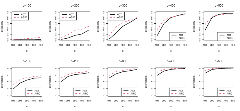
Figure 2: Performances of ACT and AGIC in Simulation 4 under varying $p,n$ with $k=5$.

5 Real-world data examples

In this section, we consider two real-world data examples on finance and biology respectively, and compare with existing methods including the PC₃ estimator proposed in Bai and Ng (2002), the ON₂ estimator proposed in Onatski (2009), the KN estimator proposed in Kritchman and Nadler (2008), the DDPA estimator proposed in Dobriban and Owen (2019), the ACT estimator proposed in Fan et al. (2022) and the BEMA estimator proposed in Ke et al. (2023).

5.1 The Fama-French 100 portfolios

We estimate the number of factors using the excess returns of Fama-French 100 portfolios. The well-known risk factors for equity markets are well explained by $k=3$ Fama-French factors: the market factor, the size factor and the value factor. We use the daily returns of 100 industrial Portfolios from January 2, 2010 to April 30, 2019. The dimension and the sample size of the dataset are $p=100$ and $n=2346$, respectively. When estimating $k$, AGIC selects $\hat{k}=3$, while PC₃, ON₂, KN, DDPA, BEMA and ACT estimate the number of factors as 8, 17, 45, 100, 6 and 3, respectively. It is seen that both AGIC and ACT correctly estimate the correct number of factors, while PC₃ and BEMA slightly overestimate the number of factors and ON₂, KN and DDPA more notably overestimate the number of factors.

In this data set, the 10 largest eigenvalues of the sample covariance matrix are 130.90, 5.48, 3.12, 1.53, 1.31, 0.99, 0.70, 0.61, 0.55, 0.51, respectively. The variance explained by 3 factors is $85.64\%$ due to a large spike top eigenvalue. The 10 largest eigenvalues of the sample correlation matrix are 80.62, 3.22, 2.06, 0.82, 0.75, 0.56, 0.37, 0.35, 0.31, 0.27, respectively and 3 factors explain $85.90\%$ total variation in 100 portfolios, while 8 factors and 6 factors explain $88.74\%$ and $88.02\%$ total variation, respectively.

5.2 The 1000 genomes project genotypes

Next, we illustrate our method on a genotype data from the 1000 Genomes Project (Phase III), publicly available at https://www.internationalgenome.org. We used Plink, a standard open-source whole genome association analysis software, to retain common variants with minor allele frequency greater than 0.1, and generated a set of variants in approximate linkage disequilibrium. The data pre-processing steps are performed following Zhong et al. (2022). We extracted a random subset of $p=2,000$ single-nucleotide polymorphisms (SNPs) from $n=500$ subjects.

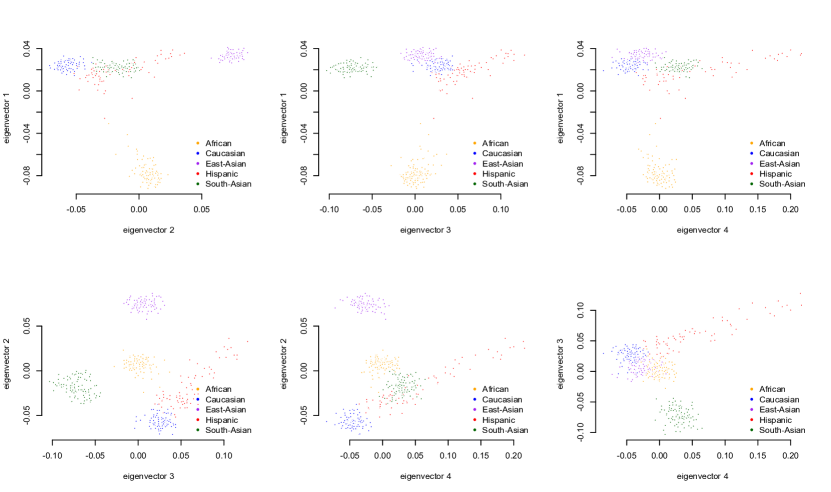
Figure 3: Plots of the top 4 left singular vectors of ${\mathbf{X}}$ from the 1000 Genomes Project data set.

Amongst these subjects, there are five self-reported ethnicity groups, including African, Caucasian, East Asian, Hispanic and South Asian. We treat these self-reported groups as the ground truth, which gives $k=4$. When estimating $k$, AGIC selects $\hat{k}=4$, while PC₃, ON₂, KN, DDPA, BEMA and ACT estimate $k$ as 3, 6, 6, 9, 4 and 6, respectively. The 10 largest eigenvalues of the sample covariance matrix are 134.18, 68.01, 23.76, 17.52, 8.19, 8.17, 7.89, 7.86, 7.80, 7.68, respectively. The variance explained by $\hat{k}=4$ is $12.20\%$ in 2000 variables, while $\hat{k}=3$, 6 and 9 explain $11.32\%$, $13.02\%$ and $14.20\%$ total variation, respectively. Figure 3 shows that the populations are well separated on the top 4 singular vectors.

6 Discussion

In this paper, we study limiting laws and consistent estimation criteria for the extreme eigenvalues in a spiked covariance model of dimension $p$. Our results are established under a general spiked covariance model, where the bulk eigenvalues are allowed to differ, and the number of spiked eigenvalues $k$ can diverge and the spiked eigenvalues need not be uniformly upper bounded or tending to infinity, as have been assumed in the existing literature.

We note that DDPA (Dobriban, 2020) and ACT (Fan et al., 2022) are proposed for selecting the number of factors in factor analysis, and their theoretical analyses are conducted under different settings. In factor analysis, the covariance matrix is assumed to take the form

$${\mathbf{\Sigma}}={\mathbf{\Psi}}{\mathbf{\Lambda}}{\mathbf{\Psi}}^{\top}+{\mathbf{\Phi}},$$

where ${\mathbf{\Psi}}$ is the $p\times k$ factor loading matrix, ${\mathbf{\Lambda}}$ is the covariance matrix of the factors, and ${\mathbf{\Phi}}$ is a diagonal matrix of idiosyncratic variances. For example, both DDPA and ACT require some form of the delocalization or sparsity condition on ${\mathbf{\Psi}}{\mathbf{\Lambda}}^{1/2}$. It is worth mentioning that in addition to factor analysis, Dobriban and Owen (2019) also investigated an application of the parallel analysis (PA) to selecting the number of significant components in a specific class of spiked covariance models, which enhanced the understanding of parallel analysis based factor selection methods. While identifying sufficient conditions that ensure the equivalence of factor selection in factor analysis and rank selection in PCA is a useful and important topic, it is beyond the scope of this paper, and we plan to investigate it in our future research.

References

- Abdi and Williams (2010) Abdi, H. and Williams, L. J. (2010), “Principal component analysis,” Wiley Interdisciplinary Reviews: Computational Statistics, 2, 433–459.
- Akaike (1974) Akaike, H. (1974), “A new look at the statistical identification model,” IEEE Transactions on Automatic Control, 19, 716–723.
- Anderson (2003) Anderson, T. W. (2003), An introduction to multivariate statistical analysis, Wiley, New York.
- Bai and Ng (2002) Bai, J. and Ng, S. (2002), “Determining the number of factors in approximate factor models,” Econometrica, 70, 191–221.
- Bai et al. (2018) Bai, Z. D., Choi, K., and Fujikoshi, Y. (2018), “Consistency of AIC and BIC in estimating the number of significant components in high-dimensional principal component analysis,” The Annals of Statistics, 46, 1050–1076.
- Bai and Ding (2012) Bai, Z. D. and Ding, X. (2012), “Estimation of spiked eigenvalues in spiked models,” Random Matrices: Theory and Applications, 1, 1150011.
- Bai and Silverstein (2004) Bai, Z. D. and Silverstein, J. W. (2004), “CLT for linear spectral statistics of large-dimensional sample covariance matrices,” The Annals of Probability, 32, 553–605.
- Bai and Yao (2008) Bai, Z. D. and Yao, J. F. (2008), “Central limit theorems for eigenvalues in a spiked population model,” Annales de l’Institut Henri Poincare (B) Probability and Statistics, 44, 447–474.
- Bai and Yao (2012) — (2012), “On sample eigenvalues in a generalized spiked population model,” Journal of Multivariate Analysis, 106, 167–177.
- Bao et al. (2022) Bao, Z., Ding, X., Wang, J., and Wang, K. (2022), “Statistical inference for principal components of spiked covariance matrix,” The Annals of Statistics, 50, 1144–1169.
- Buja and Eyuboglu (1992) Buja, A. and Eyuboglu, N. (1992), “Remarks on parallel analysis,” Multivariate behavioral research, 27, 509–540.
- Cai et al. (2020) Cai, T. T., Han, X., and Pan, G. (2020), “Limiting laws for divergent spiked eigenvalues and largest non-spiked eigenvalues of sample covariance matrices,” The Annals of Statistics,, 1255–1280.
- Chen and Li (2022) Chen, Y. and Li, X. (2022), “Determining the Number of Factors in High-dimensional Generalized Latent Factor Models,” Biometrika, 109, 769–782.
- Dobriban (2020) Dobriban, E. (2020), “Permutation methods for factor analysis and PCA,” The Annals of Statistics, 48, 2824–2847.
- Dobriban and Owen (2019) Dobriban, E. and Owen, A. (2019), “Deterministic parallel analysis: an improved method for selecting factors and principal components,” Journal of the Royal Statistical Society: Series B, 81, 163–183.
- Fan et al. (2022) Fan, J., Guo, J., and Zheng, S. (2022), “Estimating number of factors by adjusted eigenvalues thresholding,” Journal of the American Statistical Association, 852–861.
- Fan et al. (2018) Fan, J., Liu, H., and Wang, W. (2018), “Large covariance estimation through elliptical factor models,” Annals of statistics, 46, 1383.
- Jiang and Bai (2021) Jiang, D. and Bai, Z. (2021), “Generalized four moment theorem and an application to CLT for spiked eigenvalues of high-dimensional covariance matrices,” Bernoulli, 27, 274–294.
- Johansson (1998) Johansson, K. (1998), “On fluctuations of random Hermitian matrices,” Duke Mathematical Journal, 91, 151–203.
- Johnstone (2001) Johnstone, I. M. (2001), “On the distribution of the largest eigenvalue in principal component analysis,” The Annals of Statistics, 29, 295–327.
- Jonsson (1982) Jonsson, D. (1982), “Some limit theorems for the eigenvalues of a sample covariance matrix,” Journal of Multivariate Analysis, 12, 1–28.
- Ke et al. (2023) Ke, Z., Ma, Y., and Lin, X. (2023), “Estimation of the number of spiked eigenvalues in a covariance matrix by bulk eigenvalue matching analysis,” Journal of the American Statistical Association, 118, 374–392.
- Ke (2016) Ke, Z. T. (2016), “Detecting rare and weak spikes in large covariance matrices,” arXiv:1609.00883.
- Kritchman and Nadler (2008) Kritchman, S. and Nadler, B. (2008), “Determining the number of components in a factor model from limited noise data,” Chemometrics and Intelligent Laboratory Systems, 94, 19–32.
- Kritchman and Nadler (2009) — (2009), “Non-parametric detection of the number of signals, hypothesis tests and random matrix theory,” IEEE Transactions on Signal Processing, 57, 3930–3941.
- Li et al. (2020) Li, Z., Han, F., and Yao, J. (2020), “Asymptotic joint distribution of extreme eigenvalues and trace of large sample covariance matrix in a generalized spiked population model,” The Annals of Statistics, 3138–3160.
- Ma (2012) Ma, Z. (2012), “Accuracy of the Tracy-Widom limit for the extreme eigenvalues in the white Wishart matrices,” Bernoulli, 18, 322–359.
- Nadakuditi and Edelman (2012) Nadakuditi, R. R. and Edelman, A. (2012), “Sample Eigenvalues based detection of high-dimensional signals in white noise using relatively few samples,” IEEE Transactions on Signal Processing, 56, 2625–2638.
- Nadler (2010) Nadler, B. (2010), “Nonparametric detection of signals by information theoretic criteria: Performance analysis and an improved estimator,” IEEE Transactions on Signal Processing, 58, 2746–2756.
- Onatski (2009) Onatski, A. (2009), “Testing hypotheses about the number of factors in large factor models,” Econometrica, 77, 1447–1479.
- Onatski et al. (2013) Onatski, A., Moreira, M. J., and Hallin, M. (2013), “Asymptotic power of sphericity test for high-dimensional data,” The Annals of Statistics, 43, 1204–1231.
- Passemier et al. (2015) Passemier, D., Matthew, and Chen, Y. (2015), “Asymptotic linear spectral statistics for spiked Hermitian random matrices,” Journal of Statistical Physics, 160, 120–150.
- Passemier and Yao (2014) Passemier, D. and Yao, J. (2014), “Estimation of the number of spikes, possibly equal, in the high-dimensional case,” Journal of Multivariate Analysis, 127, 173–183.
- Paul (2007) Paul, D. (2007), “Asymptotics of sample eigenstructure for a large dimensional spiked covariance model,” Statistica Sinica, 17, 1617–1642.
- Saccenti and Timmerman (2017) Saccenti, E. and Timmerman, M. E. (2017), “Considering Horn’ parallel analysis from a random matrix theory point of view,” Psychometrika, 82, 186–209.
- Schwarz (1978) Schwarz, G. (1978), “Estimating the dimension of a model,” The Annals of Statistics, 6, 461–464.
- Silverstein (1995) Silverstein, J. W. (1995), “Strong convergence of the empirical distribution of eigenvalues of a large dimension random matrices,” Journal of Multivariate Analysis, 54, 331–339.
- Wang et al. (2014) Wang, Q., Silverstein, J., and Yao, J. (2014), “A note on the CLT of the LSS for sample covariance matrix from a spiked population model,” Journal of Multivariate Analysis, 130, 194–207.
- Wang and Yao (2013) Wang, Q. and Yao, J. (2013), “On the sphericity test with large-dimensional observations,” Electronic Journal of Statistics, 7, 2164–2192.
- Wang and Fan (2017) Wang, W. and Fan, J. (2017), “Asymptotics of empirical eigenstructure for high dimensional spiked covariance,” The Annals of Statistics, 45, 1342–1374.
- Wax and Kailath (1985) Wax, M. and Kailath, T. (1985), “Detection of signals by information theoretic criteria,” IEEE Transactions on Acoustics, Speech, and Signal Processing, 33, 387–392.
- Zhang et al. (2022) Zhang, Z., Zheng, Z., Pan, G., and Zhong, P. (2022), “Asymptotic independence of spiked eigenvalues and linear spectral statistics for large sample covariance matrices,” The Annals of Statistics, 50, 2205–2230.
- Zhao et al. (1986) Zhao, L. C., Krishnaiah, P. R., and Bai, Z. D. (1986), “On detection of the number of signals in presence of white noise,” Journal of Multivariate Analysis, 20, 1–25.
- Zhong et al. (2022) Zhong, X., Su, C., and Fan, Z. (2022), “Empirical Bayes PCA in high dimensions,” Journal of the Royal Statistical Society Series B: Statistical Methodology, 84, 853–878.