Exact long-range dielectric screening and interatomic force constants in quasi-2D crystals

Abstract

We develop a fundamental theory of the long-range electrostatic interactions in two-dimensional crystals by performing a rigorous study of the nonanalyticities of the Coulomb kernel. We find that the dielectric functions are best represented by $2\times 2$ matrices, with nonuniform macroscopic potentials that are two-component hyperbolic functions of the out-of-plane coordinate, $z$. We demonstrate our arguments by deriving the long-range interatomic forces in the adiabatic regime, where we identify a formerly overlooked dipolar coupling involving the out-of-plane components of the dynamical charges. The resulting formula is exact up to an arbitrary multipolar order, which we illustrate in practice via the explicit inclusion of dynamical quadrupoles. By performing numerical tests on monolayer BN, SnS₂ and BaTiO₃ membranes, we show that our method allows for a drastic improvement in the description of the long-range electrostatic interactions, with comparable benefits to the quality of the interpolated phonon band structure.

I Introduction

The separation of the interatomic force constants into short-range and long-range contributions has been a mainstay of lattice dynamics theory since the early 50s. Born and Huang (1954) The work of Cochran and Cowley Cochran and Cowley (1962) has established the correct form of the long-range part in the generic case of an anisotropic three-dimensional (3D) crystal, generalizing the earlier point-charge models. The treatment, however, remained phenomenological until the seminal work of Pick, Cohen and Martin Pick et al. (1970), where an analogous formula was derived in the context of first-principles theory, and the acoustic sum rule was formally demonstrated. The advantages of a rigorous derivation are numerous: on one hand, it paved the way for modern first-principles lattice dynamics, within the framework of density-functional perturbation theory; Zein (1984); Baroni et al. (1987); Gonze (1995a, b, 1997); Gonze and Lee (1997a); Baroni et al. (2001) on the other hand, it set the stage for further developments in linear-response methods, including higher-order generalizations of the Cochran-Cowley formula. Stengel (2013a); Royo et al. (2020)

The interest in lattice-dynamical properties of two-dimensional (2D) crystals has only started relatively recently. As a consequence, in spite of the remarkable progress of the past few years, the corresponding theoretical methods are not as mature as in the 3D case. To understand the nature of the problem (i.e., why traditional algorithms run into trouble in 2D), consider an insulating 2D crystal suspended in vacuum. A phonon propagating at some in-plane wavevector, ${\bf q}$, produces stray fields that decay asymptotically as $e^{-q|z|}$, where $q=|{\bf q}|$ and $z$ is the out-of-plane coordinate. This means that, for a small enough $q$, the macroscopic electrostatic potential perturbation spreads over a region of space that is much larger than the physical thickness of the material. Such a behaviour complicates the simulation of optical phonons in periodic boundary conditions, as the spurious interaction between repeated images leads to a physically incorrect description of the long-wavelength limit unless special precautions are taken.

To address this issue, the Coulomb cutoff technique Ismail-Beigi (2006); Rozzi et al. (2006) is now routinely used in first-principles calculations of phonons Sohier et al. (2017a) and related linear-response properties of suspended 2D systems. Such a treatment cures the pitfalls of a naive supercell-based calculation, and restores the correct physics in the small-$q$ limit by removing the undesired cross-talk between periodically repeated images. For example, the Coulomb cutoff nicely reproduces Sohier et al. (2017a) the physically correct Luca et al. (2020) behavior of longitudinal (LO) optical phonons, which are degenerate in frequency with the corresponding transverse (TO) modes right at the Brillouin zone center, and disperse linearly with $q$ in a vicinity of it. Sánchez-Portal and Hernández (2002); Michel and Verberck (2011)

While the methods to perform the electronic-structure calculations are under control, however, the theory of the long-range electrostatic interactions in two-dimensional crystals is still incomplete. Their fundamental understanding is crucial for the accurate interpolation of phonon bandstructures Sohier et al. (2017a); Royo et al. (2020) and electron-phonon matrix elements; Sohier et al. (2016, 2018); Li et al. (2019); Ma et al. (2020); Poncé et al. (2020); Deng et al. (2021) to model the interaction of individual layers with the dielectric environment (e.g., in layered heterostructures Andersen et al. (2015); Mohn et al. (2018); Sohier et al. (2021); Sponza and Ducastelle (2020)) and/or experimental probes; and to compute a number of important material properties that require a careful treatment of the electrostatics in the long-wavelength limit, such as flexoelectricity. Stengel (2013a, b); Stengel and Vanderbilt (2016); Royo and Stengel (2019); Springolo et al. (2020) Similar issues arise in the context of electron-electron interactions, Ando et al. (1982); Kotov et al. (2012) electronic excitations Freysoldt et al. (2008); Cudazzo et al. (2011); Berkelbach et al. (2013); Latini et al. (2015); Kylänpää and Komsa (2015); Hüser et al. (2013) and plasmonics Ando et al. (1982); Yan et al. (2011); Andersen et al. (2014); Ghosh et al. (2017); Agarwal et al. (2018). Only partial solutions where reported so far, by fitting the ab initio results to dielectric models, Sohier et al. (2017a) where oftentimes a strict 2D limit was assumed Cudazzo et al. (2011), or with the finite thickness of the real crystal heuristically accounted for. Freysoldt et al. (2008); Sohier et al. (2016, 2017a); Latini et al. (2015); Trolle et al. (2017) Systematic improvement of these models, e.g., along the lines of Ref. Royo et al., 2020, appears difficult unless a fundamental first-principles theory of the long-range interactions in quasi-2D crystals (that is, by explicitly treating the finite physical thickness of the material) is established.

Generalizing the approach of Ref. Pick et al., 1970 to the two-dimensional case, however, does not appear as an easy task. In a quasi-2D system the electrostatic interactions are much more complex to understand and describe than in 3D, due to the extreme anisotropy of the physics between the (extended) in-plane and (microscopic) out-of-plane directions. For instance, the usual tenet of 3D electrostatics of representing the macroscopic scalar potentials via structureless plane waves appears inappropriate to the quasi-2D case, where the exponential decay of stray fields in vacuum makes the problem inherently nonuniform along $z$. This implies, in the language of Ref. Pick et al., 1970, that the nonanalyticities of the Coulomb kernel in 2D are not simply restricted to the “head” of the inverse dielectric matrix, but concern an entire column of reciprocal-space vectors spanning the out-of-plane direction. Thus, separating long-range from short-range interactions, is per se a highly nontrivial issue in 2D, even at the level of the bare kernel (i.e., not considering the additional complications related to screening).

Here we solve the aforementioned challenges by introducing a number of key conceptual and methodological advances. First, we establish a rigorous and general separation between short-range and long-range electrostatic interactions in 2D, both by studying the nonanalytic properties of the Coulomb kernel, and via a physically more intuitive image-charge method. As a direct consequence of such range separation, the macroscopic electrostatic potentials in 2D emerge as two-component hyperbolic functions [$\cosh(qz)$ and $\sinh(qz)$] of the out-of-plane direction, $z$, reflecting the nonuniform nature of the long-range electrostatic fields. Remarkably, the Dyson equation for the screened Coulomb interaction reduces then to a linear-algebra problem involving $2\times 2$ matrices, i.e., is only marginally more complex than the scalar ($1\times 1$) inverse dielectric function that is characteristic of the 3D case. This result allows for a natural separation of the long-range electrostatic potentials into even and odd components with respect to $z\rightarrow-z$ reflection, and provides a unified description of both the intralayer couplings, as well as the interaction with external sources. The application of our formalism to the lattice-dynamical problem recovers the results of the existing dielectric models, but clearly goes beyond them, by (i) identifying a formerly overlooked contribution, i.e., the interaction between dipoles that are normal to the layer plane; by (ii) generalizing the theory to the next lowest order in ${\bf q}$ via incorporation of the dynamical quadrupole tensor; Royo and Stengel (2019) and by (iii) allowing for a more accurate description of the dielectric screening function. Finally, we demonstrate via extensive numerical tests on BN, SnS₂ and BaTiO₃ membranes that our formalism allows for a significant and systematic improvement in the existing methods for the theoretical study of phonons in 2D materials. Such an improvement comes at no additional cost from the computational perspective, and only requires a very minor addition to the existing codes.

This work is organized as follows. In Section II.1 and II.2 we introduce the basic concept of range separation in the context of the 3D dielectric matrix formalism of Pick, Cohen and Martin Pick et al. (1970) (PCM). In Section II.3 we present our main conceptual achievement, which consists in identifying the nonanalytic part of the Coulomb kernel in quasi-2D systems via an intuitive image-charge construction, and writing it as a $2\times 2$ small-space operator. In Section II.4 we discuss the physical significance of the hyperbolic basis functions that we use to represent the long-range Coulomb interactions. In Section II.5 we use these results to establish an exact formula for the long-range part of the force-constants matrix, and relate the materials-specific parameters to the Born effective charges, macroscopic dielectric tensor and dynamical quadrupoles as calculated within modern DFPT codes; the resulting Eq. (45) is another central achievement of this work. In Section II.6 we discuss the dependence of many useful quantities on the range-separation parameter, and its implications for a physically sound description of the dielectric function. The remainder of this work (Sec. III) is dedicated to the numerical implementation and tests of the formalism, and specifically of its performance in the Fourier interpolation of phonon bands.

II Theory

II.1 Range separation of the Coulomb interactions

Basic definitions. Within the adiabatic approximation, the screened Coulomb interaction $W$ links the screened potential, $V$, to an external charge perturbation, $\rho^{\rm ext}$, as

$$V({\bf r})=\int d^{3}r^{\prime}W({\bf r},{\bf r}^{\prime})\rho^{\rm ext}({\bf r^{\prime}}).$$ (1)

$W$ is, in turn, defined in terms of the bare Coulomb kernel, $\nu$, and the irreducible polarizability $\chi_{\rm ir}$,

$$W=(1-\nu\chi_{\rm ir})^{-1}\nu=(1+\nu\chi)\nu=\epsilon^{-1}\nu,$$ (2)

where $\epsilon=1-\nu\chi_{\rm ir}$ is the dielectric matrix. [The unity operator is a Dirac delta, $\delta({\bf r-r^{\prime}})$, in the real-space representation; it becomes a Kronecker delta over the reciprocal vectors in Fourier space.] $\chi_{\rm ir}$ linearly relates the (induced) charge response of the interacting electron system to the screened potential; within density-functional approaches it contains the effects of the exchange and correlation kernel, $f_{\rm xc}$, and can be defined in terms of the independent-particle polarizability ($\chi_{0}$) via a Dyson equation,

$$\chi_{\rm ir}=\chi_{0}+\chi_{0}f_{\rm xc}\chi_{\rm ir}=\chi_{0}(1-f_{\rm xc}\chi_{0})^{-1}.$$ (3)

By further incorporating dielectric screening effects we obtain the reducible polarizability, $\chi$,

$$\chi=\chi_{\rm ir}(1-\nu\chi_{\rm ir})^{-1}=\chi_{\rm ir}(1+\nu\chi)=\chi_{\rm ir}\epsilon^{-1}.$$ (4)

Range separation. The conceptual basis of our method consists in separating the bare Coulomb kernel into a short-range (SR) and a remainder long-range (LR) part,

$$\nu=\nu_{\rm sr}+\nu_{\rm lr}.$$ (5)

We shall assume that $\nu_{\rm sr}$ decays exponentially in real space or, equivalently, can be written as an analytic function of the wavevector ${\bf q}$ in reciprocal space; the nonanalytic part of $\nu$ is therefore contained in $\nu_{\rm lr}$. We can then define a screened short-range Coulomb interaction,

$$W_{\rm sr}=(1-\nu_{\rm sr}\chi_{\rm ir})^{-1}\nu_{\rm sr}=(1+\nu_{\rm sr}\chi_{\rm sr})\nu_{\rm sr},$$ (6)

and similarly an intermediate polarizability function, $\chi_{\rm sr}$, where the electrons interact via the exchange-correlation and short-range part of the Coulomb kernel,

$$\begin{split}\chi_{\rm sr}=&\chi_{0}+\chi_{0}(f_{\rm xc}+\nu_{\rm sr})\chi_{\rm sr}\\ =&\chi_{\rm ir}+\chi_{\rm ir}\nu_{\rm sr}\chi_{\rm sr}=\chi_{\rm ir}(1-\nu_{\rm sr}\chi_{\rm ir})^{-1}.\end{split}$$ (7)

The operator $\epsilon_{\rm sr}=1-\nu_{\rm sr}\chi_{\rm ir}$ is a short-range dielectric matrix, connecting the screened to the external potential at the $\nu_{\rm sr}+f_{\rm xc}$ level of interaction. We next define the screened long-range interaction as

$$W_{\rm lr}=(1-\nu_{\rm lr}\chi_{\rm sr})^{-1}\nu_{\rm lr}=(1+\nu_{\rm lr}\chi)\nu_{\rm lr},$$ (8)

where $\epsilon_{\rm lr}=1-\nu_{\rm lr}\chi_{\rm sr}$ can be regarded as a long-range dielectric matrix. Based on the above ingredients, one can show (a proof is provided in Appendix A) that the following relationship holds,

$$W=\epsilon_{\rm sr}^{-1}\,W_{\rm lr}\,(\epsilon_{\rm sr}^{-1})^{\dagger}+W_{\rm sr}.$$ (9)

This is the main formal result of this Section; an illustration of the idea is provided in Fig. 1. As we shall see shortly, Eq. (9) constitutes a generalization of the PCM approach, and recovers the latter as a special case.

Lattice dynamics. To see how this strategy works in the specific context of lattice dynamics, we shall combine the above results with the dielectric matrix formalism established in Ref. Pick et al. (1970). Consider a collective displacement of the sublattice $\kappa$ along $\alpha$ of the type

$$u^{l}_{\kappa\alpha}=\tau^{\bf q}_{\kappa\alpha}e^{i{\bf q\cdot R}_{l}},$$ (10)

where $l$ is a cell index and ${\bf R}_{l}$ span the real-space Bravais lattice. PCM’s formula for the dynamical matrix at a given point ${\bf q}$ in the Brillouin zone then reads, in our notation, as

$$\Phi^{\bf q}_{\kappa\alpha,\kappa^{\prime}\beta}=\bar{\Phi}^{\bf q}_{\kappa\alpha,\kappa^{\prime}\beta}-\delta_{\kappa\kappa^{\prime}}\sum_{\kappa^{\prime\prime}}\bar{\Phi}^{{\bf q}=0}_{\kappa\alpha,\kappa^{\prime\prime}\beta}.$$ (11)

($\kappa$, $\kappa^{\prime}$ and $\kappa^{\prime\prime}$ are basis indices, $\alpha$ and $\beta$ are Cartesian directions.) The matrix

$$\bar{\Phi}_{\kappa\alpha,\kappa^{\prime}\beta}=\langle\rho^{\rm ext}_{\kappa\alpha}|\,W\,|\rho^{\rm ext}_{\kappa^{\prime}\beta}\rangle$$ (12)

describes the bare nuclear interaction screened by the total dielectric function of the electrons at some wavevector ${\bf q}$, which we omit from now on to avoid overburdening the notation. The operator $W$ acts on the cell-periodic part of the “external” charge density, represented here as bra/kets. The latter, $|\rho^{\rm ext}_{\kappa\alpha}\rangle$, corresponds (see Appendix A) to the point dipoles that are induced by the nuclear displacement pattern of Eq. (10).

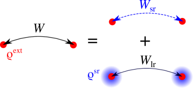
Figure 1: Decomposition of the screened Coulomb interaction according to Eq. (9). The full interaction ($W$) between bare external charges ($\rho^{\rm ext}$) is split into their mutual short-range interaction ($W_{\rm sr}$) plus the long-range interaction ($W_{\rm lr}$) between “dressed” charges ($\rho^{\rm sr}$).

The decomposition of the Coulomb kernel, Eq. (5), naturally leads via Eq. (9) to a similar partition of $\bar{\Phi}$ (and hence of the force-constants matrix, $\Phi_{\kappa\alpha,\kappa^{\prime}\beta}$),

$$\bar{\Phi}=\bar{\Phi}^{\rm sr}+\bar{\Phi}^{\rm lr},$$ (13)

where the short-range and long-range contributions are constructed according to Fig. 1,

$$\bar{\Phi}^{\rm sr}_{\kappa\alpha,\kappa^{\prime}\beta} =\langle\rho^{\rm ext}_{\kappa\alpha}|\,W_{\rm sr}\,|\rho^{\rm ext}_{\kappa^{\prime}\beta}\rangle,$$ (14a)

$$\bar{\Phi}^{\rm lr}_{\kappa\alpha,\kappa^{\prime}\beta} =\langle\rho^{\rm sr}_{\kappa\alpha}|\,W_{\rm lr}\,|\rho^{\rm sr}_{\kappa^{\prime}\beta}\rangle,$$ (14b)

Here $\rho^{\rm sr}_{\kappa\alpha}$ is the “dressed” charge-density response to an atomic displacement as calculated within the SR electrostatics,

$$|\rho^{\rm sr}_{\kappa\alpha}\rangle=(1+\chi_{\rm sr}\nu_{\rm sr})\,|\rho^{\rm ext}_{\kappa\alpha}\rangle.$$ (15)

The round bracket corresponds to the transpose of $\epsilon_{\rm sr}^{-1}$, which provides the formal connection between Eq. (13) and Eq. (9).

Small-space representation. Thus far, we have not made any specific assumption about $\nu_{\rm sr}$ and $\nu_{\rm lr}$, except that they sum up to $\nu$. For the practical advantages of Eq. (14) to become clear, it is necessary that $\nu_{\rm lr}$ enjoy a separable representation on a small set of basis functions,

$$\nu_{\rm lr}=\sum_{l,m=1}^{N}|\varphi_{l}\rangle\tilde{\nu}_{\rm lr}^{(lm)}\langle\varphi_{m}|,$$ (16)

We assume that the basis functions $|\varphi_{l}\rangle$ have an analytic dependence on ${\bf q}$, and are smooth on the scale of the interatomic spacings, consistent with their macroscopic character. This allows to express $\bar{\Phi}^{\rm lr}$ at any wavevector ${\bf q}$ of the Brillouin zone as a “small space” (see Ref. Martin et al., 2016, Chapter 7) linear-algebra problem of dimension $N$ (we use a tilde to distinguish small-space from full-space operators),

$$\bar{\Phi}^{\rm lr}_{\kappa\alpha,\kappa^{\prime}\beta}=\tilde{\rho}^{\rm sr\,*}_{\kappa\alpha}\cdot\tilde{W}_{\rm lr}\cdot\tilde{\rho}^{\rm sr}_{\kappa^{\prime}\beta},$$ (17)

where the long-range screened Coulomb interaction enjoys an analogous expression as in the full space,

$$\tilde{W}_{\rm lr}=(\underbrace{1-\tilde{\nu}_{\rm lr}\tilde{\chi}_{\rm sr}}_{\tilde{\epsilon}_{\rm lr}})^{-1}\tilde{\nu}_{\rm lr}.$$ (18)

The small-space operator $\tilde{\epsilon}_{\rm lr}$ acquires the physical meaning of a macroscopic dielectric matrix, and the material-dependent ingredients entering Eq. (17) and (18) are defined via projections on the basis functions,

$$\tilde{\rho}^{{\rm sr},(l)}_{\kappa\alpha}=\langle\varphi_{l}|\rho^{\rm sr}_{\kappa\alpha}\rangle,\qquad\tilde{\chi}_{\rm sr}^{(lm)}=\langle\varphi_{l}|\,\chi_{\rm sr}\,|\varphi_{m}\rangle.$$ (19)

These two quantities then provide a full description of the long-range electrostatics in the system.

Note that the above results can be easily applied to the range-separation of the scattering potential, $V_{\kappa\alpha}({\bf r})$, of interest in electron-phonon problems. By combining Eq. (1), (9) and (16), we find

$$V_{\kappa\alpha}({\bf r})=\sum_{l,m=1}^{N}\varphi^{\rm sr}_{l}({\bf r})\tilde{W}^{(lm)}_{\rm lr}\tilde{\rho}^{{\rm sr}}_{\kappa\alpha}+V_{\kappa\alpha}^{\rm sr}({\bf r}),$$ (20)

where $V_{\kappa\alpha}^{\rm sr}$ and $\varphi^{\rm sr}_{l}$ are the screened potential in response to the phonon [Eq. (10)] and to the external potential $\varphi_{l}$ [Eq. (21) below], respectively, at the SR level of interaction. Both $V_{\kappa\alpha}^{\rm sr}$ and $\varphi^{\rm sr}_{l}$ are, again, analytic functions of ${\bf q}$, which allows for their efficient interpolation over the Brillouin zone; they are available at no cost as by-product of the linear-response calculations that are required for the calculation of the dynamical matrix.

	$\varphi-\varphi$	$\varphi-\tau$	$\tau-\tau$	SCF kernel
noninteracting	$\chi_{0}$			$-$
irreducible	$\chi_{\rm ir}$			$f_{\rm xc}$
short-range	$\chi_{\rm sr}$	$\rho^{\rm sr}$	$\bar{\Phi}^{\rm sr}$	$f_{\rm xc}+\nu_{\rm sr}$
screened	$\chi$	$\rho$	$\Phi$	$f_{\rm xc}+\nu$

Table 1: Summary of the main response functions that we shall consider in this work, together with the SCF kernel that governs the electron-electron interactions in each case. The three central columns refer to the charge response to a scalar potential ($\chi$), the charge response to a phonon ($\rho$), or the atomic forces induced by a phonon ($\Phi$). [They can all be expressed as second derivatives of the energy with respect to scalar potential ($\varphi$) and/or phonon ($\tau$) perturbations.] $f_{\rm xc}$ is the exchange and correlation kernel; $\nu$ is the Coulomb kernel; for the meaning of the short-range (sr) label, see text.

Practical issues. In the framework of DFPT, the main response functions discussed in the above paragraphs (see Table 1 for a summary) can be recast as the second-order variation of the energy with respect to external parameters. The force-constants matrix, for instance, involves two phonon perturbations as defined in Eq. (10). Gonze and Lee (1997b); Baroni et al. (2001) The additional material properties that we have introduced in the above paragraphs can be computed by defining $N$ new perturbations of the type

$$V^{\rm ext}({\bf r})=\varphi_{l}^{\bf q}\,\varphi_{l}({\bf q},{\bf r})e^{i{\bf q\cdot r}}.$$ (21)

For the small-space polarizability ($\tilde{\chi}$) and charge-density response to a phonon ($\tilde{\rho}$) we have, then,

$$\tilde{\rho}^{(l)}_{\kappa\alpha}=\frac{1}{\Omega^{[d]}}\frac{\partial^{2}E}{\partial\varphi_{l}^{{\bf q}*}\partial\tau^{{\bf q}}_{\kappa\alpha}},\quad\tilde{\chi}^{(lm)}=\frac{1}{\Omega^{[d]}}\frac{\partial^{2}E}{\partial\varphi_{l}^{{\bf q}*}\partial\varphi_{m}^{{\bf q}}},$$ (22)

where $\Omega^{[d]}$ is the volume of the $d$-dimensional primitive cell.

The various “flavors” of each response function (irreducible, screened, etc.) are determined by the type of self-consistent (SCF) kernel that is used in the iterative solution of the linear-response problem (right column in Table 1). This is particularly convenient, as it avoids the need for explicitly solving the Dyson equations that govern dielectric screening at the microscopic level. Moreover, DFPT methods allow for a more straightforward incorporation of pseudopotentials, which are awkward to treat in the context of the dielectric matrix formalism [e.g., in Eq. (12) and (14a) the first-order nuclear potential is that of a point dipole, which implies an all-electron framework].

Crucially, both ingredients entering $\bar{\Phi}^{\rm lr}$, $\tilde{\rho}^{{\rm sr}}_{\kappa\alpha}$ and $\tilde{\chi}_{\rm sr}$, are analytic functions of ${\bf q}$, due to the assumed analyticity of $\nu_{\rm sr}$. This property is key in the perspective of an efficient and physically appealing representation of $\bar{\Phi}^{\rm lr}$, which can be achieved in two different ways:

• One explicitly calculates $\tilde{\rho}^{{\rm sr}}_{\kappa\alpha}$ and $\tilde{\chi}_{\rm sr}$ via Eq. (22), together with $\bar{\Phi}^{\rm sr}$, on a regular mesh of ${\bf q}$-points. These functions are then Fourier-interpolated at an arbitrary ${\bf q}$-point (this is guaranteed to converge quickly with the mesh resolution due to their analytic character), where $\bar{\Phi}^{\rm lr}$ and subsequently $\bar{\Phi}$ can be reconstructed exactly via Eq. (17) and Eq. (13).

• One seeks an approximate analytical expression (e.g. the dipole-dipole formula of Ref. Gonze and Lee (1997b)) for $\bar{\Phi}^{\rm lr}$ via a long-wave expansion of both $\tilde{\rho}^{{\rm sr}}_{\kappa\alpha}$ and $\tilde{\chi}_{\rm sr}$ (which is, again, allowed due to their analyticity) in a vicinity of the zone center. Typically, only few leading terms need to be retained for an accurate description of the long-range forces, and such quantities are straightforward to calculate within modern linear-response packages.  Gonze and Lee (1997a); Baroni et al. (2001)

In practice, we shall prefer the second option in the context of this work, as it only requires minor modifications to the existing code implementations.

II.2 The 3D case

As a first practical demonstration of our formalism, we shall now use it to rederive the classic results of PCM, valid for 3D crystals. Following PCM, we define $\nu_{\rm lr}$ as the ${\bf G}=0$ part of the Coulomb kernel in a vicinity of the zone center,

$$\nu_{\rm lr}({\bf G+q,G^{\prime}+q})=\delta_{{\bf G}0}\delta_{{\bf G}^{\prime}0}\frac{4\pi}{q^{2}}$$ (23)

Since the LR kernel vanishes except for a single Fourier component, the dimension of the “small space” is manifestly $N=1$, with structureless plane waves as basis functions, $\varphi({\bf r})=1$. This means that both $\tilde{\chi}_{\rm sr}$ and $\tilde{\rho}^{\rm sr}_{\kappa\alpha}$ are scalar functions of the wavevector ${\bf q}$. At the lowest order in ${\bf q}$, we have Pick et al. (1970)

$$\tilde{\chi}_{\rm sr} = -{\bf q}\cdot\bm{\chi}_{\rm mac}\cdot{\bf q}+\cdots,$$ (24)

$$\Omega\tilde{\rho}^{\rm sr}_{\kappa\alpha} = -i{\bf q}\cdot{\bf Z}_{\kappa\alpha}+\cdots,$$ (25)

where $\bm{\chi}_{\rm mac}$ and ${\bf Z}_{\kappa\alpha}$ are respectively the macroscopic dielectric susceptibility and Born effective charge tensors. (The tensorial components refer to the polarization direction; the dots stand for higher multipolar orders that are usually neglected – a detailed discussion of their significance can be found in Refs. Stengel, 2013a; Royo et al., 2020.) We have then, by using Eq. (8),

$$\tilde{W}_{\rm lr}=\frac{4\pi}{q^{2}}\left(1+\frac{4\pi}{q^{2}}{\bf q}\cdot\bm{\chi}_{\rm mac}\cdot{\bf q}+\cdots\right)^{-1},$$ (26)

which immediately leads, via Eq. (14b), to the established formula Pick et al. (1970) for the dipole-dipole interaction.

A disadvantage of the PCM method is that the separation between ${\bf G}=0$ and ${\bf G}\neq 0$ terms is only meaningful in a neighborhood of the zone center, and does not lend itself to a true range separation in real space. Within our formalism, it is easy to fix this limitation. We define the long-range Coulomb kernel as

$$\nu_{\rm lr}({\bf G+q,G^{\prime}+q})=\delta_{\bf GG^{\prime}}\frac{4\pi}{|{\bf G+q}|^{2}}e^{-\frac{|{\bf G+q}|^{2}}{4\Lambda^{2}}}.$$ (27)

The remainder, $\nu_{\rm sr}=\nu-\nu_{\rm lr}$, is regular at all ${\bf q+G}$, and is therefore short-ranged for any nonzero value of $\Lambda$. This corresponds to a range separation in real space in the following form,

$$\frac{1}{r}=\frac{{\rm erf}(r\Lambda)}{r}+\frac{{\rm erfc}(r\Lambda)}{r}.$$ (28)

If $\Lambda^{-1}$ is large enough (say, much larger than the lattice parameter), then $\nu_{\rm lr}$ only contains at most one nonzero element on the diagonal, while all other components can be discarded. This leads to a scalar long-range formula which is very similar to PCM’s (in fact, they coincide at the leading order in ${\bf q}$),

$$\tilde{W}_{\rm lr}=\frac{4\pi f(q)}{q^{2}}\left(1+\frac{4\pi f(q)}{q^{2}}{\bf q}\cdot\bm{\chi}_{\rm mac}\cdot{\bf q}+\cdots\right)^{-1},$$ (29)

but contains a Gaussian range-separation function,

$$f(q)=e^{-\frac{q^{2}}{4\Lambda^{2}}}.$$ (30)

The latter is reminiscent of the usual Ewald summation techniques Gonze and Lee (1997b) – and indeed, the formalism that we have developed in this Section can be regarded as a more sophisticated version of the Ewald method. It differs in spirit from the established approach in that the range separation is applied here a priori to the Coulomb kernel, and not a posteriori to the dipole-dipole expression of $\bar{\Phi}^{\rm lr}$ Gonze and Lee (1997b). Interestingly, such an approach results in a macroscopic dielectric function [round bracket of Eq. (29)] that explicitly depends on $\Lambda$ via $f(q)$; we shall come back to this point later on.

The remainder of this work will focus on how this technique can be generalized to systems with reduced dimensionality; in order to do this, we need to seek first of all an appropriate definition of $\nu_{\rm lr}$ in 2D.

II.3 Coulomb kernel in two dimensions

In quasi-2D crystals, it is convenient to separate the total momentum into in-plane (${\bf K}_{\parallel}={\bf G}_{\parallel}+{\bf q}$, where ${\bf G}_{\parallel}$ belongs to the reciprocal-space Bravais lattice, and ${\bf q}$ is the wave vector of the perturbation) and out-of-plane ($k_{z}$) components. Then the Coulomb kernel in open boundary conditions can be conveniently written as a function of the in-plane momentum and out-of-plane real-space coordinate $z$,

$$\nu({\bf K}_{\parallel},z-z^{\prime})=4\pi\int\frac{dk_{z}}{2\pi}\,\frac{e^{ik_{z}(z-z^{\prime})}}{K_{\parallel}^{2}+k_{z}^{2}}=2\pi\frac{e^{-K_{\parallel}|z-z^{\prime}|}}{K_{\parallel}}.$$ (31)

By analogy with the 3D case, one may be tempted to identify $\nu_{\rm lr}$ with the ${\bf G}_{\parallel}=0$ component of Eq. (31), which is clearly nonanalytic. Doing so, however, would be unfit to our purposes: unlike the ${\bf G}=0$ component of the Coulomb kernel in 3D, $\nu({\bf q},z-z^{\prime})$ is not a scalar, but an operator that depends nontrivially on $z$ and $z^{\prime}$. The practical appeal of the range separation method discussed in the previous Section rests on the representability of $\nu_{\rm lr}$ in a “small” space, where only one (as in the 3D case) or few physical degrees of freedom of macroscopic character are treated explicitly. The function $\nu({\bf q},z-z^{\prime})$ clearly violates such a condition.

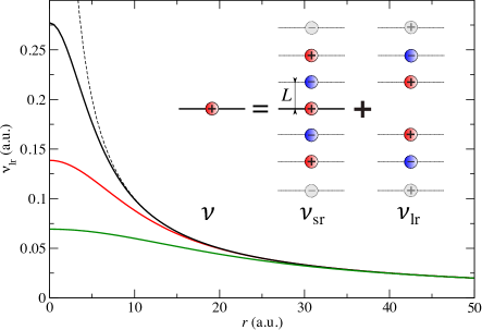
Figure 2: Real-space representation of the long-range Coulomb kernel as defined in the text. The curves correspond to the choices $L=5$ a.u. (black), $L=10$ a.u. (red) and $L=20$ a.u. (green). The Coulomb potential $1/r$ is shown as a dashed curve for comparison. The inset provides an intuitive illustration of the decomposition of Eq. (32) as an image-charge method.

To overcome this obstacle, and thereby achieve a sound separation between short-range and long-range interactions, we shall use the image-charge construction that is illustrated in Fig. 2 (inset). In particular, we shall define the short-range Coulomb kernel as follows,

$$\nu_{\rm sr}({\bf K}_{\parallel},z-z^{\prime})=\sum_{n}(-1)^{n}\nu({\bf K}_{\parallel},z-z^{\prime}-nL).$$ (32)

This consists in replacing an external charge perturbation (represented as a red circle with a “+” symbol in Fig. 2) with an infinite array of images, spaced by a distance $L$ along the out-of-plane direction and taken with alternating signs. We assume that the parameter $L$ is larger than the physical thickness of the layer, in such a way that neighboring images of the ground-state electronic density have vanishing overlap. For the same reason, we shall restrict our attention to the range $|z-z^{\prime}|<L$, which is the physically relevant regime for Coulombic interactions within the layer.

Clearly, $\nu_{\rm sr}$ is short-ranged, as the electrostatic potential produced by the linear array of alternating point charges vanishes exponentially for $r_{\parallel}\gg L$, where $r_{\parallel}$ is the in-plane distance from the array. Then, the long-range interactions must be entirely contained in $\nu_{\rm lr}$, which is defined via Eq. (5) as the remainder, $\nu_{\rm lr}=\nu-\nu_{\rm sr}$. To illustrate this fact, in the main panel of Fig. 2 we show a real-space representation of $\nu_{\rm lr}$ as it results from such a construction. As expected, $\nu_{\rm lr}$ deviates significantly from the Coulombic potential only for $r_{\parallel}<L$, where it avoids the $1/r_{\parallel}$ divergence of the latter and tends smoothly to a constant value instead.

The short-range Coulomb kernel as defined in Eq. (32) appears exotic at first sight, so the fact that it has been available for several decades in mainstream implementations of DFPT Giannozzi et al. (2009); Gonze et al. (2009) may come as a surprise to the reader. In a plane-wave electronic-structure code, suspended 2D crystals are routinely calculated by means of the supercell approach; this consists in repeating the system periodically along the vacuum direction, while setting the distance between images to some sufficiently large value, $L$, to avoid any unphysical cross-talk. As we anticipated in the introduction, long-wavelength phonons are problematic to simulate within such a computational setup, as spurious electrostatic interactions between images cannot be avoided in the ${\bf q}\rightarrow 0$ limit, unless special precautions (e.g., by means of the Coulomb truncation method) are taken Sohier et al. (2017b). Such unphysical interactions, however, can be exploited to our advantage, as they provide a straightforward first-principles implementation of Eq. (32). Indeed, a phonon traveling in the superlattice with momentum $(q_{x},q_{y},q_{z}=\pi/L)$, i.e., located at the Brillouin-zone boundary along the vacuum direction, introduces a phase delay of 180^∘ between neighboring images, which reproduces the alternating signs of our image-charge construction.

An explicit formula for $\nu_{\rm lr}$ can be derived by carrying out the summation of the $n\neq 0$ terms in Eq. (32). Due to our assumption of $|z-z^{\prime}|<L$, the argument $z-z^{\prime}-nL$ is defined negative for $n\geq 1$, and positive for $n\leq 1$. After a straightforward algebraic manipulation (see Appendix A) we arrive then at

$$\nu_{\rm lr}({\bf K}_{\parallel},z-z^{\prime})=\frac{2\pi f({K}_{\parallel})}{{K}_{\parallel}}\cosh[{K}_{\parallel}(z-z^{\prime})],$$ (33)

where the range-separation function in the prefactor is

$$f(K_{\parallel})=1-\tanh\left(\frac{K_{\parallel}L}{2}\right).$$ (34)

$f(K_{\parallel})$ is monotonously decreasing and vanishes exponentially for $K_{\parallel}\gg 1/L$: for a charge modulation of sufficiently short wavelength, the images do not “see” each other, as the stray fields decay faster than the vacuum thickness. In such a regime, the “zone-boundary” electrostatics coincides with the correct one and $\nu_{\rm lr}$, which is defined as the difference, vanishes. The parameter $L$ defines the length scale of the range separation (see the main panel of Fig. 2), and plays a similar role as the Gaussian width $\Lambda$ in Eq. (30). Note that $f(K_{\parallel})$ has a linear behavior ($f\simeq 1-K_{\parallel}L/2$) for small $K_{\parallel}$, which contrasts with the quadratic behavior of its 3D counterpart; we regard this outcome as a consequence of the reduced dimensionality. One can verify that Eq. (33) exactly reproduces the nonanalytic behavior of the full kernel, Eq. (31), at any order in ${\bf K}_{\parallel}$.

The hyperbolic cosine diverges exponentially for large arguments, which may raise some questions about the numerical stability of Eq. (33); also, one may wonder how we ended up with an unbounded potential when the original kernel of Eq. (31) is manifestly a bounded function of $|z-z^{\prime}|$ at any nonzero $q$. We stress that the cosh of Eq. (33) is really intended as a truncated hyperbolic cosine ($\nu_{\rm lr}$ is defined in the range $|z-z^{\prime}|<L$), in the same spirit of the Coulomb truncation method. Ismail-Beigi (2006); Rozzi et al. (2006); Sohier et al. (2016) (Our parameter $L$ corresponds to half the supercell length within the latter approach.) And, in fact, our definitions of $\nu_{\rm lr}$ and $\nu_{\rm sr}$, once represented on a plane-wave basis set, exactly sum up to the truncated Coulomb kernel as defined by Sohier et al. Sohier et al. (2016) (a formal proof is provided in Appendix C). Incidentally, our derivations show that Sohier’s method can also be understood as an image-charge construction: it only differs from $\nu_{\rm sr}$ by a factor $e^{-qL}$ in the odd-numbered terms of Eq. (32).

With these results in hand, we are now ready to attack the representability issue that we raised at the beginning of this Section. At first sight, it might seem that we haven’t made much progress – Eq. (33) is still expressed as a nontrivial function of $z$ and $z^{\prime}$. By using the elementary bisection formula of the hyperbolic cosine, however, one can equivalently write Eq. (33) as

$$\nu_{\rm lr}({\bf q},z-z^{\prime})=\bm{\varphi}(z)\cdot\tilde{\nu}_{\rm lr}({\bf q})\cdot\bm{\varphi}(z^{\prime}),$$ (35)

in terms of the small-space operator

$$\tilde{\nu}_{\rm lr}({\bf q})=\frac{2\pi f(q)}{q}\,\begin{pmatrix}1&0\\ 0&-1\end{pmatrix},$$ (36)

and the two-component macroscopic potential,

$$\bm{\varphi}(z)=\left[\cosh(qz),\sinh(qz)\right].$$ (37)

[We assume that $f(K_{\parallel})\simeq 0$ for any ${\bf G}_{\parallel}\neq 0$, leaving us with a simple ${\bf q}$-dependence of $\tilde{\nu}_{\rm lr}$.] Eq. (35) now provides the sought-after separable representation of the long-range Coulomb kernel. In spite of the apparent complexity of the electrostatic problem in 2D, with the extreme anisotropy of the physics between the in-plane and out-of-plane directions and the consequent inhomogeneity of the stray fields [here reflected in the nonuniform nature of the basis functions, Eq. (37)], we have managed to represent the long-range Coulomb interactions in a space whose dimensionality is only slightly larger than that of the trivial 3D case; we regard this as a remarkable conceptual achievement of this work.

The fact that the hyperbolic basis functions diverge exponentially with $z$ is, again, not an issue in practice, since our main focus is on intralayer interactions, occurring within a bounded region $|z-z^{\prime}|<L$. In the next Section we shall further corroborate their physical soundness by addressing the electrostatic potentials far away from the layer, which mediate its coupling to the dielectric environment and/or external probes.

II.4 Hyperbolic functions

To understand the physics that lies behind the two-component nature of the electrostatic potentials and operators, it is useful to recall some basic properties of the hyperbolic functions appearing in Eq. (37). The hyperbolic cosine is manifestly an even function of $z$, while the sine is odd: at the lowest order, the former reduces to an electric field acting parallel to the plane, while the latter corresponds to a perpendicular field. (To reflect this fact, we shall indicate the two components of the relevant matrices and vectors with the “$\parallel$” and “$\perp$” symbols henceforth.) This means that the cosh and sinh potentials mediate electrostatic interactions between charge densities that are, respectively, even and odd with respect to $z$-reflection. The emergence of a mirror-odd component marks a drastic departure from the 3D case, where transverse electric fields are forbidden by the translational periodicity of the crystal Hamiltonian. Based on the above, we can interpret the hyperbolic basis functions as the quasi-2D generalization of modulated electric fields, respectively oriented in-plane (cosh) or out-of-plane (sinh). This generalization is unique, as there is a unique solution to the Laplace equation in all space once the boundary condition at the $z=0$ plane is fully specified. This also means that the cosh and sinh functions constitute a complete basis for expanding an arbitrary electrostatic potential that is produced by external charges (i.e. located outside the volume of the layer).

As a consequence, the “small-space” representation of the perturbed charge density [Eq. (19)] must be relevant to describing not only the long-range interactions within the layer, but also the exponentially decaying vacuum fields outside the layer. To see this, consider an isolated 2D layer with a screened charge perturbation of the form

$$\rho^{\rm ext}({\bf r})=e^{i{\bf q\cdot r}}\rho^{\bf q}(z),$$ (38)

where $\rho^{\bf q}(z)$ is the planar average of the cell-periodic part. The electrostatic potential generated by $\rho^{\bf q}(z)$ can be written as a convolution in real space with the kernel of Eq. (31),

$$V^{\bf q}(z)=\int dz^{\prime}\,\nu({\bf q},z-z^{\prime})\rho^{\bf q}(z^{\prime}).$$ (39)

If we consider a point that is located far enough from the layer that the perturbed density vanishes, Eq. (39) reduces to

$$V^{\bf q}(z)=\frac{2\pi}{q}\left\{\begin{array}[]{lr}e^{-qz}\int dz^{\prime}\,e^{qz^{\prime}}\rho^{\bf q}(z^{\prime})&\text{for }z\gg 0,\\ e^{qz}\int dz^{\prime}\,e^{-qz^{\prime}}\rho^{\bf q}(z^{\prime})&\text{for }z\ll 0.\end{array}\right.$$ (40)

After observing that $e^{\pm qz}=\cosh(qz)\pm\sinh(qz)$, we obtain, for $|z|\gg 0$,

$$V^{\bf q}(z)=\frac{2\pi}{q}e^{-q|z|}\left[\rho^{\parallel}({\bf q})+{\rm sgn}(z)\rho^{\perp}({\bf q})\right],\\$$ (41)

where ${\rm sgn}(z)$ is the sign function, and we have defined the two-component charge-density perturbation by combining Eq. (19) with Eq. (37),

$$\rho^{\parallel}({\bf q})= \int dz\,\rho^{\bf q}(z)\cosh(qz),$$ (42a)

$$\rho^{\perp}({\bf q})= \int dz\,\rho^{\bf q}(z)\sinh(qz).$$ (42b)

This shows that the stray fields in the vacuum region are entirely specified by the “small space” representation of the screened charge density, thereby further substantiating its physical significance.

II.5 Long-range interatomic forces

In order to write the LR part of the dynamical matrix according to Eq. (14b) we shall define the small-space representations of the short-range polarizability ($\chi_{\rm sr}$) and charge-density response to a phonon ($\rho_{\kappa\alpha}^{{\rm sr}}$) by using Eq. (37) in conjunction with the formalism of Sec. II.1. Then, the observation that $\cosh(qz)$ and $\sinh(qz)/q$ are both analytic functions of ${\bf q}$ naturally leads to a long-wave expansion of $\tilde{\chi}_{\rm sr}$ and $\tilde{\rho}^{\rm sr}$. Regarding $\tilde{\chi}_{\rm sr}$, we have

$$\tilde{\chi}_{\rm sr}({\bf q})=-\begin{pmatrix}{\bf q}\cdot\bm{\alpha}^{\parallel}\cdot{\bf q}&q{\bm{\beta}}\cdot{\bf q}\\ q{\bm{\beta}}\cdot{\bf q}&q^{2}\alpha^{\perp}\end{pmatrix}+O(q^{4}),$$ (43)

where we have introduced the in-plane ($\bm{\alpha}^{\parallel}$) and out-of-plane ($\alpha^{\perp}$) macroscopic polarizabilities of the layer, and ${\beta}_{m}$ denotes the off-diagonal elements that couple in-plane and out-of-plane dipoles; their relation to the macroscopic dielectric tensor of the supercell is described in Appendix B. Note that these relationships are exact, i.e. they do not rely on any assumption regarding the physical properties of the layer, unlike the dielectric model of Ref. Sohier et al., 2016.

The charge-response functions, on the other hand, can be conveniently expanded as

$$\tilde{\rho}^{\rm sr,\parallel}_{\kappa\alpha}({\bf q})= -\frac{iq_{\beta}}{\sqrt{S}}\underbrace{\left[\hat{Z}^{(\beta)}_{\kappa\alpha}-i\frac{q_{\gamma}}{2}\left(\hat{Q}^{(\beta\gamma)}_{\kappa\alpha}-\delta_{\beta\gamma}\hat{Q}^{(zz)}_{\kappa\alpha}\right)+\cdots\right]}_{\mathcal{Z}^{(\beta)}_{\kappa\alpha}({\bf q})}$$

$$\times e^{-i{\bf q}\cdot\bm{\tau}_{\kappa}},$$ (44a)

$$\tilde{\rho}^{\rm sr,\perp}_{\kappa\alpha}({\bf q})= \frac{q}{\sqrt{S}}\underbrace{\left[\hat{Z}^{(z)}_{\kappa\alpha}-iq_{\beta}\hat{Q}^{(z\beta)}_{\kappa\alpha}+\cdots\right]}_{\mathcal{Z}^{\perp}_{\kappa\alpha}({\bf q})}e^{-i{\bf q}\cdot\bm{\tau}_{\kappa}},$$ (44b)

where $S$ is the cell surface [see Eq. (58)], the complex phase is a structure factor that depends on the in-plane location of the atom $\kappa$ within the cell, and we have indicated as $\hat{\bf Z}_{\kappa\alpha}$ and $\hat{\bf Q}_{\kappa\alpha}$ the dynamical dipole and quadrupole tensors in 2D. These generally differ from their standard definitions in 3D (see Appendix B for details): (i) the electrical boundary conditions are set to short circuit in plane, and open circuit along $z$, consistent with the “zone-boundary” electrostatics; (ii) the Cartesian moments along $z$ are calculated with respect to the $z=0$ plane, which corresponds to the center of the 2D layer.

The way $\hat{Q}^{(zz)}_{\kappa\alpha}$ enters Eq. (44), which stems from the asymptotic expansion of the hyperbolic cosine, $\cosh(qz)\simeq 1+q^{2}z^{2}/2$, might appear surprising at first sight. To see its physical significance note that, in classical electrostatics, only the traceless part of the Cartesian multipole tensor Applequist (1989) produces long-range electrostatic fields (see Appendix D). In two dimensions, this implies that the diagonal elements of the quadrupolar tensor only contribute to the long-range forces via their difference, consistent with Eq. (44); we regard this outcome as a further demonstration of the internal consistency of our theory.

While the above formalism is entirely general, for simplicity we shall focus henceforth on 2D crystals that enjoy a mirror plane at $z=0$. This assumption implies that the off-diagonal component of the polarizability, ${\beta}_{m}$, vanishes by symmetry, and the diagonal elements of the screened Coulomb interactions can be treated as two separate scalar problems. By plugging the long-wave expansions of the densities, Eq. (44), and the dielectric functions, Eq. (43), into Eq. (17), we obtain the following formula for the long-range interatomic forces,

$$\bar{\Phi}^{\rm lr}_{\kappa\alpha,\kappa^{\prime}\beta}({\bf q})=\frac{2\pi f(q)}{Sq}\left(\frac{({\bf q}\cdot\bm{\mathcal{Z}})^{*}_{\kappa\alpha}\,({\bf q}\cdot\bm{\mathcal{Z}})_{\kappa^{\prime}\beta}}{\tilde{\epsilon}_{\parallel}({\bf q})}-q^{2}\frac{\mathcal{Z}^{\perp*}_{\kappa\alpha}\,\mathcal{Z}^{\perp}_{\kappa^{\prime}\beta}}{\tilde{\epsilon}_{\perp}({\bf q})}\right)e^{-i{\bf q}\cdot(\bm{\tau}_{\kappa^{\prime}}-\bm{\tau}_{\kappa})}.$$ (45)

where

$$\tilde{\epsilon}_{\parallel}({\bf q}) =1+\frac{2\pi f(q)}{q}{\bf q}\cdot({\bm{\alpha}}^{\parallel}+\cdots)\cdot{\bf q},$$ (46a)

$$\tilde{\epsilon}_{\perp}({\bf q}) =1-2\pi qf(q)\,(\alpha^{\perp}+\cdots).$$ (46b)

$\tilde{\epsilon}_{\parallel}$ and $\tilde{\epsilon}_{\perp}$ refer to the diagonal components of the small-space dielectric matrix, $\tilde{\epsilon}_{\rm lr}$. At leading order in ${\bf q}$, they correspond, respectively, to the monopolar and dipolar response functions that were considered in earlier works Andersen et al. (2015); Sohier et al. (2021); the dots stand for the terms $O(q^{4})$ and higher in Eq. (43). $\mathcal{Z}$ are the dynamical dipoles, corresponding to the square brackets in Eq. (44), which generally depend on ${\bf q}$ via quadrupolar and higher-order terms. Eq. (45) describes the long-range electrostatic interactions exactly up to an arbitrary multipolar order; this is the second central result of this work.

By truncating the expansions of Eq. (43) and Eq. (44) to their leading orders in ${\bf q}$, we recover an approximate representation of the long-range force constants that can be directly compared with earlier works on the subject. The mirror-even part of Eq. (45) is consistent with the formula proposed by Sohier et al. Sohier et al. (2017a), with the most obvious difference that the range-separation function $f(q)$ in the prefactor is replaced a Gaussian, $g(q)=e^{-\frac{q^{2}}{4\Lambda}}$, therein. Both functions tend to unity at ${\bf q}=0$ and may therefore appear equivalent at first sight. Our $f(q)$ as given by Eq. (34), however, displays a linear (rather than quadratic) dependence at small $q$, which is key to reproducing the nonanalytic behavior of the long-range Coulomb kernel exactly. Interestingly, in our formula $f(q)$ also appears in the definition of the dielectric function, Eq. (46); we shall come back to this point in the following Section.

The mirror-odd part (second term in the round bracket) of Eq. (45) is, to the best of our knowledge, an original result of this work. (The contribution of the out-of-plane dipoles to the long-range potentials discussed by Ref. Deng et al. (2021) has mirror-even quadrupolar character, and therefore is qualitatively different; see Appendix B for further details.) Remarkably, the interaction between out-of-plane dipoles enters with a negative sign, which originates from Eq. (36). To rationalize this outcome, note that an unsupported insulating film imposes open-circuit electrical boundary conditions on out-of-plane dipoles, which implies that, at ${\bf q}=0$, optical phonon modes experience a full depolarizing field along $z$. Such physics is well described by the “zone-boundary” electrostatics that we discussed earlier. When moving away from $\Gamma$, the spatial modulation of the dipole moments acts as an effective Yukawa-like screening, which progressively weakens the effects of the depolarizing field; the physics is not dissimilar to the driving force towards domain formation in low-dimensional ferroelectrics. As we shall see in the results section, this implies that the ZO branch (optical modes with polarization out of plane) approaches ${\bf q}=0$ with a linear dispersion, similarly to LO modes but with a negative slope. Remarkably, in the mirror-odd component of the dielectric function, Eq. (46), the out-of-plane polarizability of the layer also enters with negative sign, which implies that $\epsilon^{\perp}({\bf q})$ is always smaller than one. This outcome might bear intriguing connections to the theory of negative capacitance Zubko et al. (2016) effects in thin-film ferroelectrics; we regard this as a fascinating topic to explore in future studies.

II.6 The range separation parameter

As we have mentioned earlier, an interesting outcome of our derivations is that the small-space dielectric function, $\tilde{\epsilon}_{\rm lr}$, explicitly depends on the range-separation parameter via $f(q)$. In particular, the $f(q)$ prefactor suppresses the polarizability contribution at large momenta, and $\tilde{\epsilon}_{\rm lr}({\bf q})$ tends to unity for $q\gg L^{-1}$ (i.e., at length scales where the physics of the dielectric screening is microscopic in character). This behavior is common to both the 2D [Eq. (46)] and the 3D [Eq. (29)] cases, i.e., it does not depend on dimensionality but appears to be a general consequence of the formalism developed in Sec. II.1. The appearance of a fictitious parameter ($L$ or $\Lambda$) may appear undesirable; it is, however, a natural manifestation of the arbitrariness in the separation between what we regard as “macroscopic” and “local field” effects, which is inherent to our strategy. This issue is well known in other contexts: e.g., in the “nanosmoothing” techniques Junquera et al. (2007); Baldereschi et al. (1988) that are used to extract macroscopic physical information from microscopic first-principles data; or in the popular Ewald method, which can be regarded as a straightforward application of our formalism to a system of classical point charges.

In the case of the mirror-odd component, the progressive suppression of the polarizability contribution for increasing $q$ is not only a direct consequence of the above arguments, but is also an essential ingredient for a mathematically stable description of the long-range interactions. Indeed, the contribution of the layer polarizability $\alpha^{\perp}$ enters with a negative sign, which would lead to a vanishing denominator in Eq. (45) if $f(q)$ were neglected (i.e., set to unity) in Eq. (46). One can show that the stability condition is

$$L>4\pi\alpha_{\perp}.$$ (47)

By recalling the definition of $\alpha_{\perp}$, Eq. (66), one quickly realizes that the above condition marks the crossover between a positive and a negative value of $\epsilon_{zz}^{-1}$, the inverse dielectric constant of the hypothetical cell of thickness $L$ that we use to represent our 2D crystal. Thus, assuming a “strict 2D limit” (e.g., following the guidelines of Ref. Cudazzo et al., 2011) would be unphysical in the context of the out-of-plane dielectric function: an infinitesimally thin layer with a finite out-of-plane polarizability would inevitably lead to divergencies in the screened Coulomb interaction at short distances. In the language of Sec. II.1, one can equivalently say that the small-space operator $\tilde{\epsilon}_{\rm lr}$ must be an invertible matrix for our method to be physically sensible and mathematically stable; the above considerations show that $L$ must be chosen wisely for this condition to hold.

As a matter of fact, all analytic response functions that one calculates within the SR Coulomb kernel depend on $L$ implicitly via the $L$-dependence of the latter. This raises the obvious question of whether the small-momentum expansion coefficients of $\tilde{\rho}^{\rm sr}$ [Eq. (44)] and/or $\tilde{\chi}_{\rm sr}$ [Eq. (43)] are affected by this issue. One can show that the lowest orders in ${\bf q}$ of either function, including all quantities that are explicitly mentioned in Eq. (44) and Eq. (43), are independent of $L$; their respective $L$-dependence kicks in at the octupolar level for $\tilde{\rho}^{\rm sr}$ and at $O(q^{4})$ for $\tilde{\chi}_{\rm sr}$. The 2D and 3D cases are, again, qualitatively similar in these regards: a demonstration that the quadrupolar moments are independent of the range-separation parameter (a fictitious Thomas-Fermi screening length was used) in 3D crystals, while octupoles are not, can be found, respectively in Ref. Martin (1972) and Ref. Stengel (2013a).

Of course, the screened counterparts of the charge-density response and polarizability must be independent of $L$, consistent with their definition in free-boundary conditions. Interestingly, we have

$$\tilde{\rho}_{\kappa\alpha}({\bf q}) =\tilde{\epsilon}_{\rm lr}^{-1}({\bf q})\,\tilde{\rho}^{\rm sr}_{\kappa\alpha}({\bf q}),$$ (48a)

$$\tilde{\chi}({\bf q}) =\tilde{\epsilon}_{\rm lr}^{-1}({\bf q})\,\tilde{\chi}_{\rm sr}({\bf q}).$$ (48b)

This means that the implicit $L$-dependence of the SR quantities (which originates from the modifications to the short-range Coulomb kernel that a variation of $L$ entails) cancels out exactly with an analogous dependence of $\epsilon$ when the former are divided by the latter. Such a cancellation becomes only approximate when the multipolar representations of both $\rho^{\rm sr}$ and $\epsilon$ are truncated, and such a deviation can be used to gauge the overall accuracy of the method.

	B	N	Sn	S(1)	Ba(1)	Ti	O(1)	O(2)	O(3)
$Z_{\kappa x}^{(x)}$	2.685	$-$2.685	4.814	$-$2.407	2.946	6.603	$-$2.487	$-$2.285	$-$5.237
$Z_{\kappa z}^{(z)}$	0.246	$-$0.246	0.343	$-$0.171	0.482	0.947	$-$0.675	$-$0.280	$-$0.280
$Q_{\kappa x}^{(xy)}$	4.261	0.384		3.700
$Q_{\kappa y}^{(xx)}$	4.261	0.384		3.700
$Q_{\kappa y}^{(yy)}$	$-$4.261	$-$0.384		$-$3.700
$Q_{\kappa y}^{(yz)}$				$-$0.298	1.356		$-$0.972
$Q_{\kappa z}^{(xx)}$				$-$2.932	$-$24.552		21.641
$Q_{\kappa z}^{(zz)}$				0.231	4.605		$-$3.868
$\alpha_{\parallel}$	1.882		6.629		4.461
$\alpha_{\perp}$	0.310		0.720		0.900

Table 2: Cartesian components of dynamical dipole, quadrupole and polarizability tensors (in the “zone-boundary” electrostatics). Atomic units are used; only linearly independent coefficients are shown. The numbering of the atoms refers to the convention of Fig. 3.

III Results

We shall now benchmark the performance of our method regarding the Fourier interpolation of the dynamical matrix elements and eigenvalues (phonon bands). Our computational model consists in the three materials illustrated in Fig. 3, i.e., in two representative 2D monolayer crystals, BN and SnS₂, and a thin membrane of BaTiO₃. (The latter consists in a tetragonal stacking of three BaO/TiO₂/BaO layers, the relaxed structure being non piezoelectric.) To start with, we shall present the calculated physical parameters for our materials set.

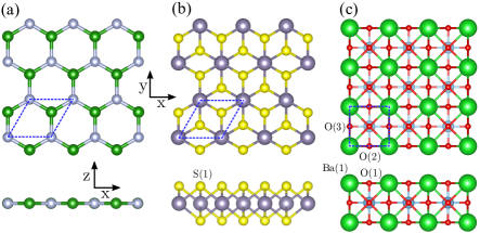
Figure 3: Atomic structure of the simulated 2D materials: BN (a), SnS₂ (b), BaTiO₃ (c).

III.1 Calculation of the physical constants

Our calculations are performed within the local-density approximation as implemented in ABINIT Romero et al. (2020), by using optimized norm-conserving Vanderbilt pseudopotentials Hamann (2013) from the PseudoDojo. van Setten et al. (2018) For all the materials considered, we use a plane-wave cutoff of 80 Hartree and a $12\times 12\times 1$ ${\bf k}$-point grid. The length of the supercell in the out-of-plane $z$-direction is set to 40 Bohr in all cases. Before performing the linear-response calculations, we optimize the atomic positions and cell parameters of the unperturbed systems to a stringent tolerance ($10^{-8}$ and $10^{-6}$ atomic units for residual stress and forces, respectively). The linear-response quantities (dielectric tensor, dynamical charges Gonze and Lee (1997b) and quadrupoles Royo and Stengel (2019)) necessary to build the LR dynamical matrix are then computed with the DFPT and longwave drivers of ABINIT Romero et al. (2020) and subsequently transformed to the zone-boundary electrostatics following the recipe of Appendix B. The results are reported in Table 2.

III.2 Interpolation of the dynamical matrix

We shall now test the performance of our method regarding the Fourier-interpolation of the phonon bands. In particular, we shall benchmark the results of our interpolation method, against the exact DFPT phonon frequencies and the frequencies obtained by means of the phenomenological 2D Fourier interpolation of Sohier et al. Sohier et al. (2017a) both accessible via the Quantum Espresso Giannozzi et al. (2009, 2017) (QE) suite. In the course of our tests, we have detected a missing factor of $2\pi/a_{0}$ in the QE subroutine (version 6.5) that builds the long-range interactions following the guidelines of Ref. Sohier et al. (2017a). Such a factor likely passed unnoticed in earlier works, Sohier et al. (2017a) as it is close to one (in atomic Bohr units) in all materials studied therein. For a fair comparison, in the following we shall present results obtained after having fixed this issue. (Our fix will be incorporated in future releases of the software, presumably starting from v.6.8.)

To calculate the dynamical matrices we use the “Coulomb truncation” method Ismail-Beigi (2006) as implemented Sohier et al. (2016, 2017b) in the linear-response module of QE. For consistency, we use the same computational parameters, exchange and correlation functionals and pseudopotentials as in our ABINIT calculations (see Sec. III.1). Prior to performing the actual calculations, we carefully check the compatibility between ABINIT and Quantum Espresso calculations by comparing the main linear-response quantities (polarizabilities and Born effective charges) that can be obtained through both packages, obtaining essentially no differences (within a tolerance of four significant digits).

Once the dynamical matrices are calculated on a discrete mesh (${\bf q}_{i}$) of points spanning the 2D Brillouin zone of the crystal, we evaluate the approximate (A) long-range interactions, $\bar{\Phi}^{\rm lr,A}_{\kappa\alpha,\kappa^{\prime}\beta}({\bf q}_{i})$, via the truncated Eq. (45) on the same 2D mesh, and use it to define an approximate short-range part as

$$\Phi^{\rm sr,A}({\bf q}_{i})=\Phi({\bf q}_{i})-\Phi^{\rm lr,A}({\bf q}_{i}).$$ (49)

[$\Phi^{\rm lr,A}$ is obtained from $\bar{\Phi}^{\rm lr,A}$ after enforcing translational invariance via Eq. (11).] Finally, $\Phi^{\rm sr,A}_{\kappa\alpha,\kappa^{\prime}\beta}({\bf q}_{i})$ is Fourier-interpolated to obtain the short-range dynamical matrix at an arbitrary ${\bf q}$, and eventually the full dynamical matrix once the long-range part $\Phi^{\rm lr,A}_{\kappa\alpha,\kappa^{\prime}\beta}({\bf q})$ is added back to it. Again, $\bar{\Phi}^{\rm lr,A}_{\kappa\alpha,\kappa^{\prime}\beta}({\bf q})$ only depends on $L$ (the only free parameter) via the range-separation function $f(q)$ that is contained in Eq. (45) and Eq. (46).

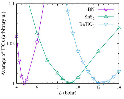
Figure 4: Average of short-range IFCs (absolute value excluding self-interactions) as a function of the $L$ parameter used to generate the long-range dynamical matrices. For each of the three materials studied in this work the y-axis data have been scaled by the minimum calculated value.

To determine the optimal value of $L$, we estimate the accuracy of the interpolation at a given $L$ by requiring that the decay of the “sr” force constants in real space be as fast as possible. In practice, we define an indicator by summing up the absolute values of the short-range IFCs in real space,

$$d(L)=\sum^{\prime}_{\kappa\kappa^{\prime}\,l}\sum_{\alpha\beta}|\Phi^{\rm sr,A}_{\kappa\alpha,\kappa^{\prime}\beta}(0,l)|,$$ (50)

where the prime means that self-interactions are excluded. The minimum of $d(L)$ yields then the sought-after value of $L$. This only entails a minimal computational burden, since it only requires recalculating $\bar{\Phi}^{\rm lr,A}_{\kappa\alpha,\kappa^{\prime}\beta}({\bf q})$ several times at different values of $L$. This is done at the level of the post-processing program (i.e., it does not imply running additional linear-response calculations). The results for our tested materials are shown in Fig. 4. For BN, we checked that the value of $L$ optimized via Eq. (50) is consistent with our conclusions based on the analysis of the screened charge, following the guidelines of Sec. II.6.

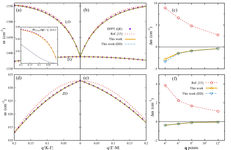
Figure 5: BN. Dispersion of the LO, TO (a–b) and ZO (d–e) phonon branches in the long-wavelength limit along the K–$\Gamma$ [(a) and (d)] and $\Gamma$–M [(b) and (e)] segments in the 2D Brillouin zone. The curves show the results of the 2D Fourier interpolation method of Ref. Sohier et al., 2017a as implemented in Quantum Espresso after having corrected the bug in the implementation (see text), and of the method developed in this work, either with or without (DD) dynamical quadrupoles; exact [DFPT (QE)] phonon frequencies are shown as circles. All interpolations are performed on a grid of $8\times 8$ in-plane q points. (c) and (f) show the absolute error resulting from the different interpolation methods as a function of the q-mesh density for the LO and ZO branches, respectively. DFPT frequencies are taken as reference, and the error is evaluated at the q point lying halfway between $\Gamma$ and the first commensurate q point along the $\Gamma$–M segment. The inset in (a) shows the element of the $\Gamma$-modes representation of the force-constants matrix [Eq. (51)] that describes the coupling between the TO and LO modes along the K–$\Gamma$ segment. Absolute values divided by the modulus of q are represented.

III.2.1 BN

We begin by applying our scheme to study the long-wavelength dispersion of the optical phonons in monolayer BN. Phonons in BN have been the subject of several works in the framework of tight-binding models Sánchez-Portal and Hernández (2002), classical potentials Michel and Verberck (2011); Jiang et al. (2018) or first-principles electronic-structure theory; Wirtz et al. (2003); Sohier et al. (2017a) therefore, this material constitutes an excellent first benchmark for our method. Fig. 5 shows the results obtained with our Fourier interpolation formalism and using a value of $L=4.5$ Bohr which, as anticipated in the previous section and confirmed by the data represented in Fig. 4, is optimal in order to minimize the spread of the IFCs. Compared with the bands obtained by following the interpolation of Sohier et al., Sohier et al. (2017a) our method manifestly improves the description of both the LO and ZO branches, accurately reproducing the exact DFPT frequencies.

Regarding the LO mode, we ascribe this improvement to our more accurate treatment of the long-range 2D screening function, while the inclusion of dynamical quadrupoles appears to have a minor impact on the interpolated LO frequencies. To see this, we repeated the interpolation procedure while neglecting dynamical quadrupoles in $\bar{\Phi}^{\rm lr,A}$ (dot-dashed blue curves in Fig. 5), obtaining negligible differences. For a more quantitative comparison, we show in Figs. 5(c) the deviation from the exact LO branch as a function of the q-mesh resolution: our method is highly accurate already at a coarse $4\times 4$ mesh, while earlier treatments result in a much slower convergence.

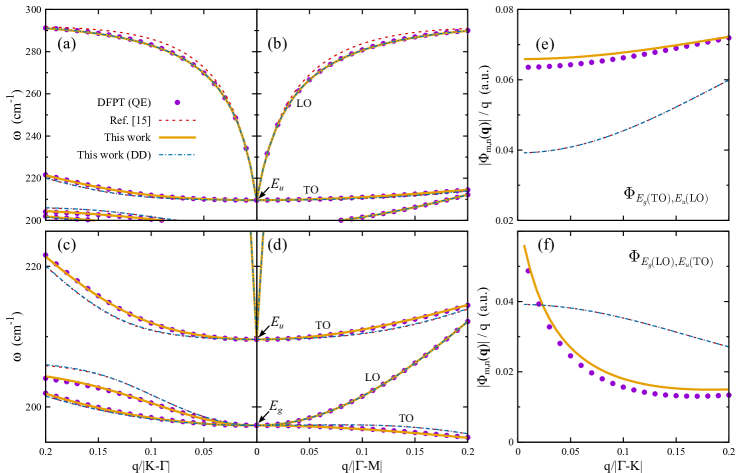
Figure 6: SnS₂. (a-b): Dispersion of the optical $E_{u}$ branches in the long-wavelength limit along the K–$\Gamma$ (a) and $\Gamma$–M (b) segments in the 2D Brillouin zone. (c–d): Dispersion of the lower-energy $E_{u}$ and the two $E_{g}$ branches along the K–$\Gamma$ (c) and $\Gamma$–M (d) segments. Interpolations are performed on a grid of $8\times 8$ in-plane q points. (e-f): Elements of the $\Gamma$-modes representation of the force-constants matrix corresponding to the $E_{g}$(TO)–$E_{u}$(LO) (e) and $E_{g}$(LO)–$E_{u}$(TO) (f) couplings along the $\Gamma$–K segment. Absolute values divided by $|{\bf q}|$ are shown.

The seemingly negligible impact of the dynamical quadrupoles in the interpolation of the LO frequencies is surprising, so we decided to investigate this point further. We find that the quadrupolar terms are important to reproduce the correct interactions between modes, corresponding to the off-diagonal elements of the dynamical matrix, in the long-wavelength limit. To illustrate this point, we project the force-constants matrix at a given wavevector, ${\bf q}$, onto the $\Gamma$-point mode eigenvectors ($u^{m}_{\kappa\alpha}$, $m$ being a mode index), appropriately modulated by a position-dependent complex phase,

$$\Phi_{m,n}({\bf q})=\langle u^{m}_{\kappa\alpha}|e^{-i\,{\bf q}\cdot\bm{\tau}_{\kappa}}\Phi_{\kappa\alpha,\kappa^{\prime}\beta}({\bf q})\,e^{i\,{\bf q}\cdot\bm{\tau}_{\kappa^{\prime}}}|u^{n}_{\kappa^{\prime}\beta}\rangle.$$ (51)

In the inset of Fig. 5(a) we plot the off-diagonal element of $\Phi_{m,n}({\bf q})$, quantifying the strength of the coupling between the LO and TO modes, along a portion of the K–$\Gamma$ segment. As above, we compare the exact DFPT values with the results of the Fourier interpolation, which we perform either including or excluding the contribution of the dynamical quadrupoles. Clearly, the quadrupoles play a crucial role in ensuring that the long-wave limit is accurately described. Note the qualitative error of the dipole-dipole interpolation, which approaches $\Gamma$ quadratically instead of linearly. As a matter of fact, the specific treatment of the dipole-dipole terms has no effect on the coupling between these two modes. All the models (except that including the dynamical quadrupoles), or even a complete neglect of the long-range interactions during the interpolation, yield exactly the same result [see inset of Fig. 5(a)].

Regarding the ZO branch of Fig. 5(d–e), note its characteristic linear dispersion when approaching the $\Gamma$ point, which is reminiscent of the LO branch except for the (negative) sign of the group velocity. This behavior, as we mentioned earlier, stems from the out-of-plane dipole-dipole interactions, which were neglected in earlier works. Indeed, when such interactions are left untreated, as in the dashed curves of Fig. 5(d–e), the Fourier interpolation results a quadratic dispersion, and a discrepancy that decays very slowly with the q-mesh resolution [Fig. 5(f)]. Our method clearly reproduces the qualitatively correct physics in the long-wavelength limit, with an excellent match between the interpolated and exact frequencies already at the coarsest mesh resolution that we have considered [Fig. 5(f)]. Note that dynamical quadrupoles are irrelevant here, since their effect on the mirror-odd part of the electrostatics vanishes by symmetry.

III.2.2 SnS₂

SnS₂ has been the focus of several studies lately, both in its bulk Zhen and Wang (2020) and monolayer Shafique et al. (2017) forms. Its main interest lies in the very low lattice thermal conductivity, He et al. (2018) which is important for thermoelectric efficiency. Clearly, an accurate representation of phonon frequencies is key to these applications, which motivates its consideration as a representative testcase. Note that in the case of SnS₂, a larger (compared to BN) value of $L=9$ bohr yields an optimally fast decay of the IFCs (see Fig. 4) and has been therefore used in the interpolation.

Fig. 6 shows the dispersion of the four (out of six) optical branches that are lowest in energy. The modes of Fig. 6(a–b) originate from the doubly degenerate $E_{u}$ mode at the $\Gamma$ point, with a calculated frequency of $\omega(E_{u})=$210 cm^-1, and correspond to the LO and TO modes with in-plane polarization. Similarly to the BN case, our interpolation scheme has a most visible impact on the highest LO mode, where our improved treatment of screening results in an excellent match with the exact DFPT frequencies. Again, the effect of quadrupoles appears to be unimportant for the interpolation of the LO branch, which is very well described already at the dipole-dipole level.

In Fig. 6(c–d) we show, on a magnified vertical scale, the TO branch of the aforementioned $E_{u}$ doublet, together with two additional branches deriving from the Raman-active $E_{g}$ modes [$\omega(E_{g})=$197 cm^-1]. Here, contrary to the above examples, the inclusion of dynamical quadrupoles is important to reproduce the correct phonon dispersion. This can be clearly appreciated by the comparison with the results of the lower-order models (limited to dipole-dipole interactions), which significantly deviate from the exact DFPT frequencies. The latter, on the other hand, are matched by the full electrostatic model with excellent accuracy.

To understand the reason why the dipole-dipole model is inaccurate for these bands, we have quantified the quadrupolar strength of each mode along the two relevant $\hat{\bf q}$-directions, by projecting the calculated components of $Q_{\kappa\alpha}^{(\beta\gamma)}$ on the corresponding $\Gamma$-point eigenvectors. Interestingly, the largest discrepancies between the two electrostatic models are observed along the branches where dynamical quadrupoles vanish by symmetry, which might appear counterintuitive at first sight. However, one must keep in mind that Fourier interpolation is a global operation on the 2D Brillouin zone. This means that residual nonanalyticities in the “short-range” dynamical matrix affect the quality of all interpolated branches, including those that are not directly concerned by macroscopic electric fields. It turns out that, similarly to the BN case, the inclusion of dynamical quadrupoles significantly improves the description of the off-diagonal matrix elements, which in SnS₂ couple $E_{g}$(TO) with $E_{u}$(LO) [Fig. 6(e)] and $E_{g}$(LO) with $E_{u}$(TO) [Fig. 6(f)] when moving away from $\Gamma$. Here, the impact on the phonon frequencies is much larger than in BN because the relative closeness in energy of the interacting branches amplifies the effect. We have likewise confirmed that dipole-dipole interactions play no role in interpolating these off-diagonal matrix elements.

Note that two additional optical branches, respectively of $A_{g}$ and $A_{u}$ symmetry, are present at higher energies (not shown); the electrostatic corrections, while present, have a relatively lesser impact on their interpolated frequencies.

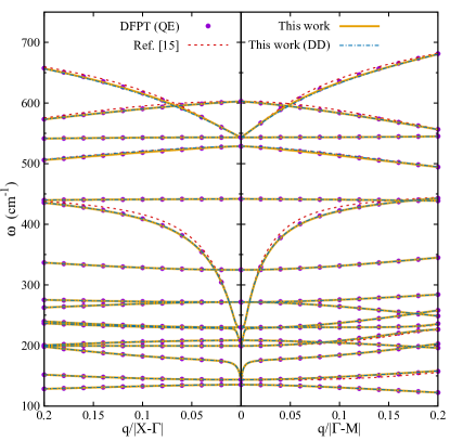
Figure 7: BaTiO₃ membrane. Dispersion of the optical phonon branches in the long-wavelength limit along the X–$\Gamma$ and $\Gamma$–M segments. The interpolated frequencies are obtained from the dynamical matrices calculated on a grid of $8\times 8$ in-plane q points.

III.2.3 BaTiO₃ membrane

Our motivation for studying a thin perovskite membrane as a showcase for our method stems from the recent surge of interest in such systems. This rapidly growing area of research has been fueled by the experimental breakthroughs in the preparation of unsupported oxide films via sacrifical layers. Di Lu et al. (2016) The main advantage resides in the unprecedented possibility of studying the impact of reduced size on the properties of perovskite crystals, and on the unprecedented degree of control over the mechanical boundary conditions that a membrane geometry allows. Hong et al. (2020) The theoretical study of the phonon spectrum, a mainstay of the current understanding of 3D complex oxides, provides a unique view on the effects of dimensionality on, e.g., the stability of the lattice against a ferroelectric distortion. We shall provide a practical demonstration in the following.

Fig. 7 shows the dispersion of the optical phonons as obtained from the three different interpolation methods that we introduced in the previous paragraphs. We have used an optimal value of $L$=12.0 bohr, once again extracted by minimizing Eq. (50) as shown in Fig. 4. Many of the trends that we have already observed for BN and SnS₂ crystals are manifestly present: i) the highly dispersive LO modes are most affected by the improvements brought about by our new formalism, concretely by the enhanced treatment of screening; ii) the ZO branches exhibit a linear dispersion in long-wavelength limit, requiring explicit treatment of the out-of-plane DD interactions for its qualitatively correct representation; iii) the effect of the dynamical quadrupoles is minimal, and only barely appreciable in the dispersion of the second-highest ZO branch. Interestingly, our interpolation scheme results in an improved description of selected transverse optical branches as well. We believe that the discrepancies produced by the existing scheme might be a “collateral damage” of its inaccurate description of the LO branches: our 2D BaTiO₃ crystal appears to be a case where the small-${\bf q}$ dip in the dispersion of some LO modes is particularly pronounced, possibly affecting the corresponding TO branches as well.

The physical origin of this rather extreme behavior resides in the ferroelectric low-energy mode of BaTiO₃, which is characterized by an abnormally large dipolar strength, $Z_{l}$. (Recall that the linear dispersion coefficient of the dynamical matrix eigenvalues close to $\Gamma$ is proportional to the square of $Z_{l}$. Sohier et al. (2017a)) Interestingly, the minimal thickness of the film prevents this mode from going “soft” at any point in the 2D Brillouin zone (our centrosymmetric structure is, therefore, at least a metastable configuration of the crystal), pointing to a complete suppression of ferroelectricity in the ultrathin limit. Studying the crossover between 2D and 3D physics as a function of slab thickness in this system will be an exciting topic for future studies. In this perspective, we expect the virtues of our interpolation method to become even more manifest as thickness increases. Indeed, the near-surface dynamical quadrupoles in our scheme grow linearly with thickness because of the dipolar contribution in Eq. (67), and eventually might become crucially important for a qualitatively correct interpolation.

IV Conclusions

In summary, we have developed a rigorous analytical description of the long-range electrostatic screening and interatomic forces in two-dimensional crystals, within a fundamental first-principles context. As a first application, we have used it to develop an explicit formula, exact up to the quadrupolar order, for the long-range part of the interatomic force constants. Numerical tests on selected materials demonstrate its superior accuracy in the interpolation of the phonon bands, at no extra cost compared to the existing schemes.

Our formalism provides a general platform for treating long-range electrostatics in 2D systems, with an applicability that goes well beyond the specifics of lattice dynamics. First, one could use Eq. (20) to reconstruct the nonanalytic contributions to the scattering potential in electron-phonon calculations, in a similar spirit as in Refs. Brunin et al., 2020a, b; Jhalani et al., 2020; Park et al., 2020. Second, the results of Sec. II.4 should allow for a natural incorporation of our formalism into dielectric models of layered systems, e.g., in combination with the methods of Refs. Andersen et al. (2015); Mohn et al. (2018); Sohier et al. (2021); Sponza and Ducastelle (2020). The exact 2D representation of the macroscopic dielectric function of an arbitrarily thick layer makes our approach particularly appealing in this context, as it does not require any approximation (e.g., to the monopolar/dipolar interactions Andersen et al. (2015); Sohier et al. (2021)), or limiting assumption (e.g., about the separable character of the ground-state wave functions Sponza and Ducastelle (2020)). In turn, our exact treatment of higher-order order multipolar couplings could facilitate the description and modeling of advanced electromechanical effects, such as flexoelectricity. Springolo et al. (2020) Also, one could generalize the calculation of the 2D polarizability functions, $\chi({\bf q})$, to finite frequencies, and thereby facilitate the use of modern many-body perturbation techniques in low-dimensional systems. Freysoldt et al. (2008); Felipe et al. (2020) In a materials context, our methods appear well suited to treating emergent systems that lie at the crossover between 2D and 3D, such as oxide membranes, which are attracting a rapidly growing experimental interest. Finally, generalizing our approach to one-dimensional nanowires could be another exciting topic for follow-up studies.

Appendix A Supporting analytical derivations

Proof of Eq. (9). By using the results and definitions of Sec. II.1, and in particular by recalling that $\chi_{\rm sr}\epsilon_{\rm lr}^{-1}=\chi$, we find

$$\begin{split}(\underbrace{1+\nu_{\rm sr}\chi_{\rm sr}}_{\epsilon_{\rm sr}^{-1}})&W_{\rm lr}\underbrace{(1+\chi_{\rm sr}\nu_{\rm sr})}_{(\epsilon_{\rm sr}^{-1})^{\dagger}}=\\ =&(\epsilon_{\rm lr}^{-1}+\nu_{\rm sr}\chi_{\rm sr}\epsilon_{\rm lr}^{-1})\nu_{\rm lr}(1+\chi_{\rm sr}\nu_{\rm sr})\\ =&(1+\nu_{\rm lr}\chi+\nu_{\rm sr}\chi)\nu_{\rm lr}(1+\chi_{\rm sr}\nu_{\rm sr})\\ =&(1+\nu\chi)\nu_{\rm lr}(1+\chi_{\rm sr}\nu_{\rm sr})\\ =&\underbrace{(1+\nu\chi)\nu}_{W}-(1+\nu\chi)\nu_{\rm sr}+(1+\nu\chi)\nu_{\rm lr}\chi_{\rm sr}\nu_{\rm sr}.\end{split}$$ (52)

We are left to show that the second and third terms on the rhs sum up to $-W_{\rm sr}$,

$$\begin{split}(1+\nu\chi)\nu_{\rm sr}-(1+\nu\chi)&\nu_{\rm lr}\chi_{\rm sr}\nu_{\rm sr}=\\ =&(1+\nu\chi)(\underbrace{1-\nu_{\rm lr}\chi_{\rm sr}}_{\epsilon_{\rm lr}})\nu_{\rm sr}\\ =&\epsilon_{\rm lr}\nu_{\rm sr}+\nu\chi_{\rm sr}\nu_{\rm sr}\\ =&\nu_{\rm sr}-\nu_{\rm lr}\chi_{\rm sr}\nu_{\rm sr}+\nu\chi_{\rm sr}\nu_{\rm sr}\\ =&W_{\rm sr}.\end{split}$$ (53)

Plane-wave representation of Eq. (12). We shall work with the cell-periodic part of functions and operators at a certain wavevector ${\bf q}$ in the Brillouin zone. We shall set the normalization conventions for the forward Fourier transform in 3D as

$$f({\bf G})=\frac{1}{\sqrt{\Omega}}\int_{\rm cell}d^{3}re^{-i{\bf G\cdot r}}f({\bf r}),$$ (54)

where $f$ is a generic cell-periodic function (not to be confused with the range-separation function defined in the main text), and ${\bf G}$ belongs to the reciprocal-space Bravais lattice of the crystal. In other words, we use a basis for our full-space operators of the type

$$\langle{\bf r}|{\bf G}\rangle=\frac{1}{\sqrt{\Omega}}e^{i{\bf G\cdot r}}.$$ (55)

On such a basis, the external charge of Eq. (12) reads as

$$\langle{\bf G}|\rho^{\rm ext}_{\kappa\alpha}\rangle=-i\frac{Z_{\kappa}}{\sqrt{\Omega}}({\bf G+q})_{\alpha}e^{i{\bf G}\cdot\bm{\tau}_{\kappa}},$$ (56)

and the bare Coulomb kernel is

$$W({\bf G+q},{\bf G^{\prime}+q})=\delta_{\bf GG^{\prime}}\frac{4\pi}{|{\bf G+q}|^{2}}.$$ (57)

With these definitions, our Eq. (12) coincides with Eq. (4.5) of PCM.

In two dimensions, we use a mixed representation where the in-plane components are treated in reciprocal space, while the out-of-plane coordinate is treated in real space. The Fourier transform then reads as

$$f({\bf G}_{\parallel},z)=\frac{1}{\sqrt{S}}\int_{\rm cell}dxdye^{-i{\bf G_{\parallel}\cdot r}}f({\bf r}),$$ (58)

where $S$ is the cell surface.

Proof of Eq. (33). By combining Eq. (32) and Eq. (31), our definition of $\nu_{\rm lr}=\nu-\nu_{\rm sr}$ reads as

$$\nu_{\rm lr}({\bf K}_{\parallel},z-z^{\prime})=-\frac{2\pi}{K_{\parallel}}\sum_{n\neq 0}(-1)^{n}e^{-K_{\parallel}|z-z^{\prime}-nL|}.$$ (59)

Based on the assumption that $|z-z^{\prime}|<L$, this can be written as

$$\begin{split}\nu_{\rm lr}({\bf K}_{\parallel},z-z^{\prime})=&-\frac{2\pi}{K_{\parallel}}\left(e^{K_{\parallel}|z-z^{\prime}|}+e^{-K_{\parallel}|z-z^{\prime}|}\right)\\ &\times\sum_{n=1}^{+\infty}(-1)^{n}e^{-nK_{\parallel}L}.\end{split}$$ (60)

The sum can be simplified by using the formula for the geometric power series, converging for $|x|<1$,

$$\frac{1}{1-x}=1+x+x^{2}+x^{3}+\cdots$$ (61)

We arrive at

$$\nu_{\rm lr}({\bf K}_{\parallel},z-z^{\prime})=\frac{2\pi}{K_{\parallel}}\cosh[K_{\parallel}(z-z^{\prime})]\frac{2e^{-K_{\parallel}L}}{1+e^{-K_{\parallel}L}},$$ (62)

which coincides with Eq. (33).

Appendix B Dipoles, quadrupoles and polarizabilities in 2D

In the following, we shall discuss how the physical quantities entering Eq.(44) and Eq. (43) are related to the Born dynamical charges ($Z^{(\alpha)}_{\kappa\beta}$), dynamical quadrupoles ($Q^{(\alpha\gamma)}_{\kappa\beta}$) and macroscopic clamped-ion dielectric tensor ($\epsilon_{\alpha\beta}$) that are calculated via standard linear-response techniques Gonze and Lee (1997b); Royo and Stengel (2019) in a supercell geometry. [The macroscopic dielectric tensor of a 3D crystal, $\epsilon_{\alpha\beta}$, should not be confused with the small-space dielectric function, $\tilde{\epsilon}_{\rm lr}({\bf q})$, that we define and use in the main text.] There are two main differences that one needs to take into account: (i) the electrical boundary conditions (EBC) are not the same, since the quantities entering Eq. (43) and Eq. (44) are intended to be calculated within the “zone-boundary” electrostatics, while the standard implementation of $Z^{(\alpha)}_{\kappa\beta}$, $Q^{(\alpha\gamma)}_{\kappa\beta}$ and $\epsilon_{\alpha\beta}$ assumes 3D short-circuit boundary conditions (as obtained by removing the nonanalytic ${\bf G}=0$ term from the Coulomb kernel); and (ii) the multipole moments are assumed to be taken with respect to the $z=0$ symmetry plane, rather than the unperturbed atomic location.

Regarding the Born charges and dielectric polarizabilities, one only needs to worry about (i), since they are both dipolar in character and hence origin-independent. The in-plane Born charges are unaltered by the EBC, i.e. for $\alpha=x,y$ we have

$$\hat{Z}^{(\alpha)}_{\kappa\beta}=Z^{(\alpha)}_{\kappa\beta}.$$ (63)

Conversely, along the out-of-plane direction the so-called “Callen charges” must be used, consistently with the open-circuit EBC that the reference zone-boundary electrostatics imposes along $z$,

$$\hat{Z}^{(z)}_{\kappa\beta}=\frac{Z^{(z)}_{\kappa\beta}}{\epsilon_{zz}}.$$ (64)

The macroscopic polarizabilities of the 2D layer can be calculated via

$$\alpha^{\parallel}_{\alpha\beta} = \frac{L}{4\pi}(\epsilon_{\alpha\beta}-1),$$ (65)

$$\alpha^{\perp} = \frac{L}{4\pi}(1-\epsilon_{zz}^{-1}).$$ (66)

(The indices $\alpha\beta$ run over the two in-plane components.) Note that the parameters $\hat{\bf Z}_{\kappa\beta}$, $\bm{\alpha}^{\parallel}$ and $\alpha^{\perp}$ are all independent of the vacuum thickness (provided that the electron density of neighboring images has negligible overlap), as required for well-defined materials properties. The above results are consistent with the prescriptions of Refs. Sohier et al. (2016, 2017a); Tian et al. (2020): our work puts them on firmer theoretical grounds, by identifying them with the exact limiting behavior of well-defined response functions.

Devising the conversion rules for the dynamical quadrupoles is slightly more delicate, as different components mix up in a way that is not always intuitive. Regarding the the mixed and out-of-plane components, one has

$$\hat{Q}^{(z\alpha)}_{\kappa\beta} =\frac{Q^{(z\alpha)}_{\kappa\beta}+\tau_{\kappa z}Z^{(\alpha)}_{\kappa\beta}}{\epsilon_{zz}},$$ (67a)

$$\hat{Q}^{(zz)}_{\kappa\beta} =\frac{Q^{(zz)}_{\kappa\beta}+2\tau_{\kappa z}Z^{(z)}_{\kappa\beta}}{\epsilon_{zz}}.$$ (67b)

The dielectric constant at the denominator relates to the EBC change, analogously to the above discussion of the Born effective charges. The addition of the Born effective charge times the $z$ coordinate of the atom at the numerator, on the other hand, takes care of the origin shift. Indeed, the dynamical quadrupoles within DFPT can be written as a second moment of the charge density induced by an atomic displacement as Stengel (2013a)

$$Q^{(\alpha\gamma)}_{\kappa\beta}=\int d^{3}r\,\rho_{\kappa\beta}({\bf r})\,({\bf r}-\bm{\tau}_{\kappa})_{\alpha}({\bf r}-\bm{\tau}_{\kappa})_{\gamma}.$$ (68)

One can then break down the $z$-components of the round brackets as

$$({\bf r}-\bm{\tau}_{\kappa})_{z}=z-{\tau}_{\kappa z},$$ (69)

and after recalling that the Born charge can also be defined as a real-space moment,

$$Z^{(\alpha)}_{\kappa\beta}=\int d^{3}r\,\rho_{\kappa\beta}({\bf r})\,({\bf r}-\bm{\tau}_{\kappa})_{\alpha},$$ (70)

one quickly arrives at Eq. (67). We are only left with working out the in-plane components, which can be readily converted as

$$\hat{Q}^{(\alpha\gamma)}_{\kappa\beta}={Q}^{(\alpha\gamma)}_{\kappa\beta}-4\pi\chi_{\alpha\gamma}\hat{Q}^{(zz)}_{\kappa\beta},$$ (71)

where $\chi_{\alpha\beta}$ are the in-plane components of the macroscopic dielectric susceptibility tensor of the supercell. It is interesting to note that the enforcement of the correct electrical boundary conditions for a suspended 2D layer already endows the in-plane quadrupoles with a contribution from the $(zz)$ component, $\hat{Q}^{(zz)}_{\kappa\beta}$. Because of this, the traceless component that appears in Eq. (44) enjoys a particularly simple expression,

$$\hat{Q}^{(\alpha\gamma)}_{\kappa\beta}-\delta_{\alpha\gamma}\hat{Q}^{(zz)}_{\kappa\beta}=Q^{(\alpha\gamma)}_{\kappa\beta}-\epsilon_{\alpha\gamma}\hat{Q}^{(zz)}_{\kappa\beta}.$$ (72)

One can show that all the components of $\hat{\bf Q}_{\kappa\beta}$ are all independent of the vacuum thickness, $L$, unlike those of ${\bf Q}_{\kappa\beta}$.

Interestingly, a contribution of the out-of-plane dipoles to the electron-phonon matrix elements involving the $A^{\prime}_{1}$ branch of MoS₂ was recently identified in Ref. Deng et al. (2021). The above results nicely clarify the physical nature of the reported mechanism: the out-of-plane dipoles contribute to $\hat{Q}^{(zz)}_{\kappa\beta}$ via Eq. (67) and, in turn, to the longitudinal fields (mirror-even potentials) via Eq. (72). (The $A^{\prime}_{1}$ phonon is mirror-even, and hence cannot couple to an out-of-plane field.) Thus, the mechanism of Ref. Deng et al. (2021) is understood, within our formalism, as a quadrupolar contribution to the in-plane fields. Note that, in addition to the aforementioned out-of-plane dipoles, our work reveals that there are additional contributions to Eq. (72); their study will be an interesting topic for future work.

Appendix C Relationship to the Coulomb cutoff technique

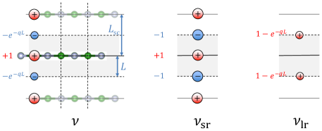
Figure 8: Interpretation of the Coulomb truncation technique as an image-charge method, and its separation into long-range and short-range contributions. The shaded areas refer to the region of space where the three kernels exactly match those illustrated in Fig. 2.

The implementation of the Coulomb cutoff technique follows the prescriptions of Refs. Ismail-Beigi, 2006; Sohier et al., 2016, 2017b, and consists in writing the open-boundary Coulomb kernel as

$$\nu({\bf K_{\parallel}},G_{n})=\frac{4\pi}{K_{\parallel}^{2}+G_{n}^{2}}\left[1-e^{-K_{\parallel}L}\cos(G_{n}L)\right],$$ (73)

where ${\bf K_{\parallel}}={\bf G}_{\parallel}+{\bf q}$ is an in-plane reciprocal-space vector (${\bf G}_{\parallel}$ spans the Bravais lattice of the primitive 2D cell); $G_{n}$ form a discrete mesh along $z$ and $L=L_{\rm sc}/2$ is set to half the supercell length in the out-of-plane direction. After observing that $G_{n}=\frac{\pi n}{L}$, we immediately obtain the following expression for the macroscopic ${\bf G}_{\parallel}=0$ component,

$$\nu({\bf q},G_{n})=\frac{4\pi}{q^{2}+G_{n}^{2}}[1-(-1)^{n}e^{-qL}].$$ (74)

To link these expressions to the arguments of Section II.3, we shall rewrite the prefactor in the square brackets as follows,

$$[1-(-1)^{n}e^{-qL}]=[1-(-1)^{n}]+(-1)^{n}(1-e^{-qL})$$ (75)

It is easy to see that the first term on the rhs corresponds to the short-range “zone-boundary” electrostatics,

$$\nu_{\rm sr}({\bf q},G_{n})=\frac{4\pi}{q^{2}+G_{n}^{2}}[1-(-1)^{n}].$$ (76)

Indeed, the $[1-(-1)^{n}]$ prefactor can be regarded as an implementation of the image-charge method illustrated in Fig. 2. (That this kernel is short-ranged is obvious from Eq. (76): even values of the out-of-plane index $n$ are suppressed, thus excluding the problematic $n=0$ term.) This latter observation reveals that the Coulomb cutoff technique can also be interpreted as an image-charge method: it only differs from $\nu_{\rm sr}$ in the prefactor $e^{-qL}$ that scales the negative images, located at odd multiples of $L$ from the $z=0$ plane. Then, we identify the long-range part of the kernel with the remainder,

$$\nu_{\rm lr}({\bf q},G_{n})=4\pi\frac{(-1)^{n}}{q^{2}+G_{n}^{2}}(1-e^{-qL}).$$ (77)

To verify that Eq. (77) is consistent with the formalism of the earlier sections, recall the following relation for the Fourier series of the hyperbolic cosine function,

$$\int_{-\pi}^{\pi}\cosh(ax)\cos(nx)dx=(-1)^{n}\frac{2a\sinh(a\pi)}{a^{2}+n^{2}}.$$ (78)

By changing the variable to $z=Lx/\pi$, and by setting $q=\frac{a\pi}{L}$, we have

$$\int_{-L}^{L}\cosh(qz)\cos(G_{n}z)dz=(-1)^{n}\frac{2q\sinh(qL)}{q^{2}+G_{n}^{2}}.$$ (79)

Then, observe that

$$\sinh(qL)\left[1-\tanh\left(\frac{qL}{2}\right)\right]=(1-e^{-qL}).$$ (80)

By combining the above, we eventually obtain

$$\int_{-L}^{L}\nu_{\rm lr}({\bf q},z)e^{iG_{n}z}dz=\nu_{\rm lr}({\bf q},G_{n}),$$ (81)

with $\nu_{\rm lr}({\bf q},z)$ defined as in Eq. (35). The above formulas provide, therefore, the desired representation of the short-range and long-range Coulomb kernels in a supercell context, together with an explicit reciprocal-space expression, Eq. (79), for the hyperbolic cosine potential of Eq. (37), which can be directly implemented in a first-principles code. (Similar formulas can be easily derived for the mirror-odd component.)

Appendix D Hyperbolic functions and traceless multipoles

We shall provide a formal demonstration of our statement in Sec.II.5, that the hyperbolic functions consistently pick the traceless component of the first-order charge perturbation at any order in ${\bf q}$. To that end, we shall assume without loss of generality that the $x$ Cartesian axis is aligned with the propagation vector, ${\bf q}=(q,0,0)$, and write the cell-periodic part of the external charge density perturbation, $\rho^{\rm sr,\bf q}_{\kappa\alpha}({\bf r})$, as a lattice sum of the charge densities that are induced by a displacement of isolated atom,

$$\rho^{\rm sr,\bf q}_{\kappa\alpha}({\bf r})=e^{-iqx}\sum_{l}\rho^{\rm sr}_{\kappa\alpha}({\bf r}-{\bf R}_{l\kappa})e^{iqX_{l\kappa}}.$$ (82)

The small-space representation of the charge response, $\tilde{\rho}^{\rm sr}$, then reads

$$\begin{split}\rho^{{\rm sr},(l)}(q)=&\frac{1}{S}\int_{\rm cell}dxdy\int dze^{-iq(x-X_{l\kappa)}}\varphi_{l}(z)\rho^{\rm sr}_{\kappa\alpha}({\bf r}-{\bf R}_{l\kappa})\\ =&\frac{1}{S}\int d^{3}re^{-iqx}\varphi_{l}(z)\rho^{\rm sr}_{\kappa\alpha}({\bf r}),\end{split}$$ (83)

where the integral in the second line is taken over all space, and the origin is set at the projection of the atom $\kappa$ of the $l=0$ cell on the $z=0$ plane, $(X_{0\kappa},Y_{0\kappa},0)$. [Following the notation of the main text, $\varphi_{l}(z)$ stands for the hyperbolic cosine ($l=\parallel$) or sine ($l=\perp$).]

	0	1	2	3
cosh ($\parallel$)	1	$-ix$	$-x^{2}+z^{2}$	$ix^{3}-3ixz^{2}$
sinh ($\perp$)	0	$z$	$-2ixz$	$3xz^{2}-z^{3}$

Table 3: Multipolar expansion of the basis functions $F^{\parallel,\perp}_{n}(x,z)$ in Cartesian coordinates. The columns correspond to $n$.

The function in the integrand can be written as follows,

$$e^{-iqx}\varphi_{l}(z)=\frac{e^{q(-ix+z)}\pm e^{q(-ix-z)}}{2},$$ (84)

where the plus and minus sign refer to cosine and sine, respectively. The expansion of the exponential in powers of $q$ trivially leads to

$$e^{q(-ix+z)}\simeq 1+q(-ix+z)+\frac{q^{2}}{2!}(-ix+z)^{2}+\cdots$$ (85)

If we write the complex number in the round brackets in terms of its modulus, $r$, times a unitary phase, $e^{i\phi}$, we arrive at

$$e^{q(-ix+z)}=\sum_{n=0}^{\infty}\frac{q^{n}}{n!}r^{n}e^{in\phi}.$$ (86)

One can easily recognize the solutions of the Laplace equation in cylindrical coordinates, given by the $n$-th power of the radial coordinate $r$ times a cylindrical harmonic of the same order,

$$F_{n}(r,\phi)=r^{n}e^{in\phi}.$$ (87)

For any $n>0$, there are two (and only two) linearly independent solutions, which we can write as

$$F^{\parallel,\perp}_{n}(r,\phi)=\frac{F_{n}(r,\phi)\pm F_{n}(r,-\phi)}{2}.$$ (88)

(We have taken their mirror-even and mirror-odd linear combinations with respect to $z$-reflection.) Finally, we have

$$e^{-iqx}\varphi_{\parallel,\perp}(z)=\sum_{n=0}^{\infty}\frac{q^{n}}{n!}F^{\parallel,\perp}_{n}(r,\phi).$$ (89)

This shows that the cosh and sinh basis functions correspond to the 2D Fourier transforms of $F^{\parallel,\perp}_{n}$; it is easy to show that $e^{iqx}\varphi_{l}(z)$ are themselves solution of the Laplace equation in two dimensions.

Based on the above, we can conclude that, at any given order $n>0$, there are two (and only two) independent multipolar component of the bounded charge distribution $\rho^{\rm sr}_{\kappa\alpha}({\bf r})$ that produce long-range electrostatic potentials; these are given by the integrals

$$M^{\parallel,\perp}_{\kappa\alpha}(n)=\frac{1}{S}\int d^{3}rF^{\parallel,\perp}_{n}(x,z)\rho^{\rm sr}_{\kappa\alpha}({\bf r}).$$ (90)

From Eq. (84) it is easy to work out a Cartesian representation for the lowest orders, which we report in Table 3. This shows that the individual components of the Cartesian multipole tensors [which are defined by replacing $F^{\parallel,\perp}_{n}(x,z)$ with $x^{j}z^{k}$ in Eq. (90)] are not necessarily relevant for the long-range electrostatics – only their linear combinations, taken according to the prescriptions of Table 3, are. These linear combinations result in removing the trace of the Cartesian tensors at any given order $j+k$ – this is obvious in the $n=2$ case, where the mirror-even quadrupole is given by the difference of the (diagonal) $x^{2}$ and $z^{2}$ components. This is nicely consistent with Eq. (44).

References

- Born and Huang (1954) Max Born and Kun Huang, Dynamical Theory of Crystal Lattices (Oxford University Press, Oxford, 1954).
- Cochran and Cowley (1962) W. Cochran and R.A. Cowley, “Dielectric constants and lattice vibrations,” Journal of Physics and Chemistry of Solids 23, 447–450 (1962).
- Pick et al. (1970) Robert M. Pick, Morrel H. Cohen, and Richard M. Martin, “Microscopic theory of force constants in the adiabatic approximation,” Phys. Rev. B 1, 910–920 (1970).
- Zein (1984) NE Zein, “Density functional calculations of crystal elastic modula and phonon-spectra,” Fiz. Tverd. Tela 26, 3028–3034 (1984).
- Baroni et al. (1987) Stefano Baroni, Paolo Giannozzi, and Andrea Testa, “Green’s-function approach to linear response in solids,” Phys. Rev. Lett. 58, 1861–1864 (1987).
- Gonze (1995a) Xavier Gonze, “Perturbation expansion of variational principles at arbitrary order,” Phys. Rev. A 52, 1086–1095 (1995a).
- Gonze (1995b) Xavier Gonze, “Adiabatic density-functional perturbation theory,” Phys. Rev. A 52, 1096–1114 (1995b).
- Gonze (1997) Xavier Gonze, “First-principles responses of solids to atomic displacements and homogeneous electric fields: Implementation of a conjugate-gradient algorithm,” Phys. Rev. B 55, 10337–10354 (1997).
- Gonze and Lee (1997a) X. Gonze and C. Lee, “Dynamical matrices, Born effective charges, dielectric permittivity tensors, and interatomic force constants from density-functional perturbation theory,” Phys. Rev. B 55, 10355 (1997a).
- Baroni et al. (2001) S. Baroni, S. de Gironcoli, and A. Dal Corso, “Phonons and related crystal properties from density-functional perturbation theory,” Rev. Mod. Phys. 73, 515 (2001).
- Stengel (2013a) M. Stengel, “Flexoelectricity from density-functional perturbation theory,” Phys. Rev. B 88, 174106 (2013a).
- Royo et al. (2020) Miquel Royo, Konstanze R. Hahn, and Massimiliano Stengel, “Using high multipolar orders to reconstruct the sound velocity in piezoelectrics from lattice dynamics,” Phys. Rev. Lett. 125, 217602 (2020).
- Ismail-Beigi (2006) Sohrab Ismail-Beigi, “Truncation of periodic image interactions for confined systems,” Phys. Rev. B 73, 233103 (2006).
- Rozzi et al. (2006) Carlo A. Rozzi, Daniele Varsano, Andrea Marini, Eberhard K. U. Gross, and Angel Rubio, “Exact Coulomb cutoff technique for supercell calculations,” Phys. Rev. B 73, 205119 (2006).
- Sohier et al. (2017a) Thibault Sohier, Marco Gibertini, Matteo Calandra, Francesco Mauri, and Nicola Marzari, “Breakdown of optical phonons splitting in two-dimensional materials,” Nano Letters 17, 3758–3763 (2017a).
- Luca et al. (2020) Marta De Luca, Xavier Cartoixà, David I Indolese, Javier Martín-Sánchez, Kenji Watanabe, Takashi Taniguchi, Christian Schönenberger, Rinaldo Trotta, Riccardo Rurali, and Ilaria Zardo, “Experimental demonstration of the suppression of optical phonon splitting in 2D materials by Raman spectroscopy,” 2D Materials 7, 035017 (2020).
- Sánchez-Portal and Hernández (2002) D. Sánchez-Portal and E. Hernández, “Vibrational properties of single-wall nanotubes and monolayers of hexagonal BN,” Phys. Rev. B 66, 235415 (2002).
- Michel and Verberck (2011) K. H. Michel and B. Verberck, “Phonon dispersions and piezoelectricity in bulk and multilayers of hexagonal boron nitride,” Phys. Rev. B 83, 115328 (2011).
- Sohier et al. (2016) Thibault Sohier, Matteo Calandra, and Francesco Mauri, “Two-dimensional Fröhlich interaction in transition-metal dichalcogenide monolayers: Theoretical modeling and first-principles calculations,” Phys. Rev. B 94, 085415 (2016).
- Sohier et al. (2018) Thibault Sohier, Davide Campi, Nicola Marzari, and Marco Gibertini, “Mobility of two-dimensional materials from first principles in an accurate and automated framework,” Phys. Rev. Materials 2, 114010 (2018).
- Li et al. (2019) Wenbin Li, Samuel Poncé, and Feliciano Giustino, “Dimensional crossover in the carrier mobility of two-dimensional semiconductors: The case of InSe,” Nano Letters 19, 1774–1781 (2019).
- Ma et al. (2020) Jinlong Ma, Dongwei Xu, Run Hu, and Xiaobing Luo, “Examining two-dimensional Fröhlich model and enhancing the electron mobility of monolayer InSe by dielectric engineering,” Journal of Applied Physics 128, 035107 (2020).
- Poncé et al. (2020) Samuel Poncé, Wenbin Li, Sven Reichardt, and Feliciano Giustino, “First-principles calculations of charge carrier mobility and conductivity in bulk semiconductors and two-dimensional materials,” Reports on Progress in Physics 83, 036501 (2020).
- Deng et al. (2021) Tianqi Deng, Gang Wu, Wen Shi, Zicong Marvin Wong, Jian-Sheng Wang, and Shuo-Wang Yang, “Ab initio dipolar electron-phonon interactions in two-dimensional materials,” Phys. Rev. B 103 (2021), 10.1103/physrevb.103.075410.
- Andersen et al. (2015) Kirsten Andersen, Simone Latini, and Kristian S. Thygesen, “Dielectric genome of van der waals heterostructures,” Nano Lett. 15, 4616–4621 (2015).
- Mohn et al. (2018) Michael J. Mohn, Ralf Hambach, Philipp Wachsmuth, Christine Giorgetti, and Ute Kaiser, “Dielectric properties of graphene/ mos2 heterostructures from ab initio calculations and electron energy-loss experiments,” Phys. Rev. B 97 (2018), 10.1103/physrevb.97.235410.
- Sohier et al. (2021) Thibault Sohier, Marco Gibertini, and Matthieu J. Verstraete, “Remote free-carrier screening to boost the mobility of fröhlich-limited two-dimensional semiconductors,” Phys. Rev. Materials 5 (2021), 10.1103/physrevmaterials.5.024004.
- Sponza and Ducastelle (2020) Lorenzo Sponza and François Ducastelle, “Proper ab-initio dielectric function of 2d materials and their polarizable thickness,” arXiv preprint arXiv:2011.07811 (2020).
- Stengel (2013b) M. Stengel, “Microscopic response to inhomogeneous deformations in curvilinear coordinates,” Nature Communications 4, 2693 (2013b).
- Stengel and Vanderbilt (2016) Massimiliano Stengel and David Vanderbilt, “First-principles theory of flexoelectricity,” in Flexoelectricity in Solids From Theory to Applications, edited by Alexander K. Tagantsev and Petr V. Yudin (World Scientific Publishing Co., Singapore, 2016) Chap. 2, pp. 31–110.
- Royo and Stengel (2019) Miquel Royo and Massimiliano Stengel, “First-principles theory of spatial dispersion: Dynamical quadrupoles and flexoelectricity,” Phys. Rev. X 9, 021050 (2019).
- Springolo et al. (2020) Matteo Springolo, Miquel Royo, and Massimiliano Stengel, “Flexoelectricity in two-dimensional materials,” arXiv preprint arXiv:2010.08470 (2020).
- Ando et al. (1982) Tsuneya Ando, Alan B. Fowler, and Frank Stern, “Electronic properties of two-dimensional systems,” Rev. Mod. Phys. 54, 437–672 (1982).
- Kotov et al. (2012) Valeri N. Kotov, Bruno Uchoa, Vitor M. Pereira, F. Guinea, and A. H. Castro Neto, “Electron-electron interactions in graphene: Current status and perspectives,” Rev. Mod. Phys. 84, 1067–1125 (2012).
- Freysoldt et al. (2008) Christoph Freysoldt, Philipp Eggert, Patrick Rinke, Arno Schindlmayr, and Matthias Scheffler, “Screening in two dimensions: calculations for surfaces and thin films using the repeated-slab approach,” Phys. Rev. B 77, 235428 (2008).
- Cudazzo et al. (2011) Pierluigi Cudazzo, Ilya V. Tokatly, and Angel Rubio, “Dielectric screening in two-dimensional insulators: Implications for excitonic and impurity states in graphane,” Phys. Rev. B 84, 085406 (2011).
- Berkelbach et al. (2013) Timothy C. Berkelbach, Mark S. Hybertsen, and David R. Reichman, “Theory of neutral and charged excitons in monolayer transition metal dichalcogenides,” Phys. Rev. B 88, 045318 (2013).
- Latini et al. (2015) S. Latini, T. Olsen, and K. S. Thygesen, “Excitons in van der waals heterostructures: The important role of dielectric screening,” Phys. Rev. B 92, 245123 (2015).
- Kylänpää and Komsa (2015) Ilkka Kylänpää and Hannu-Pekka Komsa, “Binding energies of exciton complexes in transition metal dichalcogenide monolayers and effect of dielectric environment,” Phys. Rev. B 92, 205418 (2015).
- Hüser et al. (2013) Falco Hüser, Thomas Olsen, and Kristian S. Thygesen, “How dielectric screening in two-dimensional crystals affects the convergence of excited-state calculations: Monolayer MoS2,” Phys. Rev. B 88, 245309 (2013).
- Yan et al. (2011) Jun Yan, Kristian S. Thygesen, and Karsten W. Jacobsen, “Nonlocal screening of plasmons in graphene by semiconducting and metallic substrates: First-principles calculations,” Phys. Rev. Lett. 106, 146803 (2011).
- Andersen et al. (2014) Kirsten Andersen, Karsten W. Jacobsen, and Kristian S. Thygesen, “Plasmons on the edge of nanostructures,” Phys. Rev. B 90, 161410 (2014).
- Ghosh et al. (2017) Barun Ghosh, Piyush Kumar, Anmol Thakur, Yogesh Singh Chauhan, Somnath Bhowmick, and Amit Agarwal, “Anisotropic plasmons, excitons, and electron energy loss spectroscopy of phosphorene,” Phys. Rev. B 96, 035422 (2017).
- Agarwal et al. (2018) Amit Agarwal, Miriam S Vitiello, Leonardo Viti, Anna Cupolillo, and Antonio Politano, “Plasmonics with two-dimensional semiconductors: from basic research to technological applications,” Nanoscale 10, 8938–8946 (2018).
- Trolle et al. (2017) Mads L. Trolle, Thomas G. Pedersen, and Valerie Véniard, “Model dielectric function for 2D semiconductors including substrate screening,” Scientific Reports 7, 39844 (2017).
- Martin et al. (2016) Richard M Martin, Lucia Reining, and David M Ceperley, Interacting electrons (Cambridge University Press, Cambridge, United Kingdom, 2016).
- Gonze and Lee (1997b) X. Gonze and C. Lee, “Dynamical matrices, Born effective charges, dielectric permittivity tensors, and interatomic force constants from density-functional perturbation theory,” Phys. Rev. B 55, 10355 (1997b).
- Giannozzi et al. (2009) Paolo Giannozzi, Stefano Baroni, Nicola Bonini, Matteo Calandra, Roberto Car, Carlo Cavazzoni, Davide Ceresoli, Guido L Chiarotti, Matteo Cococcioni, Ismaila Dabo, Andrea Dal Corso, Stefano de Gironcoli, Stefano Fabris, Guido Fratesi, Ralph Gebauer, Uwe Gerstmann, Christos Gougoussis, Anton Kokalj, Michele Lazzeri, Layla Martin-Samos, Nicola Marzari, Francesco Mauri, Riccardo Mazzarello, Stefano Paolini, Alfredo Pasquarello, Lorenzo Paulatto, Carlo Sbraccia, Sandro Scandolo, Gabriele Sclauzero, Ari P Seitsonen, Alexander Smogunov, Paolo Umari, and Renata M Wentzcovitch, “QUANTUM ESPRESSO: a modular and open-source software project for quantum simulations of materials,” Journal of Physics: Condensed Matter 21, 395502 (2009).
- Gonze et al. (2009) X. Gonze, B. Amadon, P.-M. Anglade, J.-M. Beuken, F. Bottin, P. Boulanger, F. Bruneval, D. Caliste, R. Caracas, M. Côté, T. Deutsch, L. Genovese, Ph. Ghosez, M. Giantomassi, S. Goedecker, D.R. Hamann, P. Hermet, F. Jollet, G. Jomard, S. Leroux, M. Mancini, S. Mazevet, M.J.T. Oliveira, G. Onida, Y. Pouillon, T. Rangel, G.-M. Rignanese, D. Sangalli, R. Shaltaf, M. Torrent, M.J. Verstraete, G. Zerah, and J.W. Zwanziger, “ABINIT: First-principles approach to material and nanosystem properties,” Computer Phys. Commun. 180, 2582–2615 (2009).
- Sohier et al. (2017b) Thibault Sohier, Matteo Calandra, and Francesco Mauri, “Density functional perturbation theory for gated two-dimensional heterostructures: Theoretical developments and application to flexural phonons in graphene,” Phys. Rev. B 96, 075448 (2017b).
- Applequist (1989) J Applequist, “Traceless cartesian tensor forms for spherical harmonic functions: new theorems and applications to electrostatics of dielectric media,” J. Phys. A: Math. Gen. 22, 4303–4330 (1989).
- Zubko et al. (2016) Pavlo Zubko, Jacek C Wojdeł, Marios Hadjimichael, Stéphanie Fernandez-Pena, Anaïs Sené, Igor Luk’yanchuk, Jean-Marc Triscone, and Jorge Íñiguez, “Negative capacitance in multidomain ferroelectric superlattices,” Nature 534, 524–528 (2016).
- Junquera et al. (2007) J. Junquera, M. H. Cohen, and K. M. Rabe, “Nanoscale smoothing and the analyis of interfacial charge and dipolar densities,” J. Phys.: Condens. Matter 19, 213203 (2007).
- Baldereschi et al. (1988) A. Baldereschi, S. Baroni, and R. Resta, “Band offsets in lattice-matched heterojunctions: a model and first-principles calculations for GaAs/AlAs,” Phys. Rev. Lett. 61, 734–737 (1988).
- Martin (1972) Richard M. Martin, “Piezoelectricity,” Phys. Rev. B 5, 1607–1613 (1972).
- Romero et al. (2020) Aldo H. Romero, Douglas C. Allan, Bernard Amadon, Gabriel Antonius, Thomas Applencourt, Lucas Baguet, Jordan Bieder, François Bottin, Johann Bouchet, Eric Bousquet, Fabien Bruneval, Guillaume Brunin, Damien Caliste, Michel Côté, Jules Denier, Cyrus Dreyer, Philippe Ghosez, Matteo Giantomassi, Yannick Gillet, Olivier Gingras, Donald R. Hamann, Geoffroy Hautier, François Jollet, Gérald Jomard, Alexandre Martin, Henrique P. C. Miranda, Francesco Naccarato, Guido Petretto, Nicholas A. Pike, Valentin Planes, Sergei Prokhorenko, Tonatiuh Rangel, Fabio Ricci, Gian-Marco Rignanese, Miquel Royo, Massimiliano Stengel, Marc Torrent, Michiel J. van Setten, Benoit Van Troeye, Matthieu J. Verstraete, Julia Wiktor, Josef W. Zwanziger, and Xavier Gonze, “ABINIT: Overview and focus on selected capabilities,” The Journal of Chemical Physics 152, 124102 (2020).
- Hamann (2013) D. R. Hamann, “Optimized norm-conserving Vanderbilt pseudopotentials,” Phys. Rev. B 88, 085117 (2013).
- van Setten et al. (2018) M.J. van Setten, M. Giantomassi, E. Bousquet, M.J. Verstraete, D.R. Hamann, X. Gonze, and G.-M. Rignanese, “The PseudoDojo: Training and grading a 85 element optimized norm-conserving pseudopotential table,” Computer Physics Communications 226, 39–54 (2018).
- Giannozzi et al. (2017) P Giannozzi, O Andreussi, T Brumme, O Bunau, M Buongiorno Nardelli, M Calandra, R Car, C Cavazzoni, D Ceresoli, M Cococcioni, N Colonna, I Carnimeo, A Dal Corso, S de Gironcoli, P Delugas, R A DiStasio, A Ferretti, A Floris, G Fratesi, G Fugallo, R Gebauer, U Gerstmann, F Giustino, T Gorni, J Jia, M Kawamura, H-Y Ko, A Kokalj, E Küçükbenli, M Lazzeri, M Marsili, N Marzari, F Mauri, N L Nguyen, H-V Nguyen, A Otero de-la Roza, L Paulatto, S Poncé, D Rocca, R Sabatini, B Santra, M Schlipf, A P Seitsonen, A Smogunov, I Timrov, T Thonhauser, P Umari, N Vast, X Wu, and S Baroni, “Advanced capabilities for materials modelling with quantum ESPRESSO,” Journal of Physics: Condensed Matter 29, 465901 (2017).
- Jiang et al. (2018) Jin-Wu Jiang, Bing-Shen Wang, and Harold S. Park, “Topologically protected interface phonons in two-dimensional nanomaterials: hexagonal boron nitride and silicon carbide,” Nanoscale 10, 13913–13923 (2018).
- Wirtz et al. (2003) Ludger Wirtz, Angel Rubio, Raul Arenal de la Concha, and Annick Loiseau, “Ab initio calculations of the lattice dynamics of boron nitride nanotubes,” Phys. Rev. B 68, 045425 (2003).
- Zhen and Wang (2020) Zhi-Qiang Zhen and Hai-Yan Wang, “Density functional study of the electronic, elastic, and lattice dynamic properties of SnS2,” Acta Physica Polonica, A. 137 (2020).
- Shafique et al. (2017) Aamir Shafique, Abdus Samad, and Young-Han Shin, “Ultra low lattice thermal conductivity and high carrier mobility of monolayer SnS2 and SnSe2: a first principles study,” Physical Chemistry Chemical Physics 19, 20677–20683 (2017).
- He et al. (2018) Wenke He, Dongyang Wang, Jin-Feng Dong, Yang Qiu, Liangwei Fu, Yue Feng, Yujie Hao, Guangtao Wang, Jinfeng Wang, Chang Liu, et al., “Remarkable electron and phonon band structures lead to a high thermoelectric performance in earth-abundant and eco-friendly SnS crystals,” Journal of Materials Chemistry A 6, 10048–10056 (2018).
- Di Lu et al. (2016) Di Lu, David J Baek, Seung Sae Hong, Lena F Kourkoutis, Yasuyuki Hikita, and Harold Y Hwang, “Synthesis of freestanding single-crystal perovskite films and heterostructures by etching of sacrificial water-soluble layers,” Nature Materials 15, 1255–1260 (2016).
- Hong et al. (2020) Seung Sae Hong, Mingqiang Gu, Manish Verma, Varun Harbola, Bai Yang Wang, Di Lu, Arturas Vailionis, Yasuyuki Hikita, Rossitza Pentcheva, James M. Rondinelli, and Harold Y. Hwang, “Extreme tensile strain states in La0.7Ca0.3MnO3 membranes,” Science 368, 71–76 (2020).
- Brunin et al. (2020a) Guillaume Brunin, Henrique Pereira Coutada Miranda, Matteo Giantomassi, Miquel Royo, Massimiliano Stengel, Matthieu J. Verstraete, Xavier Gonze, Gian-Marco Rignanese, and Geoffroy Hautier, “Electron-phonon beyond Fröhlich: Dynamical quadrupoles in polar and covalent solids,” Phys. Rev. Lett. 125, 136601 (2020a).
- Brunin et al. (2020b) Guillaume Brunin, Henrique Pereira Coutada Miranda, Matteo Giantomassi, Miquel Royo, Massimiliano Stengel, Matthieu J. Verstraete, Xavier Gonze, Gian-Marco Rignanese, and Geoffroy Hautier, “Phonon-limited electron mobility in Si, GaAs, and GaP with exact treatment of dynamical quadrupoles,” Phys. Rev. B 102, 094308 (2020b).
- Jhalani et al. (2020) Vatsal A. Jhalani, Jin-Jian Zhou, Jinsoo Park, Cyrus E. Dreyer, and Marco Bernardi, “Piezoelectric electron-phonon interaction from ab initio dynamical quadrupoles: Impact on charge transport in wurtzite GaN,” Phys. Rev. Lett. 125, 136602 (2020).
- Park et al. (2020) Jinsoo Park, Jin-Jian Zhou, Vatsal A. Jhalani, Cyrus E. Dreyer, and Marco Bernardi, “Long-range quadrupole electron-phonon interaction from first principles,” Phys. Rev. B 102, 125203 (2020).
- Felipe et al. (2020) H Felipe, Lede Xian, Angel Rubio, and Steven G Louie, “Universal slow plasmons and giant field enhancement in atomically thin quasi-two-dimensional metals,” Nature communications 11, 1–10 (2020).
- Tian et al. (2020) Tian Tian, Declan Scullion, Dale Hughes, Lu Hua Li, Chih-Jen Shih, Jonathan Coleman, Manish Chhowalla, and Elton J. G. Santos, “Electronic polarizability as the fundamental variable in the dielectric properties of two-dimensional materials,” Nano Letters 20, 841–851 (2020).