Autocomplete Element Pattern Design

Autocomplete Zentangle Design

Autocomplete Pattern Design

Autocomplete Pattern Design with Interactive Learning

Autocomplete Hierarchical Pattern Design with Interactive Learning

Autocomplete Complex Hierarchical Pattern Design with Online Parameter Learning

Autocomplete Hierarchical Pattern Design via Online Parameter Learning

Brushing Continuous Vector Patterns

Synthesizing Continuous Patterns from User Exemplars

Continuous Curve Textures

Abstract.

Repetitive patterns are ubiquitous in natural and human-made objects, and can be created with a variety of tools and methods. Manual authoring provides unmatched degree of freedom and control, but can require significant artistic expertise and manual labor. Computational methods can automate parts of the manual creation process, but are mainly tailored for discrete pixels or elements instead of more general continuous structures. We propose an example-based method to synthesize continuous curve patterns from exemplars. Our main idea is to extend prior sample-based discrete element synthesis methods to consider not only sample positions (geometry) but also their connections (topology). Since continuous structures can exhibit higher complexity than discrete elements, we also propose robust, hierarchical synthesis to enhance output quality. Our algorithm can generate a variety of continuous curve patterns fully automatically. For further quality improvement and customization, we also present an autocomplete user interface to facilitate interactive creation and iterative editing. We evaluate our methods and interface via different patterns, ablation studies, and comparisons with alternative methods.

(a) Output of LABEL:sub@fig:teaser:string:input

(b) String

(c) Strip

(d) Output of LABEL:sub@fig:teaser:strip:input

(e) Output of LABEL:sub@fig:teaser:maze:input

(f) Maze

(g) Branches

(h) Output of LABEL:sub@fig:teaser:branch:input

Figure 1. Example inputs and outputs of our method. Given a small input exemplar, our algorithm can synthesize various types of continuous curve textures. Our results are shown in vector format. Please zoom in to see the details.

1. Introduction

(a) Exemplar

(b) Samples of LABEL:sub@fig:comparison_sample_synthesis:exemplar

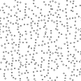
(c) [Ma et al., 2011]

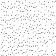
(d) [Roveri et al., 2015]

(e) [Tu et al., 2019]

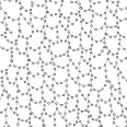
(f) Our output samples

(g) Reconstruction of LABEL:sub@fig:comparison_sample_synthesis:ours:sample_synthesis

Figure 2. Comparison with prior point/sample synthesis algorithms. The methods in [Ma et al., 2011; Roveri et al., 2015; Tu et al., 2019] generate samples without considering their connections in the exemplars LABEL:sub@fig:comparison_sample_synthesis:exemplar_samples. Thus, their results, as shown in LABEL:sub@fig:comparison_sample_synthesis:ma, LABEL:sub@fig:comparison_sample_synthesis:roveri, and LABEL:sub@fig:comparison_sample_synthesis:tu, preserve the sample distributions less well than ours in LABEL:sub@fig:comparison_sample_synthesis:ours:sample_synthesis. It is also unclear how to reconstruct continuous curve patterns from LABEL:sub@fig:comparison_sample_synthesis:ma, LABEL:sub@fig:comparison_sample_synthesis:roveri, and LABEL:sub@fig:comparison_sample_synthesis:tu. LABEL:sub@fig:comparison_sample_synthesis:ours:curve_recon shows the curve reconstruction from LABEL:sub@fig:comparison_sample_synthesis:ours:sample_synthesis.

Repetitive patterns are fundamental for a variety of tasks in design [Kazi et al., 2012; Lu et al., 2014] and engineering [Zhou et al., 2014; Martínez et al., 2015; Zehnder et al., 2016; Chen et al., 2016; Schumacher et al., 2016]. Manually creating these patterns provides high degrees of individual freedom, but can also require significant technical/artistic expertise and manual labor. These usability barriers can be reduced by automatic methods that can synthesize patterns similar to user-supplied exemplars [Ma et al., 2011; Ma et al., 2013; Ijiri et al., 2008; Hurtut et al., 2009; Barla et al., 2006; Kazi et al., 2012; Lu et al., 2014; Suzuki et al., 2017; Hsu et al., 2018, 2020]. However, existing techniques mainly focus on discrete patterns consisting of image pixels or shape elements, and might not apply to general patterns consisting of continuous curves, which can be connected or intersected with one another.

We propose an example-based method that can automatically synthesize continuous curve patterns from user-supplied exemplars. Similar to prior pixel/sample-based methods [Wei et al., 2009; Ma et al., 2011; Lu et al., 2012; Landes et al., 2013; Ma et al., 2013; Lu et al., 2014; Roveri et al., 2015], users can provide exemplars and have the algorithm automatically produce results in desired sizes and shapes. However, different from previous methods and systems that are restricted to discrete pixels/elements or limited continuous structures, our method can handle both discrete elements and continuous curves in a variety of patterns (Figure 1).

Our main idea is to extend prior sample-based element synthesis methods [Ma et al., 2011; Kazi et al., 2012; Ma et al., 2013; Hsu et al., 2018] to consider not only sample positions (geometry) but also their connections (topology) in all major algorithm components, including pattern representation, neighborhood similarity, and synthesis optimization consisting of search and assignment steps. Our algorithm uses a graph representation for both topology synthesis and geometric path reconstruction for general continuous patterns, in contrast to the graph representations in [Hsu et al., 2018, 2020] that only apply to discrete elements. Since continuous patterns can exhibit higher complexity than discrete elements, we propose robust, hierarchical synthesis [Wei and Levoy, 2000, 2001] to enhance output quality.

Automatically generated outputs, although convenient, might not have sufficient quality or fit what users have in mind for their particular applications. To facilitate further editing and customization, we also propose an interactive autocomplete authoring interface [Xing et al., 2014; Hsu et al., 2020] built upon our synthesis algorithm components. Similar to existing design tools, users can create various free-style patterns. When they have sufficient exemplars and would like to reduce further manual repetitions, they can specify an output domain to be automatically filled [Kazi et al., 2012; Xing et al., 2014]. The synthesized patterns resemble and seamlessly connect with what has already been drawn. If not satisfied, users can accept or modify the predictions, or ask for re-synthesis to maintain full control. They can further designate specific source regions for cloning to target regions.

We analyze our algorithm via ablation studies, compare it with alternative methods, and demonstrate the quality and accessibility of our system via pattern design results. We plan to share our code along with the publication of this paper to facilitate reproduction.

In sum, the contributions of this work are:

• A hierarchical representation and a synthesis method for both geometry and topology of continuous and discrete patterns.

• An interactive authoring system with autocomplete functions to reduce manual workloads and facilitate user control.

2. Related Work

Our work is inspired by prior art in vector patterns, image textures, and interactive workflows. Procedural methods [Pedersen and Singh, 2006; Loi et al., 2017; Santoni and Pellacini, 2016] can produce intricate structures, but are limited in scope and difficult to generalize for different types of patterns. Example-based methods are general, but existing work predominantly focuses on image textures [Wei et al., 2009; Lu et al., 2014; Gatys et al., 2016] rather than vector patterns. Below, we survey methods most related to our work.

2.1. Example-based Pattern Generation

Example-based methods are designed to generate large patterns from small exemplars with an optional control provided by the users [Ijiri et al., 2008; Ma et al., 2011; Ma et al., 2013; Hurtut et al., 2009; Barla et al., 2006; Landes et al., 2013; Roveri et al., 2015; Hsu et al., 2018; Tu et al., 2019; Bhat et al., 2004; Zhou et al., 2006; Zhou et al., 2007]. However, these methods target discrete elements or samples [Ijiri et al., 2008; Ma et al., 2011; Hurtut et al., 2009; Landes et al., 2013; Hsu et al., 2018, 2020; Tu et al., 2019] and treat continuous structures as special cases via curve/surface reconstruction from point samples [Ma et al., 2011; Roveri et al., 2015]. Roveri et al. [2015] reconstructs the output surface from synthesized point samples via their associated surface normals without considering sample connections, and thus can only be applied to surfaces relatively smooth to the underlying sampling density. Tu et al. [2019] extends neural point synthesis by treating a graph edge as a line of points, which is essentially point synthesis. The neural optimization method does not provide the same flexibility and efficiency as in our method and it is unstable when the points contain attributes beyond positions. Relatively few works focus on curves, such as enriching details of given coarse curves [Hertzmann et al., 2002] or growing L-system-like curves [Merrell and Manocha, 2010]. Our system is inspired by these prior sample-based algorithms [Ma et al., 2011; Roveri et al., 2015; Hsu et al., 2020], but we explicitly incorporate both samples and their connectivity into our representation and optimization to synthesize more general continuous structures, as shown in Figure 2.

2.2. Interactive Authoring

Workflow analysis has been investigated to assist various content creation task [Nancel and Cockburn, 2014]. Examples includes static and animated sketches [Xing et al., 2014, 2015], 3D sculpting [Peng et al., 2018, 2020], texture design [Suzuki et al., 2017], hand-writing beautification [Zitnick, 2013], and image editing [Chen et al., 2011; Koyama et al., 2016]. Our work is inspired by prior autocomplete [Xing et al., 2014, 2015; Peng et al., 2018; Suzuki et al., 2017] and interactive systems [Kazi et al., 2012; Bian et al., 2018; Hsu et al., 2020]. However, these systems can automate only relatively simple patterns (e.g., repetitive hatches or strokes). Our method can automatically generate diverse and complex continuous curve patterns to facilitate iterative design with reduced input workload.

3. User Interface

Our system can be used for both automatic synthesis and interactive editing. Similar to prior work like traditional texture synthesis [Wei et al., 2009], the user provides an exemplar pattern and lets our system automatically produce the output with desired size and shape. The exemplar is represented via Bézier curves. Inputs in other formats can be converted to Bézier curves (for example, by vectorizing a raster image).

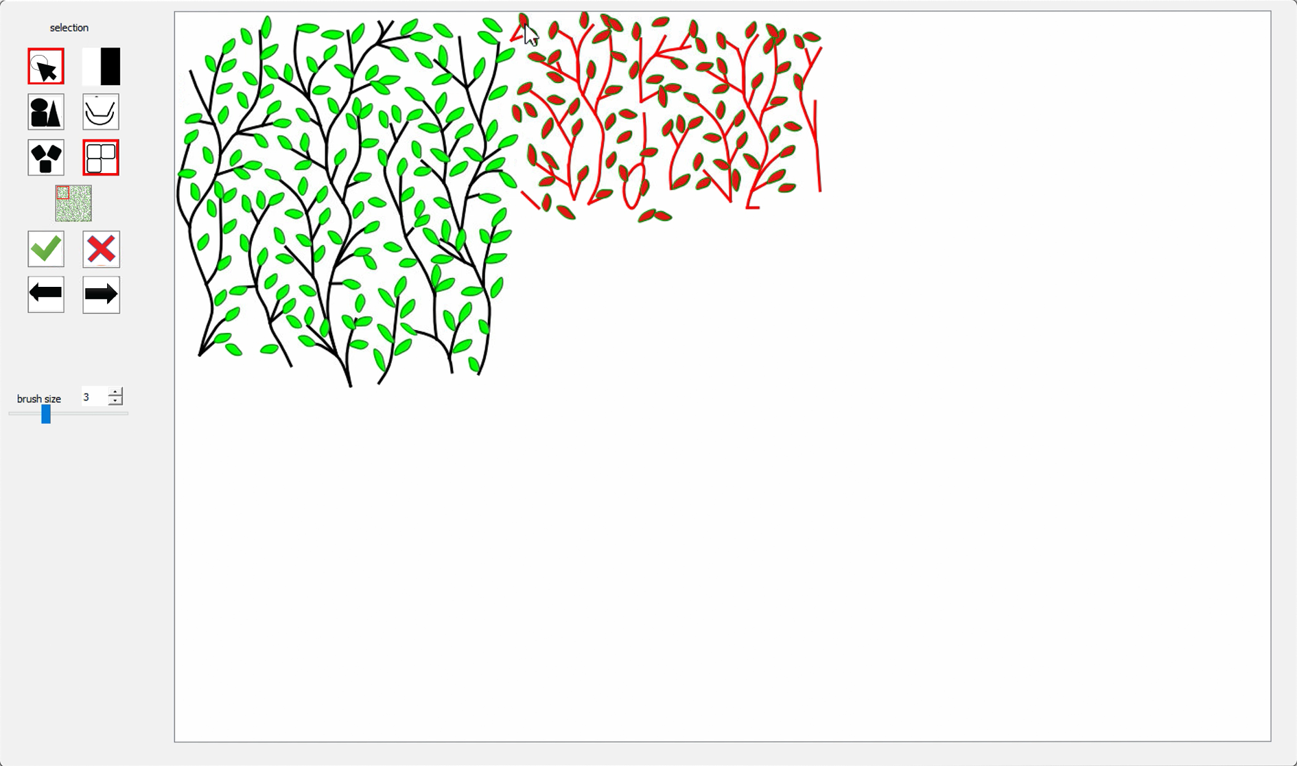
Figure 3. User Interface. Our interface has a widget panel and a canvas. The widget panel provides basic tools, such as selection in a vector editor, as well as controls to the graphics parameters, including color and pen width, and modes unique to our autocomplete system.

Since the automatic synthesis results might not be what the users want and they might need to create new patterns manually, we also provide an interface built upon our automatic synthesis algorithms for users to author patterns interactively. Through the interface, users can specify an output domain in desired size and shape (Figure 4a) and let our system predict patterns that resemble what the users have already drawn (autocomplete mode, Figures 4a and 4b). The users can also explicitly control the prediction by copying-pasting from an input region to an output region (clone mode, Figures 4c and 4d). They can accept, partially accept, or reject the predictions via keyboard shortcuts and mouse selections. They can also perform further edits, such as selecting regions for re-synthesis or adding paths in the predictions. Please refer to the supplementary video for live actions. Since continuous patterns often contain complex structures beyond fine-grained autocomplete of individual strokes [Xing et al., 2014], we design our current interface to focus on autocomplete pattern regions instead of strokes.

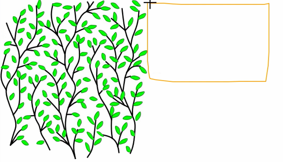
(a) Autocomplete: before

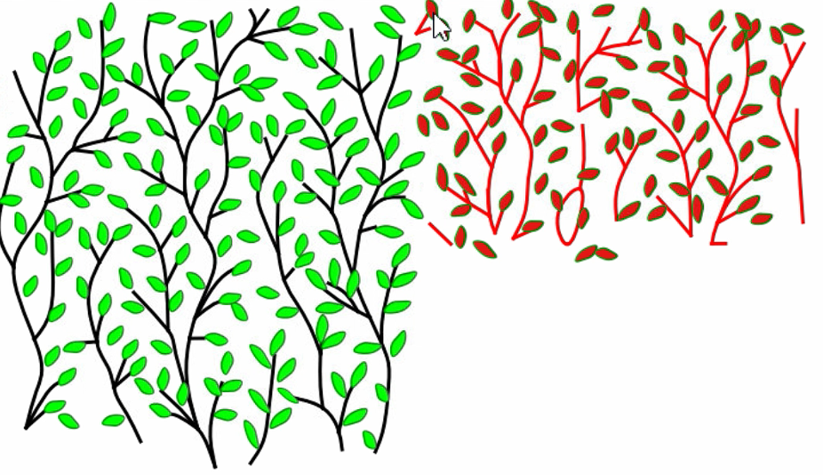
(b) Autocomplete: after

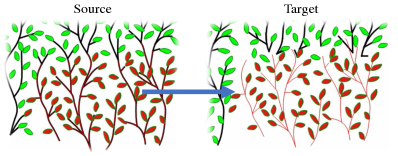
(c) Clone: before

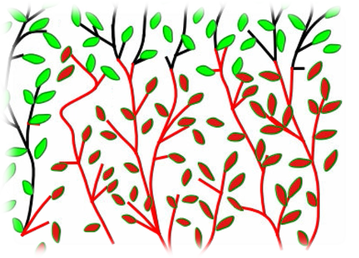
(d) Clone: after

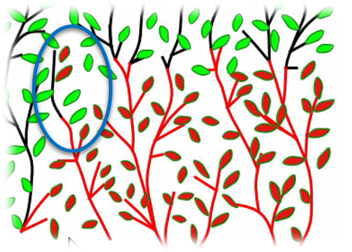
(e) User edit

Figure 4. Autocomplete and clone. In the autocomplete mode, the user can specify an output region (shown in yellow) LABEL:sub@subfig:autocomplete:before and let our system generate predicted patterns LABEL:sub@subfig:autocomplete:after. In the clone mode, the user can specify a source region (in red) and clone it to a target region LABEL:sub@subfig:workflow_clone:before. Our system can generate predictions adaptive to the existing patterns LABEL:sub@subfig:workflow_clone:synthesized, upon which users can perform further refinements LABEL:sub@subfig:user_editing. LABEL:sub@subfig:user_editing is generated by editing the top left corner (in blue) of the predictions, including 1) partially rejecting several paths, 2) copy-pasting two elements, and 3) adding a path.

4. Method

Our method extends the sample-based element texture synthesis method in [Ma et al., 2011] to consider not only individual point samples but also their curved connections via graphs [Hsu et al., 2018, 2020]. We describe our pattern representation in Section 4.1, similarity measures in Section 4.2, and the corresponding synthesis and reconstruction algorithms in Sections 4.3 and 4.4. Our method can handle discrete elements, continuous structures, and their combinations. We will describe when and how our algorithms treat them similarly or differently.

4.1. Representation

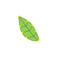
(a) Single-res

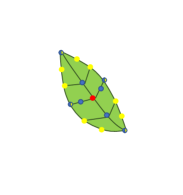
(b) Multi-res

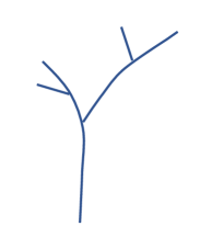
(c) Pattern

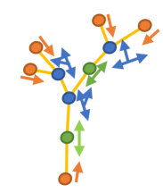
(d) Graph

Figure 5. Pattern representation. Existing algorithms [Ma et al., 2011] only use a single-resolution element representation LABEL:sub@fig:single_resolution_repres. We propose a hierarchical element representation to improve the synthesis quality LABEL:sub@fig:hierarchical_repres. Our synthesis proceeds from red, blue, to yellow samples in coarse to fine levels. A pattern LABEL:sub@fig:continuous_pattern is represented by a graph LABEL:sub@fig:graph_repres, where we record connections (yellow edges) and local path orientations (arrows) in addition to point samples. The color of a sample indicates the number of connections $|\boldsymbol{\mathcal{E}}(s)|$ associated with it; orange, green, and blue indicate 1, 2, and 3.

We represent patterns and elements via point samples and graphs (Figure 5) [Ma et al., 2011; Roveri et al., 2015; Hsu et al., 2018]. Each sample $s$ records its position $\mathbf{p}(s)$, attributes $\mathbf{a}(s)$ (Table 1), and $i(s)\in[0,1]$ to indicate the confidence of its existence to optimize the number of samples:

(1) $$\mathbf{u}(s)=\left(\mathbf{p}(s),\mathbf{a}(s),i(s)\right).$$

Table 1. Sample attributes. Each sample $s$ records its attributes $\mathbf{a}(s)$ that may vary in terms of types of patterns (discrete element or continuous structure). $q(s)\geq 0$ indicates uniqueness of a sample relative to other samples within a discrete element, and $q(s)=-1$ for continuous structures. $\boldsymbol{\mathcal{E}}(s)=\{e_{ss^{\prime}}\}$ records all edges associated with $s$, where $e_{ss^{\prime}}$ is an edge between $s$ and $s^{\prime}$. $\mathbf{o}(s)$ records the local orientations of the paths intersecting at sample $s$.

Attributes	Sample id	Connectivity	Orientation
$\mathbf{a}(s)$	$q(s)$	$\boldsymbol{\mathcal{E}}(s)=\{e_{ss^{\prime}}\}$	$\mathbf{o}(s)$

Discrete elements

Following [Ma et al., 2011; Ma et al., 2013], for discrete elements, sample attributes include a sample id $q(s)$ that indicates the uniqueness of $s$ to other samples within its containing element.

Continuous structures

In discrete element synthesis, it is sufficient to use only samples with id $q(s)$ (Figures 5a and 5b) to encode element shape because every element has the same topology [Ma et al., 2011]. On the other hand, continuous structures are composed of paths and have more flexibilities. In our paper, we represent paths by linear and quadratic Bézier curves, even though other vector curve formats can be easily added. The paths may be connected to each other with complex topologies (Figure 1). Thus, samples alone are not sufficient to disambiguate matching and reconstruction of continuous structures. Therefore, we also consider connectivity among samples, leading to a graph-based representation (Figure 5d). Note the method in [Hsu et al., 2018, 2020] also adopts a graph-based representation, but it is for discrete elements only without explicitly modeling paths in a continuous pattern.

Specifically, we record the connectivity $\boldsymbol{\mathcal{E}}(s)$ for $s$ within $\mathbf{a}(s)$. $\boldsymbol{\mathcal{E}}(s)=\{e_{ss^{\prime}}\}$ is the set of edges associated with $s$, where $e_{ss^{\prime}}$ represents the edge between the two samples $s$ and $s^{\prime}$. We use $i(e)\in[0\ 1]$ to indicate the confidence of an edge existence; $i(e_{ss^{\prime}})=1/0$ indicates the presence/absence of an edge between $s$ and $s^{\prime}$. We will relax the binary $i(e_{ss^{\prime}})$ to be within the range $[0\ 1]$ during optimization-based synthesis. While $\boldsymbol{\mathcal{E}}(s)$ records pattern topology, we also record the tangent angles at $s$ on a path via an orientation attribute $\mathbf{o}\in\mathcal{R}^{N_{\mathbf{o}}}$ as part of $\mathbf{a}(s)$, where $N_{\mathbf{o}}$ is the number of entries in $\mathbf{o}(s)$. Each entry $o$ of $\mathbf{o}$ is within $[0,2\pi)$. We record $\mathbf{o}$ to facilitate pattern reconstruction from graphs (Sections 4.4.2 and 15). Note that, for any input samples $s_{i}$, we always have $|\boldsymbol{\mathcal{E}}(s_{i})|=N_{\mathbf{o}}(s_{i})$ (Figure 5d), where $|\boldsymbol{\mathcal{E}}|$ is the size of the edge set $\boldsymbol{\mathcal{E}}$. However, this strict constraint is relaxed for the output during the synthesis to facilitate faster convergence.

4.1.1. Hierarchical Pattern Sampling

We adopt a multi-resolution representation of sample graphs to handle patterns with complex structures, analogous to prior multi-resolution algorithms for color texture synthesis [Wei and Levoy, 2000, 2001]. The representation is sparser with less samples at coarser resolutions and becomes denser with more samples at finer resolutions. By default, we use three level of hierarchies, which suffice in our experiments. Users can decide to use fewer levels if needed.

Discrete elements

We generate element samples using a simple approach (Figures 5a and 5b). The finest level of samples are generated by sampling the element polygon. The coarest level contains only one sample centered at each element. The middle level of samples are located at the midpoints of each downsampled finest-level samples and the coarest-level element centers.

Continuous structures

For continuous patterns (Figure 5c), we sample the intersections (blue samples in Figure 5d) and ends of paths (orange samples) and uniformly place samples (green samples) along paths with spacing $\delta$. We discuss the parameter $\delta$ values in Section 5.1.

4.2. Similarity Measure

A core part of pattern synthesis is a measure of similarity between local regions [Wei et al., 2009; Ma et al., 2011; Roveri et al., 2015]. Here, we describe our similarity measure for continuous patterns via their sample-graph representation (Section 4.1), which, in turn, will form the basis for our synthesis optimization (Section 4.3).

4.2.1. Sample Similarity

The difference between two samples $s$ and $s^{\prime}$, which includes the differences in the global position $\mathbf{p}$ and attributes $\mathbf{a}$, is defined as follows:

(2) $$\hat{\mathbf{p}}(s,s^{\prime})=\mathbf{p}(s)-\mathbf{p}(s^{\prime}),$$

(3) $$\hat{\mathbf{a}}(s,s^{\prime})=\left(\hat{q}(s,s^{\prime}),\hat{\boldsymbol{\mathcal{E}}}(s,s^{\prime})\right)$$

The differences in sample id attribute $q$ is

(4) $$\hat{q}(s,s^{\prime})=\mathbbm{1}\left\{q(s)\not=q(s^{\prime})\right\},$$

where $\mathbbm{1}(\boldsymbol{\cdot})$ is an indicator function that equals to one if its condition $\boldsymbol{\cdot}$ holds, and zero otherwise. The edge set difference is

(5) $$\hat{\boldsymbol{\mathcal{E}}}(s,s^{\prime})=\left(\sum_{\begin{subarray}{c}e_{s\hat{s}}\in\boldsymbol{\mathcal{E}}(s)\end{subarray}}dist\left(e_{s\hat{s}},e_{s^{\prime}\hat{s}^{\prime}}\right)\right)+\beta\left||\boldsymbol{\mathcal{E}}(s)|-|\boldsymbol{\mathcal{E}}(s^{\prime})|\right|,$$

where $dist\left(e_{s\hat{s}},e_{s^{\prime}\hat{s}^{\prime}}\right)=\|\hat{\mathbf{p}}(s,\hat{s})-\hat{\mathbf{p}}(s^{\prime},\hat{s}^{\prime})\|$ is the difference between $e_{s\hat{s}}$ and $e_{s^{\prime}\hat{s}^{\prime}}$, and $e_{s^{\prime}\hat{s}^{\prime}}=m_{e}(e_{s\hat{s}})\in\boldsymbol{\mathcal{E}}(s^{\prime})$ is the matching edge for $e_{s\hat{s}}$ via the Hungarian algorithm (which solves the one-to-one matching relationship between edges) [Kuhn, 1955] to minimize the first term in Equation 5 ($m$ indicates matching relationship). $\beta$ is a weighting parameter set to sampling distance $\delta$ (Section 4.1.1) in our experiments.

For newly added output samples that do not have any edges, either by initialization or existence assignment (Section 4.3), we want them to be useful and connected to existing output samples. To this end, they should be encouraged (via lower cost) to match with input samples during the search step (Section 4.3.3). We set $\beta=0$ for these samples and thus Equation 5 becomes 0, as the first term is also 0 since newly created samples do not have edges.

We do not include $\mathbf{o}$ within the attribute similarity term (Equation 3) since $\boldsymbol{\mathcal{E}}$ already contain similar information in $\mathbf{o}$. However, we still need to update $\mathbf{o}$ during synthesis (assignment step, Section 4.3.4) and reconstruction (Section 4.4). This requires us to match orientation entries $o$ within $\mathbf{o}$ from $s$ and $s^{\prime}$ respectively. The matching $o(s^{\prime})=m_{o}\left(o(s)\right)\in\mathbf{o}(s^{\prime})$ is computed via the Hungarian algorithm [Kuhn, 1955] by minimizing the sum of smallest absolute differences between matched $o(s)$ and $o(s^{\prime})$

(6) $$\hat{\mathbf{o}}(s,s^{\prime})=\sum_{\begin{subarray}{c}o(s)\in\mathbf{o}(s)\end{subarray}}\hat{o}(s,s^{\prime}),$$

where $\hat{o}(s,s^{\prime})=\min\left(|o(s)-m_{o}\left(o(s)\right)|,2\pi-|o(s)-m_{o}\left(o(s)\right)|\right)$.

We also have not found it necessary to include $i$ in the sample similarity measure (Equation 3). Instead, $i$ will be used to optimize the number of samples.

4.2.2. Neighborhood Similarity

We define $\mathbf{n}(s)$, the neighborhood of $s$, as a set of samples around $s$’s spatial vicinity within a certain radius $r$. The neighborhood similarity is defined as

(7) $$\left\|\mathbf{n}(s_{o})-\mathbf{n}(s_{i})\right\|=\sum_{\begin{subarray}{c}s_{o}^{\prime}\in m_{n}\left(\mathbf{n}(s_{i})\right)\end{subarray}}\hat{\mathbf{u}}_{s_{o}s_{i}}(s_{o}^{\prime},s_{i}^{\prime})+\sum_{\begin{subarray}{c}s_{o}^{\prime}\in\mathbf{n}(s_{o})\ominus m_{n}\end{subarray}}c(s_{o}^{\prime}),$$

where

(8) $$\hat{\mathbf{u}}_{s_{o}s_{i}}(s_{o}^{\prime},s_{i}^{\prime})=\|\hat{\mathbf{p}}(s_{o},s_{o}^{\prime})-\hat{\mathbf{p}}(s_{i},s_{i}^{\prime})\|+\gamma\|\hat{\mathbf{a}}(s_{o}^{\prime},s_{i}^{\prime})\|$$

is the sample similarity between $s_{o}^{\prime}$ and $s_{i}^{\prime}$ within neighborhoods centered at $s_{o}$ and $s_{i}$ respectively. $s_{i}^{\prime}=m_{s}(s_{o}^{\prime})$ is the matching input sample for $s_{o}^{\prime}$. We discuss how to match samples within $\mathbf{n}(s_{o})$ and $\mathbf{n}(s_{i})$ in Section 4.2.3. The positional differences $\|\hat{\mathbf{p}}(s_{o},s_{o}^{\prime})-\hat{\mathbf{p}}(s_{i},s_{i}^{\prime})\|$ are computed in local neighborhood coordinate systems centered at $s_{o}$ or $s_{i}$. The two terms in Equation 7 partition $\mathbf{n}(s_{o})$ into two sets. In the first term of Equation 7, $m_{n}\left(\mathbf{n}(s_{i})\right)$ is the subset of $\mathbf{n}(s_{o})$ matched with samples within $\mathbf{n}(s_{i})$. In the second term of Equation 7, $c(s_{o}^{\prime})$ is the cost resulting from unmatched output samples $s_{o}^{\prime}$. In our implementation, $\gamma=0.5$. Equation 7 is designed for our robust neighborhood matching, described next.

4.2.3. Robust Neighborhood Matching

In [Ma et al., 2011], each output sample is forced to match with another sample in the input, which could be problematic since some output samples are outliers and should not be matched to any input samples. Some output samples might be missing in the current iteration of optimization. But this forced matching allows to easily define sample similarity for various sample attributes, as shown in Section 4.2.1, since we have one-to-one sample correspondence. We call this hard neighborhood matching (Figure 6a). In [Roveri et al., 2015], the neighborhoods are matched via comparing their density fields estimated with Gaussian kernels. This similarity criterion is computed with the neighborhoods as a whole. There is no one-to-one correspondence between samples. We call it soft neighborhood matching (Figure 6b). The method [Roveri et al., 2015] ”smears the sample attributes into their neighborhood” by encoding them as the height of the density kernel, which could unnecessarily couple the position and attribute information. It is not easy to integrate soft matching with various sample attributes, which can include edges.

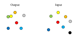
(a) Hard neighborhood matching

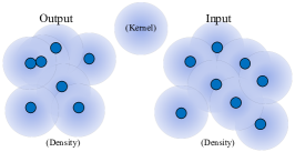
(b) Soft neighborhood matching

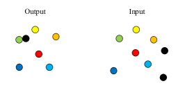
(c) Robust neighborhood matching

Figure 6. Different neighborhood matching methods. In LABEL:sub@fig:hard_neighborhood_matching each sample in the output (left) is forced to match with another one in the input (right), which could be problematic since some output samples are outliers and should not be matched to any input samples, and some output samples might be missing in the current iteration of optimization. Matched samples are with the same color. Black indicates unmatched. In LABEL:sub@fig:soft_neighborhood_matching samples are not explicitly matched but the neighborhood is matched as a whole, by transforming the samples with density kernels [Roveri et al., 2015]. There is no one-to-one correspondence between samples, and thus it is not easy to integrate with various sample attributes. Instead, we propose robust neighborhood matching LABEL:sub@fig:robust_neighborhood_matching to generate high-quality sample distributions to accommodate various types of patterns. We allow output samples to be unmatched if it can result in high matching cost increase. In the above example, the yellow output sample in LABEL:sub@fig:hard_neighborhood_matching destroys the hard neighborhood matching and forces other (orange, and gray) samples to be less matched, while our robust matching leaves the bad sample unmatched.

Instead, we propose to use a robust neighborhood matching that explicitly considers outliers in the output to address these issues (Figure 6c). An output sample is either matched with an input sample or unmatched as an outlier with additional cost $c$. We apply the Hungarian algorithm to compute the matchings between input $\mathbf{n}(s_{i})$ and output neighborhoods $\mathbf{n}(s_{o})$. The input of the Hungarian algorithm is a cost matrix where each entry indicates the matching cost between an output and an input sample. Inspired by [Riesen and Bunke, 2009], we define our cost matrix $\mathcal{C}\in\mathbb{R}^{N_{\mathbf{n}o}\times(N_{\mathbf{n}i}+N_{\mathbf{n}o})}$ as:

(10) $$\mathcal{C} =\left[\begin{array}[]{c|c}\mathcal{C}_{m}&\mathcal{C}_{u}\end{array}\right]$$

(11) $$\mathcal{C}_{m} =\left[\begin{matrix}\hat{\mathbf{u}}_{s_{o}s_{i}}(s_{o}^{\prime 1},s_{i}^{\prime 1})&\hat{\mathbf{u}}_{s_{o}s_{i}}(s_{o}^{\prime 1},s_{i}^{\prime 2})&\cdots&\hat{\mathbf{u}}_{s_{o}s_{i}}(s_{o}^{\prime 1},s_{i}^{\prime N_{\mathbf{n}i}})\\ \hat{\mathbf{u}}_{s_{o}s_{i}}(s_{o}^{\prime 2},s_{i}^{\prime 1})&\hat{\mathbf{u}}_{s_{o}s_{i}}(s_{o}^{\prime 2},s_{i}^{\prime 2})&\cdots&\hat{\mathbf{u}}_{s_{o}s_{i}}(s_{o}^{\prime 2},s_{i}^{\prime N_{\mathbf{n}i}})\\ \vdots&\vdots&\ddots&\vdots\\ \hat{\mathbf{u}}_{s_{o}s_{i}}(s_{o}^{\prime N_{\mathbf{n}o}},s_{i}^{\prime 1})&\hat{\mathbf{u}}_{s_{o}s_{i}}(s_{o}^{\prime N_{\mathbf{n}o}},s_{i}^{\prime 2})&\cdots&\hat{\mathbf{u}}_{s_{o}s_{i}}(s_{o}^{\prime N_{\mathbf{n}o}},s_{i}^{\prime N_{\mathbf{n}i}})\\ \end{matrix}\right]$$

(12) $$\mathcal{C}_{u} =\left[\begin{matrix}c_{1}&c_{1}&\cdots&c_{1}\\ c_{2}&c_{2}&\cdots&c_{2}\\ \vdots&\vdots&\vdots&\vdots\\ c_{N_{\mathbf{n}o}}&c_{N_{\mathbf{n}o}}&\cdots&c_{N_{\mathbf{n}o}}\end{matrix}\right],$$

where the superscripts of $s_{o}^{\prime}$ or $s_{i}^{\prime}$ represent the index of a sample within $\mathbf{n}(s_{o})$ or $\mathbf{n}(s_{i})$. There are $N_{\mathbf{n}i}$ and $N_{\mathbf{n}o}$ samples within $\mathbf{n}(s_{i})$ and $\mathbf{n}(s_{o})$, respectively. In [Ma et al., 2013], the sample matching is computed via only the $\mathcal{C}_{m}$ part of $\mathcal{C}$, in which case every output sample should be matched. Our cost matrix is augmented with the $\mathcal{C}_{u}$ side, where each entry represents the cost of unmatched outliers in $\mathbf{n}(s_{o})$. We make sure there are enough samples in the input neighborhood so that an output sample would not be matched only when it is an outlier that would result in a high cost increase in matching. For the same reason, we do not take missing output samples into account in the cost matrix formulation.

In our implementation, $c_{k}$ is set as $\min(2,1.2+0.4|\boldsymbol{\mathcal{E}}(s_{o}^{k})|)\delta$ if the output sample $s_{o}^{k}$ is from a continuous pattern, and $1.5\times$ average nearest neighbor distance if $s_{o}^{k}$ is from a discrete element. In an interactive system, we may synthesize predictions near the provided exemplars. If $s_{o}^{k}$ is from the exemplars, $c_{k}=\infty$ because none of the samples from the exemplars are outliers and all of them should be matched.

In a neighborhood, there might be samples from both discrete elements and continuous structures. We only match samples from the same type of patterns and with the same id, i.e. continuous structures only match with continuous structures (negative id), and discrete elements only match the same discrete elements and their samples with the same (non-negative) ids.

4.3. Pattern Synthesis

Based on our pattern representation (Section 4.1) and similarity measures (Section 4.2), we now describe how to synthesize an output similar to a given input.

4.3.1. Optimization Objective

We synthesize output predictions $\mathcal{O}$ via optimizing the following objective:

(13) $$E(\mathcal{O})=\sum_{\begin{subarray}{c}s_{i}=m(s_{o}),s_{o}\in\mathcal{O}\end{subarray}}\left\|\mathbf{n}(s_{o})-\mathbf{n}(s_{i})\right\|+\Theta(\mathcal{O},\mathcal{D}).$$

where $s_{o}$ is matched with $s_{i}$. This energy sums up the similarity between every $\mathbf{n}(s_{o})$ in $\mathcal{O}$ and its most similar $\mathbf{n}(s_{i})$ via Equation 7. $\Theta(\mathcal{O},\mathcal{D})$ is the domain constraint term [Dumas et al., 2018] to encourage the synthesized samples to stay within the user-specified domain $\mathcal{D}$.

The pattern optimization framework adopts an EM-like strategy to minimize Equation 13, by iterating the search and assignment steps as detailed below.

4.3.2. Initialization

Similar to prior patch-based texture synthesis methods [Efros and Freeman, 2001; Liang et al., 2001], we copy new patches one-by-one with similar boundary patterns to existing patches for initialization. Each next patch is selected to ensure high similarity (as evaluated by Equation 7) in the overlapped boundary regions with existing patches. In the overlapping regions, we only copy samples unmatched with any sample in the existing patches. We make sure that the initialized samples are within the output domain $\mathcal{D}$ by removing samples outside it. We copy discrete elements in wholes like [Ma et al., 2011]. In Section 5, we will show the robustness of our method to random sample initializations (Figure 14). But patch-based initialization makes the algorithm converge faster, contributing to the responsiveness of the interface. For simplicity, we do not copy edges in the initialization step.

(a) Matched neighborhood pair 1

(b) Matched neighborhood pair 2

(c) Matched neighborhood pair 3

(d) Assign existence

Figure 7. Existence assignment example. We visualize how to compute confidences of existence of output samples $i(s_{o})$ (Equations 16 and 1) from a set of matched input and output neighborhoods. LABEL:sub@fig:existence_assign:n1 LABEL:sub@fig:existence_assign:n2 LABEL:sub@fig:existence_assign:n3 show three pairs of matched input and output neighborhoods centered at different samples (shown in red) over the same set of samples. Matched samples are in the same color. Empty black circles indicate samples outside a neighborhood. Solid black circles indicate samples within a neighborhood but unmatched. The black cross sample in LABEL:sub@fig:existence_assign:merged has $i(s_{o})=0$, since it is unmatched with any $s_{i}$ ($i(s_{i})=0$) in LABEL:sub@fig:existence_assign:n1 and LABEL:sub@fig:existence_assign:n2. The green sample in LABEL:sub@fig:existence_assign:merged has confidence $i(s_{o})=\frac{2}{3}$: in the three pairs of neighborhoods, there are two pairs LABEL:sub@fig:existence_assign:n1 and LABEL:sub@fig:existence_assign:n3 where each has an unmatched input sample, which indicates there could be a missing sample in the output located at approximately the same location relative to its neighborhood center; the two unmatched input samples are merged to generate the green output sample in LABEL:sub@fig:existence_assign:merged.

(a) Initialization

(b) Step 1

(c) Step 2

(d) Step 3

(e) Step 4

Figure 8. Edge assignment example. This example illustrates how to solve Equation 17 for edge assignment by solving Equation 22 in a loop. Each step LABEL:sub@fig:existence_assign:1-LABEL:sub@fig:existence_assign:4 solves Equation 22 once. There are four samples and four potential edges (with $\overline{i}(e)>0$). The numbers near edges or samples indicate the expected confidence of existence $\overline{i}(e)$ of the edges or the expected number of edges $|\overline{\boldsymbol{\mathcal{E}}}(s)|$ associated with samples (e.g. $\overline{i}(e_{2})=0.8$, $|\overline{\boldsymbol{\mathcal{E}}}(s_{2})|=1.9$). In LABEL:sub@fig:existence_assign:init, we initialize all $i(e)=0$ and sort all potential edges by its $\overline{i}$ from the largest to the smallest: $e_{1}$ is the one with the largest $\overline{i}$ and $e_{4}$ is the one with the smallest. The optimization loops from $e_{1}$ LABEL:sub@fig:existence_assign:1 to $e_{4}$ LABEL:sub@fig:existence_assign:4 in decreasing $\overline{i}(e)$ values. The number below each $E_{e}^{\prime}\left(i(e)\right)$ is its computed value (e.g. $E_{e}^{\prime}\left(i(e_{1})=1\right)=|i(e_{1})-\overline{i}(e_{1})|+|\boldsymbol{\mathcal{E}}(s_{1})-\overline{\boldsymbol{\mathcal{E}}}(s_{1})|+|\boldsymbol{\mathcal{E}}(s_{2})-\overline{\boldsymbol{\mathcal{E}}}(s_{2})|=|1-1|+|1-1|+|1-1.9|=0.9$). The light green edges are not optimized with initial values $i(e)=0$. The dark green edges are optimized with $i(e)=1$. The red edge is optimized with $i(e)=0$. The light red indicates there is no edge after optimization.

4.3.3. Search Step

We adopt PatchMatch [Barnes et al., 2009; Chen et al., 2012] to compute approximate nearest neighbors (ANN) for each output sample. The standard PatchMatch algorithm 1) randomly generates the initial nearest neighbor field, and 2) alternates between propagation and search steps by traversing the regular image grid in a scanline order. Initially, we generate the ANN by randomly assigning an output sample to an input sample (with identical sample id for discrete elements). One issue is how to choose a sample traversal order. We follow the steps from [Chen et al., 2012] which works on meshes. We build a simple graph by connecting each sample with its $k$-nearest neighbors ($k=8$ in our implemenetation), and perform breadth-first search. In the next iteration, the traversal starts from the last sample in the most recent sequence.

In our implementation, for the random search step, the maximum window size is 150, and the minimum size is 25, and the search window is exponentially decreased with factor 2. In each pattern optimization step, we need to compute an ANN. In two consecutive steps, the output sample distributions are similar. So the previous ANN is used to initialize the subsequent patch match algorithm. Since the initialization is close to the converged ANN, a small number (2) of Patch Match iterations is used, except for the initial step at each level of hierarchical synthesis (Section 4.3.5), which uses 5 iterations. Our patch match implementation is parallelized by equally dividing the output domain into regions, the number of which equals to that of threads. The search step consumes most of the computation time needed by the synthesis. The computational complexity of the search step in an optimization step is $O(n_{\mathcal{O}}N_{\mathbf{n}}^{3})$, where $n_{\mathcal{O}}$ is the total number of output samples and $N_{\mathbf{n}}$ is the average number of samples within neighborhoods. Please refer to Appendix C for more details.

4.3.4. Assignment Step

Here, we describe how to determine the values of sample positions $\mathbf{p}$, attributes including edge $\boldsymbol{\mathcal{E}}$ and orientation $\mathbf{o}$, as well as sample existence $i$. The assignments of these different quantities are extended from the assignment step of pixel colors [Kwatra et al., 2005] and sample positions [Ma et al., 2011] by taking votes from overlapping output neighborhoods at the same entity (such as sample or edge). In particular, discrete samples only have sample id attributes $q$, which is used in the search step to make sure only samples with the same $q$ are matched. Thus, only position assignment is deployed for discrete samples.

Position assignment

For each output sample $s_{o}$ and its neighbor $s_{o}^{\prime}$, there is a set of matched input sample pairs $\left(s_{i},s_{i}^{\prime}\right)$ provided by the previous search step. The estimated distance $\hat{\mathbf{p}}(s_{o},s_{o}^{\prime})$ between $s_{o}$ and $s_{o}^{\prime}$ is

(14) $$\hat{\mathbf{p}}(s_{o},s_{o}^{\prime})\approx\mathbf{p}(s_{i})-\mathbf{p}(s_{i}^{\prime}).$$

We use least squares [Ma et al., 2011] to estimate $\mathbf{p}(s_{o})$ by

(15) $$\operatorname*{arg\,min}_{\{\mathbf{p}(s_{o})\}}\sum_{s_{o}\in\mathcal{O}}\sum_{s_{o}^{\prime}\in\mathbf{n}(s_{o})}\left\|\hat{\mathbf{p}}(s_{o},s_{o}^{\prime})-\left(\mathbf{p}(s_{i})-\mathbf{p}(s_{i}^{\prime})\right)\right\|^{2}+\sum_{s_{o}\notin\mathcal{D}}\|\hat{\mathbf{p}}(s_{o},\mathcal{D})\|^{2}.$$

The second term in Equation 15 is the domain constraint to encourage output samples to stay within $\mathcal{D}$, where $\hat{\mathbf{p}}(s_{o},\mathcal{D})$ is the shortest vector from $s_{o}$ to the boundary of $\mathcal{D}$, and $s_{o}\notin\mathcal{D}$ indicates $s_{o}$ is outside $\mathcal{D}$.

Existence assignment

Our method adjusts the number of samples within local regions during the synthesis process for better quality. The number of samples is optimized via existence $i$ assignment, again via a voting scheme:

(16) $$\operatorname*{arg\,min}_{i(s_{o})\in[0\ 1]}\sum_{s_{i}\in\{s_{i}\}}\left|i(s_{o})-i(s_{i})\right|^{2},$$

where $s_{i}$ runs through the set $\{s_{i}\}$ we collect during neighborhood matching, i.e. the corresponding input samples of an output sample from overlapping input neighborhoods. $i(s_{i})=0$ if $s_{o}$ is not matched with any $s_{i}$ in a pair of matched input and output neighborhoods, and $i(s_{i})=1$ otherwise. Equation 16 computes the confidence of existence $i(s_{o})\in[0\ 1]$ of an output sample $s_{o}$. Every iteration , we remove output samples $s_{o}$ whose $i(s_{o})<0.5$. The above assignment step is applied to samples that are already in the output sample distribution. To add back missing output samples, we first generate candidate samples, merge them as output samples, and pick those with $i(s_{o})>0.5$ as added output samples. The energy in Equation 16 is not guaranteed to decrease immediately after sample addition or removal, but it will generally decrease through iterations. Please refer to Figure 7 for an example and Appendix A for more algorithm details.

Edge assignment

We assign edges by optimizing the following objective:

(17) $$\operatorname*{arg\,min}_{\{i(e_{s_{o}s_{o}^{\prime}})\in\{0,1\}\}}\sum_{\{e_{s_{o}s_{o}^{\prime}}\}}\left|i(e_{s_{o}s_{o}^{\prime}})-\overline{i}(e_{s_{o}s_{o}^{\prime}})\right|+\sum_{\{s_{o}\}}\left||\boldsymbol{\mathcal{E}}(s_{o})|-|\overline{\boldsymbol{\mathcal{E}}}(s_{o})|\right|,$$

where the first term computes the difference between the actual and expected edge confidences $\overline{i}(e_{s_{o}s_{o}^{\prime}})\in[0\ 1]$. $\overline{i}$ is the vote by overlapping input neighborhoods on the same edge, computed using least squares by replacing samples in Equation 16 with edges. $\{e_{s_{o}s_{o}^{\prime}}\}$ is the set of edges that have $\overline{i}(e_{s_{o}s_{o}^{\prime}})>0$, and there is no edge between $s_{o}$ and $s_{o}^{\prime}$ if $\overline{i}(e_{s_{o}s_{o}^{\prime}})=0$. The second term computes the differences between the optimized number of edges $|\boldsymbol{\mathcal{E}}(s_{o})|$ and the expected number of edges $|\overline{\boldsymbol{\mathcal{E}}}(s_{o})|$ connected to $s_{o}$. $|\overline{\boldsymbol{\mathcal{E}}}(s_{o})|$ is similarly computed by voting from overlapping output neighborhoods on the same sample $s_{o}$:

(18) $$\operatorname*{arg\,min}_{|\overline{\boldsymbol{\mathcal{E}}}(s_{o})|}\sum_{s_{i}\in\{s_{i}\}}\left||\overline{\boldsymbol{\mathcal{E}}}(s_{o})|-|\boldsymbol{\mathcal{E}}(s_{i})|\right|^{2}.$$

Basically, we compute the average of $\{|\boldsymbol{\mathcal{E}}(s_{i})|\}$. In sum, the first term is edge-centric while the second is sample-centric.

It is non-trivial to optimize Equation 17, where the optimization variables $\{i(e_{s_{o}s_{o}^{\prime}})\}$ are binary. Thus, we solve it in a greedy fashion. We initialize all $i(e_{s_{o}s_{o}^{\prime}})=0$. We sort output edges $\{e_{s_{o}s_{o}^{\prime}}\}$ by its expected confidence of existence $\overline{i}(e_{s_{o}s_{o}^{\prime}})$, and optimize $i(e_{s_{o}s_{o}^{\prime}})$ greedily by looping over the sorted $\{e_{s_{o}s_{o}^{\prime}}\}$ in decreasing confidence. For each $e_{s_{o}s_{o}^{\prime}}$, we decide whether $i(e_{s_{o}s_{o}^{\prime}})=$ $0$ or $1$ by choosing the one that minimizes Equation 17. In other words, the multivariate optimization problem (Equation 17) is optimized by solving univariate optimization problems in a loop. By decomposing the optimization variables in Equation 17 from a set of edges $\{i(e_{s_{o}s_{o}^{\prime}})\}$ to a single edge $i(e_{s_{o}^{*}s_{o}^{*\prime}})$ to be optimized and the rest, the univariate version of Equation 17 can be written as:

(19) $$\operatorname*{arg\,min}_{i(e_{s_{o}^{*}s_{o}^{*\prime}})\in\{0,1\}}E_{e}^{\prime}+E_{e}^{\prime\prime},$$

where

(20) $$\begin{split}E_{e}^{\prime}\left(i(e_{s_{o}^{*}s_{o}^{*\prime}})\right)&=\left|i(e_{s_{o}^{*}s_{o}^{*\prime}})-\overline{i}(e_{s_{o}^{*}s_{o}^{*\prime}})\right|+\\ &\left||\boldsymbol{\mathcal{E}}(s_{o}^{*})|-|\overline{\boldsymbol{\mathcal{E}}}(s_{o}^{*})|\right|+\left||\boldsymbol{\mathcal{E}}(s_{o}^{*\prime})|-|\overline{\boldsymbol{\mathcal{E}}}(s_{o}^{*\prime})|\right|,\end{split}$$

(21) $$\begin{split}E_{e}^{\prime\prime}\left(i(e_{s_{o}^{*}s_{o}^{*\prime}})\right)&=\sum_{\{e_{s_{o}s_{o}^{\prime}}\}\ominus e_{s_{o}^{*}s_{o}^{*\prime}}}\left|i(e_{s_{o}s_{o}^{\prime}})-\overline{i}(e_{s_{o}s_{o}^{\prime}})\right|+\\ &\sum_{\{s_{o}\}\ominus\{s_{o}^{*},s_{o}^{*\prime}\}}\left||\boldsymbol{\mathcal{E}}(s_{o})|-|\overline{\boldsymbol{\mathcal{E}}}(s_{o})|\right|.\end{split}$$

Since $E_{e}^{\prime\prime}$ is a constant in Equation 19, it is equivalent to:

(22) $$\operatorname*{arg\,min}_{i(e_{s_{o}^{*}s_{o}^{*\prime}})\in\{0,1\}}E_{e}^{\prime}.$$

Equation 22 can be solved with brute-force search. The search space is 2 ($\{0,1\}$). Figure 8 illustrates how to solve Equation 17 by solving Equation 22 in a loop.

Orientation assignment

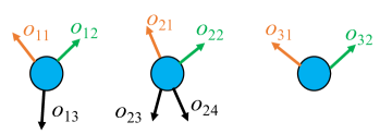
(a) $\{\mathbf{o}(s_{i})\}$

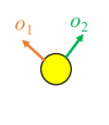
(b) $\mathbf{o}(s_{o})$

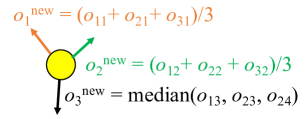
(c) Updated LABEL:sub@fig:orientation_assign:output

Figure 9. Orientation assignment example. This example illustrates the orientation assignment step when $N_{\mathbf{o}}(s_{o})$ is increased from $2$ to $3$. The output sample LABEL:sub@fig:orientation_assign:output is matched with the three input samples LABEL:sub@fig:orientation_assign:input. Matched orientations $o$ (arrows) are visualized in the same colors. Unmatched inputs $o$ are in black. LABEL:sub@fig:orientation_assign:assign shows the updated orientations of the output sample. The orange $o_{1}^{\text{new}}$ and green orientations $o_{2}^{\text{new}}$ are updated by averaging matched input orientations. The black output orientation $o_{3}^{\text{new}}$ is newly added by choosing the median from three unmatched orientations ($o_{13}$,$o_{23}$,$o_{24}$) in LABEL:sub@fig:orientation_assign:input.

In the search step (Section 4.3.3), each $\mathbf{o}(s_{o})$ is matched with a set of $\{\mathbf{o}(s_{i})\}$ associated with input samples coming from different input neighborhoods, and each entry $o(s_{o})\in\mathbf{o}(s_{o})$ has been matched with a $o(s_{i})\in\mathbf{o}(s_{i})$. The local orientation attribute $\mathbf{o}(s_{o})$ is updated by a voting scheme among $\{\mathbf{o}(s_{i})\}$, where $\{\mathbf{o}(s_{i})\}$ could have different lengths across different $s_{i}$.

We optimize both dimension $N_{\mathbf{o}}$ and value of entries $o$ in order. In the input exemplar, the number of orientation entries $N_{\mathbf{o}}(s_{i})$ equals $|\boldsymbol{\mathcal{E}}(s_{i})|$. Thus $N_{\mathbf{o}}$ can be computed like in Equation 18 and rounding the result as integers. Essentially, we are trying to find an integer $N_{\mathbf{o}}(s_{o})$ that is the closest to the arithmetic average of $\{N_{\mathbf{o}}(s_{i})\}$.

Similarly, we can update the values $o(s_{o})$ in $\mathbf{o}(s_{o})$ using the same voting scheme to Equations 16 and 18. A special case is when $N_{\mathbf{o}}(s_{o})$ is updated to a new value (changing $\mathbf{o}(s_{o})$ vector length). In this case, we will need to add or remove one or several entries to or from the original $\mathbf{o}(s_{o})$. To remove an entry from $\mathbf{o}(s_{o})$, we pick the one whose matched set of input votes $\{o(s_{i})\}$ has the largest variance. (We have experimented with another strategy that removes $o(s_{o})$ whose matched set of input votes $\{o(s_{i})\}$ has the least number of entries, but have not found visible differences to the maximum variance strategy above.) To add an entry to $\mathbf{o}(s_{o})$, we collect orientation entries $\{o^{\prime}(s_{i})\}$ from the input samples that remain unmatched to any orientation entries $\mathbf{o}(s_{o})$ of the matched output sample, and add a new entry $o(s_{o})$ into $\mathbf{o}(s_{o})$ as the median from the unmatched set $\{o^{\prime}(s_{i})\}$. An example is illustrated in Figure 9. In the rare case where we need to add more than one entry to $\mathbf{o}(s_{o})$, we randomly choose from $\{o^{\prime}(s_{i})\}$ after the median is used for the first add-on.

4.3.5. Hierarchical Synthesis

(a) Leaves

(b)

(c)

(d)

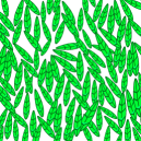
(e)

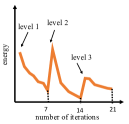
(f)

(g) Exemplar

(h) Initial step

(i) First level

(j) Second level

(k) Third level

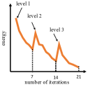
(l) Energy plot

Figure 10. Hierarchical synthesis visualization. The hierarchical synthesis proceeds from the coarsest (first level) to the finest levels (third level), with upsampling sample representations (Figure 5b). The hierarchical synthesis gradually refines the pattern from large to small scale structures. Note that the initialization has fewer elements than required (top row), hence our existence optimization adaptively controls the total number of elements.

Instead of using a single-resolution representation [Ma et al., 2011], we apply a hierarchical representation (Section 4.1.1) for multi-resolution synthesis. We first synthesize the predictions at a coarse level using sparse representation, and then reconstruct the patterns based on sparse samples. We continue this process with a denser and denser pattern representation. Figure 5b shows an example of multi-resolution element representation. For continuous structures, the sampling distance $\delta$ of continuous pattern is gradually increasing with respect to the level of hierarchy. During synthesis, we use multi-scale neighborhood sizes to keep both large and local structures. The neighborhood size is gradually reduced at different hierarchies. In our implementation, at each hierarchy, there are 7 search-assignment iterations. See Figure 10 for an example.

4.4. Pattern Reconstruction

The reconstruction step takes a synthesized pattern representation as input to generate output patterns that may consist of discrete elements and continuous structures.

4.4.1. Discrete Elements

For discrete elements, each sample is uniquely associated with an element. The reconstruction is to transform the element shapes by treating samples as control points. Specifically, we assume similarity transform to reconstruct the elements.

4.4.2. Continuous Structures

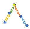
(a) 2-neighbor $s$

(b) 2 paths from LABEL:sub@fig:curve_recon:graph:1

(c) 1 path from LABEL:sub@fig:curve_recon:graph:1

(d) $>$2 neighbor $s$

(e) Recon from LABEL:sub@fig:curve_recon:graph

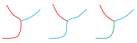
(f) Other possible reconstructions from LABEL:sub@fig:curve_recon:graph

Figure 11. Curve reconstruction from a graph using orientation attributes. If we only consider the different statuses of the yellow sample in LABEL:sub@fig:curve_recon:graph:1, there are two possible reconstructions LABEL:sub@fig:curve_recon:good_recon:1LABEL:sub@fig:curve_recon:bad_recon:1, depending on whether it is a junction LABEL:sub@fig:curve_recon:good_recon:1 or path LABEL:sub@fig:curve_recon:bad_recon:1 sample. If we only consider the different statuses of the red sample in LABEL:sub@fig:curve_recon:graph, there are four possible reconstructions LABEL:sub@fig:curve_recon:good_reconLABEL:sub@fig:curve_recon:bad_recon, depending on the red sample is included within which two or three paths. For the yellow (in LABEL:sub@fig:curve_recon:graph:1) and red samples (in LABEL:sub@fig:curve_recon:graph), we decide the reconstruction by examining its associated local orientation attribute and the fact a pair of local orientations of a sample should be opposite if the sample is included within the path. Our algorithm will reconstruct LABEL:sub@fig:curve_recon:good_recon:1 from LABEL:sub@fig:curve_recon:graph:1 and LABEL:sub@fig:curve_recon:good_recon from LABEL:sub@fig:curve_recon:graph.

We have synthesized a graph whose sample positions and edge connections represent the topology of the output (Section 4.3). However, these edges are piecewise linear, and they thus capture only connectivity/topology, but not shape/geometry information. The original continuous patterns can be composed of smooth paths (e.g. quadratic Bézier curves). Therefore, we need to reconstruct paths from the graph samples and edges. The samples are used as control points of Bézier curves.

Next, we talk about how to identify which sample and which edge are included within which path. This process relies on the synthesized sample orientation attributes $\mathbf{o}$.

Samples with only one neighbor are unambiguous and thus only included within one path. Samples with only two neighbors could be included in one path (all blue samples with two neighbors in Figure 11) as path samples, or two paths as junction samples (e.g. the yellow sample in Figure 11a). Samples with more than two neighbors are junction samples (e.g. the red sample in Figure 11d) that are included in multiple potential paths.

To disambiguate these cases, we examine a sample’s local orientations $\mathbf{o}(s)$. Since $o\in\mathbf{o}(s)$ should be tangent to the sample’s local path, if a sample $s$ has a pair of orientations $o(s)$ that are almost opposite ($8\pi/9<$ absolute orientation difference $<10\pi/9$), it will suggest that the sample is included inside a path as opposed to at the ends of a path. Therefore, there are three steps to reconstruct a pattern without ambiguity. First, we identify pairs of local path orientations $o(s)$ (if any) that are opposite (e.g., a pair of arrows associated with 2-neighbor blue samples in Figures 11a and 11d, or the orange and green ones associated with the red junction sample in Figure 11d). Second, we match local orientations $o(s)$ with edges $e\in\boldsymbol{\mathcal{E}}(s)$ connected to the sample using the Hungarian algorithm by minimizing the sum of absolute difference between local orientation and edge angles. The arrows and graph edges in Figures 11a and 11d with the same colors are matched. Third, we generate a path by including edges that are connected together and matched with opposite orientations. A Bézier curve is generated by interpolating samples along a path. This reconstruction strategy using $\mathbf{o}$ can help preserving the original curve shapes, as demonstrated in Figure 15.

5. Evaluation

We evaluate our method with sample results, ablation studies, and comparisons with existing art. We will make our code repository [Tu, 2020] public to facilitate future research.

5.1. Results

(a) Zentangle

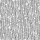
(b)

(c) Diffusion

(d)

(e) Wet flow

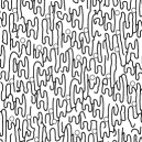
(f)

(g) Brick wall

(h)

(i) Fence

(j)

(k) Blocks

(l)

(m) Heart

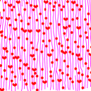
(n)

(o) Curve grid

(p)

(q) Isocontour

(r)

(s) Circuit

(t)

(u) Chain

(v)

(w) Fabric

(x)

Figure 12. Automatic synthesis results by our method. Within each pair of images, the input exemplar is smaller and shown on the left, the automatic synthesis result is bigger and shown on the right.

(a) Uneven bricks

(b) Auto

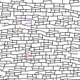
(c) User 16 + 11

(d) Edited

(e) Zigzag

(f) Auto

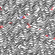
(g) User 11 + 2

(h) Edited

(i) Prisma

(j) Auto

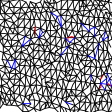
(k) User 5 + 28

(l) Edited

(m) Waves (small)

(n) Auto

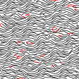
(o) User 21 + 0

(p) Edited

Figure 13. Automatic synthesis and user-assisted results. We count the number of user operations needed for correcting artifacts. Red indicates the number of rejection and blue the number of manual path drawing.

Our method can automatically synthesize satisfactory results for a variety of patterns without user intervention, as exemplified in Figures 1, 12 and 13 and our (full) results in Figures 10, 14, 16, 15 and 2. However, like existing techniques, our method might not always produce what users would like to have, and some artifacts can be visible in local regions (such as unfinished or dangling components in Figure 1a and Figure 2g or inconsistent curvatures in Figure 10k bottom) and global structures (such as the regular and warped grids in Figures 12h and 12p, the rectangular blocks in Figure 12l, and the straight lines in Figures 1e and 12t). For further quality improvement and customization, users can also interactively edit the system suggestions via our system interface, as demonstrated in Figure 13. Unless otherwise noted, all our results are produced with three hierarchies using neigborhood radii $r\in\{60,50,40\}$ with sampling distance $\delta\in\{40,30,25\}$, while the longer side of bounding box of exemplars are varying between 250 and 500. Our method is robust to variations of neighborhood radii. See Appendix B for more details about our parameter settings.

5.2. Ablation Study

(a) Voronoi

(b)

(c)

(d)

(e)

(f) Tree

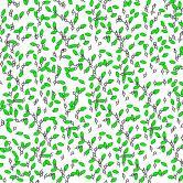
(g) Patch-based initialization

(h) Patch-based final output

(i) Random sample initialization

(j) Random sample final output

Figure 14. Algorithm robustness to different initialization. Our algorithm can generate similar results with both patch-based or random initialization.

Although we use patch-based methods for initialization in our implementation, our algorithm is robust to different initial conditions (Figure 14), even if the initial sample distribution is randomly distributed (white noise). Figure 15 is the ablation study for the orientation attribute $\mathbf{o}$. Figure 16 shows other components of our algorithm. Without the edge term (Equation 5) or robust matching (Section 4.2.3) in the search step, our algorithm produces lower quality results with obvious artifacts. Without existence assignment (the third paragraph in Section 4.3.4), the algorithm cannot automatically adjust the number of samples within local regions and can produce empty space or extra broken curves.

(a) Crocodile skin

(b) With $\mathbf{o}$

(c) Zoom-in of LABEL:sub@fig:curve_recon:ours:1

(d) Without $\mathbf{o}$

(e) Flame

(f) With $\mathbf{o}$

(g) Zoom-in of LABEL:sub@fig:curve_recon:ours:2

(h) Without $\mathbf{o}$

Figure 15. Ablation study for $\mathbf{o}$. The orientation attribute $\mathbf{o}$ is useful to faithfully recover curve appearance in the exemplars. In the ”crocodile skin” example, the curves should be smooth at junction; in the ”flame” example, the curves should be sharp at the flame tip.

(a) Fish scale

(b)

(c)

(d)

(e)

(f) Roof tiles

(g) Without edge search

(h) Without robust matching

(i) Without existence assignment

(j) Full result

Figure 16. Ablation study. Without using edges (Equation 5) in the search step (the second column) or robust matching (Section 4.2.3) that considers outliers (the third column), the algorithm produces lower quality results. Without existence assignment (the third paragraph in Section 4.3.4), the algorithm produces broken curves and empty space due to outliers and missing samples (the forth column). Our results are shown in the last column.

5.3. Comparison to Previous Methods

To our knowledge, there is no previous example-based method that can generate the types of patterns we target. The sample-based methods in [Ma et al., 2011; Roveri et al., 2015; Tu et al., 2019] are the most related. We compare against [Ma et al., 2011; Roveri et al., 2015] and a state-of-art point distribution synthesis method in [Tu et al., 2019] which applies convolutional neural networks to preserve both local and global structures. As shown in Figure 2, our method can produce better spatial sample distributions than [Ma et al., 2011; Roveri et al., 2015; Tu et al., 2019]. Note that we compare only sample distributions in Figure 2 since it is unclear how to reconstruct continuous curve patterns from synthesized samples without connectivity [Ma et al., 2011; Roveri et al., 2015; Tu et al., 2019].

We also enhance [Ma et al., 2011] for comparisons, by incorporating it with the sample connectivity (Figure 5d) and edge assignment step (Equation 17), but without the edge set difference (Equation 5) and robust matching (Section 4.2.3) in the search step, as well as without the existence assignment step (the third paragraph in Section 4.3.4). As shown in Figure 17, our method can generate better results than the enhanced version of [Ma et al., 2011]. Unlike for [Ma et al., 2011], we are unable to enhance [Tu et al., 2019; Roveri et al., 2015] due to the lack of one-to-one sample correspondences which are needed for the edge assignment step.

(a) Waves (large)

(b)

(c)

(d) Roof tiles

(e)

(f)

(g) Fish scale

(h) Enhanced [Ma et al., 2011]

(i) Ours

(j) Wood ring

(k) Enhanced [Ma et al., 2011]

(l) Ours

Figure 17. Comparison of our algorithm with enhanced [Ma et al., 2011]. We compare our methods to an enhanced version of [Ma et al., 2011] that incorporates our ideas, including the sample connectivity and edge assignment.

6. Conclusions, Limitations, and Future Work

Repetitive patterns have many applications, whose creation has been a main focus of research in computer graphics and interactive techniques. This work focuses on methods and interfaces to help users author continuous curve patterns. Analysis and results of diverse patterns have demonstrated the promise of our approach.

(a) Input

(b) Output

(c) Input

(d) Ouptut

Figure 18. Failure case. Our algorithm fails to preserve the identifiable DNA-segment and tree-leaf elements within the continuous structures.

Like other neighborhood-based texture/pattern synthesis methods, our algorithm also assumes local properties and thus cannot capture global structures and may introduce stochastic variations, such as broken and distorted curves, as shown in Section 5.1. These artifacts can be reduced by other improvements, such as bidirectional similarity, additional feature masks, and smart initialization [Kaspar et al., 2015].

Our current reconstruction algorithm is based on Bézier curve interpolation, which might not preserve the exemplar curves. One possibility is to treat each curve segment like a discrete element and reconstruct via sample-based warping [Ma et al., 2011; Hsu et al., 2020], while ensuring that curve segments sharing common samples are well connected.

Our current algorithm treats discrete elements and continuous structures separately and thus might not preserve identifiable elements within continuous structures, as exemplified in Figure 18. A potential future work is to find a unified representation and approach for both discrete and continuous patterns.

The pattern synthesis requires nearest neighborhood searching for output samples, which can become computationally expensive for large outputs. This neighborhood searching process can be readily parallelized [Huang et al., 2007].

We focus on curves as the first step to handle continuous vector patterns. A next step is to incorporate more vector graphics features as parts of the sample/edge attributes, such as color and thickness, as well as higher dimensional primitives including 2D regions and 3D volumes [Takayama et al., 2010; Wang et al., 2010, 2011]. More controls can also be added to facilitate more diverse authoring effects such as local variations in scales and orientations [Hsu et al., 2020]. In addition to optimizing pattern appearance as in this work, adding mechanical structures constraints can facilitate the application of curve structures for rapid manufacturing [Zehnder et al., 2016; Chen et al., 2017, 2016; Zhou et al., 2014; Bian et al., 2018; Li et al., 2019].

Appendix A Existence Assignment

The algorithm for generating additional samples is shown in Algorithm 1.

1:  $\mathbf{function}$ GenerateNewOutputSamples($\{\mathbf{n}(s_{i}),\mathbf{n}(s_{o})\}$)

2:  $\{s_{o}^{c}\}\leftarrow\emptyset$ {candidate sample set}

3:  $\{\mathcal{S}\}\leftarrow\emptyset$ {$\mathcal{S}$ is a cluster that contains some candidate samples}

4:  $\{s_{o}\}\leftarrow\emptyset$ {new output sample set}

5:  for $\mathbf{n}(s_{i}),\mathbf{n}(s_{o})\in\{\mathbf{n}(s_{i}),\mathbf{n}(s_{o})\}$ do

6:     for $s_{i}^{\prime}\in\mathbf{n}(s_{i})$ do

7:        if $s_{i}^{\prime}$ is unmatched then

8:           Generate a candidate sample $s_{o}^{c}$ with $\mathbf{p}(s_{o}^{c})=\mathbf{p}(s_{i}^{\prime})-\mathbf{p}(s_{i})+\mathbf{p}(s_{o})$ and other attributes are the same to $s_{i}^{\prime}$

9:           $\{s_{o}^{c}\}\leftarrow\{s_{o}^{c}\}\cup s_{o}^{c}$

10:        end if

11:     end for

12:  end for

13:  for $s_{o}^{c}\in\{s_{o}^{c}\}$ do

14:     {Generate clusters from the candidate sample set by greedily looping over all candidates; more advanced clustering technique can be applied to replace this step}

15:     Find the $\mathcal{S}$ within $\{\mathcal{S}\}$ with nearest center to $s_{o}^{c}$

16:     if Distance($\mathcal{S},s_{o}^{c}$) ¡ $0.5\delta$  then

17:        {Distance($\mathcal{S},s_{o}^{c}$) computes the spatial distance between the center of $\mathcal{S}$ and $s_{o}^{c}$}

18:        $\mathcal{S}\leftarrow\mathcal{S}\cup s_{o}^{c}$

19:     else

20:        $\mathcal{S}^{\prime}\leftarrow\emptyset$

21:        $\mathcal{S}^{\prime}\leftarrow\mathcal{S}^{\prime}\cup s_{o}^{c}$

22:        $\{\mathcal{S}\}\leftarrow\{\mathcal{S}\}\cup\mathcal{S}^{\prime}$

23:     end if

24:  end for

25:  for $\mathcal{S}\in\{\mathcal{S}\}$ do

26:     create a new $s_{o}$ with averaged sample positions and attributes by merging all $\{s_{o}^{c}\}$ within $\mathcal{S}$

27:     $i(s_{o})\leftarrow\frac{\#\mathcal{S}}{\#\text{overlapping}\ \mathbf{n}\ \text{over}\ s_{o}}$ {existence assignment}

28:     if $i(s_{o})>0.5$ then

29:        $\{s_{o}\}\leftarrow s_{o}$

30:     end if

31:  end for

32:  return  $\{s_{o}\}$

Algorithm 1: Generating new output samples in existence assignment.

The candidate samples are generated from pairs of $\mathbf{n}(s_{i})$ and $\mathbf{n}(s_{o})$ (lines 5-12 in Algorithm 1). In a pair of $\mathbf{n}(s_{i})$ and $\mathbf{n}(s_{o})$, if there is an unmatched input sample $s_{i}^{\prime}$ in $\mathbf{n}(s_{i})$ (line 7), it will indicate the potential lack of an output sample, whose global position is $\mathbf{p}(s_{o}^{c})=\mathbf{p}(s_{i}^{\prime})-\mathbf{p}(s_{i})+\mathbf{p}(s_{o})$ located within $\mathbf{n}(s_{o})$, and attributes are the same to $s_{i}^{\prime}$ (line 8). The algorithm loops over all pairs of neighborhoods, each neighborhood pair may or may not produce new candidate samples. All these samples $s_{o}^{c}$ form a candidate sample set $\{s_{o}^{c}\}$. We group $\{s_{o}^{c}\}$ into clusters $\{\mathcal{S}\}$ (line 13-24) by assigning a sample to its nearest cluster $\mathcal{S}$ with distance between $s_{o}^{c}$ and the center of $\mathcal{S}$ smaller than $0.5\delta$ or otherwise create a new cluster $\mathcal{S}^{\prime}$ using the sample. For each cluster $\mathcal{S}\in\{\mathcal{S}\}$ (line 25-31), we merge all its candidate samples $\{s_{o}^{c}\}\in\mathcal{S}$ as one output sample $s_{o}$ by averaging their position and attributes using the same way as in the assignment step (Section 4.3.4). The existence of $s_{o}$ is assigned as the ratio of the number of candidates within $\mathcal{S}$ over the number of overlapping $\mathbf{n}$ over the position of $s_{o}$. For the sake of explanation, assume $i(s_{o})=1$, it means all $\mathbf{n}$ overlapping over $s_{o}$ produce one candidate sample on average, which suggests there could be missing samples, around $s_{o}$. Finally, $s_{o}$ with $i>0.5$ is added into the output sample distribution every iteration.

Appendix B Parameters

Table 2. Parameters. From left to right: neighborhood radii and sampling distances from lower to higher hierarchies. The parameters in the bottom part of the table share default values. Input size is bounding box size of input exemplar.

	$r$	$\delta$	input size
Figure 12h	$\{50,40,30\}$	$\{20,15,10\}$	350 $\times$ 200
Figure 12p	$\{60,50\}$	$\{40,30\}$	300 $\times$ 300
Figure 1e	$\{40,30,20\}$	$\{20,15,10\}$	250 $\times$ 250
Figure 13j	$\{60,50,40\}$	$\{40,30,30\}$	250 $\times$ 250
Figure 12f	$\{50,40,30\}$	$\{30,20,10\}$	300 $\times$ 350
Figure 1h	$\vdots$	$\vdots$	400 $\times$ 400
Figure 16e			400 $\times$ 300
Figure 12t			500 $\times$ 400
Figure 15b			350 $\times$ 300
Figure 12d	$\vdots$	$\vdots$	350 $\times$ 200
Figure 12x			300 $\times$ 300
Figure 12j			200 $\times$ 300
Figure 15f	$\{60,50,40\}$	$\{40,30,25\}$	300 $\times$ 300
Figure 12n			200 $\times$ 300
Figure 12r			400 $\times$ 400
Figure 14h			350 $\times$ 400
Figure 16j	$\vdots$	$\vdots$	400 $\times$ 250
Figure 1a			300 $\times$ 250
Figure 1d			350 $\times$ 300
Figure 14c			350 $\times$ 250
Figure 17c			500 $\times$ 300
Figure 13n	$\vdots$	$\vdots$	400 $\times$ 200
Figure 17l			250 $\times$ 350
Figure 12v			250 $\times$ 400
Figure 12b			300 $\times$ 300
Figure 13f			300 $\times$ 250

Table 2 lists the parameters for the results shown in the paper.

Appendix C Performance

Our current implementation in C++ is unoptimized. It takes about 160 seconds to synthesize a pattern with about 750, 1000, 1300 output samples and 30, 30, 20 samples on average within neighborhoods at each hierarchy, on a desktop with AMD Ryzen 9 3950 X 3.49 GHz 16-core processor and 32 GB RAM. The major computational burden is on the neighborhood searching process (Section 4.3.3). The computational complexity of neighborhood searching mainly depends on the number of samples and neighborhood radius. To compute the similarity and sample matching between a pair of neighborhoods, the Hungarian algorithm [Kuhn, 1955] has complexity $O(N_{\mathbf{n}}^{3})$ where $N_{\mathbf{n}}$ is the number of samples within a neighborhoood (assume all input and output neighborhoods have same number of samples). The patch match algorithm [Barnes et al., 2009] is composed of two alternating steps: propagation and random search. In an optimization step, there are the $an_{\mathcal{O}}I_{max}$ neighborhood matching computation where $a$ is a constant (in our implementation $a\approx 10$) which is related to the number of neighboring samples to a sample used in the propagation step and the range of random search, $n_{\mathcal{O}}$ is the total number of output samples, and $I_{max}$ is the maximum number of patch match iteration. The complexity of an optimization step is thus $O(n_{\mathcal{O}}N_{\mathbf{n}}^{3})$. Our algorithm has no more than 3 hierarchies and each hierarchy need about 7 steps. The lower hierarchy has less samples but a larger neighborhood radius (Section 4.3.5).

Appendix D Texture Synthesis

(a)

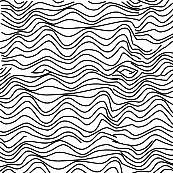
(b)

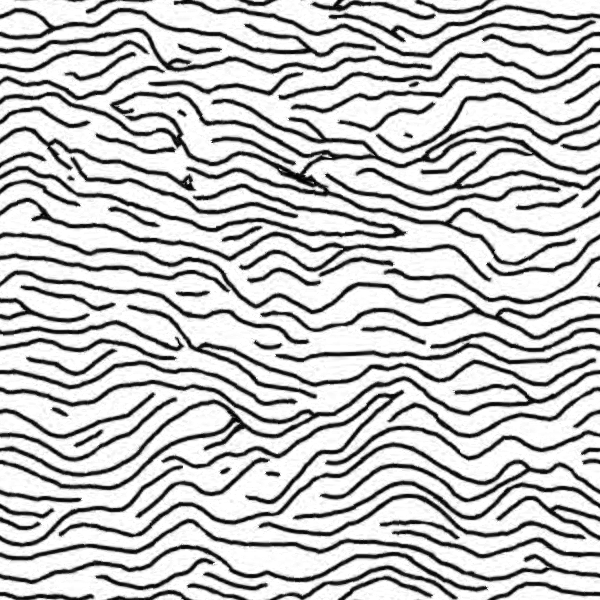
(c)

(d)

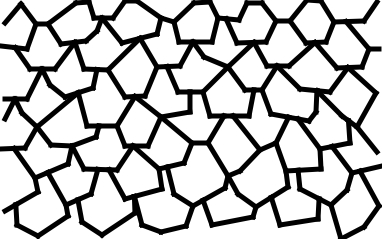
(e)

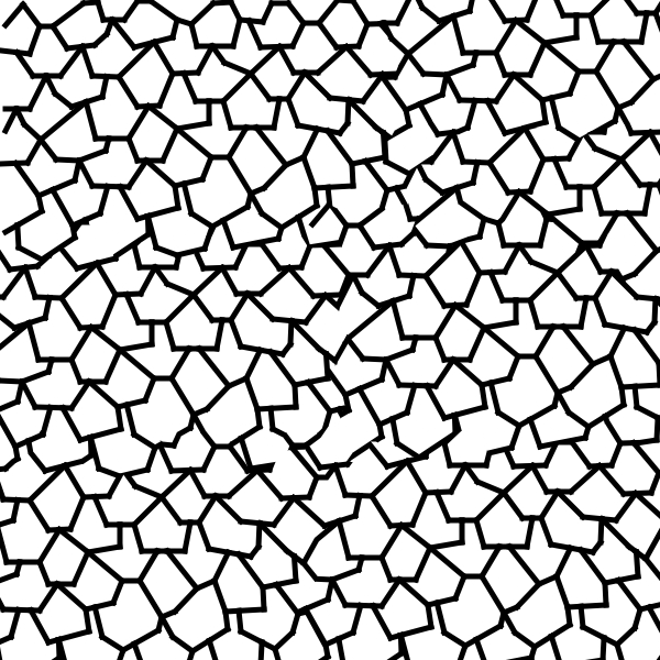
(f)

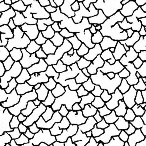
(g)

(h)

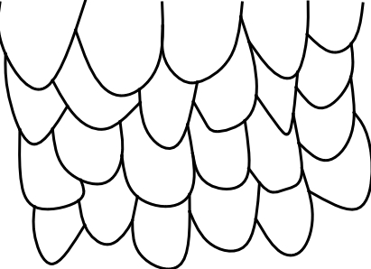
(i)

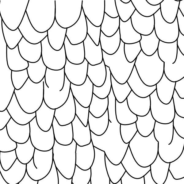
(j)

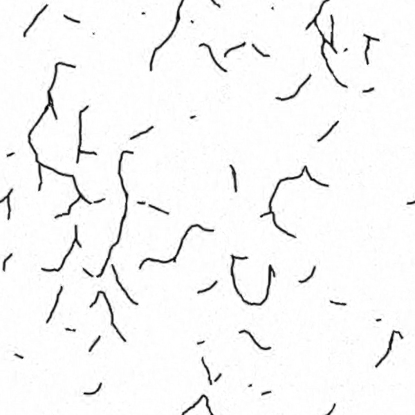
(k)

(l)

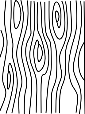
(m) Exemplar

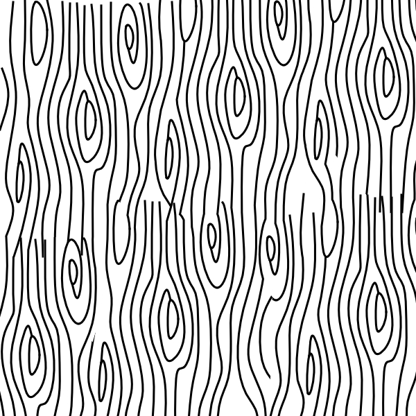
(n) [Cornet and Rouquier, 2004]

(o) [Wei, 2016]

(p) Ours

Figure 19. Comparison of our algorithm to texture synthesis. Texture synthesis methods need additional vector-pixel conversions and need to process all pixels instead of just samples around patterns.

Figure 19 shows the texture synthesis results by graph cut [Kwatra et al., 2003] (using the implementation in the GIMP Texturize Plugin [Cornet and Rouquier, 2004]) and multi-resolution patch-match (using the implementation in [Wei, 2016] with guidance channels [Kaspar et al., 2015]). As shown, pixel-based texture synthesis might not preserve continuous structures as well as our vector-based method. These methods also need additional vector-pixel conversions and need to process all pixels instead of just samples around patterns. If standard texture synthesis methods are applied for vector patterns, the rasterization, synthesis, and vectorization process can introduce extra quality degradation and computation overhead, and thus might not be practical for interactive authoring as we present in the supplementary video.