Exact real-time longitudinal correlation functions
of the massive XXZ chain

Abstract

We apply a recently developed thermal form factor expansion method to evaluate the real-time longitudinal spin-spin correlation functions of the spin-$\frac{1}{2}$ XXZ chain in the antiferromagnetically ordered regime at zero temperature. An analytical result incorporating all types of excitations in the model is obtained, without any approximations. This allows for the accurate calculation of the real-time correlations in this strongly interacting quantum system for arbitrary distances and times.

Dynamical correlation functions relate experimental observables like structure factors and transport coefficients to the microscopic details of quantum many-body systems. They are notoriously hard to calculate as they simultaneously probe all time and length scales. A particular class of many-body systems are integrable one-dimensional (1d) systems with short-range interactions. Due to the existence of a large number of local conserved quantities, they exhibit a peculiar phenomenology: they do not relax to a thermal equilibrium and can possess spin and charge currents which do not fully decay in time. These unusual properties are not only of fundamental interest but can be observed in experiments on systems which are almost integrable. This includes realizations of the 1d Bose gas in which quench dynamics as well as dynamical correlations in equilibrium have been studied [1, 2, 3, 4, 5]. The Heisenberg chain can be realized using cold atomic gases in optical lattices giving direct access to the spin dynamics in the spatio-temporal domain and to spin transport phenomena [6, 7, 8, 9]. Good realizations of the Heisenberg chain also occur as sub-structures in solid state systems [10, 11, 12]. Here they provide access to response functions in the momentum-frequency domain as, for example, the dynamical spin-structure factor (DSF) [13]. They also allow for the direct measurement of transport coefficients [14, 15, 16, 17]. Recent attempts to devise a general description of 1d close-to-integrable systems resulted in interesting phenomenological theories like the non-linear Luttinger liquid [18, 19, 20, 21, 22] or generalized hydrodynamics [23, 24, 25, 26, 27]. It is highly desirable to underpin such new phenomenologies with microscopic calculations. We note, moreover, that dynamical correlation functions in cold atomic gases can now be tested at time scales which are beyond the reach of modern numerical techniques. An exact calculation of dynamical correlation functions of 1d integrable models is therefore important for our understanding of state-of-the-art experiments. At the same time, it provides benchmarks for phenomenological theories and numerical methods.

Exact results on correlation functions are rather rare, even in low dimensions, and are mostly related to models belonging to the Free Fermion (FF) category [28]. For the Ising model in the scaling limit, a remarkable link to the Painlevé equations was established [29]. Dynamical correlations were studied for the XY model [30] and interesting phenomena of thermalization were addressed. An important next step was to go beyond FF and deal exactly with interacting systems. The vertex operator approach (VOA) opened up a new avenue to do so based on form factor expansions [31]. The evaluation of the two- and four-spinon contributions to the transverse DSF of the massive XXZ chain [32, 33, 34] and of the four-spinon contribution in the XXX limit [35] were important outcomes of this method. The complexity of the resultant multiple integrals has, however, hindered any further analysis. A hidden FF structure in the XXZ model was unveiled in Refs. [36, 37], and its remarkable outcome, the fermionic basis, yields exact correlation functions up to considerably large distances [38, 39]. The application of this method, however, has been limited to the static case so far. The quantum inverse scattering method (QISM) provides a complementary approach [40, 41], based on a determinant formula for the scalar product of on- and off-shell Bethe vectors [42]. Under restrictions on the possible excitations, it successfully reproduces the asymptotic correlation functions [43, 44] predicted by conformal field theory (CFT) [45]. Yet, in order to recover the DSF for the full range of frequencies and momenta, bound states must be taken into account, which are neglected in the CFT limit [46].

In this Letter we employ a recently developed [47, 48] form factor expansion for real-time correlation functions in equilibrium and obtain a simple, explicit, closed-form expression including all orders of excitations. We consider the XXZ chain with Hamiltonian

$$H\!=\!J\sum_{j=1}^{L}\Bigl{\{}\sigma_{j-1}^{x}\sigma_{j}^{x}+\sigma_{j-1}^{y}\sigma_{j}^{y}+\Delta\sigma_{j-1}^{z}\sigma_{j}^{z}\Bigr{\}}-\frac{h}{2}\sum_{j=1}^{L}\sigma_{j}^{z}$$ (1)

for length $L\to\infty$. Here $\sigma^{\alpha}_{j}$ are Pauli matrices, and $J>0$ is the exchange constant. We restrict ourselves to the antiferromagnetically ordered regime, characterized by values $\Delta=\cosh(\gamma)>1$ of the anisotropy and by magnetic fields in the range $0<h<4J\sinh(\gamma)\vartheta^{2}_{4}(0|q)$. Here we have set $q={\rm e}^{-\gamma}$, and the $\vartheta_{a}$ denote elliptic theta functions [49]. The special functions appearing here and below are summarized in the Suppl. Mat. [50].

In the antiferromagnetically ordered regime, the one-body properties of the elementary excitations are characterized by

$$p(\theta) =\frac{\pi}{2}+\theta-i\ln\biggl{(}\frac{\vartheta_{4}(\theta+i\gamma/2|q^{2})}{\vartheta_{4}(\theta-i\gamma/2|q^{2})}\biggr{)},$$ (2)

$$\varepsilon(\theta) =\frac{h}{2}-2J\sinh(\gamma)\vartheta_{3}(0|q)\vartheta_{4}(0|q)\frac{\vartheta_{3}(\theta|q)}{\vartheta_{4}(\theta|q)},$$ (3)

where $p(\theta)$ is the dressed momentum, $\varepsilon(\theta)$ the dressed energy and $\theta$ the rapidity of the quasiparticle. The interaction between excitations is described by the soliton scattering matrix,

$$S(\theta)={\rm e}^{i(\frac{\pi}{2}+\theta)}\frac{\Gamma_{q^{4}}\bigl{(}1+\frac{i\theta}{2\gamma}\bigr{)}\Gamma_{q^{4}}\bigl{(}\frac{1}{2}-\frac{i\theta}{2\gamma}\bigr{)}}{\Gamma_{q^{4}}\bigl{(}1-\frac{i\theta}{2\gamma}\bigr{)}\Gamma_{q^{4}}\bigl{(}\frac{1}{2}+\frac{i\theta}{2\gamma}\bigr{)}},$$ (4)

where $\Gamma_{q}$ denotes the $q$-gamma function. Due to the Yang-Baxter integrability of the model, any multi-particle scattering can be reduced to multiple two-body scattering events. One then naturally expects that correlation functions can be described solely by (2)-(4). We will show that an all-order expansion of the longitudinal dynamical correlation functions can indeed be described by these physical quantities with supplemental special functions of the $q$-gamma function family.

Our framework combines the QISM and the quantum transfer matrix (QTM) method [54, 55, 56]. The latter has been devised for the investigation of finite temperature bulk quantities and static correlation functions [57, 58]. It was generalized in [47], inspired by [59], to obtain form factor expansions of dynamical correlations at finite temperatures. We thus call it the thermal form factor expansion method. It has been successfully applied to the analysis of a FF model, the XX model [47, 60].

Although we are interested in the dynamical correlations in the ground state, we start from finite temperatures and consider the limits $h,T\rightarrow 0$. This may look redundant at first, but there are advantages of this approach. It is well known that the diagonalization of the Hamiltonian leads to string excitations of various lengths [61, 62, 63]. These are solutions of the Bethe ansatz equations which form regular patterns (‘strings’) in the complex plane for $L\rightarrow\infty$. Some quantities which characterize the correlations become singular if they are evaluated at the ideal string positions, e.g., $S(\pm i\gamma)$. The variety of string excitations and singularities leads to serious technical difficulties. The VOA provides an alternative description, free from string excitations, but its answer suffers from the high intricacy of multiple integrals. On the other hand, the QTM method, based on a mapping of the 1d quantum system to a two-dimensional classical system, does not directly deal with the Hamiltonian but rather with a transfer matrix acting in an auxiliary space. The possible excitations are thus different from those in the Hamiltonian basis. A previous study, using the higher level Bethe ansatz equations, concludes that only simple excitations are possible for $L\rightarrow\infty$ and $h,T\rightarrow 0$ with the limit $T\to 0$ taken first [64]. Their distribution in the complex rapidity plane can be interpreted as particle-hole excitations. A rapidity $y_{j}$ of a particle excitation is situated on a curve located above $[-\pi/2;\pi/2]$ such that ${\rm Im}\,y_{j}\sim\frac{\gamma}{2}$, while a hole rapidity $x_{j}$ is located below and ${\rm Im}\,x_{j}\sim-\frac{\gamma}{2}$. These excitations are not 2 strings since $\Re(y_{j}-x_{l})$ is generically non-zero and $\Im(y_{j}-x_{l})$ does not approach $\gamma$, even for $L\rightarrow\infty$. Thus, the QTM excitations do not produce the aforementioned singularities.

For the longitudinal correlation functions

$$\langle\sigma^{z}_{1}(t)\sigma^{z}_{m+1}(0)\rangle=\lim_{T\to 0}\mbox{tr}\,\{\sigma^{z}_{1}(t)\sigma^{z}_{m+1}(0)\exp(-H/T)\}/Z$$ (5)

where $Z$ is the partition function, the relevant excited states consist of an equal number of particles and holes. Thus, the resultant form factor expansion involves a sum over $\ell$, the number of particles and holes, and a sum over their possible locations. The higher level Bethe ansatz analysis shows that they obey a one-body equation for $T\rightarrow 0$. The sum over the possible locations is then replaced by simple integrations [50],

$$G(m,t):=\langle\sigma_{1}^{z}(t)\sigma_{m+1}^{z}(0)\rangle-(-1)^{m}\Bigl{(}\frac{\vartheta_{1}^{\prime}(0|q)}{\vartheta_{2}(0|q)}\Bigr{)}^{2}$$

$$=\!\sum_{\begin{subarray}{c}\ell\geq 1\\ k=0,1\end{subarray}}\!\frac{(-1)^{km}}{(\ell!)^{2}}\!\int_{C_{-}}\!\frac{d^{\ell}x}{(2\pi)^{\ell}}\!\int_{C_{+}}\!\frac{d^{\ell}y}{(2\pi)^{\ell}}{\rm e}^{-i\sum_{j=1}^{\ell}(mp(x_{j})-\varepsilon(x_{j})t)}$$

$$\phantom{ccc}\times{\rm e}^{i\sum_{j=1}^{\ell}(mp(y_{j})-\varepsilon(y_{j})t)}{\cal A}^{zz}(\{x_{i}\}_{i=1}^{\ell},\{y_{j}\}_{j=1}^{\ell}|k)$$ (6)

$$=\sum_{\ell\geq 1}I_{\ell}(m,t).$$

The integer $k\in\{0,1\}$ labels the degenerate ground states and we have subtracted the contribution of the staggered magnetization. There is some freedom to choose the contours $C_{\pm}$: the simplest choice is to take straight segments of length $\pi$ whose imaginary parts are $\pm\gamma/2+\delta$ where $\delta$ is positive. We will discuss the optimal choice of the contours for a numerical evaluation later.

The main purpose of the present report is to present the explicit form of ${\cal A}^{zz}$. It consists of determinants of two ${\ell}\times{\ell}$ matrices $\mathcal{M}$ and $\hat{\mathcal{M}}$ and a scalar part. For a compact presentation, we will use the shorthand notations

$$P_{j}={\rm e}^{2iy_{j}},\quad H_{j}={\rm e}^{2ix_{j}},\qquad 1\leq j\leq\ell,$$

and introduce the basic hypergeometric series [49, 65],

$$\Phi_{1}(P_{j})=\phantom{}_{2\ell}\Phi_{2\ell-1}\left({q^{-2},\{q^{2}\frac{P_{j}}{P_{i}}\}_{i\neq j},\{\frac{P_{j}}{H_{i}}\}_{i=1}^{\ell}\atop\phantom{--}\{\frac{P_{j}}{P_{i}}\}_{i\neq j},\{q^{2}\frac{P_{j}}{H_{i}}\}_{i=1}^{\ell}};q^{4},q^{4}\right),$$

$$\Phi_{2}(P_{j},P_{i})=$$

$$\phantom{}{}_{2\ell}\Phi_{2\ell-1}\left({\!q^{6},\{q^{6}\frac{P_{i}}{P_{r}}\}_{r\neq i,j},q^{2}\frac{P_{i}}{P_{j}},\{q^{4}\frac{P_{i}}{H_{r}}\}_{r=1}^{\ell}\atop\{q^{4}\frac{P_{i}}{P_{r}}\}_{r\neq i,j},q^{8}\frac{P_{i}}{P_{j}},\{q^{6}\frac{P_{i}}{H_{r}}\}_{r=1}^{\ell}};q^{4},q^{4}\!\right).$$ (7)

They originate from sums of residues of the soliton $S$ matrix at a particular series of poles. We further introduce

$$r_{\ell}(P_{j},P_{i})\\ =\frac{q^{2}(1-q^{2})^{2}\frac{P_{i}}{P_{j}}}{(1-\frac{P_{i}}{P_{j}})(1-q^{4}\frac{P_{i}}{P_{j}})}\prod_{r=1}^{\ell}\frac{1-\frac{P_{i}}{H_{r}}}{1-q^{2}\frac{P_{i}}{H_{r}}}\prod_{r\neq i,j}^{\ell}\frac{1-q^{2}\frac{P_{i}}{P_{r}}}{1-\frac{P_{i}}{P_{r}}}$$ (8)

and conveniently write $\Psi_{2}(P_{j},P_{i})=r_{\ell}(P_{j},P_{i})\Phi_{2}(P_{j},P_{i})$. The matrix element $\mathcal{M}_{ij}$ is then given by

$$\mathcal{M}_{ij}=\delta_{ij}D_{ij}+(1-\delta_{ij})E_{ij}$$ (9)

with

$$D_{ij} =\overline{\Phi}_{1}(P_{j})-{\Phi}_{1}(P_{j})(-1)^{k}\prod_{r=1}^{\ell}\frac{S(y_{j}-y_{r})}{S(y_{j}-x_{r})},$$ (10)

$$E_{ij} =-\overline{\Psi}_{2}(P_{j},P_{i})+{\Psi}_{2}(P_{j},P_{i})(-1)^{k}\prod_{r=1}^{\ell}\frac{S(y_{i}-y_{r})}{S(y_{i}-x_{r})}.$$

Here we define for any function $g(P_{1},\cdots,H_{1},\cdots)$,

$${\bar{g}}(P_{1},\cdots,H_{1},\cdots):=g(P_{1}^{-1},\cdots,H_{1}^{-1},\cdots).$$

The matrix element $\hat{\mathcal{M}}_{ij}$ is obtained from $\mathcal{M}_{ij}$ by replacing all $y_{r}\leftrightarrow-x_{r}$. Then ${\cal A}^{zz}$ is explicitly represented as

$${\cal A}^{zz}={\rm det}(\mathcal{M})\,{\rm det}(\hat{\mathcal{M}})\Bigl{(}\frac{\mu^{\ell}\vartheta^{\prime}_{1}(0|q)\sin{\cal P}}{\vartheta_{1}(\Sigma|q)}\Bigr{)}^{2}\\ \times\frac{\prod_{1\leq i<j\leq{\ell}}\psi_{D}(x_{i}-x_{j})\psi_{D}(y_{i}-y_{j})}{\prod_{i,j}\psi_{D}(x_{i}-y_{j})}.$$ (11)

We set ${\cal P}=\frac{\pi k}{2}+\sum_{l}\frac{p(y_{l})-p(x_{l})}{2}$, $\Sigma=-\frac{\pi k}{2}+\sum_{l}\frac{y_{l}-x_{l}}{2}$,

$$\psi(\theta)=\Gamma_{q^{4}}\bigl{(}\frac{1}{2}-\frac{i\theta}{2\gamma}\bigr{)}\Gamma_{q^{4}}\bigl{(}1-\frac{i\theta}{2\gamma}\bigr{)}\frac{G^{2}_{q^{4}}\bigl{(}1-\frac{i\theta}{2\gamma}\bigr{)}}{G^{2}_{q^{4}}\bigl{(}\frac{1}{2}-\frac{i\theta}{2\gamma}\bigr{)}},$$ (12)

and $\psi_{D}(\theta)=\vartheta^{2}_{1}(\theta|q^{2})\psi(\theta)\psi(-\theta)$. The symbol $G_{q}$ stands for the $q$-Barnes’ $G$ function. The overall constant $\mu$ is given by $\vartheta^{\prime}_{1}(0|q^{2})\psi(0)$.

We stress again that the compact formula (11) is valid for arbitrary ${\ell}$ and is free from any approximations. A similar all order formula has been derived for a quantum field theoretical model in Ref. [66] but so far not for lattice models. As an analytic benchmark, we can show that Eq. (11) for $\ell=1$ successfully reproduces [48] the result of the VOA for two spinons [67]. Generally, there is a conjecture [68] about the equivalence of the contributions from $2{\ell}$-spinons and from ${\ell}$-particle/hole excitations, which will be analyzed in detail in a separate publication.

Our main result (11) is very efficient for the numerical evaluation of the real-time dynamics. It allows us to obtain $G(m,t)$ for arbitrary distances and times, thus going far beyond of what can be achieved by purely numerical algorithms. In Ref. [68] the static correlation functions were investigated within the same framework, but using a Fredholm determinant representation for ${\cal A}^{zz}$. This inevitably included a numerical discretization approximation [69]. Although the results seem highly precise, it is important to check them independently as the actual evaluation involves numerical integrations. In the static case, we can establish results with high precision by a relatively small number of sampling points $n_{p}$ for $2{\ell}$ multiple integrations, see Table 1.

$\Delta$	$1.1$	$1.3$
$I_{1}(2,0)$	$0.2297348$	$0.2357141$
$I_{2}(2,0)$	$3.913377\times 10^{-2}$	$6.978269\times 10^{-3}$
$I_{3}(2,0)$	$1.614912\times 10^{-3}$	$2.120959\times 10^{-5}$
$(I_{1}+I_{2}+I_{3})$/exact	0.99951	0.999998

Table 1: Contributions to the static correlation $G(2,0)$ from small ${\ell}$ excitations for $\Delta=1.1,\,1.3$. The last row shows the ratios of the sums of the first three terms in Eq. (6) and the exact values [70], demonstrating that keeping only excitations with $\ell\leq 3$ already leads to highly accurate results.

Once the system starts to evolve in time, however, the numerical difficulty rapidly increases and it becomes necessary to replace the numerical estimation of the Fredholm determinants by an analytic one. To assess the accuracy of a truncated thermal form factor expansion in the dynamic case, we compare results based on the $\ell\leq 3$ contributions with data obtained by a time-dependent density matrix renormalization group algorithm (tDMRG) [71] in Fig. 1. The plots clearly indicate the importance of including not just the $\ell=1$ but also at least the $\ell=2$ contribution to obtain results which agree with the tDMRG data on this scale.

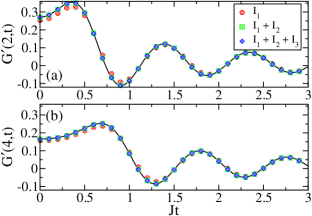
Figure 1: The real part $G^{\prime}(m,t)\equiv\Re G(m,t)$ for $\Delta=1.2$ with (a) $m=2$, and (b) $m=4$: Contributions of a thermal form factor expansion (symbols) are compared to tDMRG data (lines).

Based on this comparison, we restrict the following numerics to excitations up to $\ell=2$ and leave a more detailed discussion of the contributions of higher order excitations for a future study.

There are three asymptotic regimes, characterized by two critical velocities $v_{c_{1}}<v_{c_{2}}$ [72], or critical times $t_{c_{a}}=m/v_{c_{a}}\,(a=1,2)$. We talk of the space regime if $t<t_{c_{2}}$, the precursor regime if $t_{c_{2}}<t<t_{c_{1}}$, and the time regime if $t>t_{c_{1}}$. The qualitative differences between the regimes can be better seen for larger $m$. This is immediately handled by the form factor expansion approach since $m$ enters as a mere parameter. The correlation functions stay largely flat in the space regime, see Fig. 2. Towards the edge of the regime, there occurs an enhancement. After a transient behavior in the precursor regime, the correlation exhibits an oscillatory behavior.

Figure 2: The real part $G^{\prime}(m,t)$ for different $m$ and $\Delta=1.2$. The dashed lines indicate the critical times $Jt_{c_{1}}$ and $Jt_{c_{2}}$. For $\Delta\rightarrow 1$, $t_{c_{1}}\rightarrow t_{c_{2}}$ so there exists only an extremely narrow precursor regime (not visible on this scale) for $\Delta=1.2$.

Let us now briefly discuss some technical issues in evaluating Eq. (6). In the time regime, the phase factors can lead to serious numerical instabilities. The ordinary strategy to overcome this problem is to deform the integration contours, making them locally identical to the steepest descendent paths (SDP). This, however, does not work naively in the present case, since the SDPs for particles and holes intersect which leads to kinematic poles due to $\psi_{D}(y_{j}-x_{i})$ in the denominator of Eq. (11). To solve this problem, we take advantage of the QTM formulation: we return to finite temperatures and rewrite the formula in such a way that the contribution from the intersecting part is multiplied by the exponentially small factor ${\rm e}^{-1/T}$. Thus, in the zero temperature limit, one can neglect contributions from the kinematic poles. As a result, the two contours become disentangled and can be treated separately.

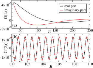
Figure 3: (a) $G(1,t)$ at long times for $\Delta=1.2$. (b) Comparison of $G^{\prime}(2,t)$ obtained by using the form factor expansion (symbols) with the two-spinon asymptotics (line) for $\Delta=1.4$.

Thanks to this trick, stable calculations at long times become possible, see Fig. 3(a). As a further test in the time regime, we compare in Fig. 3(b) our results to those obtained from the two-spinon term in a saddle point approximation [72], which is expected to be valid asymptotically in time. The predicted asymptotic behavior is given by $G(m,t)\sim{\rm e}^{i\omega t}/t$ for $m$ even with $\omega\sim J$.

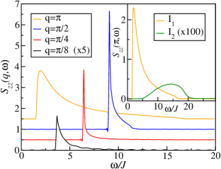
Figure 4: $S_{zz}(q,\omega)$ with $\Delta=2$ for various wave numbers $q$. Note that subsequent curves are shifted vertically by $0.5$. Inset: The $\ell=1$ contribution is non-zero only within the two-spinon continuum $[\omega_{\rm low},\omega_{\rm up}]$ while $\ell=2$ excitations contribute also for $\omega>\omega_{\rm up}$.

Finally, as a first application of (11), we evaluate the longitudinal DSF $S_{zz}(q,\omega)$, which is directly measurable in neutron scattering experiments. In contrast to $S_{+-}$ [32], the evaluation of $S_{zz}$ in the massive regime is technically difficult and the two-spinon result within the VOA has only recently been reported [73]. On the other hand, (6) and (11) allow to obtain the dynamical correlations for large $m$ and $t$, and we can readily perform a numerical Fourier transform. We subtract the contribution of the staggered magnetization and include both $\ell=1$ and $\ell=2$ excitations. The case $\Delta=2$ is plotted in Fig. 4 showing that the lineshapes as well as the weights for small $q$ are well resolved. We have checked that the sum rules [74] are satisfied with good accuracy. The $\ell=1$ excitations are constraint to the spinon energy band with lower and upper boundaries [32] $\omega_{\rm low}\sim 9.06J,\,\omega_{\rm up}\sim 11.76J\,(q=\pi/2)$ and $\omega_{\rm low}\sim 1.56J,\,\omega_{\rm up}\sim 16.56J\,(q=\pi)$, respectively. Higher $\ell$ excitations lead to a high-frequency tail which becomes more prominent for $\Delta\to 1$ [75]. For larger $\Delta$, the peaks will shift to larger $\omega$ and have smaller amplitudes. For $T\ll 1$, the line shape only weakly depends on the magnetic field if it is smaller than the lower critical field, in sharp contrast to the massless case ($|\Delta|<1$).

To summarize, we have presented a closed-form expression, incorporating all orders of particle-hole excitations, for the dynamical longitudinal correlation functions of the massive XXZ chain. This result opens up a new avenue to understand the dynamical response of strongly interacting quantum systems and is directly relevant for recent experiments on cold atomic gases. It does also provide a benchmark for the development of numerical algorithms including, for example, recent attempts to learn quantum dynamics using neural networks [76]. We note, furthermore, that the isotropic Heisenberg model, $\Delta=1$ in Eq. (1), is immediately obtained by rescaling all rapidities $x_{j},y_{j}$ by $\gamma x_{j},\gamma y_{j}$ and by taking $\gamma\rightarrow 0$. As all $I_{\ell}$ contribute with equal weight to the long-time asymptotic behavior, the explicit formula (11) will be an indispensable tool to study this limit in detail. Extensions to finite temperatures are promising and explicit expressions are already available from thermal form factor expansions if $T/J\ll 1$ [48]. Further progress in dealing with the kinematic poles along the lines of Ref. [60] is expected and will make it possible to access higher temperatures. A detailed analysis of the dynamical structure factor will also be an important subject of future studies.

In this supplement we provide some background material and a sketch of the derivation of our main result, Eq. (10) of the main text. The starting point will be our recent work [1].

I List of special functions

As the main result necessarily includes many special functions, we find it convenient to summarize their definitions. The basic ingredients of their definitions are the (multi-) $q$-Pochhammer symbols which, for $|q_{j}|<1$ and $a\in{\mathbb{C}}$, are defined as

$$(a;q_{1},\dots,q_{p})_{\infty}=\prod_{n_{1},\dots,n_{p}=0}^{\infty}(1-aq_{1}^{n_{1}}\dots q_{p}^{n_{p}}).$$ (S1)

We will often drop $\infty$ in the subscript. Based on this definition we introduce the $q$-gamma and $q$-Barnes functions $\Gamma_{q}$ and $G_{q}$,

$$\Gamma_{q}(x)=(1-q)^{1-x}\frac{(q;q)}{(q^{x};q)},\quad G_{q}(x)=(1-q)^{-\frac{1}{2}(1-x)(2-x)}(q;q)^{x-1}\frac{(q^{x};q,q)}{(q;q,q)}.$$ (S2)

All functions needed for the presentation of the final result of [1] belong to the above $q$-gamma family.

We follow the definition of theta funtions in [2]. Their product forms, e.g., read

$$\vartheta_{1}(x|q) =2q^{\frac{1}{4}}\sin(x)\prod_{n=1}^{\infty}(1-q^{2n})(1-2q^{2n}\cos(2x)+q^{4n}), \vartheta_{3}(x|q) =\prod_{n=1}^{\infty}(1-q^{2n})(1+2q^{2n-1}\cos(2x)+q^{4n-2}),$$

$$\vartheta_{2}(x|q) =2q^{\frac{1}{4}}\cos(x)\prod_{n=1}^{\infty}(1-q^{2n})(1+2q^{2n}\cos(2x)+q^{4n}), \vartheta_{4}(x|q) =\prod_{n=1}^{\infty}(1-q^{2n})(1-2q^{2n-1}\cos(2x)+q^{4n-2}).$$ (S3)

Recall that the other theta functions are related to, say, $\vartheta_{4}$ by shifts of the arguments [2].

The $q$-gamma and theta functions are related through the second functional equation of the $q$-gamma function which may be written as

$$\frac{\vartheta_{4}(x|q)}{\vartheta_{4}(0|q)}=\frac{\Gamma_{q^{2}}^{2}\bigl{(}{\frac{1}{2}}\bigr{)}}{\Gamma_{q^{2}}\bigl{(}{\frac{1}{2}-\frac{ix}{\gamma}}\bigr{)}\Gamma_{q^{2}}\bigl{(}{\frac{1}{2}+\frac{ix}{\gamma}}\bigr{)}}.$$ (S4)

In our derivation of the explicit formula for the amplitudes, we shall encounter the basic hypergeometric series [6], defined by

$$\phantom{}_{r}\Phi_{s}\left(\begin{array}[]{@{}r}a_{1},a_{2},\cdots,a_{r}\\ b_{1},b_{2},\cdots,b_{s}\end{array};q,z\right)=\sum_{n=0}^{\infty}\frac{(a_{1},\cdots,a_{r};q)_{n}}{(b_{1},\cdots,b_{s},q;q)_{n}}\Bigl{(}(-1)^{n}q^{\frac{n(n-1)}{2}}\Bigr{)}^{s+1-r}z^{n},$$ (S5)

where we have used the following standard notation for $q$-Pochhammer symbols,

$$(a;q)_{l}=\prod_{n=0}^{l-1}(1-aq^{n}),\quad(a_{1},a_{2},\cdots,a_{k};q)_{l}=(a_{1};q)_{l}(a_{2};q)_{l}\cdots(a_{k};q)_{l}.$$ (S6)

By definition $\phantom{}{}_{r}\Phi_{s}$ is invariant under permutations of the elements of the sets $\{a_{j}\}_{j=1}^{r}$ and $\{b_{j}\}_{j=1}^{s}$. In case that they can be split into disjoint subsets, say, $\{a_{j}\}_{j=1}^{r}=\{a^{(1)}_{j}\}_{j=1}^{l_{1}}\cup\{a^{(2)}_{j}\}_{j=1}^{l_{2}}\cup\cdots$, in place of (S5), we use a short-hand representation as employed in $\Phi_{1}$ and $\Phi_{2}$ in the main text,

$$\phantom{}{}_{r}\Phi_{s}\left(\begin{array}[]{@{}r}\{a^{(1)}_{j}\}_{j=1}^{l_{1}},\{a^{(2)}_{j}\}_{j=1}^{l_{2}},\cdots\\ \{b^{(1)}_{j}\}_{j=1}^{l^{\prime}_{1}},\{b^{(2)}_{j}\}_{j=1}^{l^{\prime}_{2}},\cdots\end{array};q,z\right).$$ (S7)

II QTM approach to dynamical correlation functions

Following the general strategy of the classical-to-quantum correspondence, we represent the correlation functions of the XXZ spin chain in terms of the correlation functions of an inhomogeneous six-vertex model. The vertical direction in the vertex model corresponds to discretized time and inverse temperature. We use a discretization scheme with $2N+2$ time and temperature slices proposed in [9] and combine it with a thermal form factor expansion [3, 7]. We refer to $N$ as the Trotter number. It should be sent to infinity at the end of calculation (the Trotter limit). This is a necessary procedure in order to recover the original continuous time quantum system at finite temperature $T$. The column-to-column transfer matrix acting on $2N+2$ sites is called the (dynamical) quantum transfer matrix (QTM).

For the formal definition of the inhomogeneous six-vertex model we have to introduce its weights. They are encoded in the $R$-matrix

$$\begin{array}[]{cc}R(\lambda,\mu)=\begin{pmatrix}1&0&0&0\\ 0&b(\lambda,\mu)&c(\lambda,\mu)&0\\ 0&c(\lambda,\mu)&b(\lambda,\mu)&0\\ 0&0&0&1\end{pmatrix},&\begin{array}[]{c}b(\lambda,\mu)=\frac{\sin(\mu-\lambda)}{\sin(\mu-\lambda+i\gamma)}\\[8.61108pt] c(\lambda,\mu)=\frac{\sin(i\gamma)}{\sin(\mu-\lambda+i\gamma)}\end{array}\end{array},$$ (S8)

where $\gamma>0$ is the same parameter as in $\Delta=\cosh(\gamma)$ and in $q={\rm e}^{-\gamma}$.

Using (S8) we define a staggered, twisted and inhomogeneous monodromy matrix acting on ‘vertical spaces’ with ‘site indices’ $1,\dots,2N+2$, and on a ‘horizontal space’ indexed $a$,

$$T_{a}(\lambda|h)={\rm e}^{h\sigma_{a}^{z}/2T}R_{2N+2,a}^{t_{1}}(\xi_{2N+2},\lambda+i\gamma/2)R_{a,2N+1}(\lambda+i\gamma/2,\xi_{2N+1})\dots R_{2,a}^{t_{1}}(\xi_{2},\lambda)R_{a,1}(\lambda+i\gamma/2,\xi_{1}).$$ (S9)

The superscript $t_{1}$ denotes transposition with respect to the first space on which $R$ is acting, and $\xi_{1},\dots,\xi_{2N+2}$ are $2N+2$ complex ‘inhomogeneity parameters’. We fix these parameters to the values [7, 9]

$$\xi_{2j-1}=-\xi_{2j}=\begin{cases}-\frac{it}{\kappa N}&j=1,\dots,\frac{N}{2}\\[2.15277pt] \epsilon&j=\frac{N}{2}+1\\[4.30554pt] \frac{it+1/T}{\kappa N}&j=\frac{N}{2}+2,\dots,N+1,\end{cases}$$ (S10)

where $1/\kappa=-2iJ\sinh(\gamma)$ and $\epsilon\neq 0$ is a regularization parameter.

By construction, the monodromy matrix $T_{a}(\lambda|h)$ can be seen as a $2\times 2$ matrix in space $a$, corresponding to a lattice site in the spin chain, with entries $A(\lambda|h),\dots,D(\lambda|h)$ that are operators acting on a $2^{2N+2}$ dimensional auxiliary space,

$$T_{a}(\lambda|h)=\begin{pmatrix}A(\lambda|h)&B(\lambda|h)\\ C(\lambda|h)&D(\lambda|h)\end{pmatrix}_{a}.$$ (S11)

Thanks to the solution of the inverse problem, any local spin operators in dynamical correlation functions are expressible in terms of these operators. The QTM $\tau(\lambda|h)$ and its twisted version $\tau(\lambda|h^{\prime})$ are defined by

$$\tau(\lambda|h)={\text{t}r}_{a}T_{a}(\lambda|h)=A(\lambda|h)+D(\lambda|h),\qquad\tau(\lambda|h^{\prime})={\rm e}^{\alpha\gamma}A(\lambda|h)+{\rm e}^{-\alpha\gamma}D(\lambda|h),$$ (S12)

where the twist angle $\alpha$ is absorbed into the shift, $\frac{h^{\prime}}{2T}=\frac{h}{2T}+\alpha\gamma$, see (S9).

We denote the eigenvalues and eigenstates of the QTM by $\Lambda_{n}(\lambda|h)$ and $|n,h\rangle$. Since $\tau(\lambda|h)$ is non-Hermitian, its eigenvalues are generally not all real. Still, there is a unique eigenstate $|0,h\rangle$, whose eigenvalue is real and of largest modulus. We call this state the dominant state. For brevity we shall suppress the suffix ‘0’ and write $\Lambda(\lambda|h)$ and $|h\rangle$ in this case.

Let us define $\Sigma^{z}(\lambda|h)$, which is related to the spin operator $\sigma^{z}$ and has a simple relation with $\tau(\lambda|h,\alpha)$,

$$\Sigma^{z}(\lambda|h)=A(\lambda|h)-D(\lambda|h)=\left.\partial_{\alpha\gamma}\tau(\lambda|h^{\prime})\right|_{\alpha=0}.$$ (S13)

We introduce an important object by using $\Sigma^{z}(\lambda|h)$,

$$A_{n}^{zz}(h)=\frac{\langle h|\Sigma^{z}(-i\gamma/2|h)|n,h\rangle\langle n,h|\Sigma^{z}(-i\gamma/2|h)|h\rangle}{\Lambda_{n}(-i\gamma/2|h)\langle h|h\rangle\Lambda(-i\gamma/2|h)\langle n,h|n,h\rangle},$$ (S14)

which will turn into ${\cal A}_{zz}$ in the end.

The longitudinal correlation function can then be represented as [7]

$$\bigl{\langle}\sigma_{1}^{z}(t)\sigma_{m+1}^{z}\bigr{\rangle}_{T}=\lim_{N\rightarrow\infty}\lim_{\epsilon\rightarrow 0}\sum_{n}A_{n}^{zz}(h)\rho_{n}(-i\gamma/2|h)^{m}\biggl{(}\frac{\rho_{n}(-i\gamma/2-it/\kappa N|h)}{\rho_{n}(-i\gamma/2+it/\kappa N|h)}\biggr{)}^{\frac{N}{2}},$$ (S15)

where $\rho_{n}(\lambda|h)=\Lambda_{n}(\lambda|h)/\Lambda(\lambda|h)$.

By means of (S13) one can rewrite (S14) as

$$A_{n}^{zz}(h)=\left.\delta_{n,0}\biggl{(}\frac{\partial_{\alpha\gamma}\Lambda(-i\gamma/2|h)}{\Lambda(-i\gamma/2|h)}\biggr{)}^{2}\right|_{\alpha=0}+\frac{1}{2}\bigl{(}\partial^{2}_{\alpha\gamma}A_{n}(h,h^{\prime})\bigr{)}_{\alpha=0}\biggl{[}\rho_{n}(-i\gamma/2|h)-2+\rho_{n}(-i\gamma/2|h)^{-1}\biggr{]}$$ (S16)

where we have introduced

$$A_{n}(h,h^{\prime})=\frac{\langle h|n,h^{\prime}\rangle\langle n,h^{\prime}|h\rangle}{\langle h|h\rangle\langle n,h|n,h\rangle}$$ (S17)

and also used that $A_{n}(h,h)=0$ if $n\neq 0$.

III Summation, Trotter limit, and zero temperature limit

Equation (S15) gives us access to the longitudinal two-point function at any finite temperature. For the evaluation of its right hand side we have to proceed in three steps. 1.) Evaluate the amplitudes $A_{n}(h,h^{\prime})$ and eigenvalue ratios $\rho_{n}(\cdot|h)$ at finite Trotter number for all excited states. 2.) Sum up the series. 3.) Perform the Trotter limit.

A classification of all excited states at sufficiently low temperatures was achieved in [4]. If, at finite magnetic field $h$, the temperature is low enough, all excited states can be described as particle-hole excitations. All string excitations disappear from the spectrum. This made it possible to obtain all eigenvalue ratios $\rho_{n}(\cdot|h)$ in closed form in this limit. In our recent work [1] we attempted to use the same classification of the eigenstates to obtain explicit expressions for the amplitudes $A_{n}(h,h^{\prime})$ defined in (S17). Using Slavnov’s scalar product formula [10] the right hand side is expressed in terms of the sets of Bethe roots of the dominant and excited states which parameterize certain ‘Slavnov determinants’. Taking the Trotter limit of these determinants is not immediate and not a unique procedure. In the previous work [5] we obtained expressions for the amplitudes involving Fredholm determinants of certain integral operators that were valid in the low-$T$ limit. In our most recent work [1], inspired by [8], we obtained expressions that involved only determinants of finite matrices at low $T$. Here we only summarize the final result of [1] and refer to the paper for more details. Starting from the final result of [1] we can derive the fully explicit formula (10), reported in the Letter.

We first introduce the functions that characterize the amplitude in the Trotter limit and at $T=0$. These are the bare energy

$$e(\lambda)=\cot(\lambda)-\cot(\lambda-i\gamma)\,,\quad$$ (S18)

a function with a complex parameter $\alpha$

$$g_{\alpha}(\lambda,\mu)=\frac{\vartheta_{1}^{\prime}(0|q)\vartheta_{2}(\mu-\lambda-\alpha|q)}{\vartheta_{2}(\alpha|q)\vartheta_{1}(\mu-\lambda|q)},$$ (S19)

the ‘averaged shift function’

$$\Sigma_{0}=\frac{1}{2}\biggl{(}-k\pi+i\alpha\gamma+\sum_{j=1}^{\ell}(y_{j}-x_{j})\biggr{)},$$ (S20)

where the $y_{j}$ and $x_{j}$ are the particle and hole rapidities introduced in the main text, and a pair of ‘weight functions’ defined for $\sigma=\pm$ as

$$\Phi^{(\sigma)}(\lambda)={\rm e}^{\sigma i\Sigma_{0}}\prod_{j=1}^{\ell}\frac{\Gamma_{q^{4}}\Bigl{(}\frac{1}{2}-\frac{\sigma i(\lambda-x_{j})}{2\gamma}\Bigr{)}\Gamma_{q^{4}}\Bigl{(}1+\frac{\sigma i(\lambda-x_{j})}{2\gamma}\Bigr{)}}{\Gamma_{q^{4}}\Bigl{(}\frac{1}{2}-\frac{\sigma i(\lambda-y_{j})}{2\gamma}\Bigr{)}\Gamma_{q^{4}}\Bigl{(}1+\frac{\sigma i(\lambda-y_{j})}{2\gamma}\Bigr{)}}.$$ (S21)

They all enter in the definition of the key ingredients, $\Omega$ and $\overline{\Omega}$,

$$\Omega(\lambda,\mu) =g_{\Sigma_{0}}(\lambda,\mu)-\int_{-\pi/2}^{\pi/2}\frac{dz}{2\pi i}\frac{\Phi^{(-)}(\mu)}{\Phi^{(+)}(z)}\,g_{\Sigma_{0}}(\lambda,z)e(z-\mu),$$ (S22a)

$$\overline{\Omega}(\lambda,\mu) =g_{-\Sigma_{0}}(\lambda,\mu)-\int_{-\pi/2}^{\pi/2}\frac{dz}{2\pi i}\>\frac{\Phi^{(-)}(z)}{\Phi^{(+)}(\mu)}\,g_{-\Sigma_{0}}(\lambda,z)e(\mu-z).$$ (S22b)

Finally the thermal form factor expansion of the longitudinal correlation function as obtained in [1] reads

$$\langle\sigma_{1}^{z}(t)\sigma_{1+m}^{z}(0)\rangle=(-1)^{m}\frac{\vartheta_{1}^{\prime}(0|q)^{2}}{\vartheta_{2}(0|q)^{2}}\\ +\sum_{k=0,1}(-1)^{km}\sum_{\ell=1}^{\infty}\frac{1}{({\ell}!)^{2}}\int_{C_{-}}\frac{d^{\ell}x}{(2\pi)^{\ell}}\int_{C_{+}}\frac{d^{\ell}y}{(2\pi)^{\ell}}{\cal A}_{zz}(\{x\},\{y\}|k){\rm e}^{-i\sum_{j=1}^{\ell}\bigl{(}p(x_{j})m-\varepsilon(x_{j})t\bigr{)}}{\rm e}^{i\sum_{j=1}^{\ell}\bigl{(}p(y_{j})m-\varepsilon(y_{j})t\bigr{)}},$$ (S23)

where the amplitude ${\cal A}_{zz}(\{x\},\{y\}|k)$ takes the form

$${\cal A}_{zz}(\{x\},\{y\}|k)=(-1)^{\ell}4\sin^{2}\biggl{(}\frac{\pi k}{2}+\sum_{j=1}^{\ell}\frac{p(y_{j})-p(x_{j})}{2}\biggr{)}\frac{\vartheta^{2}_{2}(\Sigma_{0}|q)}{\vartheta^{2}_{2}(0|q)}\prod_{i,j=1}^{\ell}\frac{\psi(x_{i}-x_{j})\psi(y_{i}-y_{j})}{\psi(x_{i}-y_{j})\psi(y_{j}-x_{i})}\\ \times\left.\frac{\partial{\rm det}\,\Omega(x_{i},y_{j})}{\partial i\alpha\gamma}\frac{\partial{\rm det}\,\overline{\Omega}(x_{i},y_{j})}{\partial i\alpha\gamma}\right|_{\alpha=0}.$$ (S24)

IV The derivation of the explicit formula for the amplitude

We have to take the $\alpha$-derivatives explictly in (S24) to obtain the amplitudes ${\cal A}_{zz}$ that determine the physical correlation function. Each matrix element $\Omega(x_{i},y_{j})$ is calculated from (S22a) and (S22b), and the only $\alpha$ dependency appears through $\Sigma_{0}$. It is then easy to check that the column vectors or the row vectors of the matrix $\Omega$ are not simply parallel. As the existence of a null vector of $\Omega$ is proven [1], we can safely perform a Taylor expansion with respect to $\alpha$. It results, however, in a sum over many terms which is inconvenient for practical use. Thus, the first order zeros in $\alpha$ are better factored out explicitly from ${\rm det}\,\Omega$ and ${\rm det}\,\overline{\Omega}$.

The integral in (S22a) can be calculated by means of the residue theorem as the integrand is $\pi$-periodic and meromorphic. It has infinite series of simple poles in the upper and in the lower half plane. We obtain two different representations of $\Omega(x_{i},y_{j})$ by closing the integration contour in the upper or in the lower half plane. These representations can be neatly written in terms of special $\alpha$-dependent basic hypergeometric series,

$$\Phi_{1}\bigl{(}P_{j},\{P_{l}\}_{l\neq j},\{H_{r}\},\alpha\bigr{)} =\phantom{}_{2\ell}\Phi_{2\ell-1}\left(\begin{array}[]{@{}r}q^{-2},\{q^{2}\frac{P_{j}}{P_{l}}\}_{l\neq j},\{\frac{P_{j}}{H_{r}}\}_{r=1}^{\ell}\\ \{\frac{P_{j}}{P_{l}}\}_{l\neq j},\{q^{2}\frac{P_{j}}{H_{r}}\}_{r=1}^{\ell}\end{array};q^{4},q^{4}{\rm e}^{-2\alpha\gamma}\right),$$ (S25c)

$$\Phi_{2}\bigl{(}P_{j},P_{i},\{P_{l}\}_{l\neq i,j},\{H_{r}\},\alpha\bigr{)} =\phantom{}_{2\ell}\Phi_{2\ell-1}\left(\begin{array}[]{@{}r}q^{6},\{q^{6}\frac{P_{i}}{P_{l}}\}_{l\neq i,j},q^{2}\frac{P_{i}}{P_{j}},\{q^{4}\frac{P_{i}}{H_{r}}\}_{r=1}^{\ell}\\ \{q^{4}\frac{P_{i}}{P_{l}}\}_{l\neq i,j},q^{8}\frac{P_{i}}{P_{j}},\{q^{6}\frac{P_{i}}{H_{r}}\}_{r=1}^{\ell}\end{array};q^{4},q^{4}{\rm e}^{-2\alpha\gamma}\right),$$ (S25f)

$$\Phi_{3}\bigl{(}P_{j},H_{i},\{P_{l}\}_{l\neq j},\{H_{r}\}_{r\neq i},\alpha\bigr{)} =\phantom{}_{2\ell}\Phi_{2\ell-1}\left(\begin{array}[]{@{}r}q^{2},\frac{H_{i}}{P_{j}},\{q^{4}\frac{H_{i}}{P_{l}}\}_{l\neq j},\{q^{2}\frac{H_{i}}{H_{r}}\}_{r\neq i}\\ q^{6}\frac{H_{i}}{P_{j}},\{q^{2}\frac{H_{i}}{P_{l}}\}_{l\neq j},\{q^{4}\frac{H_{i}}{H_{r}}\}_{r\neq i}\end{array};q^{4},q^{4}{\rm e}^{-2\alpha\gamma}\right).$$ (S25i)

Here the variable set $\{*\}$ means that the function is invariant under permutations among the members of $*$. We will drop the symmetric arguments and use the abbreviations $\Phi_{1}(P_{j},\alpha)$, $\Phi_{2}(P_{j},P_{i},\alpha)$ or $\Phi_{3}(P_{j},H_{i},\alpha)$. We further set

$$\Psi_{2}(P_{j},P_{i},\alpha)={\rm e}^{-2\alpha\gamma}r_{\ell}(P_{j},P_{i})\Phi_{2}(P_{j},P_{i},\alpha),$$ (S26)

where $r_{\ell}$ is defined in Eq. (7) of the main text.

The calculation of the sum of the residues is straightforward but rather cumbersome. It finally results in

$$\Omega(x_{j},y_{i}) =-\frac{\Phi^{(-)}(y_{i})}{\Phi^{(+)}(y_{i})}g_{\Sigma_{0}}(x_{j},y_{i})\Phi_{1}(P_{i},\alpha)+\sum_{\begin{subarray}{c}l=1\\ l\neq i\end{subarray}}^{\ell}\frac{\Phi^{(-)}(y_{i})}{\Phi^{(+)}(y_{l})}g_{\Sigma_{0}}(x_{j},y_{l})\Psi_{2}(P_{i},P_{l},\alpha)$$

$$\mspace{489.0mu}+\frac{\Phi^{(-)}(y_{i})}{\Phi^{(-)}(x_{j})}e(y_{i}-x_{j})\Phi_{3}(P_{i},H_{j},\alpha),$$

$$=g_{\Sigma_{0}}(x_{j},y_{i})\overline{\Phi}_{1}(P_{i},\alpha)-\sum_{\begin{subarray}{c}l=1\\ l\neq i\end{subarray}}^{\ell}\frac{\Phi^{(-)}(y_{i})}{\Phi^{(-)}(y_{l})}g_{\Sigma_{0}}(x_{j},y_{l})\overline{\Psi}_{2}(P_{i},P_{l},\alpha)+\frac{\Phi^{(-)}(y_{i})}{\Phi^{(+)}(x_{j})}e(x_{j}-y_{i})\overline{\Phi}_{3}(P_{i},H_{j},\alpha).$$ (S27)

Slightly generalizing the definition in the main text the overbar means here that $H_{j}\rightarrow 1/H_{j}$, $P_{i}\rightarrow 1/P_{i}$, and $\alpha\rightarrow-\alpha$. The first equation is the result of closing the contour in the upper half plane, the second equation comes from closing the contour in the lower half plane.

Neither of the two expressions (S27) looks particularly useful, but they can be used to simplify one another. The key observation is that they have a simple dependence on the index $k$. It enters $\Omega$ only through $\Sigma_{0}$ (cf. Eq. (S20)). In order to make this dependence explicit we introduce

$$\sigma_{0}=\Sigma_{0}+\frac{\pi k}{2}$$ (S28)

which is independent of $k$. Then $\Phi^{(\pm)}(\lambda)=(-1)^{k}{\rm e}^{\pm i\sigma_{0}}\phi_{0}^{(\pm)}(\lambda)$, where $\phi_{0}^{(\pm)}(\lambda)$ is independent of $k$. The dependence of $g_{\Sigma_{0}}$ on $k$ is slightly more tricky to work out. Setting

$$\theta_{a}(w,\sigma_{0})=\frac{\vartheta_{a}(2\sigma_{0}-w|q^{2})}{\vartheta_{a}(w|q^{2})}$$ (S29)

for $a=1,4$ we see that

$$g_{\Sigma_{0}}(x,y)=-\theta_{1}^{\prime}(2\sigma_{0},\sigma_{0})\bigl{(}\theta_{1}(y-x,\sigma_{0})+(-1)^{k}\theta_{4}(y-x,\sigma_{0})\bigr{)}.$$ (S30)

Altogether, using these simple formulas, the two expressions for $\Omega$ take the form $\Omega(x_{j},y_{i})=(-1)^{k}A+B=(-1)^{k}C+D$, where $A$, $B$, $C$, $D$ are independent of $k$ and $A$, $B$ refer to the first equation in (S27), whereas $C$, $D$ refer to the second equation. While $A$ and $D$ have forms that are convenient for factorization, $B$ and $C$ do not. Thanks to the equality, however, it follows that $A=C$, $B=D$ and therefore $\Omega(x_{j},y_{i})=(-1)^{k}A+D$. That is, we can represent $\Omega$ entirely in terms of convenient expressions. Spelling this out explicitly we obtain

$$\Omega(x_{j},y_{i})=-\sum_{l=1}^{\ell}\biggl{\{}\delta_{il}\biggl{[}\overline{\Phi}_{1}(P_{i},\alpha)-\frac{\Phi^{(-)}(y_{i})}{\Phi^{(+)}(y_{i})}\Phi_{1}(P_{i},\alpha)\biggr{]}\\ -(1-\delta_{il})\biggl{[}\frac{\Phi^{(-)}(y_{i})}{\Phi^{(-)}(y_{l})}\overline{\Psi}_{2}(P_{i},P_{l},\alpha)-\frac{\Phi^{(-)}(y_{i})}{\Phi^{(+)}(y_{l})}\Psi_{2}(P_{i},P_{l},\alpha)\biggr{]}\biggr{\}}\theta_{1}^{\prime}(2\sigma_{0},\sigma_{0})\theta_{1}(y_{l}-x_{j},\sigma_{0})$$ (S31)

which is a matrix element of a product of two matrices. The factor $(-1)^{k}$, that appears at an intermediate stage, is re-absorbed in $\Phi^{(\pm)}$ here.

Thus,

$$\det\Omega(x_{j},y_{i})=(-1)^{\ell}\det\bigl{\{}\theta_{1}^{\prime}(2\sigma_{0},\sigma_{0})\theta_{1}(y_{l}-x_{j},\sigma_{0})\bigr{\}}\det\{\mathcal{M}(\alpha)\},$$ (S32)

where

$$\mathcal{M}(\alpha)_{ij}=\delta_{ij}\biggl{[}\overline{\Phi}_{1}(P_{j},\alpha)-\frac{\Phi^{(-)}(y_{j})}{\Phi^{(+)}(y_{j})}\Phi_{1}(P_{j},\alpha)\biggr{]}-(1-\delta_{ij})\biggl{[}\overline{\Psi}_{2}(P_{j},P_{i},\alpha)-\frac{\Phi^{(-)}(y_{i})}{\Phi^{(+)}(y_{i})}\Psi_{2}(P_{j},P_{i},\alpha)\biggr{]}.$$ (S33)

In the last step, we divide the $i$-th row by $\Phi^{(-)}(y_{i})$ and multiply the $l$-th column by $\Phi^{(-)}(y_{l})$, which leaves the determinant invariant.

The first determinant is of elliptic Cauchy (or Frobenius) type and can be calculated in product form,

$$\det\bigl{\{}\theta_{1}^{\prime}(2\sigma_{0},\sigma_{0})\theta_{1}(y_{i}-x_{j},\sigma_{0})\bigr{\}}=\frac{\vartheta_{1}(i\alpha\gamma|q^{2})}{\vartheta_{1}(2\sigma_{0}|q^{2})}\bigl{(}\vartheta_{1}^{\prime}(0|q^{2})\bigr{)}^{\ell}\,\frac{\prod_{1\leq j<r\leq\ell}\vartheta_{1}(x_{j}-x_{r}|q^{2})\vartheta_{1}(y_{r}-y_{j}|q^{2})}{\prod_{j,r=1}^{\ell}\vartheta_{1}(x_{j}-y_{r}|q^{2})}.$$ (S34)

Note that the prefactor is of order $\alpha$ here. This makes it easy to calculate the $\alpha$-derivative of $\det\Omega$ occurring on the right hand side of (S24),

$$\frac{\partial\det\Omega(x_{j},y_{i})}{\partial i\alpha\gamma}\biggr{|}_{\alpha=0}=(-1)^{\ell}\frac{\vartheta_{1}^{\prime}(0|q^{2})\bigl{(}\vartheta_{1}^{\prime}(0|q^{2})\bigr{)}^{\ell}}{\vartheta_{1}(\sum_{j}(y_{j}-x_{j})|q^{2})}\,\frac{\prod_{1\leq j<r\leq\ell}\vartheta_{1}(x_{j}-x_{r}|q^{2})\vartheta_{1}(y_{r}-y_{j}|q^{2})}{\prod_{j,r=1}^{\ell}\vartheta_{1}(x_{j}-y_{r}|q^{2})}\det\{\mathcal{M}(0)\}.$$ (S35)

A similar formula is obtained for the $\alpha$-derivative of $\det\overline{\Omega}$ if we take into account that

$$\overline{\Omega}(y_{j},x_{i})=-\left.\Omega(x_{j},y_{i})\right|_{x_{j}\rightarrow-y_{j},y_{i}\rightarrow-x_{i},\alpha\rightarrow\alpha}.$$ (S36)

Inserting the results for the derivatives of $\det\Omega$ and of $\det\overline{\Omega}$ back into (S24) and using a few standard theta function identities we arrive at Eqs. (5)-(11) of the main text.

References

- [1] C. Babenko, F. Göhmann, K. K. Kozlowski, and J. Suzuki, A thermal form factor series for the longitudinal two-point function of the Heisenberg-Ising chain in the antiferromagnetic massive regime, J. Math. Phys. 62, 041901 (2021).
- [2] E. T. Whittaker and G. N. Watson, A Course of Modern Analysis, fourth ed., ch. 21, Cambridge University Press (Cambridge, 1963).
- [3] M. Dugave, F. Göhmann, and K. K. Kozlowski, Thermal form factors of the XXZ chain and the large-distance asymptotics of its temperature dependent correlation functions, J. Stat. Mech.: Theor. Exp. (2013), P07010.
- [4] M. Dugave, F. Göhmann, K. K. Kozlowski, and J. Suzuki, Low-temperature spectrum of correlation lengths of the XXZ chain in the antiferromagnetic massive regime, J. Phys. A 48 (2015), 334001.
- [5] , Thermal form factor approach to the ground-state correlation functions of the XXZ chain in the antiferromagnetic massive regime, J. Phys. A 49 (2016), 394001.
- [6] G. Gasper and M. Rahman, Basic hypergeometric series, scd. ed., Encyclopedia of Mathematics and its Applications, vol. 96, Cambridge University Press, 2004.
- [7] F. Göhmann, M. Karbach, A. Klümper, K. K. Kozlowski, and J. Suzuki, Thermal form-factor approach to dynamical correlation functions of integrable lattice models, J. Stat. Mech.: Theor. Exp. (2017), 113106.
- [8] N. Kitanine and G. Kulkarni, Thermodynamic limit of the two-spinon form factors for the zero field XXX chain, SciPost Phys. 6 (2019), 076.
- [9] K. Sakai, Dynamical correlation functions of the XXZ model at finite temperature, J. Phys. A 40 (2007), 7523.
- [10] N. A. Slavnov, Calculation of scalar products of the wave functions and form factors in the framework of the algebraic Bethe ansatz, Teor. Mat. Fiz. 79 (1989), 232.