A Virgo Environmental Survey Tracing Ionised Gas Emission (VESTIGE).IX. The effects of ram pressure stripping down to the scale of individual HII regions in the dwarf galaxy IC 3476

Abstract

Context. We study the IB(s)m galaxy IC 3476 observed in the context of the Virgo Environmental Survey Tracing Ionised Gas Emission (VESTIGE), a blind narrow-band H$\alpha$+[NII] imaging survey of the Virgo cluster carried out with MegaCam at the CFHT. The deep narrow-band image reveals a very pertubed ionised gas distribution, characterised by a prominent banana-shaped structure in the front of the galaxy formed of giant HII regions crossing the stellar disc, with star forming structures at $\sim$ 8 kpc from the edges of the stellar disc, detected also in a deep FUV ASTROSAT/UVIT image. This particular morphology indicates that the galaxy is undergoing an almost edge-on ram pressure stripping event. The same H$\alpha$+[NII] image also shows that the star formation activity is totally quenched in the leading edge of the disc, where the gas has been removed during the interaction with the surrounding medium. The SED fitting analysis of the multifrequency data indicates that this quenching episode is very recent ($\sim$ 50 Myr), and roughly corresponds to an increase of the star formation activity by a factor of $\sim$ 161% in the inner regions with respect to what expected for secular evolution. The analysis of these data, whose angular resolution allows the study of the induced effects of the perturbation down to the scale of individual HII regions ($r_{\mathrm{eq}}$ $\simeq$ 40 pc), also suggests that the increase of the star formation activity is due to the compression of the gas along the stellar disc of the galaxy, which is able to increase its mean electron density and boost the star formation process producing bright HII regions with luminosities up to $L(H\alpha)$ $\simeq$ 10³⁸ erg s^-1. The combined analysis of the VESTIGE data with deep IFU spectroscopy gathered with MUSE and with high spectral resolution Fabry Perot data also indicates that the hydrodynamic interaction has deeply perturbed the velocity field of the ionised gas component while leaving unaffected that of the stellar disc. The comparison of the data with tuned high-resolution hydrodynamic simulations accounting for the different gas phases (atomic, molecular, ionised) consistently indicates that the perturbing event is very recent (50-150 Myr), once again confirming that ram pressure stripping is a violent phenomenon able to perturb on short timescales the evolution of galaxies in rich environments.

Aims.

Methods.

Results.

1 Introduction

Galaxies inhabiting rich environments are subject to different kind of perturbations that modify their evolution. In rich clusters, which are characterised by a hot ($T$ $\simeq$ 10⁷-10⁸ K) and dense ($\rho$ $\simeq$ 10^-3 cm^-3) intergalactic medium (IGM; e.g. Sarazin 1986), the hydrodynamic pressure exerted on the interstellar medium (ISM) of gas-rich members moving at high velocity ($\simeq$ 1000 km s^-1) can remove the gas and quench the activity of star formation of the perturbed galaxies. A lot of observational evidence, such as the presence of galaxies with long cometary tails in the different gas phases (atomic cold - e.g. Chung et al. 2007; ionised - Yagi et al. 2010; hot - e.g. Sun et al. 2007) without any associated stellar counterpart, or the high frequency of spirals with radially truncated gaseous discs (e.g. Cayatte et al. 1994; Koopmann & Kenney 2004), indicates that this process, which is commonly referred to as ram pressure stripping (Gunn & Gott 1972), dominates the evolution of gas-rich late-type systems in nearby massive clusters (e.g. Boselli & Gavazzi 2006, 2014).

While many representative objects undergoing a ram pressure stripping event have been already studied in detail using multifrequency observations (Kenney et al. 2004, 2014, 2015; Crowl et al. 2005; Boselli et al. 2016a; Sun et al. 2006, 2007, 2010; Merluzzi et al. 2013; Abramson & Kenney 2014; Abramson et al. 2011, 2016; Jachym et al. 2013, 2014, 2017, 219; Fumagalli et al. 2014; Fossati et al. 2016; Poggianti et al. 2019; Bellhouse et al. 2019; Deb et al. 2020; Moretti et al. 2020a) and tuned models and simulations (Vollmer et al. 1999, 2000, 2004a,b, 2006a, 2008a,b, 2012, 2018; Roediger & Hensler 2005; Boselli et al. 2006), we are still far from understanding the physics of this perturbing mechanism and the fate of the stripped gas once removed from the galaxy disc. The behaviour of galaxies undergoing ram pressure stripping might drastically change from object to object in a way still not totally predictable. Indeed, in some galaxies gas removal is followed by a drastic reduction of the star formation activity mainly in the outer regions (e.g. NGC 4569 - Vollmer et al. 2004a, Boselli et al. 2006, 2016a, or NGC 4330 in Virgo - Abramson et al. 2011; Vollmer et al. 2012, 2020; Fossati et al. 2018). These objects, where the overall activity is significantly reduced, populate the green valley between blue star forming and red quiescent systems (Boselli et al. 2014a). In other objects, the interaction induces a gas compression in the leading side of the perturbed galaxies which locally boosts the activity of star formation (e.g. CGCG 097-073 and 097-079 in A1367, Gavazzi et al. 2001), moving them above the main sequence (e.g. Vulcani et al. 2018). The overall increase of the star formation activity of these objects, however, could last only a few million years, and the continuum stripping process might sooner or later transform them into quiescent systems. Furthermore it is also unclear what is the fate of the stripped gas, which in some objects is observed in the cool atomic hydrogen phase (Chung et al. 2007), in others is mainly ionised (Yagi et al. 2010 ; Boselli et al. 2016a; Gavazzi et al. 2018), or hot, but rarely at the same time in all these three phases. This different behaviour can be due to the different properties of the perturbed galaxies such as their total mass (given their deeper gravitational potential well, massive systems are more resistent to any external perturbations than dwarfs) and gas content and distribution, to the impact parameters of the infalling systems (infall velocity, orbital parameters, interaction angle), and to the properties of the IGM (radial variation of the gas density and temperature).

VESTIGE (A Virgo Environmental Survey Tracing Ionised Gas Emission) is a large program carried out with MegaCam at the CFHT (Boselli et al. 2018a). This project aims at covering the whole Virgo cluster region (104$\degr$²) through a narrow-band (NB) filter centered on the H$\alpha$ line to trace the distribution of the ionised gas at unprecedented sensitivity and angular resolution (see Sect. 2). The survey has been designed to study all kinds of environmental perturbations on galaxies in high density regions. This survey, which is still ongoing, allowed us to detect several objects with perturbed morphologies suggesting the presence of an undergoing perturbation, including minor merging events (NGC 4424, Boselli et al. 2018b; M87, Boselli et al. 2019), galaxy harassment (NGC 4254, Boselli et al. 2018c), and ram pressure stripping in two massive galaxies (NGC 4569, Boselli et al. 2016a; NGC 4330, Fossati et al. 2018, Vollmer et al. 2020, Longobardi et al. 2020; NGC 4522, Longobardi et al. 2020). In this work we present a detailed analysis of the dwarf galaxy IC 3476 (see Table 1) which presents tails of ionised gas suggesting an ongoing ram pressure stripping event. As in our previous studies, the analysis is based on a unique set of multifrequency data many of which still unpublished, including the VESTIGE NB and ASTROSAT/UVIT FUV imaging, and MUSE and Fabry-Perot IFU spectroscopy (Sect. 2). The derived physical and kinematical properties of the galaxy (Sect. 3) are then compared to the predictions of tuned simulations (Sect. 4). The results gathered from this analysis are discussed in the framework of galaxy evolution in a rich environment (Sect. 5).

Table 1: Properties of the galaxy IC 3476 (VCC 1450)

Variable Value Ref.

$$Type$$ IB(s)m: 1

-170 km s^-1 2

1.010⁹ M_⊙ 3

1.410⁸ M_⊙ 4

2.610⁸ M_⊙ 4

0.67 4

5.16 kpc 3

16.5 Mpc 5,6,7,8

0.5 Mpc, 0.32 9

log -11.900.02 erg s^-1 cm^-2 9

0.27 M_⊙yr^-1 9

References: 1) NED; 2) GOLDMine (Gavazzi et al. 2003), from HI observations; 3) Cortese et al. (2012); 4) Boselli et al. (2014b); 5) Mei et al. (2007); 6) Gavazzi et al. (1999); 7) Blakeslee et al. (2009); 8) Cantiello et al. (2018); 9) this work.
Notes: all quantities have been scaled to a distance of 16.5 Mpc, the mean distance of the cluster, for a fair comparison with other VESTIGE works. The uncertainty on the distance can be assumed to be $\sim$ 1.5 Mpc, the virial radius of the Virgo cluster. a) $M_{\mathrm{star}}$ and $SFR$ are derived assuming a Chabrier (2003) IMF and the Kennicutt (1998) calibration. b) derived using the luminosity dependent CO-to-H₂ conversion factor of Boselli et al. (2002); c) corrected for Galactic attenuation.

2 Observations and data reduction

2.1 VESTIGE narrow-band imaging

H$\alpha$ NB imaging observations of IC 3476 have been carried out with MegaCam at the CFHT during the VESTIGE survey (Boselli et al. 2018a). The galaxy has been observed during the blind survey of the Virgo cluster using the MP9603 filter ($\lambda_{c}$ = 6591 Å; $\Delta\lambda$ = 106 Å), whose transmissivity at the redshift of the galaxy is $T$ $\simeq$ 93%. At this redshift the filter includes the H$\alpha$ line and the [NII] doublet. A detailed description of the observing strategy and of the data reduction procedures is given in Boselli et al. (2018a). Briefly, the Virgo cluster was mapped following a sequence of different pointings optimised to minimise the variations in the sky background necessary for the detection of low surface brightness features. For this purpose, a large dithering of 15 arcmin in RA and 20 arcmin in Dec has been used. The total integration time per pixel was 7200 s in the NB and 720 s in the $r$-band necessary for the subtraction of the stellar continuum. The typical sensitivity of the survey is $f(H\alpha)$ $\simeq$ 4$\times$10^-17 erg s^-1 cm^-2 (5 $\sigma$) for point sources and $\Sigma(H\alpha)$ $\simeq$ 2 $\times$10^-18 erg s^-1 cm^-2 arcsec^-2 (1 $\sigma$ after smoothing the data to $\sim$ 3″resolution) for extended sources. The data for IC 3476 have been acquired in excellent seeing conditions ($FWHM$ = 0.74″).

The data were reduced using the Elixir-LSB data reduction pipeline (Ferrarese et al. 2012) expressly designed to detect the diffuse emission of extended low surface brightness features formed after the interaction of galaxies with the surrounding environment. The Elixir-LSB pipeline has been designed to remove any contribution of scattered light in the different images. This pipeline works perfectly whenever the science frames are background dominated, as indeed is the case for the NB images taken during the VESTIGE survey. The astrometric and photometric calibration of the images is done by comparing the fluxes and positions of stars in the different frames to those derived from the SDSS and PanSTARRS surveys using the MegaPipe pipeline (Gwyn 2008). The typical photometric uncertainty in the data is of 0.02-0.03 mag in both bands.

The ionised gas emission has been determined after subtracting the stellar continuum emission present in the NB filter. For this purpose, the contribution of the stellar continuum has been derived as in Boselli et al. (2019a) from the $r$-band image combined with the $g$-band frame taken from the NGVS survey of the cluster (Ferrarese et al. 2012) to quantify the colour correction necessary to take into account the dependence on the spectral shape of the emitting sources (Spector et al. 2012). This continuum subtraction works very well since it does not leave any clear residual in the final image of the pure gas emission shown in Fig. 1. This is also confirmed by the excellent match with the MUSE spectroscopic data (see Sect. 2.3).

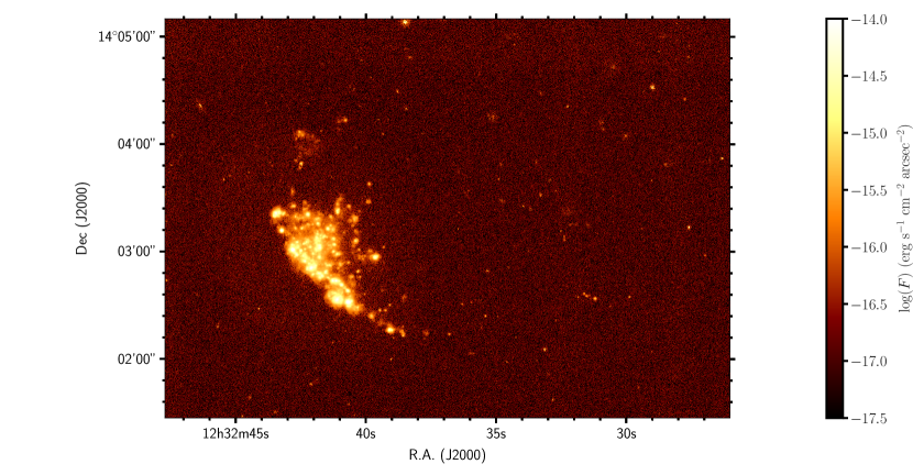
Figure 1: Continuum-subtracted H$\alpha$ image of IC 3476 derived from VESTIGE. With the assumed distance of 16.5 Mpc, 1″= 80 pc.

2.2 FUV ASTROSAT/UVIT imaging

IC 3476 has been observed with ASTROSAT/UVIT (Agrawal 2006; Tandon et al. 2020) in May 2020 using the far-UV filter BaF2 ($\lambda_{c}$ = 1541 Å; $\Delta\lambda$ = 380 Å) during a run dedicated to the observation of a representative sample of Virgo cluster galaxies (proposal A08-003: A FUV Survey of Virgo Cluster Galaxies, PI: J. Hutchings). The observations have been carried out with an integration of 12453 s, reaching a typical surface brightness of $\mu(FUV)$ $\simeq$ 26.8 AB mag arcsec^-2. The field of view of the instrument has a diameter of $\simeq$ 28′and an angular resolution of $\simeq$ 1.5″. The data have been reduced following the prescriptions given in Tandon et al. (2020) using a zero point of $z_{p}$ = 17.771 mag and the astrometry has been checked against the accurate NGVS data (Ferrarese et al. 2012, see below).

2.3 MUSE spectroscopy

The MUSE data were gathered as part of the 095.D-0172 program that studied the host galaxies of core-collapse supernovae (Kuncarayakti et al.2018). Observations were carried out in May 2015 in the Wide Field Mode under excellent seeing conditions ($FWHM$ = 0.74″). The data cover the spectral range 4800-9300 Å and have a spectral resolution $R$ $\sim$ 2600 (1.25 Å sampling per pixel), corresponding to a limiting velocity dispersion $\sigma$ $\sim$ 50 km s^-1 at H$\alpha$ (see Appendix A). The total integration time was 1800 s, with a second exposure of 200 s taken at 2 arcmin from the galaxy to secure the determination of the sky emission. With this integration time, the typical sensitivity of MUSE to low surface brightness emission at H$\alpha$ is $\Sigma(H\alpha)$ $\simeq$ 4 $\times$10^-18 erg s^-1 cm^-2 arcsec^-2. The MUSE data were reduced using ad-hoc procedures developed within the team as extensively described in Fossati et al. (2016), Consolandi et al. (2017), and Boselli et al. (2018b). The astrometry of the MUSE datacube has been finally recalibrated on the VESTIGE data using point sources in the field. A comparison of the flux of the H$\alpha$+[NII] emission line extracted from MUSE with the one obtained from the NB VESTIGE data gives consistent results within 0.3%.

2.4 Fabry-Perot spectroscopy

Fabry-Perot 3D spectroscopic observations of the galaxy IC 3476 were gathered using the GHASP instrument on the 1.93 m Observatoire de Haute Provence (OHP) telescope in May 2017 during the complete Fabry-Perot survey of the Herschel Reference Survey (Gómez-López et al. 2019). The GHASP focal reducer has a Fabry-Perot with a field of view of 5.8 $\times$ 5.8 arcmin² coupled with a 512 $\times$ 512 Imaging Photon Counting System (IPCS) with a pixel scale of 0.68 $\times$ 0.68 arcsec² (Gach et al. 2002). IC 3476 has been observed in dark time and photometric conditions with a total exposure of 4800 s and a typical seeing of 2.0″. The 378 km s^-1 free spectral range of the Fabry-Perot was scanned through 32 channels providing a spectral resolution at H$\alpha$ of $R$ $\simeq$ 10000. The galaxy was observed through an interference filter of 15 Å using the NeI emission line at 6598.95 Å for wavelength calibrations. The data have been reduced as described in Epinat et al. (2008) and Gómez-López et al. (2019). To provide the best combination of angular resolution and signal-to-noise at each position, we applied an adaptive binning technique based on a 2D Voronoi tassellation on the H$\alpha$ data cube producing radial velocity and velocity dispersion maps. This has been done aiming at a fixed $S/N$ = 7.

2.5 Multifrequency data

A large set of multifrequency data useful for the following analysis is available for IC 3476. UV data in the far-UV ($\lambda_{c}$ = 1539 Å; integration time = 107 s) and near-UV ($\lambda_{c}$ = 2316 Å; integration time = 1720 s) bands were obtained with GALEX during the GUViCS survey of the cluster (Boselli et al. 2011). Deep optical images in the $u$, $g$, $i$, and $z$-bands are available from the NGVS survey of the Virgo cluster (Ferrarese et al. 2012). The sensitivity of this survey is $g$ $\simeq$ 25.9 AB mag for point sources (10 $\sigma$) and $\mu(g)$ 29 AB mag arcsec^-2 for extended sources (2$\sigma$), respectively.

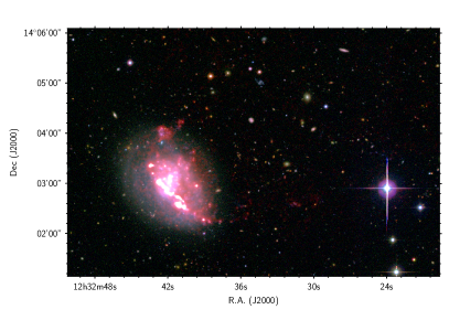
Figure 2: Left: Pseudo-colour image of IC 3476 obtained combining the NGVS (Ferrarese et al. 2012) optical $u$ and $g$ in the blue channel, the $r$ and NB in the green, and the $i$ and the continuum-subtracted H$\alpha$ in the red. Right: same figure produced using a H$\alpha$ continuum-subtracted frame smoothed to an angular resolution of 2.8″to highlight low surface brightness features. The diffuse ionised gas is shown by the coherent emission seen in the red channel on the western side of the galaxy, while the granularity in the eastern side is noise.

Far-IR data include Herschel SPIRE (Ciesla et al. 2012) and PACS (Cortese et al. 2014) at 100, 160, 250, 350, and 500 $\mu$m gathered during the Herschel Reference Survey (HRS, Boselli et al. 2010) and the Herschel Virgo Cluster Survey (HeViCS, Davies et al. 2010), and Spitzer data in the IRAC and MIPS bands from the programs: The Spitzer IRAC Star Formation Reference Survey (P.I. G. Fazio), The Spitzer Survey of Stellar Structures in Galaxies (S4G, Sheth et al. 2010), and VIRGOFIR: a far-IR shallow survey of the Virgo cluster (P.I. D. Fadda). HI data from single dish observations gathered with the Arecibo radio telescope are also available (see Table 1).

3 Analysis

3.1 Broad-band imaging

The colour image of IC 3476 constructed using a combination of NGVS and VESTIGE data (Fig. 2) shows a star forming galaxy with an asymmetric morphology, with prominent blue compact regions located along a banana-shaped structure crossing the old stellar disc at its south-eastern extension from the south-west to the north-east. Similar blue regions, showing the dominance of a young stellar population, are also present at the edge of this elongated structure. The exquisite quality of the CFHT data also shows a dust filament almost parallel to the elongated structure of young stars, suggesting that the south-eastern edge of the galaxy is the one closer to the observer. The dominance of a young stellar population is also visible in the new ASTROSAT/UVIT FUV image (Fig. 3), which shows a clumpy and elongated structure extending up to the outer edges of the stellar disc. The deep NGVS images do not show any low surface brightness extended and diffuse feature outside the stellar disc down to a surface brightness limit of $\mu(g)$ $\simeq$ 29 mag arcsec^-2, ruling out any possible ongoing tidal interaction.

Figure 3: The FUV image of IC 3476 taken with ASTROSAT/UVIT in the BaF2 filter ($\lambda_{c}$ = 1541 Å; $\Delta\lambda$ = 380 Å). Contours show the VESTIGE H$\alpha$ emission at a surface brightness level of $\Sigma(H\alpha)$ = 3 $\times$ 10^-17 erg s^-1 cm^-2 arcsec^-2.

3.2 Narrow-band imaging

The continuum-subtracted H$\alpha$ image is sensitive to the distribution of HII regions made by newly formed ($\lesssim$ 10 Myr) and massive ($M_{\mathrm{star}}$ $\geq$ 10 M_⊙) stars (Kennicutt 1998, Boselli et al. 2009). In IC 3476 the most luminous HII regions are located along the same banana-shaped structure in the south-eastern part of the disc, crossing it from the south-west to the north-east up to its edges (Fig. 1). Other HII regions of lower luminosity are also present on the western side of the galaxy up to the edge of the stellar disc, while they are totally lacking in the eastern direction. This galaxy is also characterised by the presence of several HII regions located outside the stellar disc at the two edges of the elongated banana-shaped structure, at the north and at the south-west of the galaxy. In the south-west they seem to follow a chain starting from the edge of the banana-shaped structure and extending up to $\sim$ 12 kpc in projected distance from the galaxy nucleus ($\sim$ 8 kpc from the edge of the stellar disc), where a complex of several HII regions is present. A few other regions are possibly detected at $\sim$ 17 kpc, as depicted in Fig. 4. All these regions are also present in the ASTROSAT/UVIT FUV image (Fig. 3).

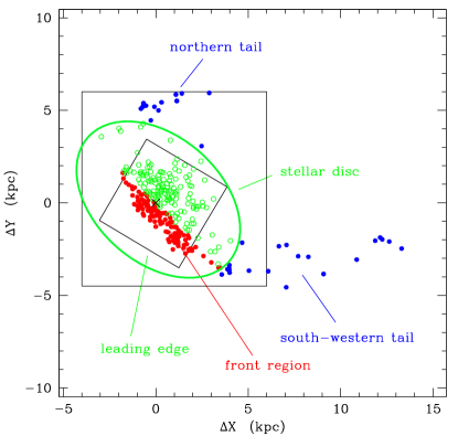
Figure 4: Distribution of the HII regions of IC 3476 with luminosity $L(H\alpha)$ $\geq$ 10³⁶ erg s^-1 and $S/N$ $>$5. Red filled circles are for HII regions in the front structure (101 objects), green empty circles for the other HII regions within the stellar disc (142), and blue filled symbols for HII regions located outside the stellar disc of the galaxy (35), whose extension is measured within the $r$-band isophotal radius at 24 mag arcsec^-2 (from Cortese et al. 2012, see Table 1). The black cross shows the position of the photometric nucleus. The large black box shows the region of the Fabry-Perot datacube analysed in this work, while the small black box the field-of view of MUSE IFU spectrograph, respectively.

3.3 Spectroscopy

3.3.1 Gas kinematics

Figure 5: Velocity map (left) and associated error (right) of the ionised gas derived from MUSE for emission lines with a $S/N$ $>$ 5. The velocity of the gas is given relative to the systemic velocity of the galaxy of -170 km s^-1 derived from HI observations. The white cross, star, and filled circle show the position of the photometric, stellar and gas kinematical centres.

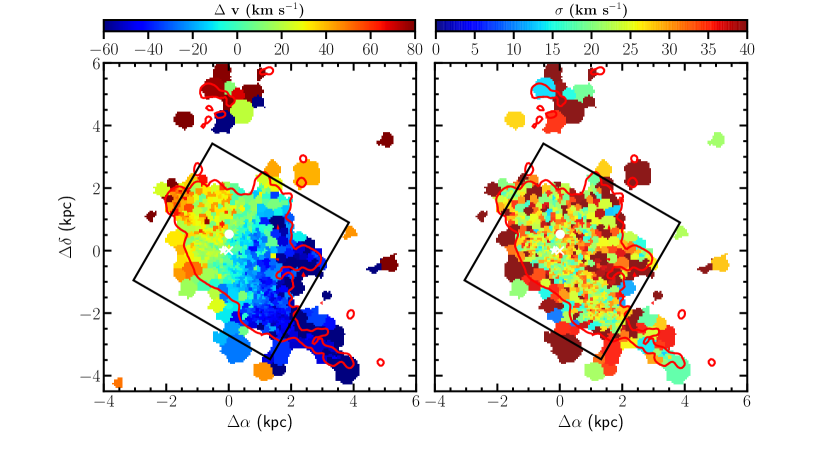
Figure 6: Velocity (left) and dispersion (right) maps of the ionised gas derived from the Fabry-Perot data. The black box indicates the region covered by the MUSE exposure. Red contours show the VESTIGE H$\alpha$ surface brightness at 3 $\times$ 10^-17 erg s^-1 cm^-2 arcsec^-2. The white cross, star, and filled circle show the position of the photometric, stellar and gas kinematical centres, respectively. As for the previous figures, the velocity of the gas is given relative to the systemic velocity of the galaxy of -170 km s^-1.

The 2D velocity field and the velocity dispersion maps of the galaxy derived for the gaseous component using the MUSE and Fabry-Perot data are shown in Fig. 5, and 6, respectively. In order to determine the ionised gas kinematical centre, we have adjusted a rotating disc model to the MUSE data as in Epinat et al. (2008). This model has a fixed centre, systemic velocity, position angle and inclination over the disc and it is built using a Courteau (1997) rotation curve (with $\beta=0$). The method used in this work has been improved with respect to the one of Epinat et al. (2008) so that uncertainties on velocity, flux distribution, and spatial resolution are taken into account. The kinematic centre, the position angle of the major axis, and the inclination of the disc model are left free to vary within a box of $24\times 24$ square arcseconds centred on the coordinates of the morphological centre, between 20° and 60°  and between 50° and 70°, respectively. Two $\chi^{2}$ minimisations were used: the Levenberg-Marquardt algorithm and the multinest bayesian approach (Feroz et al. 2009). While the first method can converge to local minima close the initial guesses, the second one is more robust in finding the absolute minimum. Both approaches led to similar results. The model identified the kinematic centre of the gas at 6.6 arcseconds from the morphological centre (corresponding to $\sim$ 500 pc), as depicted in Fig. 5, with a position angle $P.A.$=54°, an inclination of $i$=52°, and a systemic velocity of $V_{\mathrm{s}}(gas)$=-159 km s^-1. Despite the ionised gas kinematics looking distorted, the axisymmetric model fits fairly well the velocity field with no strong residuals.

The mean kinematical properties of the ionised gas can also be compared to those of the HI gas as derived from the integrated spectrum given in Haynes et al. (2011). The width of the HI line measured at 50% of the peak ($WHI_{\mathrm{50}}$ = 118 km s^-1) is comparable to the dynamic range observed in Fig. 5. The HI spectrum is not a two horns profile as expected for a galaxy of similar mass and inclination, but it is highly asymmetric, suggesting a lack of HI gas in the North-Eastern part of the disc (the galaxy has an HI-deficiency of $HI-def$ = 0.67, Boselli et al. 2014b). As noted by Haynes et al. (2011), however, the HI profile could be partly affected by the Galactic emission.

3.3.2 Stellar kinematics

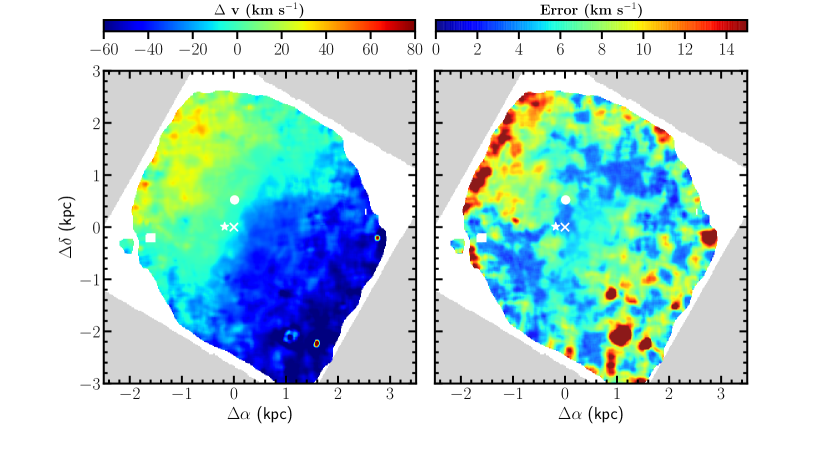
Figure 7: Velocity map (left) and associated error (right) of the stellar disc derived from MUSE for absorption lines with a $S/N$ $>$ 15. The velocity of the stars is given relative to the systemic velocity of the galaxy of -170 km s^-1 derived from HI observations. The white cross, star, and filled circle show the position of the photometric, stellar and gas kinematical centres, respectively.

As for the ionised gas, we derived the stellar kinematical centre by fitting the same model to the stellar velocity field using the same constraints. The stellar kinematical centre is located at 2.2 arcseconds ($\sim$ 180 pc) from the morphological centre, as shown in Fig. 7, and has a position angle of $P.A.$=47°, an inclination of $i$=62°, and a systemic velocity of $V_{\mathrm{s}}(stars)$=-176 km s^-1. Both the position angles and inclinations of the gas and the stars are in quite good agreement, while their centres are separated by $\sim$ 600 pc. Whereas a different centre could induce a different systemic velocity, it seems clear that the observed difference in systemic velocity of the gas and the stars is not due to the different centres since an offset in velocity is observed in any place.

3.3.3 Emission line properties

The excellent quality of the MUSE data allows us to derive several important physical parameters of the ionised gas component of IC 3476. First of all, they can be used to derive the dust attenuation within the gas using the Balmer decrement (Fig. 8). The MUSE data indicate that the typical Balmer decrement of IC 3476 is H$\alpha$/H$\beta$ = 3.72$\pm$0.26 as measured in different regions over the disc of the galaxy, corresponding to $A(H\alpha)$ = 0.68 mag adopting a Cardelli et al. (1989) extinction law, a value comparable to the one observed in galaxies of similar morphological type and stellar mass (Boselli et al. 2009, 2013). It also shows that the highest dust attenuation is observed along the dust features located in the central region and in the NW disc visible in the optical image (Fig. 2), as expected for an efficient screen located in between the emitting regions and the observer. It is interesting to note that the mean dust attenuation in the front region, where most of the bright HII regions are located, is $A(H\alpha)$ = 0.57 mag, and is thus lower than the mean attenuation of the galaxy. Part of the dust generally found in the most active star forming regions might have been displaced in the north-west direction during the interaction.

Figure 8: Distribution of the Balmer decrement derived using the H$\beta$ and H$\alpha$ lines with a $S/N$ $>$5. The black cross, star, and filled circle show the position of the photometric, stellar and gas kinematical centres, respectively. The black rectangle indicates the front region of the galaxy (see Fig. 4).

The [SII]$\lambda$6716/6731 Å line ratio can be used to derive the 2D-distribution of the gas density. The typical value observed in IC 3476 is [SII]$\lambda$6716/6731 $\simeq$ 1.4-1.5 all over the disc of the galaxy, which indicates that the electron density is $n_{\mathrm{e}}$ $\lesssim$ 30 cm^-3 (Osterbrock & Ferland 2006, Proxauf et al. 2014). This upper limit is consistent with the value derived from the H$\alpha$ emission of individual HII regions (see Sect. 3.5).

We also measure the metallicity of the gas using the calibration of Curti et al. (2017) based on the [OIII], H$\beta$, [NII], and H$\alpha$ lines and we obtain typical metallicities ranging from 12+log O/H $\simeq$ 8.70 in the inner disc down to 12+log O/H $\simeq$ 8.50 in the outer regions, consistent with the mean value derived by Hughes et al. (2013) using integrated spectroscopy (12+log O/H = 8.60$\pm$0.12, see Fig. 9). Figure 9 also shows that the highest metallicity is found close to the gas kinematical centre of the galaxy rather than at its morphological centre, consistently with the idea that all the different components of the ISM (gas, dust, metals) have been displaced during the interaction of the galaxy with the surrounding environment.

Figure 9: Distribution of the metallicity derived using the calibration of Curti et al. (2017) using the H$\beta$, [OIII], [NII], and H$\alpha$ lines with a $S/N$ $>$5. The black cross, star, and filled circle show the position of the photometric, stellar and gas kinematical centres, respectively.

The same set of spectroscopic data can be used to derive diagnostic diagrams such as the one proposed by Baldwin et al. (1981, BPT) useful to identify the dominant ionising source of the gas over the disc of the galaxy. Figure 10 shows the BPT diagrams done using the main emission lines detected in the spectrum (H$\beta$, [OIII]$\lambda$5007, [NII]$\lambda$6583, H$\alpha$, and [SII]$\lambda$6716,6731, with a $S/N$ $>$ 5). Despite the strong emission of the galaxy and the sensitivity of MUSE, the detection of the [OI]$\lambda$6300 line is hampered by the contamination of a prominent atmospheric emission line. Figure 10 shows that the gas is photo-ionised by young stars all over the disc, including in the nucleus (both photometric and kinematical) where we do not see the presence of any hard ionising source (AGN). The [OIII]$\lambda$5007/H$\beta$ vs. [SII]$\lambda$6716,6731/H$\alpha$ BPT diagram (lower panels in Fig. 10) indicates that the contribution of stellar photoionisation is dominant on the peaks of the H$\alpha$ emission, where the HII regions are located, while decreases in the diffuse gas, where the contribution of shocks becomes more important.

Figure 10: Left: [OIII]/H$\beta$ vs. [NII]/H$\alpha$ (top), and [OIII]/H$\beta$ vs. [SII]/H$\alpha$ (bottom) BPT diagrams for emission lines with a $S/N$ $>$ 5. The dashed curves separate AGN from HII regions (Kauffmann et al. 2003; Kewley et al. 2001; Kewley et al. 2006). Data are colour coded according to their minimum distance from these curves. The black and grey crosses indicate the typical error on the data for lines with S/N $\simeq$ 15 and S/N $\simeq$ 5, respectively. The grey contours show the distribution of a random sample of nuclear spectra of SDSS galaxies in the redshift range 0.01 - 0.1 and stellar masses 10⁹ $\leq$ $M_{\mathrm{star}}$ $\leq$ 10¹¹ M_⊙. The thick solid lines in the upper left panel show three different photo-ionisation models at different metallicities (0.2, 0.4, 1 Z_⊙; Kewley et al. 2001). Right: Map of the spaxel distribution colour-coded according to their position in the BPT diagram. The cross, star, and filled circle show the position of the photometric, stellar and gas kinematical centres, respectively. The black rectangle indicates the front region of the galaxy (see Fig. 4).

3.4 SED fitting

IC 3476 presents physical properties similar to those observed in other ram pressure stripped galaxies, i.e. a reduced star formation activity in the outer disc with starburst signatures in the inner regions. These properties can be used to quantitatively measure the typical timescales of the quenching phenomenon and of the starburst activity, important parameters for the comparison of the observations with simulations. For this purpose we used the same methodology applied to NGC 4424 (Boselli et al. 2018b). We defined two representative regions within the disc of the galaxy, one located on the leading edge in the eastern part of the disc dominated by old stellar populations where star formation is totally lacking (quenched region), and one in the inner region where most of the brightest HII regions are located (starburst region on the front structure). We then extracted fluxes in 13 different photometric bands (ASTROSAT $FUV$, GALEX $NUV,u,g,r,i,z$, IRAC 3.6, 4.5, 5.7, 8.0 $\mu$m, MIPS 24$\mu$m, and PACS 100 $\mu$m) and in two pseudo-filters (H$\alpha$ in emission and H$\beta$ in absorption, as described in Boselli et al. 2016b) using the flux extraction procedure presented in Fossati et al. (2018). The two regions where fluxes are extracted have a typical size of $\sim$ 400 arcsec² and are thus fully resolved in all these photometric bands. The two selected regions are located within the MUSE field, we thus used the MUSE data to measure the H$\alpha$ flux in emission uncontaminated by the [NII] lines and corrected for dust attenuation using the mean Balmer decrement within each region ($A(H\alpha)$ = 0.0 mag in the quenched region, $A(H\alpha)$ = 0.57 in the starburst region) and the age-sensitive H$\beta$ absorption line (Poggianti & Barbaro 1997). The H$\beta$ absorption line in the pseudo-filter is measured using the observed light-weight mean spectrum in the quenched region, while the one corrected for the line emission using the GANDALF code in the starburst region. We then fit the observed spectral energy distributions (SED) of these two regions using the CIGALE fitting code (Noll et al. 2009, Boquien et al. 2019) coupled with the Bruzual & Charlot (2003) stellar population models derived with a Chabrier IMF for the stellar continuum and the Draine & Li (2007) models for the dust emission, assuming a Calzetti attenuation law with 0 $\leq$ $E(B-V)$ $\leq$ 0.8 and a solar metallicity. To quantify the time elapsed since the beginning of the starburst phenomenon in the inner regions or that of the truncation of the star formation activity in the outer disc we use a parametrised abruptly truncated star formation law characterised by the following free parameters: the rotational velocity of the galaxy (which mainly describes the secular evolution of an unperturbed rotating disc, see Boselli et al. 2016b), the quenching age $QA$ (time elapsed since the beginning of the quenching of the star formation activity or of the starburst phase), and the quenching factor $QF$ ($QF$ = 0 for unperturbed SFR, $QF$ = 1 for totally quenched SFR, $QF$ = -1 for a SFR increased by a factor of 100%).

Figure 11: Far-UV to far-IR SED of the two selected regions within IC 3476. In each panel the observational data and their error bars are indicated with red filled dots, upper limits with blue triangles. The solid black line shows the best fit model derived with CIGALE. The inset shows the colour image of the galaxy with overlayed in red the region analysed.

Figure 12: Best model fit of the stellar continuum obtained with CIGALE (black) is compared to the MUSE spectrum (red) in the H$\beta$ line after the emission is removed using GANDALF for the starburst (left) and quenched (right) regions. The best model has been scaled on the Y-axis to match the observed spectrum.

The results of the fit are shown in Fig. 11 and Fig. 12. The quality of the fit is excellent in both regions and indicates that both the quenching and the starburst episodes are very recent ($QA$ = 32 $\pm$ 12 Myr for the quenched region, $QA$ = 16 $\pm$ 50 Myr for the starburst region). The quenching episode totally stopped the star formation activity in the outer disc at the front edge of the galaxy ($QF$ = 1) while the star formation activity increased by $\sim$ 161 % in the inner regions. Similar $QF$ and slightly longer timescales ($QA$ = 103 $\pm$ 30 Myr for the quenched region, $QA$ = 40 $\pm$ 92 Myr for the starburst region) are obtained using the smooth quenching episode described in Boselli et al. (2016b). We further checked the robustness of these results by applying the SED fitting procedure described in Fossati et al. (2018) based on a Monte Carlo Spectro-Photometric technique, which combines both the broad-band photometric points and the whole spectrum obtained with MUSE in the fit. Using a similar parametrisation for the description of the secular evolution of the star formation history of the galaxy, and applying an exponentially declining star formation model to describe the quenching episode, the fit gives $Q_{Age}$ = 55 $\pm$ 10 Myr for the time elapsed since the beginning of the perturbation and $\tau_{Q}$ = 5 $\pm$ 1 Myr for the typical timescale for the decrease of the activity, two values very close to those obtained with CIGALE for an abrupt truncation. We can thus confidently claim that the leading edge of the galaxy rapidly quenched its star formation activity $\lesssim$ 100 Myr ago. This quenching episode was followed by a starburst activity in the inner regions.

3.5 Properties of the HII regions

We use the HIIphot data reduction pipeline (Thilker et al. 2000) to derive the physical properties of individual HII regions inside the disc of the perturbed galaxy and in the tails of stripped material. This code, which uses a recognition technique based on an iterative growing procedure to identify single HII regions over the emission of a varying stellar continuum, is optimised to extract the properties of these compact structures from NB imaging data. We refer the reader to Thilker et al. (2000), Scoville et al. (2001), Helmboldt et al. (2005), Azimlu et al. (2011), Lee et al. (2011), and Liu et al. (2013) for an accurate description and for the utilisation of this code for this purpose. As described in Boselli et al. (2020), we run this code jointly on the H$\alpha$ continuum-subtracted, the H$\alpha$ NB, and the stellar continuum image, the last derived as explained in Sect. 2.1.

Thanks to the excellent quality of the VESTIGE data in terms of sensitivity and angular resolution, the HIIphot code detects HII regions down to luminosities $L(H\alpha)$ $\simeq$ 10³⁶ erg s^-1 and equivalent radii $r_{eq}(H\alpha)$ $\simeq$ 40 pc, defined as in Helmboldt et al. (2005), i.e. the radii of the circles of surface equivalent to the area of the detected HII region down to a surface brightness limit of $\Sigma(H\alpha)$ = 3 $\times$ 10^-17 erg s^-1 cm^-2 arcsec^-2. Equivalent radii and diameters are corrected for the effects of the point-spread function (PSF) following Helmboldt et al. (2005). At these low emission levels where crowdness becomes important the code might suffer for incompleteness (e.g. Pleuss et al. 2000; Bradley et al. 2006). We thus limit the present analysis to a comparative analysis of the physical properties of HII regions located inside and outside the stellar disc, in the stripped material, and detected with a signal-to-noise $S/N$ $>$ 5, avoiding any statistical analysis which would require a complete sample. We expect that this comparative analysis, which is based on data extracted from the same images, does not suffer from strong systematic biases. We recall, however, that the most crowded regions are probably more frequent within the disc of IC 3476, where also the stellar continuum might be dominant, while totally lacking in the stripped tail. We also notice that the two BPT diagrams show a few HII regions with Seyfert-like spectra (see Fig. 10). These, however, are only $<$ 0.2 % and $<$ 0.5 % of the spaxels, their contamination in the analysis presented in the next sections is thus negligible.

Figure 13: Properties of the HII regions of IC 3476 with luminosity $L(H\alpha)$ $\geq$ 10³⁶ erg s^-1 and $S/N$ $>$5. Upper left: H$\alpha$ luminosity function. Upper right: relationship between the H$\alpha$ luminosity and the equivalent diameter. Lower left: distribution of the equivalent diameter. Lower right: distribution of the electron density. Black histograms are for all HII regions, red and blue filled histograms and symbols are for HII regions located on the front region within the disc and for HII regions in the tails outside the disc, respectively; green hased histograms and empty symbols for HII regions within the stellar disc but outside the front structure. All H$\alpha$ luminosities are corrected for [NII] contamination using the mean [NII]/H$\alpha$ ratio derived within the MUSE field, [NII]/H$\alpha$ = 0.29. Electron densities are also corrected for Balmer decrement ($A(H\alpha)$ = 0.68 mag) for comparison with other works. The dotted line in the upper right panel shows the $n_{\mathrm{e}}$ = 1 cm^-3 relation. Equivalent diameters and electron densities are plotted only for those regions where the correction for the effect of the PSF is less than 50%.

3.5.1 Physical properties

We first identify the galaxy HII regions as those located within the $r$-band isophotal radius measured at 24.0 mag arcsec^-2 by Cortese et al. (2012; $r_{\mathrm{ISO}}(r)$ = 64.5″), and assuming $e$ = 0.29, and $P.A.$ = 45 deg. (from North, counterclockwise, where $e$ and $P.A.$ are the ellipticity and the position angle of the corresponding elliptical profile). Those oustide the stellar disc are mainly located along the tails of stripped gas present in the continuum-subtracted H$\alpha$ image (Fig. 1). HIIphot detects 278 HII regions with $L(H\alpha)$ $\geq$ 10³⁶ erg s^-1 and $S/N$ $>$5 associated to the galaxy, and 35 outside the stellar disc, as depicted in Fig. 4 (blue filled symbols). The HII regions located within the stellar disc (green ellipse in Fig. 4) can be further divided into those in the front region (red filled symbols, located at the west of a line crossing the galaxy at 0.67″south from its nucleus with a $P.A.$ = 45 deg. measured counterclockwise from the North, 101 objects) and those in the back of the disc (green empty symbols, 142 objects). For these HII regions we derive the H$\alpha$ luminosity function (where for comparison with other works $L(H\alpha)$ is corrected only for Galactic extinction and [NII] contamination assuming the mean value derived from the MUSE data, [NII]/H$\alpha$ = 0.29), the $L(H\alpha)$ vs. size relation (where $D_{\mathrm{eq}}$ is the equivalent diameter), the size distribution and the mean electron density $n_{\mathrm{e}}$ distribution (Fig. 13). The mean electron density $n_{\mathrm{e}}$ is derived following Scoville et al. (2001) with the relation (case B recombination, from Osterbrock & Ferland 2006):

$$n_{\mathrm{e}}=43\bigg{[}\frac{(L_{cor}(H\alpha)/10^{37}\leavevmode\nobreak\ \rm{erg\leavevmode\nobreak\ s^{-1}})(T/10^{4}\leavevmode\nobreak\ \rm{K})^{0.91}}{(D_{eq}/10\leavevmode\nobreak\ \rm{pc})^{3}}\bigg{]}^{1/2}\leavevmode\nobreak\ \leavevmode\nobreak\ [\rm{cm^{-3}}]$$ (1)

where $L_{cor}(H\alpha)$ is the H$\alpha$ luminosity of the individual HII regions corrected for [NII] contamination (see above) and dust attenuation assuming the mean value derived from the MUSE IFU data ($A(H\alpha)$ = 0.68 mag), and $T$ the gas temperature (here assumed to be $T$ = 10000 K). Equivalent diameters and electron densities are plotted only for those regions where the correction for the effect of the PSF is less than 50%. We notice that the typical values of the electron densities derived using Eq. 1 ($n_{\mathrm{e}}$ $\lesssim$ 8 cm^-3) are consistent with the upper limit derived using the [SII] doublet ratio using the MUSE data ($n_{\mathrm{e}}$ $\lesssim$ 30 cm^-3).

The analysis of Figures 4 and 13 indicates that:

1) The most luminous HII regions ($L(H\alpha)$ $\geq$ 10³⁸ erg s^-1) are present only within the disc of the galaxy and most of them are located along the front region crossing the disc, suggesting that they have been probably formed during the interaction of the galaxy ISM with the surrounding intracluster medium (ICM) through ram pressure.

2) The HII regions located along the tails of stripped material have typical luminosities $L(H\alpha)$ $\lesssim$ 10³⁷ erg s^-1, most of them sizes $D_{\mathrm{eq}}$ $\lesssim$ 100 pc, and electron densities $n_{\mathrm{e}}$ $\lesssim$ 3 cm^-3, corresponding to the faint end distribution of the values found in the HII regions located within the stellar disc of the galaxy. We caution, however, that the parameters derived for the HII regions with the lowest luminosities per unit size might be biased since HIIphot is optimised to identify and measure the emission of HII regions located over a strong stellar continuum emission, which is mainly lacking in the tails of stripped material.

3) The HII regions located on the front of the galaxy, on the contrary, are on average more luminous per unit size than those located on the back of the disc. This effect is mainly evident in the most luminous ($L(H\alpha)$ $\geq$ 10^37.5 erg s^-1) and extended ($D_{\mathrm{eq}}$ $\geq$ 250 pc) HII regions, where $L(H\alpha)$ is a factor of $\simeq$ 2.5 higher than measured in objects of similar size elsewhere in the disc. This results in a systematic difference in the mean electron density of the HII regions in the front ($n_{\mathrm{e}}$ = 3.1 $\pm$ 1.3 cm^-3), in the back of the galaxy ($n_{\mathrm{e}}$ = 1.9 $\pm$ 0.9 cm^-3), and in the tail ($n_{\mathrm{e}}$ = 1.6 $\pm$ 1.0 cm^-3, where $\pm$ gives 1-$\sigma$ of the distribution). A Kolmogorov-Smirnov test indicates that the probability that the three distributions are drawn from the same parent population is $P$ = 1.9% ($n_{\mathrm{e}}(tail)$ vs. $n_{\mathrm{e}}(front\leavevmode\nobreak\ region)$), $P$ = 5.2% ($n_{\mathrm{e}}(disc)$ vs. $n_{\mathrm{e}}(front\leavevmode\nobreak\ region)$), and $P$ = 4.6% ($n_{\mathrm{e}}(disc)$ vs. $n_{\mathrm{e}}(tail)$). Comparable differences are obtained if more stringent criteria on the PSF correction are adopted. It must be noticed that an increase of the electron density might artificially result from an underestimate of the size of the HII regions in the crowded regions. This effect, however, should be negligible because the distribution in size within the crowded, front HII regions is not biased vs. small objects compared to that of the other HII regions in the disc probably because of the adopted high surface brightness level for the identification of the equivalent isophotal diameters. This is also evident for the HII regions in the tail, which have the smallest sizes despite their very low aggregation. This result is also robust vs. the adopted correction for [NII] contamination and dust attenuation since similar differences are seen when the VESTIGE NB imaging data are corrected using a 2D map derived from the fully resolved MUSE data where these are available (thus only on the stellar disc of the galaxy).

The MUSE data also indicate that the mean [OIII]$\lambda$5007/H$\beta$ measured within the front HII regions ([OIII]$\lambda$5007/H$\beta$ = 0.77$\pm$0.35) is slightly higher than that measured on the other HII regions in the disc ([OIII]$\lambda$5007/H$\beta$ = 0.64$\pm$0.56) (Fig. 14). Since the ionisation energy of [OIII] is 54.9 eV, this suggests that in the front HII regions the radiation is harder and the ionising stars are possibly slightly younger than in the other regions (Citro et al. 2017), although part of this difference could also be due to a difference in the mean metallicity of the two regions. A younger age of these HII regions is also suggested by their smaller size per unit luminosity than the other disc HII regions (e.g. Ambrocio-Cruz et al. 2016, Boselli et al. 2018c).

Figure 14: [OIII]/H$\beta$ vs. [NII]/H$\alpha$ (left), and [OIII]/H$\beta$ vs. [SII]/H$\alpha$ (right) BPT diagrams for the HII regions located in the front region (red filled dots) and within the galaxy disc (green empty circles) as depicted in Fig. 4. The dashed curves separate AGN from HII regions (Kauffmann et al. 2003; Kewley et al. 2001; Kewley et al. 2006).

The typical age of the star forming complexes in the tail of the galaxy can be measured using their H$\alpha$ and FUV emission extracted within given apertures as done in the tail of NGC 4254 by Boselli et al. (2018c). We refer the reader to that work for a detailed description of the methodology. For this purpose, we chose apertures optimised to match the angular resolution of the UVIT image ($>$ 1.5″diameter) and extracted fluxes within the FUV and continuum-subtracted H$\alpha$ images using the same procedure described in Sect. 3.4. We then corrected H$\alpha$ for [NII] contamination assuming the mean value measured within the galaxy disc ([NII]/H$\alpha$ = 0.29) and converted it into Lyman continuum fluxes using the relation (Boselli et al. 2016b):

$${LyC\leavevmode\nobreak\ \mathrm{[mJy]}=\frac{1.07\times 10^{-37}\leavevmode\nobreak\ [L(H\alpha)/\mathrm{erg\,s}^{-1}]}{[D/\mathrm{Mpc}]^{2}}}$$ (2)

and then into a FUV-H$\alpha$ colour index (where $FUV$ is in AB mag):

$${H\alpha-FUV=-2.5\log(LyC)+20-FUV}$$ (3)

We then compared these observed colours to the synthetic colours of HII regions derived assuming a star formation history defined as:

$${\mathrm{SFR}(t)=\epsilon\,t\,\mathrm{e}^{-t/\tau}\leavevmode\nobreak\ \leavevmode\nobreak\ \leavevmode\nobreak\ \leavevmode\nobreak\ \leavevmode\nobreak\ \rm{M_{\odot}yr^{-1}}}$$ (4)

where the e-folding time $\tau$ is set to 3 Myr, consistent with the typical age of giant ($L(H\alpha)$ $\simeq$ 10³⁷ erg s^-1) HII regions in the Milky Way or in other nearby galaxies (Copetti et al. 1985; Tremblin et al. 2014). The synthetic colours of HII regions have been derived using the CIGALE SED fitting code, assuming Bruzual & Charlot (2003) population synthesis models with a Salpeter IMF, and adopting three different mean attenuations ($E(B-V)$ = 0.0, 0.1, 0.2). Attenuations lower than those measured within the stellar disc are expected since these external HII regions have been formed within the metal-poor gas mainly stripped from the outer disc, as indeed observed in the tail of jellyfish galaxies (e.g. Fossati et al. 2016, Poggianti et al. 2019). The comparison between synthetic and observed colours given in Fig. 15 clearly shows that the typical age of the star forming complexes in the tail is $\simeq$ 20 Myr, and reaches 30 Myr only in one region located close to the galaxy. These ages are slightly younger than those measured in the tail of NGC 4254 ($\lesssim$ 100 Myr), where the star forming complexes have been selected in the NUV band. The age of the HII regions in the tails is comparable to that of the inner starburst. It is also fairly comparable to the time necessary for the galaxy to travel $\sim$ 15 kpc on the plane of the sky ($\sim$ 10 Myr), the projected length of the tails, at $\sim$ 1500 km s^-1 = $\sqrt{2}\times\sigma_{Virgo}$, where $\sigma_{Virgo}$ is the typical line of sight velocity dispersion of star forming systems within the Virgo cluster ($\sigma_{Virgo}$ $\sim$ 1000 km s^-1; Boselli et al. 2014a). It is thus conceivable that these external HII regions have been formed at the turbulent edges of the galaxy during its interaction with the surrounding medium and stripped away as collapsing gas in giant molecular clouds.

Figure 15: Left panel: variations of the synthetic $H\alpha$-$FUV$ age-sensitive colour index as a function of time derived for the star formation history given in Eq. 4. Different colours are used for three different dust attenuations: $E(B-V)$ = 0.0 (blue), 0.1 (green), and 0.2 (red). The black solid line shows the median of the observed colour distribution of the star complexes in the tail of IC 3476, the grey lines the 16% and the 84% quartiles of their distribution. Right panel: observed distribution of the $H\alpha$-$FUV$ colour index.

3.5.2 Kinematical properties

We compare the physical properties of the HII regions derived in the previous section to their kinematical properties determined using the spectroscopic data. For this purpose we use the Fabry-Perot data which have the required spectral resolution ($R$ $\simeq$ 10000) to measure velocity dispersions down to $\sim$ 13 km s^-1. As indicated in the Appendix, the spectral resolution of MUSE (R $\simeq$ 2600, corresponding to a limit in the velocity dispersion of $\sigma$ $\sim$ 50 km s^-1), is not sufficient for this purpose. To minimise the possible confusion due to the lower angular resolution of the Fabry-Perot data with respect to the imaging data, we limit this analysis to the regions where the $S/N$ is sufficiently high and the velocity dispersion is uncontaminated ($\leq$ 10%) by the adjacent HII regions or the diffuse background emission as indicated in the Appendix.

Figure 16: Kinematical properties of the HII regions of IC 3476 with luminosity $L(H\alpha)$ $\geq$ 10³⁶ erg s^-1 and $S/N$ $>$5, where the instrumental limit in the velocity dispersion is $\sigma$ $\simeq$ 13 km s^-1. Upper left: H$\alpha$ luminosity vs. velocity dispersion. Upper right: equivalent diameter vs. velocity dispersion. Lower left: electron density vs. velocity dispersion. Lower right: kinematical age vs. equivalent diameter. Red filled symbols are for HII regions located on the front structure, green empty symbols for the other HII regions within the stellar disc, respectively. All H$\alpha$ luminosities are corrected for [NII] contamination and for Balmer decrement using the [NII]/H$\alpha$ and H$\alpha$/H$\beta$ ratios measured using the MUSE data within each individual region. Equivalent diameters and electron densities, defined as described in the text, are plotted only for HII regions where the PSF correction is less than 50%. The black solid line and the dotted lines show the mean relation and the envelope of points derived in the LMC by Ambrocio-Cruz et al. (2016).

Figure 16 shows the relationship between the H$\alpha$ luminosity $L(H\alpha)$, the equivalent diameter $D_{\mathrm{eq}}$, and the electron density $n_{\mathrm{e}}$ with the velocity dispersion $\sigma$ of the ionised gas within resolved HII regions located on the disc of the galaxy and in the starbursting structure. It also shows the relationship between the kinematical age of the individual HII regions, defined as $k_{\mathrm{age}}$ = $D_{\mathrm{eq}}$/$\sigma$, with the equivalent diameter. Since all the points plotted in these panels are included within the MUSE field, where the H$\alpha$ emission is sufficiently high to allow an accurate estimate of the velocity dispersion in the Farby-Perot cube, the H$\alpha$ data are here corrected for [NII] contamination and dust attenuation using their local estimate in the MUSE data. The velocity dispersion of the HII regions ranges between 15 $\lesssim$ $\sigma$ $\lesssim$ 40 km s^-1, and is thus comparable to that observed in the giant HII regions of other nearby galaxies (e.g. Smith & Weedman 1970, Chu & Kennicutt 1994, Ambrocio-Cruz et al. 2016, Bresolin et al. 2020). The first three plots do not show any correlation, but suggest that the HII regions located on the front region formed after the dynamical interaction with the IGM, have, on average, a higher H$\alpha$ luminosity and electron density per unit velocity dispersion than their counterparts on the stellar disc, with a similar distribution of their size. The lower right panel shows that the HII regions formed in the front region and those located elsewhere in the disc share the same kinematical age vs. equivalent diameter relation. Given the relationship between star formation rate, gas column density, and velocity dispersion (e.g. Elmegreen 2015):

$$\Sigma_{\mathrm{SFR}}=\epsilon_{\mathrm{eff}}\left(\frac{4}{\sqrt{3}}\right)G\frac{\Sigma_{\mathrm{gas}}^{2}}{\sigma}$$ (5)

where $\epsilon_{\mathrm{eff}}$, the star formation efficiency per unit free fall time, is a fairly constant parameter in different environments (Federrath & Klessen 2012), it is thus conceivable that the observed increase of star formation activity along the front region is mainly due to an increase of the gas volume density occured after the displacement of the external gas along the stellar disc pushed by the dynamical pressure exerted by the surrounding IGM during the mostly edge-on interaction (Elmegreen & Efremov 1997). The increase of the external pressure favors the formation of molecular gas (Blitz & Rosolowsky 2006) and increases the star formation activity (Bieri et al. 2016).

4 Simulations

4.1 Methodology

To understand the origin of the peculiar features observed in the data we perform idealised hydrodynamical simulations of a galaxy with properties similar to IC 3476 subject to ram-pressure stripping. We stress that the purpose of this exercise is not that of identifying the simulation which best reproduces all the observed properties of IC 3476, which would require to run several low resolution simulations on a large grid of input parameters, but rather to understand, using a high resolution simulation, the nature of the various physical processes acting on the different galaxy components and its effects on the stripped gas. Our setup consists of an isolated galaxy at rest at the centre of a 600 kpc cubic periodic box. The galaxy is made of a $2.5\times 10^{11}\rm\,M_{\odot}$ dark matter halo, a $1.2\times 10^{9}\rm\,M_{\odot}$ stellar disc, and a $2\times 10^{9}\rm\,M_{\odot}$ gaseous disc (see Table 1 for a comparison with IC 3476). We generated the initial conditions using MakeDisk (Springel et al. 2005), which assumes a global equilibrium of the system, and obtained a scale radius of the disc $r_{0}\sim 2.6$ kpc. We notice that this scalelength is a factor of 1.7 larger than the one measured in IC 3476. This might moderately overestimate the effects of stripping. We conservatively assume a scale height $h_{0}=0.1r_{0}$. These parameters lead to a rotational velocity of the galaxy in the range -60 $\lesssim$ $v_{\mathrm{rot}}$ $\lesssim$ 60 km s ^-1 at 2 kpc, -80 $\lesssim$ $v_{\mathrm{rot}}$ $\lesssim$ 80 km s ^-1 at 3 kpc, reaching $\sim$ 100 km s^-1 at $\sim$ 10 kpc. The box is filled with a hot, low-density gas ($n_{\mathrm{e}}$ = 2 $\times$ 10^-4 cm^-3), aimed at representing the IGM, that can be set in relative motion with the galaxy to mimic the system motion throughout the cluster. We note that, although a more accurate description of the IGM would require variable density and velocity of the system relative to the IGM (Tonnesen 2019), for the purpose of the current study we assume for simplicity a constant density/velocity gas.

In order to accurately assess the effect of ram-pressure stripping on the system, we performed two different runs, where the ICM is moving along the $z$-direction at 1200 and 2000 $\rm km\,s^{-1}$, respectively. These two velocities roughly correspond to the observed stellar line of sight velocity with respect to the mean velocity of the cluster (1131 km s^-1), which can be considered as a lower limit, and the same velocity $\times$ $\sqrt{3}$ (1959 km s^-1) which takes into account the velocity of the galaxy on the plane of the sky. The resulting pressure for a velocity of 2000 km s^-1 is $P$ = 1.5 $\times$ 10^-11 dyn cm^-2. We also performed a reference run where we assume the ICM at rest, aimed at representing the evolution of the system in the case of no ram-pressure. To be consistent with the observations, the galaxy is inclined by 70$\degr$ relative to the $z$-axis.

We performed our runs with gizmo (Hopkins 2015), descendant of Gadget 2 (Springel 2005) and Gadget 3 (Springel et al. 2008), employing the sub-grid models for star formation and stellar feedback (supernovae, wind, and stellar radiation) described in Lupi & Bovino (2020) and Lupi et al. (2020). Gas cooling and chemistry are modelled via krome (Grassi et al. 2014), using the metal network described in Bovino et al. (2016) and already employed in several works (Capelo et al. 2018, Lupi & Bovino 2020, Lupi et al. 2020). The mass resolution for the galaxy is set to $2.5\times 10^{5}\rm\,M_{\odot}$ for dark matter, and $2000\rm\,M_{\odot}$ for gas and stars. Although a higher resolution would allow for a better sampling of small star clusters in the tails, our choice is mainly dictated by the fact that a proper sampling of the IMF requires at least  1000 Msun/particle, and by the computational cost of the runs. The spatial resolution is defined by the Plummer-equivalent gravitational softening, that is kept fixed for dark matter and stars at 80 and 10 pc, respectively. For gas, we employ fully adaptive gravitational softening, with the kernel around each cell defined to encompass an effective number of 32 neighbours, and the maximum resolution set at 1 pc. The wind is initially sampled with a 100 times lower resolution, but it is refined on-the-fly in the simulation via particle splitting, when at least 75 per cent of the kernel of the wind cell is covered by higher-resolution gas. This approach allows us to keep a large enough box to avoid boundary effects on the galaxy and at the same time to save computational time evolving the low-density ICM in the regions where no interaction with the galaxy occurs. Because of the initial configuration of the system, where turbulence due to stellar feedback is not present, we expect a star formation burst to occur at the beginning of the simulation. To reduce this numerical effect we let the stellar particles already present in the system to explode as supernovae stochastically, assuming a uniform age distribution with average 3.5 Gyr. In addition, instead of starting all the runs at $t=0$, we start the two ram-pressure simulations taking the results of the reference run at $t=100$ Myr, i.e. at the end of the initial burst. The different gas phases, neutral atomic, molecular, and ionised, are a direct output of the simulations. They results from the consistent non-equilibrium chemical evolution of the gas (Lupi et al. 2018, Capelo et al. 2018). For the following analyses, we select the particles that initially belong to the galaxy, and exclude the gas belonging to the ICM, independently of its thermodynamic/chemical state.

4.2 Results

4.2.1 2D distribution

The results of the simulations are shown in Figures 17 to 22. For a comparison with the observations we plot here the output of the simulations at those epochs which better match the observed data. To ease the comparison with IC 3476, the simulated galaxy is first projected at an inclination of 45°, then rotated on the plane of the sky by 45°. For this projection, this implies that the line-of-sight velocity of the wind is $V_{\mathrm{los}}(wind)$ = $\cos(25\degr)\times v(wind)$, while those on the plane of the sky $V_{\mathrm{X,Y}}(wind)$ = $\sqrt{2}\times\cos(65\degr)\times v(wind)$, which, for a wind of 2000 km s^-1, gives respectively $V_{\mathrm{los}}(wind)$ $\simeq$ 1800 km s^-1 and $V_{\mathrm{X,Y}}(wind)$ $\simeq$ 600 km s^-1. Given that the line-of-sight velocity of IC 3476 with respect to the cluster is 1131 km s^-1, the velocity of the galaxy on the plane of the sky should be $\sim$ 1650 km s^-1, thus the projected extension of the gas and of the stellar tails are underestimated in Fig. 17 and 18. We focus on the simulations done with a wind of 2000 km s^-1 which are more representative of IC 3476. The results obtained with a wind of 1200 km s^-1 are similar, although less pronounced.

Figures 17 and 18 show the 2D distribution of the different gas components (HI, H₂, HII, and total, defined as HI+H₂+HII+He+metals) and of the star formation activity of the simulated galaxy undergoing an external wind of 2000 km s^-1, 150 Myr after the beginning of the interaction. The gas distribution is highly asymmetric, with most of the gas (in all its phases) located on one side of the galaxy and in prominent tails extending up to $\sim$ three times the stellar disc. The leading side of the galaxy is completely deprived of gas. The dominant gas phase in the tail is the ionised one, which has a diffuse distribution as the atomic gas, while the molecular phase is only located in thin filamentary structures. Because of the lack of gas, the star formation activity is totally quenched in the leading side of the stellar disc, while boosted in the front edge of the gas at the interface between the IGM and the ISM ($\Sigma_{\mathrm{SFR}}$ $\simeq$ 0.1-0.5 M_⊙ yr^-1 kpc^-2) where its density is maximal ($\Sigma_{\mathrm{gas}}$ $\simeq$ 20-50 M_⊙ pc^-2). Star formation is also present far from the stellar disc in the condensed regions located along the filamentary structures seen in H₂. Figure 18 also shows that the brightest star forming regions have been formed at the leading edge located at the the South-East of the galaxy, at the boundary region between the hot ICM and the cold ISM (front region), consistently with the observations.

Figure 17: 2D distribution of the total (HI, H₂, HII, He, and metals; upper left panel), ionised (upper right), atomic (lower left), and molecular (lower right) gas components of the simulated galaxy undergoing a wind of 2000 km s^-1, 150 Myr after the beginning of the interaction. The model galaxy is oriented as IC 3476 on the plane of the sky. The cyan cross in the upper left panel shows the stellar centre, the contours the stellar disc, while those in the lower panels the distribution of the star forming regions. The green arrow indicates the direction of the wind.

Figure 18: 2D distribution of the star formation activity of the simulated galaxy undergoing a wind of 2000 km s^-1 150 Myr after the beginning of the interaction. The green arrow indicates the direction of the wind.

4.2.2 Gas deficiency

Figure 19 shows the time variation of the gas deficiency parameter, defined as the logarithmic difference between the total mass of the atomic, molecular, and ionised gas mass of the unperturbed galaxy and that of the simulated perturbed systems measured at the same epoch. All entities are geometrically measured within a circular aperture (projected as an ellipse according to the inclination of the galaxy) with radius 3.4 times the stellar disc scalelength of the simulated galaxy, corresponding roughly to 9 kpc, thus at $\sim$ 2 optical isophotal radii. While the aperture is centered at each time step on the centre of mass of the stellar component of the galaxy, the radius is kept fixed in time since the new stellar mass formed is not large enough to significantly change the disc size over the short timescales of the simulations. Figure 19 can be thus directly compared with the observations. Figure 19 shows that the HI-deficiency parameter monotonically increases with time reaching $HI-def$ $\simeq$ 0.4 at $t$ $\simeq$ 280 Myr for an external wind of 2000 km s^-1, a value slightly lower than the one observed in IC 3476 ($HI-def$ = 0.67; Boselli et al. 2014b). On the contrary, the H₂ and HII-deficiency parameters first abruptly decrease to $\simeq$ -0.2 and -0.4 and later increase to $H_{\mathrm{2}}-def$ $\simeq$ 0.3 after 350 Myr and $HII-def$ $\simeq$ 0.4 after 400 Myr. The variation with time of the HI-deficiency parameter can be easily explained by a continuous gas stripping due to the wind flow. The fact that the simulation does not reach the observed value of $HI-def$ = 0.67 just indicates that the simulated stripping process is not sufficiently efficient, and this can be due to the assumed impact parameters (the inclination of the galaxy disc with respect to the wind flow might be lower than 70$\degr$), by an underestimate of the assumed infall velocity or density profile, or by the limited resolution of the simulations. On the other hand, the model galaxy is more extended that IC 3476, thus stripping should be more efficient in the model. The almost edge-on stripping process pushes on short timescales ($t$ $\lesssim$ 100 Myr) the gas located on the leading side of the galaxy over the stellar disc. The increase of the external pressure facilitates the formation of molecular clouds on the disc which leads to a decrease of the molecular gas deficiency and to an increase of the HI deficiency. On longer timescales ($t$ $\gtrsim$ 200 Myr) the molecular gas condensed in high density regions is transformed into stars while the diffuse component, which is located within the inner disc, is reached by the external pressure and removed along with the HI component. The observed abrupt decrease of the ionised gas deficiency just after the beginning of the interaction could be due to a combined effect of an increase of the star formation activity boosted by the supply of fresh gas on the disc with a change of phase of the gas located on the leading side, shock-ionised during the interaction on the interface between the cold ISM and the hot IGM.

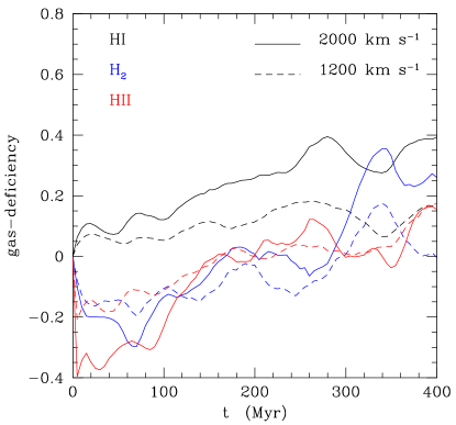
Figure 19: Variation of the gas deficiency parameter in the different phases (black: HI; blue: H₂; red: ionised) as a function of time for the simulated galaxy subject to an external wind of 2000 km s^-1 (solid) and 1200 km s^-1 (dashed).

4.2.3 Gas phases in the tail

Figure 20 shows the time variation of the fraction of the different gas phases-to-total gas measured outside the disc of the simulated galaxy at a radius $r$ $>$ 9 kpc from the nucleus. The interpretation of this figure is complicated because both the numerator (HI, H₂, HII) and the denominators (HI + H₂ + HII) of the stripped gas fraction change with time. At the beginning of the stripping process the gas in the tail is at $\sim$ 40% HI, and 30% H₂ and HII, respectively. The HI fraction increases to $\sim$ 60% after $\sim$ 250 Myr, and slightly decreases afterwards. The molecular gas fraction first drops to $\sim$ 20% after 50 Myr, increases up to $\sim$ 35% at 150 Myr, and slowly decreases to $\sim$ 20% at 400 Myr after the beginning of the interaction. The ionised gas component has an opposite trend, with an increase in the first 50 Myr, a rapid decrease after 150 Myr, followed by a mild increase up to $\sim$ 20% after 400 Myr. These trends can be explained if most of the gas is stripped in the HI phase, which is the dominant gas phase in the outer regions of the disc ($\sim$ 80%), thus the component less bound to the gravitational potential well. A fraction of this gas is shocked at the interface of the ISM-IGM front and rapidly removed from the galaxy as ionised gas. Indeed, the fraction of ionised gas on the leading edge of the unperturbed galaxy disc from where most of the stripped gas comes from is only 4.5% while it reaches $\sim$ 35% in the tail in less than 100 Myr. The mild increase of the ionised gas fraction at $t$ $\gtrsim$ 200 Myr, instead, could be due to a change of phase of the cold gas in the tail heated by the surrounding IGM (heat conduction). The initial decrease of the molecular gas fraction could be due to a rapid change of phase of the molecular component once in contact with the surrounding medium. Its increase at $t$ $\sim$ 150 Myr can be due either to the supply of extra molecular gas mainly located within the inner disc of the galaxy reached by the outside-in stripping of the gas, or to a fraction of cold atomic gas whose density is sufficiently high to allow self shielding and cooling within the tail. This would be the gas component responsible for the birth of new stars in the tail. The following decrease of the molecular gas fraction is probably due to the heating of the gas after its mixing with the hot IGM, hence a less efficient cooling in the stripped material. This gas would become ionised only if sufficiently heated by the surrounding medium.

Figure 20: Variation of the stripped gas fraction within the tail in its different phases (black: HI; blue: H₂; red: ionised) as a function of time for the simulated galaxy subject to an external wind of 2000 km s^-1 (solid) and 1200 km s^-1 (dashed). The black, blue, and red arrows on the Y-axis indicate for reference the mean HI, H₂, and HII gas fractions on the leading side of the unperturbed galaxy disc.

4.2.4 Star formation history

Figure 21 shows the time variation of the star formation activity of the perturbed galaxy as a whole, in a front region formed by the compressed gas after the interaction (similar to the one observed in IC 3476 and described in Sect. 3.2), in the leading side of the galaxy, and within the tail (in the model defined as the regions at more than 9 kpc from the galaxy nucleus). In all panels the star formation rates are compared to those measured within the same regions of the unperturbed simulated galaxy. Figure 21 shows that the overall activity of star formation of the galaxy can be significantly boosted during the interaction, probably because of the supply of the gas originally located in the outer disc to the inner regions. Because of the external pressure, the gas increases density and collapses to form giant molecular clouds, where star formation takes place. The induced activity is bursty, with peaks lasting 20-40 Myr at maximum. If the external wind is sufficiently high (2000 km s^-1), the star formation activity can increase by a factor of up to $\sim$ 4. Figure 21 suggests that most of the increase of the activity is due to the HII regions in the inner front structure formed after the interaction as the one observed in Fig. 1 (Steyrleithner et al. 2020). On the contrary, in the leading side of the disc the gas is totally removed on short timescales, totally quenching the activity after $\sim$ 50-100 Myr, as indeed estimated from the SED fitting analysis of IC 3476. The star formation activity of the disc at galactocentric distances $\gtrsim$ 9 kpc, which corresponds to the activity observed in the extended UV discs of unperturbed systems, drastically drops once the loosely bound gas is removed during the interaction, while it begins at small rates ($SFR$ $\simeq$ 0.01 M_⊙ yr^-1) in the tail (Steyrleithner et al. 2020) once the stripped gas cools and collapses into giant molecular clouds after $\sim$ 150 Myr (see Fig. 20). For comparison, the observed rate of star formation in the tail of IC 3476 is $SFR$ $\simeq$ 8$\times$ 10^-4 M_⊙ yr^-1, although this value is probably underestimated because of the stochasticity of the star formation activity at these low levels.

Figure 21: Variation of the star formation rate within the whole galaxy (upper left panel), the front region (upper right), the leading side (lower left), and the tail of stripped gas (lower right) as a function of time for the simulated galaxy subject to an external wind of 2000 km s^-1 (solid red) and 1200 km s^-1 (dashed red) compared to an unperturbed system (dotted black).

4.2.5 Kinematics

Figure 22 shows the velocity field of the gas component and of the stellar component for the unperturbed and for the perturbed simulated galaxy 50 Myr after the beginning of the interaction. For a fair comparison with the observations (see Figs. 5 and 7), we choose to plot the velocity field of the molecular gas component measured wherever the star formation density is $\Sigma_{\mathrm{SFR}}$ $\geq$ 5 M_⊙ yr^-1 kpc^-2. Indeed, the molecular gas component is the one more tightly associated to the star forming regions detected in the observed spectroscopic data: indeed, a large fraction of the ionised gas component in the simulations has a very low surface brightness and would be undetectable during the observations. Furthermore, this low column density ionised gas is mainly produced during the shock at the interface of the galaxy ISM and cluster IGM, and thus might partly be IGM cooled after the interaction. This gas does not necessary follow the rotation of the galaxy. Table 2 gives the median of the difference between the velocity of the gas and that of the stars measured on the same region at different epochs after the beginning of the interaction. The velocity field of the gas is very perturbed and does not allow to estimate its kinematical centre using the same methodology used for the observed data. Figure 22 and Table 2 show that while the stellar velocity field is totally insensitive to the perturbation, that of the gaseous component is strongly perturbed even after only 50 Myr, as indeed observed in the IFU spectroscopic data (see Figs. 5, 6, and 7), once again confirming that the perturbation of IC 3476 is a recent phenomenon.

Figure 22: Upper left: stellar velocity map for the simulated unperturbed galaxy. Upper right: difference of the stellar velocity field of the perturbed vs. unperturbed model galaxy, with velocities multiplied by a factor of 10 for visibility. Lower left: velocity map of the molecular gas component for the simulated unperturbed galaxy. Lower right: velocity map of the molecular gas component for the simulated perturbed galaxy. All plots are for a simulated galaxy 50 Myr after the beginning of the interaction. The black cross shows the position of the photometric centre of the galaxy.

Table 2: Median of the difference between the velocity of the gas and that of the stars

Epoch $$<V_{\mathrm{gas}}-V_{\mathrm{stars}}>$$

Myr km s^-1

0 0

25 30

50 41

75 65

100 60

150 61

5 Discussion

5.1 The galaxy

The distribution of the star forming regions inside the galaxy and outside the stellar disc clearly suggests an ongoing ram pressure stripping event. The negative redshift of the galaxy indicates that IC 3476 is crossing the cluster from the backside and moving on the plane of the sky from north-west to south-east. The short timescale derived for the quenching episode on the leading-edge of the disc, or for the starburst episode on the boundary regions between the stripped ISM and the surrounding IGM ($\simeq$ 50 Myr) suggest that the ram pressure stripping event is recent, thus that the galaxy is in a pre-peak or near-peak ram pressure phase. The continuum-subtracted H$\alpha$ image suggests that the interaction with the surrounding intracluster medium is occuring almost edge-on. This interaction formed a star forming structure in the front of the galaxy, where all the most luminous HII regions are located, while totally stopping the star formation activity further out in the disc on the leading side. The same dynamical interaction with the ICM only mildly affects the star formation activity in the north-western part of the disc, where gas is still present. Overall, while IC 3476 is deficient in HI gas ($HI-def$ = 0.67, meaning that it has $\sim$ 5 times less HI than similar objects in the field), the galaxy is still very active in star formation. Indeed, because of its total star formation activity (0.27 M_⊙ yr^-1), the galaxy is $\sim$ 1$\sigma$ above the main sequence drawn by local galaxies in the field, and $\sim$ 2$\sigma$ from the main sequence of HI-gas deficient galaxies in the Virgo cluster, being the most active HI-deficient low-mass late-type galaxy among all the Herschel Reference Survey (Boselli et al. 2015). Despite an enhanced activity as observed in the GASP sample of jellyfish galaxies (Vulcani et al. 2018), the ratio of the star formation activity in the tail to that in the disc is only $SFR_{\mathrm{tail}}/SFR_{\mathrm{disc}}$ = 2.8 $\times$ 10^-3, thus significantly lower than that of the jellyfish sample (Gullieuszik et al. 2020).

The asymmetric shape of the galaxy and of the tails, with the southern one significantly longer than the northern one, is predicted by ram pressure stripping simulations. Indeed during an edge-on stripping event, ram pressure is more efficient on the galaxy side rotating as the direction of motion of the galaxy within the ICM than on the other side just because the velocity of the rotating spiral arm is summed up to the velocity of the galaxy (Roediger et al. 2014). The velocity field shown in Fig. 5 indicates that in IC 3476 this happens in the southern region (approaching side), where indeed the tail of HII regions formed after the interaction with the surrounding environment is significantly longer than in the northern tail (receding side). The same figure also shows that the predicted mismatch between the kinematic and the stellar disc centres (Kronberger et al. 2008b), the former located at $\sim$ 0.5 kpc north-north-west from the latter, is expected given the direction of motion of the galaxy within the ICM (see Fig. 22), and the perturbed velocity field (Haan & Braun 2014). The ram pressure stripping event can also explain the observed difference between the systematic velocity of the stellar and gaseous component, the latter higher by $\sim$ 20 km s^-1 than the former (see Table 2), as expected if the gas is decelerated after the interaction of the galaxy with the surrounding ICM (Kronberger et al. 2008b).

IC 3476 is located at 0.5 Mpc ($r/r_{\mathrm{vir}}$=0.32, where $r_{\mathrm{vir}}$ is the virial radius of the Virgo cluster) from the cluster centre (M87), where the most recent estimate of the density of the intracluster medium is $n_{\mathrm{e}}$ $\simeq$ 2 $\times$ 10^-4 cm^-3 as derived from Suzaku and Planck data by Simionescu et al. (2017). It can thus be compared to the massive SAB(rs)ab galaxy NGC 4569 (M90) which is located at exactly the same distance from the cluster centre and, as IC 3476, is crossing the cluster from the back at a similar velocity ($cz_{\mathrm{NGC4569}}$ = -221 km s^-1, $cz_{\mathrm{IC3476}}$ = -170 km s^-1, see Boselli et al. 2008, 2016a, and Vollmer et al. 2004). The effects of the ongoing perturbation on the star formation activity of the two objects are significantly different. In the more massive NGC4569 ($M_{\mathrm{star}}$ = 3 $\times$ 10⁹ M_⊙) $\sim$ 95% of the total HI gas has been removed during the interaction and the star formation activity drastically reduced by a factor of $\sim$ 5 (the galaxy is well below the main sequence, Boselli et al. 2016a) mainly in the outer regions, where the potential well is not sufficiently deep to retain the gas necessary to sustain star formation. Althogh this galaxy is in a post-peak ram pressure stripping phase and thus has already crossed the core of the cluster (Vollmer et al. 2004; Roediger & Hensler 2005), the gas removal and the subsequent decrease of the star formation activity are very recent phenomena ($\sim$ 100-200 Myr, Vollmer et al. 2004, Boselli et al. 2006). In IC3476 $\sim$ 80% of the gas has been removed mainly from the outer disc decreasing locally the star formation activity on short timescales ($\sim$ 50 Myr). In IC 3476, however, the interaction boosted the activity of star formation by a factor of $\sim$ 2 with respect to similar unperturbed systems consistently with what is observed in some jellyfish galaxies (Vulcani et al. 2018). IC 3476 is in a pre-peak or near-peak stripping phase, and might end up totally deprived of its gas content after peak ram pressure, and thus get similar properties than NGC 4569 after a few hundred Myr.

This increase in the star formation activity is probably due to an increase of the molecular gas fraction made possible by the increase of the external pressure (Blitz & Rosolowsky 2006), as again observed in some massive jellyfish galaxies (Moretti et al. 2020b) and predicted by hydrodynamic simulations (Henderson & Bekki 2016; Troncoso-Iribarren et al. 2020). Despite NGC 4569 being significantly more massive than the dwarf IC 3476, thus able to retain the gas from external perturbations because of its deep potential well, the effects induced by the ongoing perturbation on their global star formation activity are opposite. This significant difference can be explained by the orientation of the motion of the two galaxies within the intracluster medium. NGC 4569 is moving face-on, thus the stripping process removes the gas pushing it outside the galaxy disc decoupling it from the other regions where star formation is taking place. In IC 3476 the stripping is occuring almost edge-on. In this configuration the perturbed gas crosses all the stellar disc and interacts with the rest of the ISM before leaving the galaxy. The pressure induced by this perturbed gas on the giant molecular clouds located on the stellar disc can induce gas collapse, an efficient formation of molecular gas, and an increase of star formation as predicted by simulations (e.g. Marcolini et al. 2003, Bekki 2014, Roediger et al. 2014, Hendersen & Bekki 2016). Indeed, the most luminous HII regions are located on a star forming structure at the boundary between the galaxy ISM and of the ICM, where the increase of pressure is at its maximum. The analysis presented in Sect. 3.5 has shown an increase of the H$\alpha$ luminosity per unit radius of the HII regions in the front of the galaxy where the front region is located (Fig. 13). This result can be explained by an increase of the gas density, as indeed predicted by hydrodynamic simulations of edge-on ram pressure stripping (Marcolini et al. 2003, Kronberger et al. 2008a, Bekki 2014, Roediger et al. 2014, Hendersen & Bekki 2016). However, it can also be due to an increase of the hard UV radiation due to the younger age of the stellar populations within the HII regions formed during the interaction on the front of the galaxy.

5.2 Star formation in the stripped gas

At the edges of the star forming front region the gas is removed by the tangential friction with the ICM. Turbulence and instabilities produced during this interaction induce the formation of giant molecular clouds soon decoupled from the potential well of the galaxy (Tonnesen & Bryan 2012). After being stripped from the galaxy disc, the gas forms long chains of overdensity regions, where star formation can occur. The lack of any stellar component seen in the optical bands associated to the star forming complexes in the tail and their H$\alpha$-to-FUV colours strongly suggest that these are very recent objects ($\lesssim$ 20 Myr) formed within the gas stripped during the interaction. The typical H$\alpha$ luminosity of the HII regions formed within the tail is $\lesssim$ 10³⁷ erg s^-1, thus one-to-two orders of magnitude below the mean luminosity of the star forming complexes measured in jellyfish galaxies during the GASP survey (Poggianti et al. 2019), while consistent with the predictions of the simulations of Tonnesen & Bryan (2012) and Steyleithner et al. (2020). This difference is probably related to the limited angular resolution of the GASP data ($FWHM$ $\sim$ 800 pc) for galaxies at a mean redshift of $z$ $\sim$ 0.05 which does not enable one to resolve individual HII regions whose typical size is $D_{\mathrm{eq}}$ $\lesssim$ 400 pc (Rousseau-Nepton et al. 2018). The striking difference with NGC 4569, where no star formation has been observed in the long tails of stripped gas, questions the importance of the external pressure of the IGM confining the stripped gas in regulating star formation (Tonnesen & Bryan 2012) since this parameter is not expected to change significantly with respect to IC 3476, which is located close to NGC 4569 and at the same distance from the cluster centre.

6 Conclusions

The peculiar morphology of the dwarf ($M_{\mathrm{star}}$ $\sim$ 10⁹ M_⊙) gas-rich galaxy IC 3476 in the Virgo cluster revealed by the very deep NB H$\alpha$ image gathered during the VESTIGE survey shows a peculiar distribution of the star forming regions principally located along a banana-shaped structure crossing the disc, with a few HII regions located along tails well outside the stellar disc. This perturbed morphology indicates that IC 3476 is undergoing an almost edge-on ram pressure stripping process able to compress the gas from the outer regions of the leading edge towards the stellar disc and removing it along long tails where star formation can occur. Our incredible set of multifrequency data, combined with the spectacular angular resolution of the VESTIGE images and of the MUSE IFU spectroscopy and with high-resolution hydrodynamic simulations tuned to reproduce the physical and kinematical properties observed in IC 3476, allow us to study the process of star formation down to scales of $r_{\mathrm{eq}}$ $\simeq$ 40 pc. This analysis indicates that the gas of the outer disc compressed on the leading front of the interaction between the hot IGM and the cold ISM increases in density, boosting the local and global star formation activity, moving the galaxy above the main sequence relation defined by similar objects in the field. The overall increase of the star formation activity of the gas is mainly due to this interface region between the IGM and ISM, where several giant HII regions of luminosity $L(H\alpha)$ $\simeq$ 10³⁸ erg s^-1, otherwise rare in unperturbed objects of similar size and mass, are formed. The analysis of the SED done using a combined set of photometric and spectroscopic data of the leading edge of the disc, totally quenched because it was deprived of its gas content, and of the banana-shaped structure of HII regions crossing the disc, indicates that both the abrupt decrease of the star formation activity and the burst are very recent episodes ($\simeq$ 50 Myr). These timescales are also consistent with the age of the stellar population within the HII regions observed far from the stellar disc, and with the predictions of the simulations to reproduce the observed 2D gas and star formation distributions and the observed velocity field of the perturbed galaxy.

This work shows once again the importance of the nearby Virgo cluster as a unique laboratory in the study of the effects of the environment on galaxy evolution: its proximity and a unique set of multifrequency data of exceptional quality in terms of sensitivity, angular and spectral resolution and coverage as those gathered by the VESTIGE, NGVS, GUViCS, and HeViCS surveys, allow the study of the perturbing mechanisms down to the scale of individual HII regions.

Appendix A Accuracy on velocity dispersion: spectral resolution matters

In this study, we made the choice of using Fabry-Perot data rather than MUSE data to measure the velocity dispersion of individual HII regions, despite Fabry-Perot data have a coarser spatial resolution and a lower signal-to-noise ratio per pixel ($S/N$). In this Appendix, we justify our choice based on spectral resolution arguments and explain the limits in which the Fabry-Perot data can securely be used.

The observed velocity profiles, named $P_{\rm obs}$, have to be corrected for the instrumental spectral response, or Line Spread Function (LSF). If we call $P_{\rm corr}$ the profile free from instrumental broadening, the observed profile is given by the convolution of the two other functions:

$$P_{\rm obs}=P_{\rm corr}\otimes{\rm LSF}$$ (6)

The LSF induces a spurious velocity dispersion $\sigma_{\rm LSF}$, thus the velocity dispersion of the observed velocity profile $\sigma_{\rm obs}$ is larger than the velocity dispersion free from the instrumental broadening, $\sigma_{\rm corr}$. The latter can be expressed as:

$$\sigma_{\rm corr}=\sqrt{\sigma_{\rm obs}^{2}-\sigma_{\rm LSF}^{2}}$$ (7)

For an infinite signal-to-noise ratio and a sampling going to infinitely small steps, with a LSF perfectly known, corrected velocity profiles can be recovered with an infinite accuracy using relation 6, whereas the corrected velocity dispersion can be recovered from relation 7, the various terms being evaluated as the second order moments of both observed and LSF profiles. However, in practice, none of those assumptions are actually met even when the $S/N$ is very high. This is due to the fact that the LSF varies in the field and with the wavelength and the data are often under-sampled while deconvolution processes and the moment method request a strong knowledge of the functions over a large spectral range to account for the LSF wings and the high frequencies. Most specifically, the moment method is quite sensitive to the choice of boundaries defining the velocity profiles and to the evaluation of the continuum level. In addition, it is not straightforward to estimate uncertainties with this method. A common way to overcome these difficulties is to fit both the intrinsic line shape and the LSF as Gaussian functions, and to estimate the corresponding velocity dispersion terms in Eq. 7 as the ones of the adjusted Gaussian distributions.

Assuming that $\sigma_{\rm obs}$ and $\sigma_{\rm LSF}$ have independent uncertainties ($\delta\sigma_{\rm obs}$ and $\delta\sigma_{\rm LSF}$ respectively), which might be true in practice at first approximation since those two quantities are measured independently during different exposures, the uncertainty on the corrected velocity dispersion can be expressed as:

$$\delta\sigma_{\rm corr}=\sqrt{\delta\sigma_{\rm corr,obs}^{2}+\delta\sigma_{\rm corr,LSF}^{2}}$$ (8)

We further assumed that the approximation of $\sigma_{\rm corr}$ by the first order of its Taylor expansion is close to $\sigma_{\rm corr}$ within $\sigma_{\rm obs}\pm\delta\sigma_{\rm obs}$ and $\sigma_{\rm LSF}\pm\delta\sigma_{\rm LSF}$, in order to use the following simple formulation of uncertainty propagation to derive the two terms:

$$\delta\sigma_{\rm corr,obs}=\delta\sigma_{\rm obs}\times\frac{\partial\sigma_{\rm corr}}{\partial\sigma_{\rm obs}}=\delta\sigma_{\rm obs}\times\frac{\sigma_{\rm obs}}{\sigma_{\rm corr}}$$ (9)

$$\delta\sigma_{\rm corr,LSF}=\delta\sigma_{\rm LSF}\times\frac{\partial\sigma_{\rm corr}}{\partial\sigma_{\rm LSF}}=\delta\sigma_{\rm LSF}\times\frac{\sigma_{\rm LSF}}{\sigma_{\rm corr}}$$ (10)

In practice, during the line fitting process of the MUSE data, the LSF width is fixed and is included in the model so that the only free parameter is $\sigma_{\rm corr}$. This means that the fit does not take into account uncertainties on the LSF and the resulting uncertainty is therefore $\delta\sigma_{\rm corr,obs}$ given by relation 9 (the resulting uncertainty would be $\delta\sigma_{\rm obs}$ if the LSF was not included in the model). During this process, a normalization factor of the uncertainties is applied to have a reduced $\chi^{2}$ equal to unity, consistent with the difference observed between the variance cube and the observed variation in signal-free regions of the cube. Excluding pixels with dispersion values at the lower boundary of 1 km s^-1 (20% of the pixels) in our MUSE dataset, we measured median values $\delta\sigma_{\rm corr,obs}\sim 6.2$ km s^-1 ($\sim 2.5$ km s^-1 at the 20th percentile) and $\sigma_{\rm corr}\sim 20$ km s^-1 ($\sim 13$ km s^-1 at the 20th percentile). These uncertainties are relatively low, especially where the $S/N$ is the highest, and the expected behavior that the uncertainty gets larger at low corrected velocity dispersion (see Eq. 9) is not properly recovered on average. However, this may be due to the fact that, within the assumption on the shape of the line, there is few room for variations for the model to be fitted to observations. In addition, the uncertainties on $\sigma_{\rm corr}$ for almost unresolved lines may be small because the $\chi^{2}$ minimizing algorithm is not able to properly explore the uncertainty on the parameters where the posterior is relatively flat, which might be the case since many values of $\sigma_{\rm corr}$ would give a very similar line shape. Last, since both the line and the LSF might not be pure Gaussian functions, we do expect the $\chi^{2}$ to be slightly larger than unity, which may increase the renormalized uncertainties. To take those arguments into account, we discarded the statistical fitting uncertainty obtained from the best fit and used instead a term proportional to the LSF width to evaluate the uncertainty on $\sigma_{\rm obs}$:

$$\delta\sigma_{\rm obs}=\alpha\times\sigma_{\rm LSF}$$ (11)

where $\alpha$ depends on the $S/N$. This term is independent from the uncertainty on the LSF, leading to rewrite Eq. 9 as:

$$\delta\sigma_{\rm corr,obs}=(\alpha\times\sigma_{\rm LSF})\times\frac{\sigma_{\rm obs}}{\sigma_{\rm corr}}$$ (12)

Since the width of MUSE LSF is $\sigma_{\rm LSF}\sim 50$ km s^-1, we set the factor $\alpha$ to 0.1, so that $\delta\sigma_{\rm obs}=5$ km s^-1, asymptotically matching the range of uncertainties $\delta\sigma_{\rm corr,obs}$ estimated above from the Gaussian fit.

In order to evaluate relation 10, we have estimated $\delta\sigma_{\rm LSF}$, the uncertainty on the LSF dispersion in the MUSE data, using night sky emission lines. To reach a large $S/N$ on those lines, we used the deep data of the Hubble Ultra Deep Field (HUDF) from Bacon et al. (2017), with exposure times larger than 10h. In MUSE data, the LSF is undersampled, which makes its estimation by a simple Gaussian function varying with the sampling, both spatially and spectrally near the observed H$\alpha$ line. We have therefore estimated the standard deviation of the line dispersion using a set of eight strong sky lines around $\lambda\sim 6550$ Å (as done in Bacon et al. 2017), near the observed H$\alpha$ line, over a box of 100$\times$100 pixels² at the centre of the HUDF MUSE datacube. Assuming the line dispersion to be similar for all considered lines (small spectral range and unresolved lines), we obtained $\delta\sigma_{\rm LSF}\sim 0.8$ km s^-1 (for a LSF with $\sigma_{\rm LSF}\sim 50$ km s^-1). Similarly to $\delta\sigma_{\rm corr,obs}$ (defined in Eq. 9), this uncertainty may be underestimated since the LSF might not be Gaussian. We therefore round it to $\delta\sigma_{\rm LSF}=1$ km s^-1 to account for possible systematics due to the LSF unknown real shape.

In the case of the Fabry-Perot data, the spectral resolution is $R\sim 10000$, corresponding to $\sigma_{\rm LSF}\sim 13$ km s^-1. Since the $S/N$ might be a bit lower than in the MUSE data, we expect the parameter $\alpha$ (Eq. 11) to be larger. We therefore made two hypotheses, one pessimistic and the other one more realistic, but still conservative. For the first hypothesis, we assumed similar absolute uncertainties as for MUSE: $\delta\sigma_{\rm LSF}=1$ km s^-1, and $\delta\sigma_{\rm obs}=5$ km s^-1, corresponding to $\alpha=0.4$. For the second hypothesis, to fairly compare with MUSE, we used a lower value of $\alpha=0.2$, leading to $\delta\sigma_{\rm obs}=2.5$ km s^-1.

In Fig. 23, we show how the corrected velocity dispersion $\sigma_{\rm corr}$ is expected to be recovered within these uncertainties for the MUSE and the Fabry-Perot data. For MUSE, we show the uncertainties obtained from the analytical propagation of uncertainty provided in Eq. 8 to 10 (red dotted lines). However, for small values of $\sigma_{\rm corr}$, the assumptions made to derive those equations are not valid anymore and the uncertainty propagation therefore diverges. We therefore also derived upper and lower limits using a Monte Carlo approach: for any value of $\sigma_{\rm corr,in}$ , and for each instrument hypothesis, (i) we computed the expected mean value of the observed velocity dispersion $\sigma_{\rm obs}$ by inverting Eq. 7 and using the estimate of the LSF width $\sigma_{\rm LSF}$ of the considered instrument; (ii) we generated two random normal distributions for both $\sigma_{\rm obs}$ and $\sigma_{\rm LSF}$, with corresponding mean values and standard deviations $\delta\sigma_{\rm obs}$ from Eq. 11 and $\delta\sigma_{\rm LSF}$, as estimated above (see caption of Fig. 23), and (iii) analysed the final distribution of the corrected velocity dispersion, $\sigma_{\rm corr,out}$. We did $10^{5}$ iterations and determined the upper and lower limits from the interval around the median having a probability to occur of 68.27%, which corresponds to the interval within the standard deviation for a Gaussian distribution. This interval is represented by the green area for MUSE, and by the light and dark areas for the Fabry-Perot pessimistic and realistic hypothesis, respectively in Fig. 23. The total green area (MUSE) includes the one covered by the blue surfaces (Fabry-Perot), indicating that the Fabry-Perot data provide more accurate velocity dispersions than the MUSE data. We also notice that the analytical uncertainty propagation overestimates the upper limit, whereas it underestimates the lower one. For MUSE, the lower limit is compatible with zero up to $\sigma_{\rm corr,in}\sim 23$ km s^-1, and the corresponding upper limit is $\sim 33$ km s^-1 (dashed green lines), which indicates that it is not possible to infer with confidence a corrected dispersion lower than $\sim 33$ km s^-1. For the Farby-Perot data, the corrected velocity dispersion can be inferred with confidence only when $\sigma_{\rm corr,in}$ $\geq$ 19 km s^-1 in the most pessimistic case, and $\sigma_{\rm corr,in}$ $\geq$ 13 km s^-1 in the most realistic hypothesis, as shown by the blue horizontal dashed lines. Reducing by a factor two the parameter $\alpha$, i.e. the uncertainty $\delta\sigma_{\rm corr,2}$, changes the limits on $\sigma_{\rm corr}$ to $\sim 24$, $\sim 13$, and $\sim 9$ km s^-1 for MUSE, Fabry-Perot cases 1 and 2, respectively. The distribution in the velocity dispersion shown in Fig. 16 (15 $\lesssim$ $\sigma$ $\lesssim$ 35 km s^-1) clearly indicates that the spectral resolution of MUSE is not sufficient to derive the kinematical properties of individual HII regions, which require Fabry-Perot data.

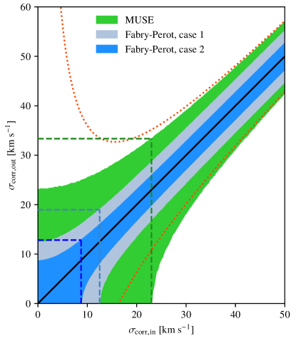
Figure 23: Range of recovered corrected velocity dispersions $\sigma_{\rm corr,out}$ as a function of the input corrected velocity dispersion $\sigma_{\rm corr,in}$ for several set-ups. The red dotted line corresponds to the analytical propagation of uncertainty of the MUSE set-up, with $\sigma_{\rm LSF}=50$ km s^-1, $\delta\sigma_{\rm obs}=5$ km s^-1, and $\delta\sigma_{\rm LSF}=1$ km s^-1. The interval determined from the Monte Carlo approach for this set-up is shown as the green area, which is partially hidden by the blue areas for visual convenience. The blue areas correspond to the Fabry-Perot set-ups, with $\sigma_{\rm LSF}=13$ km s^-1 and $\delta\sigma_{\rm LSF}=1$ km s^-1. The light blue one, which is again partially hidden by the dark blue area, corresponds to the MUSE-like uncertainties (case 1), with $\delta\sigma_{\rm obs}=5$ km s^-1, whereas the darker blue one corresponds to the most realistic hypothesis (case 2), with $\delta\sigma_{\rm obs}=2.5$ km s^-1. The black line shows the one to one relation. The three dashed lines (green, light and dark blue) correspond to the three set-ups. The vertical lines show the corrected velocity dispersion where the lower limit gets larger than zero. The horizontal lines show the corresponding upper limit, which defines the range of reliable corrected velocity dispersion.

Appendix B Impact of lines mixing to measure velocity dispersion

In crowded regions, several HII regions can contribute to the spectrum of a spatial resolution element. This is especially true for the Fabry-Perot data which have a coarser spatial resolution than the MUSE data. Theoretically, with an infinite $S/N$, lines can be separated if their shapes are perfectly known. In practice, when the line shape is not perfectly known (and assumed as Gaussian), it is not possible to asses whether their deviation from Gaussianity is due to the line shape or to a double or multiple profile, unless the lines are resolved. This happens when their separation is larger than $\sim 1.1415$ times the LSF full-width at half maximum (FWHM , Rayleigh criterion adapted to spectroscopic instruments, Namioka 1998), which corresponds to a velocity separation of $\sim 133$ km s^-1 and $\sim 34$ km s^-1 for the MUSE and the Fabry-Perot data, respectively. According to the velocity field amplitude (Fig. 5), adjacent regions can be marginally spectrally resolved with the Fabry-Perot data, but absolutely not with MUSE. In addition, if the lines have intrinsic velocity dispersions of the order of 10-20 km s^-1, they are spectrally resolved within the Fabry-Perot data whenever they are separated by at least 38-56 km s^-1, which is unlikely.

In order to measure the impact of mixing lines on the estimation of the velocity dispersion for the Fabry-Perot data, we have simulated two-components spectra with a line intensity ratio varying from 0 to 1 and with an intrinsic velocity dispersion of 15 km s^-1, which is a lower limit to the typical velocity dispersion in the warm component (see e.g. Epinat et al. 2010). In order to investigate the limit case where lines can be marginally resolved, we first set the separation between the lines to the theoretical observed FWHM of one resulting line, i.e. to 46 km s^-1. We then measured the spectrum properties with a single Gaussian fit and found that the measurement of the observed velocity dispersion of the strongest line is biased by less than 10% if the ratio of the line intensities is lower than 12%. We then performed the same exercise on a less extreme case, with a separation between the lines twice less, i.e. equals to 23 km s^-1, and found that the ratio of intensities can reach 24% before affecting the result by more than 10% (see Fig. 24). With this level of contamination, the impact on the corrected dispersion is less than 20%. As an acceptable compromise, we adopt a limit of 20% in the line intensity ratio in the analysis presented in Sect. 3.5.2. We further stress that we did not find clear evidence for multiple peaks in the Fabry-Perot spectra of selected HII regions. If multiple components exist, they should be separated by less than a small fraction of the LSF FWHM.

Figure 24: Illustration of the effect of the mix of two lines, having both an intrinsic velocity dispersion $\sigma_{\rm corr}=15$ km s^-1, and with a LSF width $\sigma_{\rm LSF}=13$ km s^-1, on the extracted velocity dispersion with two line separations: half of a single line FWHM (left) and FWHM (right). The mix of the two lines (red and blue dotted curves) with an intensity ratio of 0.2 is shown on the top panels by the black curve, whereas the single Gaussian fit is shown in dotted gray. The single line and the fitted line velocity dispersions ($2\times\sigma_{\rm obs}$) are shown as blue and gray horizontal segments, respectively. The bottom plots illustrate the variation of the relative uncertainty on both the observed (red) and corrected (blue) velocity dispersion when the line ratio varies between 0 and 1.

Appendix C Spatial contamination of adjacent regions

We aim at estimating the contribution of any neighboring region on the spectrum of a region that we wish to study. Indeed, given the high angular resolution of the VESTIGE data used to identify the HII regions ($\sim$ 0.74 arcsec), some of them are not resolved in the Fabry-Perot data ($\sim$ 2 arcsec). For any HII region, identified with an index $i$, the HIIphot software computes the flux $F_{i}$ within the region area $A_{i}$, and the effective circular full width at half-maximum, $FWHM_{i,\rm eff}$ of a 2D-Gaussian model (see Helmboldt et al. 2005). We note $\sigma_{i,\rm eff}=\frac{FWHM_{i,\rm eff}}{2\sqrt{2\log{2}}}$ the dispersion corresponding to the measured region size within the VESTIGE data. We evaluated the typical radius $r_{i}$ (in arcsecond) of each region from its measured area $A_{i}$ in square arcseconds as $r_{i}=\sqrt{A_{i}/\pi}$. Assuming that $F_{i}$ corresponds to the flux of the 2D symmetric Gaussian within $r_{i}$, we estimated for each region the total flux $F_{i,T}$ as:

$$F_{i,T}=\frac{F_{i}}{1-\exp{\left(-\frac{r_{i}^{2}}{2\sigma_{i,\rm eff}^{2}}\right)}}$$ (13)

and deduced the central intensity $I_{0,i}$ in the Fabry-Perot data as:

$$I_{0,i}=\frac{F_{i,T}}{2\pi\sigma_{i}^{2}}$$ (14)

where $\sigma_{i}$ is the observed spatial dispersion of the region within the Fabry-Perot data. Assuming that both the VESTIGE and the Fabry-Perot data PSF are well described by Gaussian functions with spatial dispersion $\sigma_{\rm V}$ and $\sigma_{\rm FP}$ respectively, we have $\sigma_{i}^{2}=\sigma_{i,\rm eff}^{2}+\sigma_{\rm FP}^{2}-\sigma_{\rm V}^{2}$.

For simplicity, we assumed that when we study one region (region 1), we measure the spectrum at its centre. We therefore needed to evaluate the intensity of any another region (region $i$) at this location. We estimated a contamination parameter of region $i$ on region 1 as the ratio of lines intensity at this location:

$$R_{1i}=\frac{I_{i}(d)}{I_{1}(0)}=\frac{F_{i,T}}{F_{1,T}}\times\frac{\sigma_{1}^{2}}{\sigma_{i}^{2}}\times\exp{\left(-\frac{d_{1i}^{2}}{2\sigma_{i}^{2}}\right)}$$ (15)

where $d_{1i}$ is the separation between the centres of the two regions.

We have also computed the background contamination in each bin associated to a given region. For this purpose we have estimated on the MUSE data the mean diffuse background surface brightness of the stellar disc in several extended regions deprived of HII regions: $\Sigma(H\alpha)$ $\sim 2\times 10^{-17}$ erg s^-1 cm^-2 arcsec^-2. We assumed this background to be constant over all regions. For each region, we have integrated this background surface brightness over the area of the associated Fabry-Perot bin $A_{i,\rm FP}$. We have also integrated the flux of the region over the bin area assuming it corresponds to the flux of a 2D-Gaussian with a dispersion $\sigma_{i}$ within a radius $r_{i,\rm FP}=\sqrt{A_{i,\rm FP}/\pi}$, and deduced a background contamination parameter as the ratio between the background flux over the region flux.

In the analysis of the kinematical properties of the HII regions presented in the paper, we have removed all regions for which the contamination parameter is larger than $R_{1i}=0.2$ for at least one neighboring region or for the background. We further excluded regions for which the barycenter of bins were further away by more than 2 arcseconds from the region centre. To conclude, with these selection criteria we expect that the velocity dispersion measurements used in the analysis are affected by less than 10%.

Appendix D Application to the data

The application of these selection criteria for the identification of the corresponding HII regions to the VESTIGE and Fabry-Perot data and the estimate of the velocity dispersion is illustrated in Fig. 25. The HIIphot pipeline identifies several HII regions in a crowded region of the galaxy on the deep VESTIGE narrow-band imaging data (green contours). The Voronoi bin with the closest barycenter in the Fabry-Perot data is identified with the black polygons for the brightest HII regions. Its size increases with the decrease of the H$\alpha$ line intensity of the region, some of which are undetected in the shallower Fabry-Perot data. For those Voronoi bins satisfying the above criteria (barycenter less than 2 arcsec away from the HII region centre given by HIIphot on the VESTIGE image, a contamination $R_{1i}$ $\leq$ 0.2), we extract a velocity dispersion measurement (regions 8, 13, 14 and 17 in Fig. 25) which is used in the analysis of the kinematical properties of the HII regions given along the text. Those not satisfying these criteria (regions 10 and 11), are not included in the analysis.

Figure 25: Lower left panel: narrow-band H$\alpha$ image of a crowded region in IC 3476. The boundaries of the individual HII regions identified by the HIIphot pipeline are indicated with the green contours. The corresponding Voronoi bins in the Fabry-Perot data are indicated with black polygons. The limiting seeing of the VESTIGE and of the Fabry-Perot data are marked with two concentric circles on the lower left corner of the image. The panels on the top and on the right of the figure show the H$\alpha$ line profiles of the velocity dispersion (in arbitrary units) of the seven selected regions indicated in the lower left panel. Of these, regions 10 and 11 do not satisfy the $R_{1i}$ $\leq$ 0.2 criterion given above, and are thus excluded from the analysis of the kinematical properties of HII regions given in the text, while regions 8, 13, 14 amd 17 are included. In each panel the red horizontal line gives the measured $\rm FWHM=2\sqrt{2\ln{2}}\times\sigma$, where $\sigma$ is the velocity dispersion.