Testing mean-field theory for jamming of non-spherical particles: Contact number, gap distribution, and vibrational density of states

Abstract

We perform numerical simulations of the jamming transition of non-spherical particles in two dimensions. In particular, we systematically investigate how the physical quantities at the jamming transition point behave when the shapes of the particle deviate slightly from the perfect disks. For efficient numerical simulation, we first derive an analytical expression of the gap function, using the perturbation theory around the reference disks. Starting from disks, we observe the effects of the deformation of the shapes of particles by the $n$-th order term of the Fourier series $\sin(n\theta)$. We show that the several physical quantities, such as the number of contacts, gap distribution, and characteristic frequencies of the vibrational density of states, show the power-law behaviors with respect to the linear deviation from the reference disks. The power-law behaviors do not depend on $n$ and are fully consistent with the mean-field theory of the jamming of non-spherical particles. This result suggests that the mean-field theory holds very generally for nearly spherical particles whose shape can be expressed by the Fourier series.

I Introduction

The jamming transition is a phenomenon that granular materials suddenly get finite rigidity at a certain density referred to as the jamming transition point $\varphi_{J}$ van Hecke (2009); Liu and Nagel (2010). Near $\varphi_{J}$, several physical quantities, such as energy, mechanical pressure, shear modulus, and contact number, exhibit the power-law behaviors O’Hern et al. (2003). This implies that the jamming transition is a critical phenomenon van Hecke (2009); Liu and Nagel (2010), such as the second-order phase transition of equilibrium systems Nishimori and Ortiz (2010).

The simplest model to study the jamming transition is the system consisting of frictionless spherical particles. The systematic numerical simulations confirmed that the critical exponents of several physical quantities do not depend on the spatial dimensions $d$ for $d\geq 2$ O’Hern et al. (2003); Vågberg et al. (2011); Charbonneau et al. (2014), while different exponents appear in a quasi-one-dimensional system Ikeda (2020). The dimensional independence of the critical exponents suggests that the exact values of the critical exponents can be calculated by considering the large dimensional limit $d\to\infty$, where the mean-field theory becomes exact Charbonneau et al. (2014); Parisi et al. (2020). This calculation has been done by using the replica method, which was originally developed for the spin-glasses, but is now widely used for many disordered systems Mézard et al. (1987); Nishimori (2001). Resultant critical exponents well agree with the numerical results in $d\geq 2$ Charbonneau et al. (2014); Parisi et al. (2020). Several other mean-field theories, such as the variational argument Wyart et al. (2005); Yan et al. (2016), effective medium theory DeGiuli et al. (2014a, b), and random matrix theory Beltukov (2015); Ikeda and Shimada (2020), are also successfully applied to derive the scaling laws of the jamming transition.

Motivated by the success of the mean-field theories for the jamming of spherical particles, we recently developed a mean-field theory of the jamming of nearly spherical particles Brito et al. (2018); Ikeda et al. (2019). The theory predicts that several physical quantities, such as the contact number and gap distribution, exhibit the singular behaviors in the limit of perfect spheres. The theoretical conjectures, however, have been confirmed mainly for the breathing particles, which are believed to have the same universality class of non-spherical particles Brito et al. (2018). It is, of course, desirable to perform a more direct test for non-spherical particles. That is the purpose of this work.

The problem is that for particles of general shape, it is numerically demanding and technically involved to calculate the gap function, which is the minimal distance between two particles and used to judge if two particles are overlapped or not Lu et al. (2015). However, since we are interested in the case where the particle shapes are close to perfect spheres, we can derive an analytic form of the gap function by using a perturbation expansion from the reference spheres Ikeda et al. (2020a, b). This allows us to perform an efficient numerical simulation.

We consider a particle system in two dimensions $d=2$. Starting from perfect disks, we deform the shapes of particles by the $n$-th order term of the Fourier series $\propto\sin(n\theta)$. We observe how this deformation affects the physical quantities, such as the contact number, gap distribution function, and characteristic frequencies of the vibrational density of states, at $\varphi_{J}$. We find that the qualitative behaviors do not depend on $n$ and fully consistent with the mean-field predictions.

The organization of the paper is as follows. In Sec. II, we summarize the previous results for jamming of frictionless spherical and non-spherical particles. In Sec. III, we introduce the model and several important physical quantities. In Sec. IV, we discuss the approximation to calculate the gap function and interaction potential. In Sec. V, we discuss the numerical algorithm to generate configurations at the jamming transition point. In Sec. VI, we check the validity of our approximation by comparing the result of our model for $n=2$ with a previous result of ellipses. In Sec. VII, we discuss the behavior of $\varphi_{J}$ and the fraction of rattles. In Sec. VIII, we discuss the scaling of the contact number at the jamming transition point. In Sec. IX, we discuss the scaling of the gap function. In Sec. X, we discuss the behavior of the vibrational density of states. Finally, in Sec. XI, we summarize the results and conclude the work.

II Previous results

We here summarize the previous numerical and theoretical results for the jamming transition of frictionless spherical and non-spherical particles.

II.1 Spherical particles

Frictionless spherical particles are isostatic at the jamming transition point in the thermodynamics limit. We first explain the concept of the isostaticity. A system is said to be isostatic if it satisfies the following condition:

$$N_{c}=N_{f},$$ (1)

where $N_{c}$ denotes the total number of constraints of the system, and $N_{f}$ denotes the total number of degrees of freedom. For $N$ frictionless spherical particles in $d$ dimensions, the total number of degrees of freedom is

$$N_{f}=Nd.$$ (2)

For a jammed configuration generated by the isotropic compression, $N_{c}$ is written as

$$N_{c}=\frac{Nz}{2}+d,$$ (3)

where $z$ denotes the number of contacts per particle. In Eq. (3), the first term $Nz/2$ represents the total number of contacts, and the second term $d$ comes from the requirement for the positive bulk modulus Goodrich et al. (2014). Therefore, if the system is isostatic, the contact number per particles is

$$z_{\rm iso}=2d-\frac{2d}{N}.$$ (4)

The systematic numerical simulations revealed that frictionless spherical particles are almost isostatic at $\varphi_{J}$, more precisely, the contact number at $\varphi_{J}$, $z_{J}\equiv z(\varphi_{J})$, is Goodrich et al. (2012)

$$z_{J}-z_{\rm iso}\propto\frac{1}{N}.$$ (5)

In particular, $z_{J}\to z_{\rm iso}$ in the thermodynamic limit $N\to\infty$ Bernal and Mason (1960); O’Hern et al. (2003).

$z$ increases on increasing the packing fraction $\varphi$. Numerical studies near $\varphi_{J}$ revealed that $z$ exhibits the following power-law behavior O’Hern et al. (2003); Goodrich et al. (2012):

$$\delta z\equiv z-z_{\rm iso}\propto\delta\varphi^{1/2},$$ (6)

where $\delta\varphi=\varphi-\varphi_{J}$. Another interesting power-law appears if one observes the gap distribution,

$$g(h)=\frac{1}{N}\sum_{i<j}\Theta(-h_{ij})\delta(h-h_{ij}),$$ (7)

where $\Theta(x)$ denotes the Heaviside step function, and $h_{ij}$ denotes the gap function defined as

$$h_{ij}=\left|\bm{r}_{i}-\bm{r}_{j}\right|-R_{i}-R_{j}.$$ (8)

Here $\bm{r}_{i}$ and $R_{i}$ denote the position and radius of the $i$-th particle, respectively. At $\varphi_{J}$ in the thermodynamic limit, $g(h)$ exhibits the power law for $h\ll 1$ Donev et al. (2005); Charbonneau et al. (2012):

$$g(h)\sim h^{-\gamma},$$ (9)

where $\gamma\approx 0.41$ Charbonneau et al. (2014, 2020). For $\varphi>\varphi_{J}$, on the contrary, the power-law is truncated at finite $h$ Charbonneau et al. (2012); Franz et al. (2017):

$$g(h)\sim\begin{cases}\delta\varphi^{-\mu\gamma}&h\ll\delta\varphi^{\mu}\\ h^{-\gamma}&h\gg\delta\varphi^{\mu}\end{cases},$$ (10)

where

$$\mu=\frac{1}{2(1-\gamma)}.$$ (11)

Figure 1: Schematic picture of $D(\omega)$. (a) $D(\omega)$ of spherical particles. (b) $D(\omega)$ of non-spherical particles.

Finally, in Fig. 1 (a), we show the schematic figure of the vibrational density of states near $\varphi_{J}$. $D(\omega)$ exhibits a plateau down to the characteristic frequency $\omega_{*}$. $\omega_{*}$ exhibits the following power-law behavior O’Hern et al. (2003); Wyart et al. (2005):

$$\omega_{*}\sim\delta z\sim\delta\varphi^{1/2}.$$ (12)

Several mean-field theories, such as the variational argument Yan et al. (2016); Wyart et al. (2005), effective medium theory DeGiuli et al. (2014a, b), and replica method Charbonneau et al. (2014); Franz et al. (2017), have been successful in reproducing the above scaling behaviors of the jamming of frictionless spherical particles. This motivates us to develop the mean-field theories for the jamming of non-spherical particles, which we shall discuss in the next subsection.

II.2 non-spherical particles

The vibrational argument predicts the same scaling laws as Eqs. (6) and (12), for a system satisfying the isostaticity Eq. (1) at $\varphi_{J}$ Yan et al. (2016). The same argument holds even for non-spherical particles. For instance, frictionless dimers become isostatic at $\varphi_{J}$ Schreck et al. (2010), and a systematic numerical simulation indeed confirmed the same scaling laws as spherical particles Shiraishi et al. (2019, 2020). More generally, for non-spherical particles consisting of spherical particles, such as dimers, trimers, …, $n$-mers, one can show that the systems are isostatic at $\varphi_{J}$ (see Appendix. A for a theoretical argument).

On the contrary, the deformation from the perfect sphere (or dimer, trimer, …), in general, breaks the isostaticity. For instance, frictionless ellipsoids Donev et al. (2004, 2007); Zeravcic et al. (2009); Mailman et al. (2009); Schreck et al. (2010, 2012), spherocylinders Williams and Philipse (2003); Blouwolff and Fraden (2006); Azéma and Radjaï (2010); Marschall and Teitel (2018), superballs Jiao et al. (2010), superellipsoids Delaney and Cleary (2010), and circulo-polygons VanderWerf et al. (2018) have been known to be hypostatic $N_{c}<N_{f}$ at $\varphi_{J}$. In the previous works, we have constructed the mean-field theories and derived the scaling laws for non-spherical particles, which are hypostatic at $\varphi_{J}$ Brito et al. (2018); Ikeda et al. (2019, 2020a). Below we summarize the main results.

The diameter $R$ of a non-spherical particle depends on the direction $\bm{n}$. We shall write $R$ as

$$R(\bm{n},\Delta)=R_{0}\left(1+\Delta F(\bm{n})\right),$$ (13)

where $R_{0}$ denotes the radius of the reference sphere, $\Delta$ represents the linear deviation from the reference sphere, and $F(\bm{n})$ characterizes the particle shape. The mean-field theory predicts that for $\Delta\ll 1$, the contact number at $\varphi_{J}$ behaves as

$$\delta z_{J}=z_{J}(\Delta)-z_{\rm iso}\propto\Delta^{1/2},$$ (14)

and $g(h)$ behaves as

$$g(h)\sim\begin{cases}\Delta^{-\mu\gamma}&h\ll\Delta^{\mu}\\ h^{-\gamma}&h\gg\Delta^{\mu}\end{cases}.$$ (15)

In Fig. 1, we also show the schematic picture of $D(\omega)$ of non-spherical particles. As in the case of spherical particles, $D(\omega)$ exhibits a plateau down to $\omega_{*}$. In addition, $D(\omega)$ of non-spherical particles has two additional peaks at $\omega_{0},\omega_{1}\ll\omega_{*}$. The characteristic frequencies exhibit the power-law behaviors:

$$\omega_{0}\sim\Delta^{1/2}\delta\varphi^{1/2},\ \omega_{1}\sim\Delta,\ \omega_{*}\sim\Delta^{1/2}.$$ (16)

In particular, at $\varphi_{J}$, we get

$$\omega_{0}=0,\ \omega_{1}\sim\Delta,\ \omega_{*}\sim\Delta^{1/2}.$$ (17)

This suggests that the modes in the lowest band become zero modes at $\varphi_{J}$. These zero modes are consequence of the hypostaticity $N_{c}<N_{f}$ and referred to as the quartic modes Mailman et al. (2009). Eqs. (14), (15), and (17) imply that increasing $\Delta$ at $\varphi_{J}$ causes the same results as increasing $\delta\varphi$ of spherical particles.

So far, Eq. (14) has been checked only for systems with small system size $N=100$, where the power-law is barely visible Brito et al. (2018), Eq. (15) has not been checked for non-spherical particles, and Eq. (17) has been checked only for ellipsoids Zeravcic et al. (2009). The purpose of this work is to test the mean-field predictions for general shapes of non-spherical particles at $\varphi_{J}$.

III Settings

Here we introduce the model and several important physical quantities.

III.1 Model

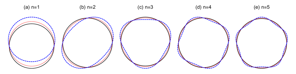
Figure 2: Particle shapes for various $n$ and $\Delta$. Black solid, red dotted, and blue dashed lines denote polar plots of $R_{i}(\theta)/R_{i}^{0}=1+\Delta F_{n}(\theta)$ for $\Delta=0$, $0.1$, and $0.3$, respectively.

We consider a two dimensional system consisting of $N$ non-spherical particles. The radius of a non-spherical particle depends on its angle $\theta\in[0,2\pi)$. We shall write the radius of the $i$-th particle as

$$R_{i}(\theta)=R_{i}^{0}\left[1+\Delta F(\theta)\right],$$ (18)

where $R_{i}^{0}$ denotes the radius of the reference disk defined by

$$R_{i}^{0}=\frac{1}{2\pi}\int_{0}^{2\pi}d\theta R_{i}(\theta).$$ (19)

$\Delta$ represents the linear deviation from the reference disk, and the function $F(\theta)$ characterizes the particle shape. $F(\theta)$ satisfies

$$\int_{0}^{2\pi}d\theta F(\theta)=0.$$ (20)

Since $F(\theta)$ is a periodic function, it is natural to express $F(\theta)$ by the Fourier series as

$$F(\theta)=\sum_{n=1}^{\infty}a_{n}\sin(n\theta+b_{n}),$$ (21)

where the constant term does not appear due to Eq. (20). Starting from the reference disk $R_{i}(\theta)=R_{i}^{0}$, we want to investigate how the $n$-th term of the Fourier series perturbs the physical quantities at $\varphi_{J}$. For this purpose, we shall consider the following functional form of $R_{i}(\theta)$:

$$R_{i}(\theta)=R_{i}^{0}\left[1+\Delta F_{n}(\theta)\right],$$ (22)

$$F_{n}(\theta)=\frac{\sin(n\theta)}{n}.$$ (23)

When $\Delta=0$, the $i$-th particle is, of course, a disk of the radius $R_{i}(\theta)=R_{i}^{0}$. On increasing $\Delta$, the shape of the $i$-th particle gradually deviates from the reference disk. In Fig. 2, we illustrate the corresponding particle shape for various $n$ and $\Delta$.

III.2 Volume fraction

We define the volume fraction $\varphi$ as

$$\varphi=\frac{\sum_{i=1}^{N}S_{i}}{L^{2}},$$ (24)

where $L$ denotes the linear distance of the system, and $S_{i}$ denotes the surface of the $i$-th particle calculated as

$$S_{i}=\int_{0}^{2\pi}d\theta\int_{0}^{R_{i}(\theta)}rdr=\frac{(R_{i}^{0})^{2}}{2}\int_{0}^{2\pi}d\theta\left[1+\Delta F_{n}(\theta)\right]^{2}.$$ (25)

III.3 Asphericity

For a particle of general shape, it is not always straightforward to find out the parameter corresponding to the linear deviation from the reference disk $\Delta$. It is sometimes convenient to use the asphericity:

$$A_{i}=\frac{P_{i}^{2}}{4\pi S_{i}},$$ (26)

where $P_{i}$ denotes the perimeter calculated as

$$P_{i}=\int_{0}^{2\pi}d\theta\sqrt{R_{i}(\theta)^{2}+\left(\frac{dR_{i}(\theta)}{d\theta}\right)^{2}}d\theta.$$ (27)

$A_{i}$ is calculated straightforwardly for particles of any shape. Furthermore, it is possible to derive the scaling relation between $A_{i}$ and $\Delta$, as follows. $A_{i}$ takes the minimal value $A_{i}=1$ for a disk $\Delta=0$, and $A_{i}>1$ for a non-disk $\Delta\neq 0$. Therefore, we get

$$A_{i}(\Delta)=1+\frac{\Delta^{2}}{2}A_{i}^{\prime\prime}(\Delta)$$ (28)

$$\to\Delta\propto(A_{i}-1)^{1/2},$$ (29)

where the linear order term does not appear, as $A_{i}(\Delta)$ has a minimum at $\Delta=0$. Eq. (29) allows to convert the scaling laws for $\Delta$ Eqs. (14,15,16) to that for $A_{i}$ Ikeda et al. (2020a). By substituting Eq. (22) into Eq. (26), one can see that $A_{i}$ does not depend on $i$, $A_{i}=A$. For $\Delta\ll 1$, we get

$$A \approx 1+\frac{\Delta^{2}}{2\pi}\int d\theta\left(F_{n}^{\prime}(\theta)^{2}-F_{n}(\theta)^{2}\right)$$ (30)

$$=1+\frac{\Delta^{2}}{2}\left(1-\frac{1}{n^{2}}\right).$$ (31)

Note that $O(\Delta^{2})$ order term vanishes for $n=1$. This means that the $n=1$ Fourier component only causes the translation of a particle for the lowest order correction Tarama et al. (2013), as illustrated in Fig. 2 (a). Hereafter we only consider $n>1$. Later, we use Eq. (31) to compare our result with the previous work of ellipsoids.

IV Interaction potential

We consider the harmonic potential O’Hern et al. (2003):

$$V_{N}=\sum_{i<j}\frac{h_{ij}^{2}}{2}\Theta(-h_{ij}),$$ (32)

where $\Theta(x)$ denotes the Heaviside step function, and $h_{ij}$ denotes the gap function, which is the minimal distance between particles $i$ and $j$. In general, it is a non-trivial task to calculate $h_{ij}$ for general shapes of non-spherical particles. Since we are interested in the scaling behaviors for $\Delta\ll 1$, we calculate $h_{ij}$ by using the first order expansion w.r.t $\Delta$, see Appendix. B for details of the calculation. After some manipulations, we get

$$h_{ij} =h_{ij}^{(1)}+O(\Delta^{2}),$$ (33)

$$h_{ij}^{(1)} =\left|\bm{r}_{i}-\bm{r}_{j}\right|-R_{i}^{0}-R_{j}^{0}$$

$$-\Delta\left[R_{i}^{0}F_{n}(\theta_{i}-\theta_{ij})+R_{j}^{0}F_{n}(\theta_{j}-\theta_{ji})\right],$$ (34)

where $\bm{r}_{i}=\{x_{i},y_{i}\}$ denotes the position of the $i$-th particle, $\theta_{i}$ denotes the direction of the $i$-th particle, and $\theta_{ij}$ denotes the relative angle of particles $i$ and $j$, namely, $\theta_{ij}={\rm atan2}(y_{j}-y_{i},x_{j}-x_{i})$, see Fig. 3.

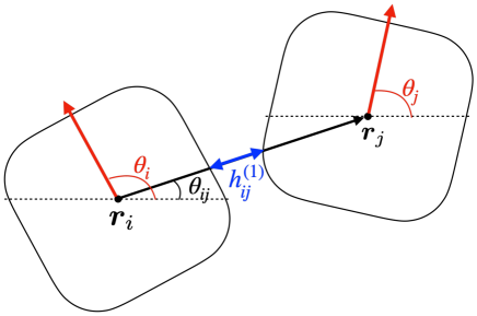
Figure 3: Definitions of $\bm{r}_{i}$, $\bm{r}_{j}$, $\theta_{i}$, $\theta_{j}$, $\theta_{ij}$, and $h_{ij}^{(1)}$. Red arrows denote particles directions, black arrow denotes the vector $\bm{r}_{j}-\bm{r}_{i}$, and dashed lines are parallel to the $x$-axis.

Hereafter, we use Eq. (34) to calculate the interaction potential. Obviously, the approximation holds only for $\Delta\ll 1$. Another limitation is that by construction, our approximation allows that two particles have at most a single contact, which is not true for particles of non-convex shapes, such as dimers, even for small aspect ratios Schreck et al. (2010).

V Numerics

We perform numerical simulations for $N$ particles confined in a $L\times L$ box. We impose the periodic boundary conditions for the both $x$ and $y$ directions. To avoid the crystallization, we consider an equimolar binary mixture: $R_{i}^{0}=0.5$ for $i=1,\dots,N/2$ and $R_{i}^{0}=0.7$ for $i=N/2+1,\dots,N$. $\varphi_{J}$ is the point at which $V_{N}$ begins to have a finite value. In practical, we define $\varphi_{J}$ as a packing fraction satisfying O’Hern et al. (2003)

$$10^{-16}<V_{N}/N<2\times 10^{-16}.$$ (35)

Here we explain how to generate configurations at $\varphi_{J}$. We first generate a random initial configuration at small packing fraction $\varphi=0.1$. Next, we slightly increase the density $\varphi\to\varphi+\varepsilon$ with $\varepsilon=10^{-3}$, and then minimize $V_{N}$ by using the FIRE algorithm, which combines the standard molecular dynamics of the Newton equation

$$m\frac{d^{2}\bm{r}_{i}}{dt^{2}}=-\frac{\partial V}{\partial\bm{r}_{i}},$$

$$I\frac{d^{2}\theta_{i}}{dt^{2}}=-\frac{\partial V}{\partial\theta_{i}},$$ (36)

with adaptive damping of the velocity Bitzek et al. (2006). We find that the FIRE converges in a reasonable time if we set $m=1$ and $I=\Delta$ so that $\ddot{\bm{r}}_{i}=O(\Delta^{0})$ and $\ddot{\theta}_{i}=O(\Delta^{0})$. We stop the FIRE algorithm when $\left(\frac{\partial V_{N}}{\partial\bm{r}_{i}}\right)^{2}+\left(\frac{\partial V_{N}}{\partial\theta}_{i}\right)^{2}<10^{-25}$, or $V_{N}/N<10^{-16}$ O’Hern et al. (2003). We repeat the above compression $\delta\varphi\to\varphi+\varepsilon$ and minimization protocols as long as $V_{N}/N\leq 10^{-16}$ after the minimization. On the contrary, if $V_{N}/N>10^{-16}$ after the minimization, we then decompress the system by changing the sign and amplitude of $\varepsilon$ as $\varepsilon\to-\varepsilon/2$. We repeat the above compression/decompression protocols by changing $\varepsilon\to-\varepsilon/2$ every time the energy crosses the threshold value $V_{N}/N=10^{-16}$. We terminates the simulation when $10^{-16}<V_{N}/N<2\times 10^{-16}$. In Fig. 4, we show configurations at $\varphi_{J}$ generated by the above algorithm.

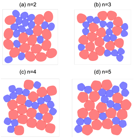
Figure 4: Configurations at $\varphi_{J}$ for $N=32$, $\Delta=0.2$ and $n=2,\dots,5$.

When calculate $z_{J}$ and $g(h)$, we remove the rattles, for which the contact number is less than $d+1=3$ O’Hern et al. (2003). To improve the statistics, we take the average for $50$ independent samples.

VI Comparison of our model and ellipses

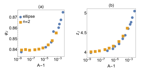
Figure 5: Comparison of ellipses and our model for $n=2$. Data for ellipses are taken from Ref. VanderWerf et al. (2018).

In this section, we compare our results with a previous numerical simulation of ellipses VanderWerf et al. (2018), where $\varphi_{J}$ and $z_{J}$ were calculated as functions of $A$. The shape of an ellipse is defined by the following equation:

$$1=\frac{x^{2}}{a^{2}}+\frac{y^{2}}{b^{2}}.$$ (37)

When the aspect ratio is close to one, say $a=R^{0}$ and $b=R^{0}(1-\varepsilon)$ with $\varepsilon\ll 1$, we get

$$R(\theta) \equiv\sqrt{x^{2}+y^{2}}\approx R^{0}\sqrt{1+2\varepsilon y^{2}}$$

$$\approx R^{0}\left[1+\varepsilon+\varepsilon\sin\left(2\theta-\frac{\pi}{2}\right)\right].$$ (38)

As the constant term and phase shift do not change the shapes of particles, Eq. (38) suggests that ellipses can be identified with our model of $n=2$ in the lowest order. In Fig. 13, we compare our result for $n=2$ and $N=512$ with that of ellipses for $N=480$ VanderWerf et al. (2018) (the finite $N$ effect is not visible in the semi-log plot.). We find a reasonable agreement for $A\sim 1$ or equivalently $\Delta\ll 1$, as expected.

VII Packing fraction and fraction of rattles

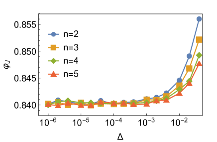
Figure 6: $\Delta$ dependence of $\varphi_{J}$ for $N=1024$.

In Fig. 6, we show the $\Delta$ dependence of $\varphi_{J}$ for $n=2,\dots,5$. On increasing of $\Delta$, $\varphi_{J}$ increases for all $n$. This is consistent with the previous numerical results of non-spherical particles, such as ellipsoids Donev et al. (2004), dimers Schreck et al. (2010), spherocylinders Williams and Philipse (2003), and circulo-polygons VanderWerf et al. (2018). The more gradual increase of $\varphi_{J}$ is observed for the larger $n$. It is interesting future work to see what will happen for much larger value of $n$. For $n\to\infty$, we expect that $\varphi_{J}$ decreases on increasing of $\Delta$, because the surface of particles becomes very rough and the system may be mapped into frictional particles of the effective friction coefficient $\mu\sim\left|\partial_{\theta}V_{N}/\partial_{\bm{r}}V_{N}\right|\sim\Delta$ Ikeda et al. (2020b).

Figure 7: $\Delta$ dependence of the fraction of rattles $f_{r}$ for $N=1024$.

In Fig. 7, we show the $\Delta$ dependence of the fraction of rattles:

$$f_{r}=\frac{N_{r}}{N},$$ (39)

where $N_{r}$ denotes the number of rattles. We find that $f_{r}$ decreases on increasing of $\Delta$ for all $n$. The similar results have been reported for ellipses and ellipsoids Donev et al. (2007).

VIII Contact number at jamming

In this section, we present our numerical results for the contact number at the jamming transition point $z_{J}\equiv z(\varphi_{J})$.

VIII.1 $N$ dependence for $n=2$

We first perform the finite size scaling analysis for $n=2$. In Fig. 8, we show $\delta z_{J}=z_{J}-z_{\rm iso}$ of our model for $n=2$ and $N=64,\dots,1024$. We find a power-law region $\delta z_{J}\sim\Delta^{1/2}$ for intermediate values of $\Delta$. The power-law region becomes wider on increasing $N$.

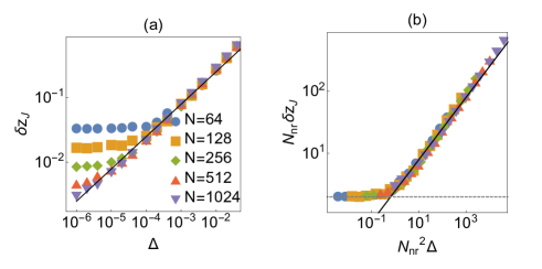
Figure 8: $\delta z_{J}$ for $n=2$ and several $N$. (a) Markers denote the numerical results. (b) Scaling plot for the same data. Black solid line and gray dashed line denote $\delta z_{J}\propto\Delta^{1/2}$ and $\delta z_{J}=2/N_{\rm nr}$, respectively

Inspired by the finite $N$ scaling analysis for frictionless spherical particles Goodrich et al. (2012), we assume the following scaling form:

$$\delta z_{J}\sim N_{\rm nr}^{-1}\tilde{z}(N_{\rm nr}^{2}\Delta),$$ (40)

where $N_{\rm nr}=N-N_{r}$ denotes the number of non-rattler particles, and

$$\tilde{z}(x)\sim\begin{cases}x^{0}&x\ll 1\\ x^{1/2}&x\gg 1\\ \end{cases}.$$ (41)

In Fig. 8 (b), we test the above scaling. A good scaling collapse confirms Eq. (40). Also, we find that $\delta z_{J}\to 2/N_{\rm nr}$ for $N_{\rm nr}^{2}\Delta\to 0$, see the dashed horizontal line in Fig. 8 (b). This means that the system has just one extra contact than the number of degrees of freedom, which is also consistent with the previous finite size analysis of frictionless disks Goodrich et al. (2012).

VIII.2 $n$ dependence for $N=1024$

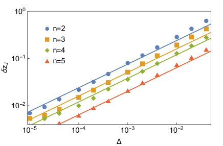
Figure 9: $\delta z_{J}$ for $N=1024$ and $n=2,\dots,5$. Markers denote the numerical results, and solid lines denote $\delta z_{J}\propto\Delta^{1/2}$.

Now we focus on the data of the largest size $N=1024$. We only show the results for $\delta z_{J}\gg 1/N$ so that the finite $N$ effects do not appear. In Fig. 9, we plot our numerical results of $\delta z_{J}$ for $n=2,\dots,5$. We find that $\delta z_{J}\propto\Delta^{1/2}$ for all $n$, which confirms the mean-field prediction Eq. (14).

IX Gap distribution

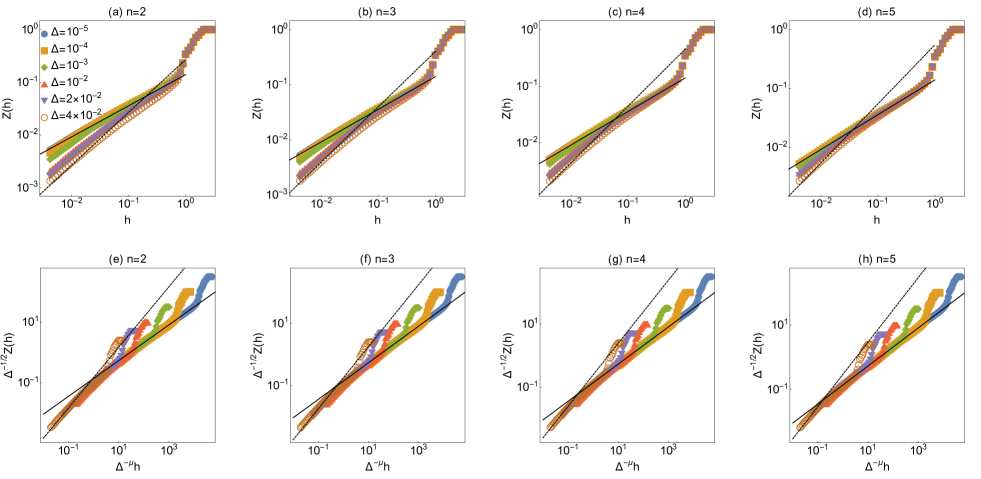
Figure 10: (a–d) $Z(h)$ for $N=1024$, and $n=2,\dots,5$. Markers denote the numerical results, solid line denotes $Z(h)\sim h^{1-\gamma}$, and dashed line denotes $Z(h)\sim h$. (e–h) Scaling plot for the same data.

In this section, we discuss the gap distribution $g(h)$ at $\varphi_{J}$. To improve the statistics, instead of $g(h)$ itself, we observe the cumulative distribution function:

$$Z(h)=\frac{\int_{0}^{h}g(h)dh}{\int_{0}^{h_{\rm cut}}g(h)dh}.$$ (42)

By definition $Z(0)=0$ and $Z(h_{\rm cut})=1$. We set $h_{\rm cut}=2$, which is large enough to observe the scaling behavior. In Fig. 10 (a–d), we show our numerical results of $Z(h)$ for $n=2,\dots,5$. We find that for small $\Delta$ and $h$, $Z(h)$ exhibits the power-law $Z(h)\sim h^{1-\gamma}$, suggesting $g(h)\sim h^{-\gamma}$. On the contrary, for large $\Delta$, $Z(h)$ exhibits the liner behavior $Z(h)\sim h$ for $h\ll 1$, suggesting $g(h)\sim h^{0}$. These results are consistent with the mean-field prediction Eq. (15).

By using Eq. (15), we can deduce the scaling form of $Z(h)$ as Ikeda et al. (2020a)

$$Z(h)\sim\Delta^{1/2}\tilde{Z}(\Delta^{-\mu}h),$$ (43)

where $\tilde{Z}(x)$ satisfies

$$\tilde{Z}(x)\sim\begin{cases}x&x\ll 1\\ x^{1-\gamma}&x\gg 1\end{cases}.$$ (44)

In Fig. 10 (e–h), we test the above equation. We find a reasonable data collapse.

X Vibrational density of states

Finally, we investigate the vibrational density of states $D(\omega)$ at $\varphi_{J}$. We define the Hessian of the interaction potential as

$$\mathcal{H}_{X_{i}Y_{j}}=\frac{\partial^{2}V_{N}}{\partial X_{i}\partial Y_{j}}=K_{X_{i}Y_{j}}+T_{X_{i}Y_{j}},$$

$$K_{X_{i}Y_{j}}=\sum_{i<j}v^{\prime\prime}(h_{ij})\frac{\partial h_{ij}}{\partial X_{i}}\frac{\partial h_{ij}}{\partial Y_{j}},$$

$$T_{X_{i}Y_{j}}=\sum_{i<j}v^{\prime}(h_{ij})\frac{\partial^{2}h_{ij}}{\partial X_{i}\partial Y_{j}},$$ (45)

where $X_{i}\in\{\bm{r}_{i},\theta_{i}\}$ and $Y_{j}\in\{\bm{r}_{j},\theta_{j}\}$. At the jamming transition point, $v^{\prime}(h_{ij})=0$, and thus

$$\mathcal{H}_{X_{i}Y_{j}}\to K_{X_{i}Y_{j}}$$

$$=\delta_{ij}\sum_{k\neq i}\Theta(-h_{ik})\frac{\partial h_{ik}}{\partial X_{i}}\frac{\partial h_{ik}}{\partial Y_{i}}+(1-\delta_{ij})\Theta(-h_{ij})\frac{\partial h_{ij}}{\partial X_{i}}\frac{\partial h_{ij}}{\partial Y_{j}}.$$ (46)

Using the eigenvalues of $H_{X_{i}Y_{j}}$, $\{\lambda_{n}\}_{n=1,\dots,3N}$, $D(\omega)$ is calculated as

$$D(\omega)=\frac{1}{3N}\sum_{n=1}^{3N}\delta(\omega-\sqrt{\lambda_{n}}).$$ (47)

As mentioned below Eq. (17), $D(\omega)$ has zero modes at $\varphi_{J}$, in addition to the trivial zero modes related to the rattler particles Mailman et al. (2009); VanderWerf et al. (2018). In practice, however, the zero modes have finite frequencies depending on the accuracy of the numerical simulation. Hereafter, we focus on the range $\omega>10^{-5}$, which is large enough to remove the zero modes.

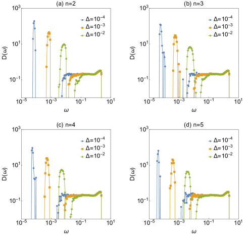
Figure 11: $D(\omega)$ for $N=1024$ and $n=2,\dots,5$. Here we do not show the zero modes.

In Fig. 11, we show our numerical results for $D(\omega)$. We find that the behavior of the high $\omega$ region ($\omega>0.1$) does not much depend on $\Delta$. On decreasing $\Delta$, $D(\omega)$ develops a plateau down to the characteristic frequency $\omega_{*}$. $D(\omega)$ has the separated band at $\omega_{1}\ll\omega_{*}$. These results are consistent with the mean-field prediction shown in Fig. 1 (b). Note that the lowest band in Fig. 1 (b) does not appear, since $\omega_{0}=0$ at $\varphi_{J}$, and we do not show the zero modes.

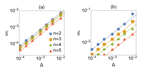
Figure 12: $\Delta$ dependence of characteristic frequencies. (a) Markers denote numerical results of $\omega_{1}$, while solid lines denote $\omega_{1}\sim\Delta$. (b) (a) Markers denote numerical results of $\omega_{*}$, while solid lines denote $\omega_{*}\sim\Delta^{1/2}$.

We want to calculate $\omega_{1}$ and $\omega_{*}$ from the numerical data of $D(\omega)$. For this purpose, we define $\omega_{1}$ as the point that maximizes $D(\omega)$, and $\omega_{*}$ as the point where $D(\omega_{*})=0.1$ in the range $\omega<0.1$. In Fig. 12, we show $\Delta$ dependence of $\omega_{1}$ and $\omega_{*}$. We find $\omega_{1}\sim\Delta$ and $\omega_{*}\sim\Delta^{1/2}$, which are consistent with the mean-field prediction, Eq. (17). The similar results have been previously reported for ellipses and ellipsoids Schreck et al. (2012); Brito et al. (2018).

XI Summary and discussions

In this work, we performed a systematic numerical investigation for the jamming of nearly spherical particles in two dimensions. Starting from perfect disks, we systematically deformed the shapes of particles by the $n$-th order term of the Fourier series $\propto\sin(n\theta)$ and observed its effects on the physical quantities at the jamming transition point. For an efficient numerical simulation, we derived an analytic formula of the gap function by using the perturbation expansion from the reference disks. By using the approximated gap function, we numerically generated configurations at the jamming transition point, and calculated the contact number, (cumulative) gap distribution, and vibrational density of states for $n=2,\dots 5$. We found the qualitatively the same scaling behaviors, which are fully consistent with the mean-field predictions, for all $n$. This means that mean-field prediction is applicable to general-shaped convex particles whose particle shape can be represented by the Fourier series.

There are still several important points that deserve further investigation. Here we give a tentative list:

• As mentioned before, our approximation does not hold for non-convex particles, such as dimers, where particles may have multiple contacts. It is important future work to extend the approximation for the gap function so as to take into account the effects of the multiple contacts.

• In this work, we investigate the physical quantities only at $\varphi_{J}$. It is of course important to investigate the behavior for $\varphi>\varphi_{J}$. For instance, the mean-field theory predicts that the shear modulus $G$ behaves as

  $$G \sim\Delta^{1/2}\tilde{G}\left(\Delta^{-1}\delta\varphi\right),$$ (48)

  where $\tilde{G}(x)\sim x$ for $x\ll 1$ and $\tilde{G}(x)\sim x^{1/2}$ for $x\gg 1$ Ikeda et al. (2020a). So far the above scaling is confirmed only for ellipsoids Ikeda et al. (2020a). It is important to test if the same scaling holds for other shapes of particles.

• The variational argument predicts that the correlation volume $v_{\rm corr}$ behaves as $v_{\rm corr}\sim\left|\delta z^{-1}\right|$ Yan et al. (2016). For frictionless spherical particles, $\delta z=0$, thus $v_{\rm corr}$ diverges at $\varphi_{J}$. On the contrary, for non-spherical particles, $\delta z\neq 0$, therefore $v_{\rm corr}$ remains finite even at $\varphi_{J}$. Recently, it has been reported that $v_{\rm corr}$ can be extracted from the participation ratio of the lowest frequency mode of the vibrational density of states Shimada et al. (2018). It is interesting to repeat the same analysis for non-spherical particles.

• In this work, we focus on a system in two dimensions $d=2$. It is important future work to extend the current approximation and analysis to higher $d$.

• The mean-field theory of non-spherical particles predicts that the replica symmetry breaking (RSB) occurs near the jamming transition point Ikeda et al. (2019), as in the case of spherical particles Charbonneau et al. (2014). It is important future work to find out the signature of the RSB for non-spherical particles by numerical simulations and experiments.

• For frictionless spherical particles, the different critical exponents appear in the quasi-one-dimensional system Ikeda (2020). It is interesting future work to repeat the similar analysis in Ref.  Ikeda (2020) for non-spherical particles.

Appendix A Isostaticity of particles consisting of spherical particles

To keep the generality, we consider $N$ particle system connected by $M$ bonds. For instance, $N/2$ dimers can be considered as $N$ spherical particles with $M=N/2$ bonds. We consider the harmonic potential:

$$V_{N}=\sum_{i<j}^{1,N}\frac{h_{ij}^{2}}{2}\Theta(-h_{ij})+k\sum_{a=1}^{M}\frac{t_{i_{a}j_{a}}^{2}}{2},$$ (49)

where

$$h_{ij}=\left|\bm{r}_{i}-\bm{r}_{j}\right|-R_{i}-R_{j},$$

$$t_{i_{a}j_{a}}=\left|\bm{r}_{i_{a}}-\bm{r}_{j_{a}}\right|-l_{i_{a}j_{a}}.$$ (50)

$\bm{r}_{i}=\{x_{1}^{i},\dots,x_{d}^{i}\}$ denotes the position, and $R_{i}$ denotes the diameter of the $i$-th particle, and $l_{i_{a}j_{a}}$ denotes the length of the $a$-th bond connecting particles $i_{a}$ and $j_{a}$.

Here we show that the system is isostatic at $\varphi_{J}$ by using the same argument for frictionless spherical particles Wyart et al. (2005); Wyart (2005).

The number of degrees of freedom of the system is

$$N_{f}=Nd.$$ (51)

At the jamming transition point, we have

$$\left|\bm{r}_{i_{\mu}}-\bm{r}_{j_{\mu}}\right|=R_{i_{\mu}}+R_{i_{\mu}}, \mu=1,\dots,N_{c},$$

$$\left|\bm{r}_{i_{a}}-\bm{r}_{j_{a}}\right|=l_{i_{a}j_{a}}, a=1,\dots,M.$$ (52)

where $N_{c}$ denotes the number of contacts, $i_{\mu}$ and $j_{\mu}$ denote particles of the $\mu$-th contact. One can find $\{\bm{r}_{i}\}_{i=1,\dots,N}$ satisfying the above equation if

$$Nd\geq N_{\rm const},$$ (53)

where

$$N_{\rm const}=N_{c}+M,$$ (54)

denotes the number of constraints at the jamming transition point. On the contrary, the force balance requires

$$\frac{\partial V_{N}}{\partial\bm{r}_{i}}=\sum_{j\neq i}\Theta(-h_{ij})h_{ij}\bm{n}_{ij}+k\sum_{a=1}^{M}t_{ij_{a}}\bm{n}_{ij_{a}}=0,$$ (55)

where $\bm{n}_{ij}$ denotes the normal vector connecting particles $i$ and $j$. This can be regarded as $Nd$ linear equations for $\{h_{i_{\mu}j_{\mu}}\}_{\mu=1,\dots,N_{c}}$ and $\{t_{i_{a}j_{a}}\}_{a=1,\dots,M}$. One can find a solution if

$$N_{c}+M\geq Nd.$$ (56)

From Eqs. (53) and (56), we get

$$N_{\rm const}=N_{f}\leftrightarrow N_{c}+M=Nd,$$ (57)

meaning that the system is isostaticity at the jamming transition point. For $N/2$ dimers, the total number of contacts is written as $N_{c}=(N/2)z_{J}/2$, leading to

$$z_{J}=4d-2,$$ (58)

which is consistent with the numerical results in $d=2$ Schreck et al. (2010); Shiraishi et al. (2019) and $d=3$ Shiraishi et al. (2020).

Appendix B Derivation of Eq. (34)

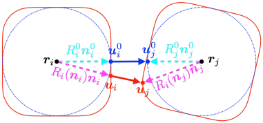
Figure 13: Schematic picture of two non-spherical particles. Red solid lines denote particles shape, and blue dashed lines denote reference disks.

We write the gap function $h_{ij}$ as

$$h_{ij} =\left|\bm{u}_{i}-\bm{u}_{j}\right|,$$ (59)

where $\bm{u}_{i}$ and $\bm{u}_{j}$ are points on the surfaces of particles $i$ and $j$ that minimize $h_{ij}$, see Fig. 13. We expand $\bm{u}_{i}$ and $\bm{u}_{j}$ from those of the reference disks as

$$\bm{u}_{i}=\bm{r}_{i}+R_{i}(\bm{n}_{i})\bm{n}_{i}=\bm{u}_{i}^{0}+\delta\bm{u}_{i},$$

$$\bm{u}_{j}=\bm{r}_{j}+R_{j}(\bm{n}_{j})\bm{n}_{j}=\bm{u}_{j}^{0}+\delta\bm{u}_{j},$$ (60)

where

$$\bm{u}_{i}^{0}=\bm{r}_{i}+R_{i}^{0}\bm{n}_{i}^{0},\ \bm{u}_{j}^{0}=\bm{r}_{j}+R_{j}^{0}\bm{n}_{j}^{0},$$

$$\delta\bm{u}_{i}=R_{i}(\bm{n}_{i})\bm{n}_{i}-R_{i}^{0}\bm{n}_{i}^{0},\delta\bm{u}_{j}=R_{j}(\bm{n}_{j})\bm{n}_{j}-R_{j}^{0}\bm{n}_{j}^{0},$$

$$\bm{n}_{i}=\frac{\bm{r}_{i}-\bm{u}_{i}}{\left|\bm{r}_{i}-\bm{u}_{i}\right|},\bm{n}_{j}=\frac{\bm{r}_{j}-\bm{u}_{j}}{\left|\bm{r}_{j}-\bm{u}_{j}\right|},$$

$$\bm{n}_{i}^{0}=\frac{\bm{r}_{i}-\bm{r}_{j}}{\left|\bm{r}_{i}-\bm{r}_{j}\right|},\bm{n}_{j}^{0}=-\bm{n}_{i}^{0},$$ (61)

see Fig. 13. $R_{i}(\bm{n}_{i})$ denotes the radius of particle $i$ along the direction $\bm{n}_{i}$. In particular,

$$R_{i}(\bm{n}_{i}^{0})=R_{i}^{0}\left[1+\Delta F(\theta_{i}-\theta_{ij})\right],$$ (62)

where $\theta_{i}$ denotes the direction of particle $i$, $\theta_{ij}$ denotes the relative angle between particles $i$ and $j$, see Fig. 3. For $\Delta\ll 1$, we can expand $h_{ij}$ w.r.t $\Delta$ as

$$h_{ij} =\left|\bm{u}_{i}-\bm{u}_{j}\right|=h_{ij}^{0}+\bm{n}_{i}^{0}\cdot\left(\delta\bm{u}_{i}-\delta\bm{u}_{j}\right)+O(\delta\bm{u}_{i}^{2},\delta\bm{u}_{j}^{2})$$

$$=h_{ij}^{0}+R_{i}^{0}-R_{i}(\bm{n}_{i})+R_{j}^{0}-R_{j}(\bm{n}_{j})+O(\Delta^{2})$$

$$=h_{ij}^{0}-\Delta\left[R_{i}^{0}F(\theta_{i}-\theta_{ij})+R_{j}^{0}F(\theta_{j}-\theta_{ji})\right]+O(\Delta^{2}),$$ (63)

where we used $\bm{n}_{i}^{0}\cdot\bm{n}_{i}=1+O(\Delta^{2})$, and $R_{i}(\bm{n}_{i})=R_{i}(\bm{n}_{i}^{0})+O(\Delta^{2})$. $h_{ij}^{0}$ denotes the gap function of the reference disks:

$$h_{ij}^{0}=\left|\bm{u}_{i}^{0}-\bm{u}_{j}^{0}\right|=\left|\bm{r}_{i}-\bm{r}_{j}\right|-R_{i}^{0}-R_{j}^{0}.$$ (64)

References

- van Hecke (2009) M. van Hecke, Journal of Physics: Condensed Matter 22, 033101 (2009).
- Liu and Nagel (2010) A. J. Liu and S. R. Nagel, Annu. Rev. Condens. Matter Phys. 1, 347 (2010).
- O’Hern et al. (2003) C. S. O’Hern, L. E. Silbert, A. J. Liu, and S. R. Nagel, Phys. Rev. E 68, 011306 (2003).
- Nishimori and Ortiz (2010) H. Nishimori and G. Ortiz, Elements of phase transitions and critical phenomena (OUP Oxford, 2010).
- Vågberg et al. (2011) D. Vågberg, D. Valdez-Balderas, M. Moore, P. Olsson, and S. Teitel, Physical Review E 83, 030303 (2011).
- Charbonneau et al. (2014) P. Charbonneau, J. Kurchan, G. Parisi, P. Urbani, and F. Zamponi, Nature communications 5, 1 (2014).
- Ikeda (2020) H. Ikeda, Phys. Rev. Lett. 125, 038001 (2020).
- Parisi et al. (2020) G. Parisi, P. Urbani, and F. Zamponi, Theory of simple glasses: exact solutions in infinite dimensions (Cambridge University Press, 2020).
- Mézard et al. (1987) M. Mézard, G. Parisi, and M. Virasoro, Spin glass theory and beyond: An Introduction to the Replica Method and Its Applications, Vol. 9 (World Scientific Publishing Company, 1987).
- Nishimori (2001) H. Nishimori, Statistical physics of spin glasses and information processing: an introduction, 111 (Clarendon Press, 2001).
- Wyart et al. (2005) M. Wyart, L. E. Silbert, S. R. Nagel, and T. A. Witten, Physical Review E 72, 051306 (2005).
- Yan et al. (2016) L. Yan, E. DeGiuli, and M. Wyart, EPL (Europhysics Letters) 114, 26003 (2016).
- DeGiuli et al. (2014a) E. DeGiuli, A. Laversanne-Finot, G. Düring, E. Lerner, and M. Wyart, Soft Matter 10, 5628 (2014a).
- DeGiuli et al. (2014b) E. DeGiuli, E. Lerner, C. Brito, and M. Wyart, Proceedings of the National Academy of Sciences 111, 17054 (2014b).
- Beltukov (2015) Y. Beltukov, JETP Letters 101, 345 (2015).
- Ikeda and Shimada (2020) H. Ikeda and M. Shimada, arXiv preprint arXiv:2009.12060 (2020).
- Brito et al. (2018) C. Brito, H. Ikeda, P. Urbani, M. Wyart, and F. Zamponi, Proceedings of the National Academy of Sciences 115, 11736 (2018).
- Ikeda et al. (2019) H. Ikeda, P. Urbani, and F. Zamponi, Journal of Physics A: Mathematical and Theoretical 52, 344001 (2019).
- Lu et al. (2015) G. Lu, J. Third, and C. Müller, Chemical Engineering Science 127, 425 (2015).
- Ikeda et al. (2020a) H. Ikeda, C. Brito, and M. Wyart, Journal of Statistical Mechanics: Theory and Experiment 2020, 033302 (2020a).
- Ikeda et al. (2020b) H. Ikeda, C. Brito, M. Wyart, and F. Zamponi, Phys. Rev. Lett. 124, 208001 (2020b).
- Goodrich et al. (2014) C. P. Goodrich, S. Dagois-Bohy, B. P. Tighe, M. van Hecke, A. J. Liu, and S. R. Nagel, Phys. Rev. E 90, 022138 (2014).
- Goodrich et al. (2012) C. P. Goodrich, A. J. Liu, and S. R. Nagel, Phys. Rev. Lett. 109, 095704 (2012).
- Bernal and Mason (1960) J. Bernal and J. Mason, Nature 188, 910 (1960).
- Donev et al. (2005) A. Donev, S. Torquato, and F. H. Stillinger, Phys. Rev. E 71, 011105 (2005).
- Charbonneau et al. (2012) P. Charbonneau, E. I. Corwin, G. Parisi, and F. Zamponi, Phys. Rev. Lett. 109, 205501 (2012).
- Charbonneau et al. (2020) P. Charbonneau, E. Corwin, C. Dennis, R. D. H. Rojas, H. Ikeda, G. Parisi, and F. Ricci-Tersenghi, arXiv preprint arXiv:2011.10899 (2020).
- Franz et al. (2017) S. Franz, G. Parisi, M. Sevelev, P. Urbani, and F. Zamponi, (2017).
- Schreck et al. (2010) C. F. Schreck, N. Xu, and C. S. O’Hern, Soft Matter 6, 2960 (2010).
- Shiraishi et al. (2019) K. Shiraishi, H. Mizuno, and A. Ikeda, Phys. Rev. E 100, 012606 (2019).
- Shiraishi et al. (2020) K. Shiraishi, H. Mizuno, and A. Ikeda, arXiv preprint arXiv:2005.02598 (2020).
- Donev et al. (2004) A. Donev, I. Cisse, D. Sachs, E. A. Variano, F. H. Stillinger, R. Connelly, S. Torquato, and P. M. Chaikin, Science 303, 990 (2004).
- Donev et al. (2007) A. Donev, R. Connelly, F. H. Stillinger, and S. Torquato, Physical Review E 75, 051304 (2007).
- Zeravcic et al. (2009) Z. Zeravcic, N. Xu, A. Liu, S. Nagel, and W. van Saarloos, EPL (Europhysics Letters) 87, 26001 (2009).
- Mailman et al. (2009) M. Mailman, C. F. Schreck, C. S. O’Hern, and B. Chakraborty, Physical review letters 102, 255501 (2009).
- Schreck et al. (2012) C. F. Schreck, M. Mailman, B. Chakraborty, and C. S. O’Hern, Physical Review E 85, 061305 (2012).
- Williams and Philipse (2003) S. Williams and A. Philipse, Physical Review E 67, 051301 (2003).
- Blouwolff and Fraden (2006) J. Blouwolff and S. Fraden, EPL (Europhysics Letters) 76, 1095 (2006).
- Azéma and Radjaï (2010) E. Azéma and F. Radjaï, Phys. Rev. E 81, 051304 (2010).
- Marschall and Teitel (2018) T. Marschall and S. Teitel, Physical Review E 97, 012905 (2018).
- Jiao et al. (2010) Y. Jiao, F. H. Stillinger, and S. Torquato, Phys. Rev. E 81, 041304 (2010).
- Delaney and Cleary (2010) G. W. Delaney and P. W. Cleary, EPL (Europhysics Letters) 89, 34002 (2010).
- VanderWerf et al. (2018) K. VanderWerf, W. Jin, M. D. Shattuck, and C. S. O’Hern, Phys. Rev. E 97, 012909 (2018).
- Tarama et al. (2013) M. Tarama, A. M. Menzel, B. ten Hagen, R. Wittkowski, T. Ohta, and H. Löwen, The Journal of Chemical Physics 139, 104906 (2013).
- Bitzek et al. (2006) E. Bitzek, P. Koskinen, F. Gähler, M. Moseler, and P. Gumbsch, Physical review letters 97, 170201 (2006).
- Shimada et al. (2018) M. Shimada, H. Mizuno, M. Wyart, and A. Ikeda, Physical Review E 98, 060901 (2018).
- Wyart (2005) M. Wyart, arXiv preprint cond-mat/0512155 (2005).