Active Feature Selection for the Mutual Information Criterion

Abstract

We study active feature selection, a novel feature selection setting in which unlabeled data is available, but the budget for labels is limited, and the examples to label can be actively selected by the algorithm. We focus on feature selection using the classical mutual information criterion, which selects the $k$ features with the largest mutual information with the label. In the active feature selection setting, the goal is to use significantly fewer labels than the data set size and still find $k$ features whose mutual information with the label based on the entire data set is large. We explain and experimentally study the choices that we make in the algorithm, and show that they lead to a successful algorithm, compared to other more naive approaches. Our design draws on insights which relate the problem of active feature selection to the study of pure-exploration multi-armed bandits settings. While we focus here on mutual information, our general methodology can be adapted to other feature-quality measures as well. The code is available at the following url:
https://github.com/ShacharSchnapp/ActiveFeatureSelection.

1 Introduction

Feature selection is the task of selecting a small number of features which are the most predictive with respect to the label. Filter methods for feature selection (see, e.g., Guyon et al. 2008) attempt to select the best features without committing to a specific model or task. We focus here on the classical mutual-information filter method, which selects the features with the largest mutual information with the label.

In the standard feature selection setting, the mutual information of each feature with the label is estimated based on a fully-labeled data set. In this work, we study a novel active setting, in which only the unlabeled data is readily available, and there is a limited budget for labels, which may be obtained upon request. In this setting, the feature selection algorithm can iteratively select an example from the data set and request its label, while taking into account in its decision all the labels obtained so far. The goal is to use significantly fewer labels than the data set size and still find $k$ features whose mutual information with the label based on the entire data set is large. This is the analog, for the feature-selection task, of the active learning setting, first proposed in Cohn, Atlas, and Ladner (1994); McCallum and Nigam (1998), which addresses classification tasks.

Feature selection in such an active setting is useful in applications characterized by a preliminary stage of feature selection with expensive labels but readily available features, followed by a deployment stage in which only a few features can be collected for each example. For instance, consider developing a medical protocol which can only use a small number of features, so that patient intake is resource efficient. The goal during protocol design is to select the most informative patient attributes with respect to a target label, such as the existence of a life-threatening condition. In the preliminary study, it is possible to collect a large number of features about a cohort of patients, but identifying the condition of the patient (the label) with a high accuracy may require paying trained specialists. By using an active feature selection algorithm which requires only a small number of labels, the labeling cost at the design stage can be controlled.

As a second example, consider a design/deploy scenario of a computer system which trains classifiers online. The online system handles large volumes, and thus cannot measure all possible features. Therefore, at the design stage, a small number of features must be selected, which will be the only ones collected later by the deployed system. The feature selection process is performed on an offline system, and therefore does not have easy access to labels, but it does allow collecting all the features for the unlabeled feature selection data set, since it handles smaller volumes of data. As a concrete example, consider a web-server which needs to quickly decide where to route client requests, by predicting the resource type that this client session will later use. In the live system, it is easy to collect the true labels downstream and feed them to the training algorithm. However, the server is limited in the number of features it can retrieve for each request, due to bounded communication with the client. On the other hand, in the design stage, there is no limit to communicating with the client, due to the smaller processing volumes. However, simulating the live process in order to identify the label is expensive, since the databases are not local.

Our goal is then to interactively select examples to label from the feature selection data set, and to then use these labeled examples to select $k$ features which have a high mutual information with the label. If the budget for labels is limited, a naive approach is to label a random subset of the unlabeled data set, and to then select the top-ranking features according to this sub-sample. Our main contribution is a practical algorithm that selects the examples to label using a smart interactive procedure. This results in selecting features of a higher quality, that is, features with a larger (true) mutual information with the label. Our design draws on insights relating the problem of active feature selection to the study of pure-exploration of multi-armed bandits (Antos, Grover, and Szepesvári 2008; Carpentier et al. 2011; Chen et al. 2014; Garivier and Kaufmann 2016), which we elaborate on below. While we focus here on mutual information, our general methodology can be adapted to other feature-quality measures, an extension that we leave for future work.

Paper structure.

Related work is discussed in Section 2. Section 3 presents the formal setting and notation. In Section 4, we discuss estimating the quality of a single feature is discussed; the solution is an important ingredient in the active feature selection algorithm, which is then presented in Section 5. Experiments are reported in Section 6. We conclude in Section 7. Full experiment results can be found in the appendices.

2 Related work

Feature selection for classification based on a fully labeled sample is a widely studied task. Classical filter methods (see, e.g., Guyon et al. 2008) select features based on a quality measure assigned to each feature. This approach does not take into account possible correlations between features, which is in general a computationally hard problem (Amaldi and Kann 1998). Nonetheless, such filter methods are practical and popular due to their computational tractability. The most popular quality measures estimate the predictive power of the feature with respect to the label, based on the labeled sample. Two popular such measures are mutual information and the Gini index (see, e.g., Hastie, Tibshirani, and Friedman 2001; Guyon et al. 2008; Sabato and Shalev-Shwartz 2008). A different approach is that of the Relief algorithm (Kira and Rendell 1992), which selects features that distinguish similar instances with different labels.

We are not aware of works on feature selection in the active setting studied here. Previous works (Liu et al. 2003; Liu, Motoda, and Yu 2004) propose to use selective sampling to improve the accuracy of the Relief feature selection algorithm within a limited run time. However, they use the labels of the entire data set, and so they do not reduce the labeling cost. Alternatively, one might consider using active learning algorithms which output sparse models to actively select features. The theory of such algorithms has been studied for learning half-spaces under specific distributional assumptions (Zhang 2018). However, we are not aware of practical active learning algorithms for a given sparsity level, which would allow performing joint active learning and feature selection using a limited label budget.

In this work, we show a connection between the active feature selection problem and exploration-only multi-armed bandit settings. A problem of uniformly estimating the means of several random arms with a small number of arm pulls is studied in Antos, Grover, and Szepesvári (2008) and in Carpentier et al. (2011). In Garivier and Kaufmann (2016), a proportion-tracking approach for optimal best-arm identification is proposed. In Chen et al. (2014), the setting of combinatorial pure exploration is studied, in which the goal is to find a subset of arms with a large total quality, using a small number of arm pulls. We discuss these works in more detail in the relevant contexts throughout the paper.

3 Setting and notations

For an integer $i$, denote $[i]=\{1,\ldots,i\}$. We first formally define the problem of selecting the top-$k$ features based on mutual information. Let $\mathcal{D}$ be a distribution over $\mathcal{X}\times\mathcal{Y}$, where $\mathcal{X}$ is the example domain and $\mathcal{Y}$ is the set of labels. Each example $x\in\mathcal{X}$ is a vector of $d$ features $(x(1),\ldots,x(d))$. We assume for simplicity that each feature $j$ accepts one of a finite set of values $V_{j}$, and that the label $\mathcal{Y}$ is binary: $\mathcal{Y}=\{0,1\}$. Denote a random labeled example by $(\mathbf{X},Y)\sim\mathcal{D}$, where $\mathbf{X}=(X(1),\ldots,X(d))$. The quality of feature $j$ is measured by its mutual information with the label, defined as $I_{j}\mathrel{\mathop{\ordinarycolon}}=I(X(j);Y)$, equal to

$$\sum_{\begin{subarray}{c}y\in\{0,1\}\\ v\in V_{j}\end{subarray}}\!\!\!\mathbb{P}(X(j)\!\!=\!\!v,Y\!\!=\!\!y)\log(\frac{\mathbb{P}(X(j)\!\!=\!\!v,Y\!=\!y)}{\mathbb{P}(Y\!\!=\!\!y)\mathbb{P}(X(j)\!\!=\!\!v)}).$$ (1)

Given an integer $k$, The goal of the feature selection procedure is to select $k$ features with the largest mutual information with the label. In standard (non-active) feature selection, the mutual information of each feature is estimated using a labeled sample of examples. In contrast, in active feature selection, the input is an i.i.d. unlabeled sample $S\mathrel{\mathop{\ordinarycolon}}=(x_{1},x_{2},...,x_{m})$ drawn according to the marginal distribution of $\mathcal{D}$ over $\mathcal{X}$. At time step $t$, the algorithm selects an example $x_{i_{t}}$ from $S$ and requests its label, $y_{i_{t}}$, which is drawn according to $\mathcal{D}$ conditioned on $\mathbf{X}=x_{i_{t}}$. If the label of the same example is requested twice, the same label is provided again. The selection of $i_{t}$ at time step $t$ may depend on the labels obtained in previous time steps. When the budget of labels is exhausted, the algorithm outputs a set of $k$ features, with the same goal as the standard feature selection algorithm: selecting the features with the largest mutual information with the label.

If the unlabeled sample $S$ is sufficiently large, then the sample distribution of each feature $X(j)$ is sufficiently similar to the true distribution. Moreover, if all the labels for $S$ were known, as in the classical non-active setting, then the plug-in estimator for mutual information, obtained by replacing each probability value in Eq. (1) with its empirical counterpart on the full labeled sample, would be a highly accurate estimator of the true mutual information (see, e.g., Paninski 2003). Therefore, for simplicity of presentation, we assume below that the empirical distribution of each feature on the unlabeled sample is the same as the true distribution, and that the best possible choice of features would be achieved by getting the labels for the entire sample $S$, and then selecting the top-$k$ features according to their mutual information plug-in estimate on the labeled sample. The challenge in active feature selection is to approach this optimal selection as much as possible, while observing considerably fewer labels.

4 Active estimation for a single feature

A core problem for the goal of actively selecting $k$ features based on their quality, is to actively estimate the quality of a single feature. We discuss this problem and its solution, as a stepping stone to the full active feature selection algorithm, which will incorporate this solution. The quality of a single feature $j$ is $I_{j}=H(Y)-H(Y\mid X(j)),$ where $H$ is the entropy function. For $v\in V_{j}$, denote $p_{v}\mathrel{\mathop{\ordinarycolon}}=\mathbb{P}[X_{j}=v]$, $q_{v}\mathrel{\mathop{\ordinarycolon}}=\mathbb{P}[Y=1\mid X(j)=v]$. Since we are interested in estimating $I_{j}$ only for the purpose of ranking the features, it is sufficient to estimate the conditional entropy:

$$H(Y\mid X(j))\equiv\sum_{v\in V_{j}}p_{v}\cdot H(Y\mid X(j)=v)=\sum_{v\in V_{j}}p_{v}\cdot H_{b}(q_{v}),$$

where $H_{b}(q)\mathrel{\mathop{\ordinarycolon}}=q\log(1/q)+(1-q)\log(1/(1-q))$ is the binary entropy. This leads to the single-feature estimation problem, described as follows. We observe $m$ i.i.d. draws $(z_{1},\ldots,z_{m})$ from the marginal distribution of $\mathcal{D}$ over $X(j)$. At each time step $t$, the algorithm selects an index $i_{t}$ and requests the label $y_{i_{t}}\sim Y|X(j)=z_{i_{t}}$. The goal is to obtain a good plug-in estimate for $H_{j}\mathrel{\mathop{\ordinarycolon}}=H(Y|X(j))$ using the available label budget. Since the examples $z_{1},\ldots,z_{m}$ are values from $V_{j}$, selecting an index $i_{t}$ is equivalent to selecting a value in $V_{j}$, and we have $y_{i_{t}}\sim Y|X(j)=v$. As discussed in Section 3, we assume for simplicity of presentation that the data set is sufficiently large, so that $p_{v}$ for $v\in V_{j}$ can be obtained by calculating the empirical probabilities of the sample. Thus, the single-feature estimation problem can be reformulated as follows: $\{p_{v}\}_{v\in V_{j}}$ are provided as input; at each time step, the algorithm selects a value $v\in V_{j}$ and obtains one random draw of $Y\mid X(j)=v$. Note that this is possible if the data set is large enough, as we assume. When the label budget is exhausted, $H_{j}$ is estimated based on the obtained samples. Since $\{p_{v}\}$ are known, the goal of the active algorithm is to estimate $\{q_{v}\}$ to a sufficient accuracy. Let $\hat{q}_{v}$ be the empirical plug-in estimate of $q_{v}$, based on the labels obtained for the value $v$. Then the entropy estimate is $\hat{H}_{j}\mathrel{\mathop{\ordinarycolon}}=\sum_{v\in V_{j}}p_{v}H_{b}(\hat{q}_{v})$. We have thus reduced the single-feature estimation problem to the problem of estimating $\{q_{v}\}_{v\in V_{j}}$.

Previous works (Antos, Grover, and Szepesvári 2008; Carpentier et al. 2011) study uniform active estimation of the expectations of several bounded random variables, by iteratively selecting from which random variable to draw a sample. In our problem, each value $v\in V_{j}$ defines the random variable $Y\mid X(j)=v$, with expected value $q_{v}$. In our notation, these works attempt to minimize the $\ell_{\infty}$ error measure $\max_{v\in V_{j}}|q_{v}-\hat{q}_{v}|$. Given the true $q_{v}$, (Antos, Grover, and Szepesvári 2008) defines the optimal normalized static allocation, a vector $\mathbf{w}=(w(v))_{v\in V_{j}}$ which sums to $1$, such that $w(v)$ is the fraction of draws that should be devoted to value $v\in V_{j}$ to minimize the expected $\ell_{\infty}$ error. However, $\mathbf{w}$ depends on the unknown $q_{v}$ values. The static-allocation strategy of Antos, Grover, and Szepesvári (2008) tries to approach the frequencies dictated by $\mathbf{w}$ by calculating an estimate $\mathbf{\hat{w}}$ at each time step, using the plug-in estimate of $q_{v}$ from the labeled data obtained so far. Let $n^{(t)}(v)$ be the number of labels requested for $v\in V_{j}$ until time step $t$. At time step $t$, the algorithm requests a label for the value $v_{t}$ which most deviates from the desired fraction of draws as estimated by $\hat{\mathbf{w}}$. Formally, it selects $v_{t}\in\operatorname*{argmax}_{v\in V_{j}}\hat{w}(v)/n^{(t)}(v).$

In Carpentier et al. (2011), an improvement to the estimate of $\mathbf{w}$ is proposed, and shown to generate an empirically superior strategy with improved convergence bounds. This strategy replaces each plug-in estimate of $q_{v}$ in the calculation of $\mathbf{\hat{w}}$ by its upper confidence bound (UCB). The UCB of $q_{v}$ is a value $\hat{q}_{v}^{u}$ such that with a high probability over the random samples, $\hat{q}_{v}^{u}\geq q_{v}$. Intuitively, this is more robust, especially when the static allocation strategy which uses the plug-in estimates may stop querying a random variable because of a wrong estimate, and thus never recover.

The approach of Carpentier et al. (2011) can be generalized to minimizing any error measure that depends on $q_{v}$ and $\hat{q}_{v}$. We study three approaches for active single-feature estimation of the mutual information, based on three error measures. In Section 6, we report an extensive experimental comparison.

The $\ell_{\infty}$ approach.

Here, we use the algorithms of Carpentier et al. (2011) for the $\ell_{\infty}$ error measure as is, thus attempting to make all estimates accurate. However, this measure ignores the importance of each value, thus many labels could be spent on values $v$ with very small $p_{v}$.

The variance approach.

Here, we take the weights $p_{v}$ into account, by replacing the $\ell_{\infty}$ error with the variance of the weighted estimate for a budget of $B$ samples:

$$\mathrm{Var}(\sum_{v}p_{v}\hat{q}_{v})=\sum_{v}p_{v}^{2}\mathrm{Var}(\hat{q}_{v})=\sum_{v}p_{v}^{2}q_{v}(1-q_{v})/(Bw(v)).$$

Minimizing this objective subject to $\sum_{v}w(v)=1$ leads to the following static allocation:

$$w_{\mathrm{var}}(v)\propto p_{v}\sqrt{q_{v}(1-q_{v})}.$$

Here and below, the notation $w(v)\propto\alpha(v)$ for some function $\alpha$ indicates that $w(v)=\alpha(v)/\sum_{u\in V_{j}}\alpha(u)$. As in the $\ell_{\infty}$ approach, we calculate $\hat{w}_{\mathrm{var}}(v)$, the estimate of $w_{\mathrm{var}}(v)$, using UCBs. However, the property of interest here is $q_{v}(1-q_{v})$, and plugging in $\hat{q}_{v}^{u}$ instead of $q_{v}$ does not lead to a UCB on this quantity. Analogously to $\hat{q}_{v}^{u}$, let $\hat{q}_{v}^{l}$ be a lower bound on the value of $q_{v}$, which holds with a high probability. Denote the upper confidence bound of a function $f$ of $q_{v}$ based on these bounds by

$$\mathrm{UCB}(f,\hat{q}_{v}^{l},\hat{q}_{v}^{u})\mathrel{\mathop{\ordinarycolon}}=\max_{x\in[\hat{q}_{v}^{l},\hat{q}_{v}^{u}]}f(x).$$

Then, if $q_{v}\in[\hat{q}_{v}^{l},\hat{q}_{v}^{u}]$, we have $f(q_{v})\leq\mathrm{UCB}(f,\hat{q}_{v}^{l},\hat{q}_{v}^{u})$. If $f$ is monotonic increasing in $[0,{\frac{1}{2}}]$ and monotonic decreasing in $[{\frac{1}{2}},1]$, then

$$\mathrm{UCB}(f,\hat{q}_{v}^{l},\hat{q}_{v}^{u})\mathrel{\mathop{\ordinarycolon}}=\begin{cases}f({\frac{1}{2}})&\hat{q}_{v}^{l}\leq{\frac{1}{2}}\leq\hat{q}_{v}^{u},\\ f(\hat{q}_{v}^{l})&\hat{q}_{v}^{l}>{\frac{1}{2}},\\ f(\hat{q}_{v}^{u})&\text{otherwise }(\hat{q}_{v}^{u}<{\frac{1}{2}}).\end{cases}$$ (2)

This holds for $f=f_{\mathrm{var}}$, where $f_{\mathrm{var}}(x)\mathrel{\mathop{\ordinarycolon}}=x(1-x)$. Plugging this into the formula for $w_{\mathrm{var}}$ given above, we get $\hat{w}_{\mathrm{var}}(v)\propto p_{v}\sqrt{\mathrm{UCB}(f_{\mathrm{var}},\hat{q}_{v}^{l},\hat{q}_{v}^{u})}$. This approach has the advantage of simplicity. However, it is not optimized for our goal, which is to estimate the conditional entropy.

The conditional entropy approach.

Here, we set the error to the variance of the conditional entropy estimate: $\mathrm{Var}(\hat{H}_{j})\equiv\sum_{v}p_{v}^{2}\cdot\mathrm{Var}(H_{b}(\hat{q}_{v}))$. Since $H_{b}$ is a smooth function of the random variable $\hat{q}_{v}$, its variance can be approximated based on its Taylor expansion (Benaroya, Han, and Nagurka 2005). Letting $H_{b}^{\prime}$ be the derivative of $H_{b}$, and $g(x)\mathrel{\mathop{\ordinarycolon}}=\sqrt{x(1-x)}|\log(\frac{x}{1-x})|$, we have

$$\mathrm{Var}(H_{b}(\hat{q}_{v}))\approx\mathrm{Var}(\hat{q}_{v}){H^{\prime}_{b}}^{2}(q_{v})=g^{2}(q_{v})/(Bw(v)).$$

Therefore, $\mathrm{Var}(\hat{H}_{j})\approx\sum_{v}p_{v}^{2}g^{2}(q_{v})/(Bw(v))$. Minimizing the RHS subject to $\sum_{v}w(v)=1$ gives the static allocation $w_{I}(v)\propto p_{v}g(q_{v})$. Here too, we estimate $\mathbf{\hat{w}}_{I}$ using upper confidence bounds. By differentiating $g$, one can see there is a value $\phi\approx 0.083$ such that $g$ is increasing in $[0,\phi]$ and in $[{\frac{1}{2}},1-\phi]$ and decreasing in $[\phi,{\frac{1}{2}}]$ and in $[1-\phi,1]$ (see illustration in Figure 1).

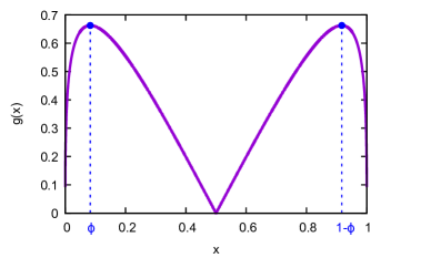
Figure 1: The function $g(x)$ defined in Active estimation for a single feature section

This implies the following upper confidence bound for $g$:

$$\mathrm{UCB}(g,\hat{q}_{v}^{l},\hat{q}_{v}^{u})=\begin{cases}g(\phi),\text{ }\phi\in[\hat{q}_{v}^{l},\hat{q}_{v}^{u}]\cup[1-\hat{q}_{v}^{u},1-\hat{q}_{v}^{l}]\\ \max\{g(\hat{q}_{v}^{l}),g(\hat{q}_{v}^{u})\},\text{ }\text{otherwise}.\end{cases}$$

Replacing $g(q_{v})$ in the definition of $w_{I}(v)$ with its upper confidence bound, we get

$$\hat{w}_{I}(v)\mathrel{\mathop{\ordinarycolon}}=\frac{\alpha(v)}{\sum_{u\in V_{j}}\alpha(u)},\text{ }\alpha(v)\mathrel{\mathop{\ordinarycolon}}=p_{v}\cdot\mathrm{UCB}(g,\hat{q}_{v}^{l},\hat{q}_{v}^{u}).$$ (3)

The two new error measures we suggested require calculating $\hat{q}_{v}^{l}$ and $\hat{q}_{v}^{u}$ for each $v\in V_{j}$. This can be done using standard closed-form concentration inequalities such as Hoeffding’s inequality (Hoeffding 1963) or Bernstein’s inequality (Bernstein 1924), as done in Carpentier et al. (2011). However, these bounds can be very loose for small sample sizes. Since $\hat{q}_{v}$ is Binomially distributed, the tightest concentration bounds are given by the Clopper-Pearson formulas (Clopper and Pearson 1934), which can be numerically calculated. Overall, we consider the following options for the single-feature estimation problem, with their abbreviations given in parenthesis: The two algorithms of Carpentier et al. (2011) for the $\ell_{\infty}$ measure, one based on Hoeffding’s inequality (MAX-H) and the other on Bernstein’s inequality (MAX-B); Static allocation strategy with $\mathbf{\hat{w}}_{\mathrm{var}}$, with each of the concentration inequalities (VAR-H, VAR-B, VAR-CP); Static allocation strategy with $\mathbf{\hat{w}}_{I}$, with each of the concentration inequalities (I-H, I-B, I-CP). In addition, we consider a naive baseline which allocates the labels proportionally to $p_{v}$ (PROP). Our experiments, reported in Section 6, show that I-CP is distinctly the most successful alternative. Indeed, it is the most tailored for the estimation task at hand. In the next section, we describe the full active feature selection algorithm, which incorporate the single-feature allocation strategy as a component.

5 The active feature selection algorithm

The active feature selection algorithm attempts to select $k$ features with the largest mutual information with the label. Naively, one could estimate $H_{j}$ separately for each of the features using the best single-feature estimation strategy, as described in Section 4. However, this would cause several issues. First, using each label for estimating only a single feature is extremely wasteful. Indeed, the label budget might even be smaller than the number of features. On the other hand, selecting the example to label based on several features may induce a sampling bias. In addition, not all features are as likely to be a part of the output top-$k$ list. This should be taken into account when selecting examples. Our approach mitigates these issues, and indeed performs well in practice, as demonstrated in Section 6.

The general framework is as follows. We define a score $\mathrm{score}(x,F)$ for each example $x\in S$ and feature subset $F\subseteq[d]$. The score estimates the utility of labeling the example $x$ in improving the entropy estimates of the features in $F$. In each iteration $t$, we calculate a feature subset $F^{(t)}\subseteq[d]$ based on the information gathered so far, and select an example $x$, out of those not labeled yet, which maximizes $\mathrm{score}(x,F^{(t)})$. We first discuss the calculation of the subset $F^{(t)}$; thereafter, we present our proposed score. To set $F^{(t)}$, we take inspiration from the problem of Combinatorial Pure Exploration (CPE) of multi-armed bandits (Chen et al. 2014). In this problem, the goal is to select a set of reward distributions (arms) that maximizes the total expected reward, by interactively selecting which distribution to sample at each step. A special case of this problem is the top-$k$ arm-selection problem (Kalyanakrishnan and Stone 2010), where the selected set of arms must be of size $k$. The CPE problem does not directly map to the active feature-selection problem, since in CPE, each step provides information about a single arm, while in active feature-selection, each label provides information about all the features. Nonetheless, a shared challenge is to decide which arms/features to consider in each sampling round; That is, how to set $F^{(t)}$.

1:Unlabeled sample $S=(x_{1},\ldots,x_{m})$, number of features to select $k$, confidence $\delta\in(0,1)$, label budget $B$, number of iterations for testing change $\Lambda$.

2:For all $j\in[d],v\in V_{j}$, $p_{v}(j)\leftarrow\mathbb{P}_{X\sim S}[X(j)=v]$.

3:$S_{1}\leftarrow()$; $\forall j\in[d],v\in V_{j},n^{(1)}(j,v)\leftarrow 0,\hat{q}_{v}(j)\leftarrow 0$.

4:for $t\in[B]$ do

5:     For all $j\in[d]$, $\hat{H}_{j}\leftarrow\sum_{v\in V_{j}}p_{v}(j)H_{b}(\hat{q}_{v}(j)),$

6:$\qquad\hat{H}^{l}_{j}\leftarrow\sum_{v}p_{v}(j)\cdot\mathrm{LCB}(H_{b},\hat{q}_{v}^{l}(j),\hat{q}_{v}^{u}(j)),$

7:$\qquad\hat{H}^{u}_{j}\leftarrow\sum_{v}p_{v}(j)\cdot\mathrm{UCB}(H_{b},\hat{q}_{v}^{l}(j),\hat{q}_{v}^{u}(j)).$

8:     $F^{(t)}_{k}\leftarrow$ Top-$k$ features according to $\hat{H}_{1},\ldots,\hat{H}_{d}$

9:     $\forall j\in F^{(t)}_{k}$, $\tilde{H}_{j}\leftarrow\hat{H}_{j}^{l}$. $\forall j\notin F^{(t)}_{k}$, $\tilde{H}_{j}\leftarrow\hat{H}_{j}^{u}$.

10:     $\tilde{F}^{(t)}_{k}\leftarrow$ Top-$k$ features according to $\tilde{H}_{1},\ldots,\tilde{H}_{d}$.

11:     $F^{(t)}\leftarrow F^{(t)}_{k}\triangle\tilde{F}^{(t)}_{k}$     # The symmetric difference

12:     if $F$ is empty, then break from the loop.

13:     Calculate $\mathbf{\hat{w}}_{I}^{(t)}$ according to Eq. (3).

14:     $\displaystyle i_{t}\leftarrow\textstyle\operatorname*{argmax}_{x_{i}\in S\setminus S_{t}}\mathrm{score}^{(t)}(x_{i},F^{(t)}).$  # Eq. (4)

15:     Request the label $y_{i_{t}}$.

16:     $S_{t+1}\leftarrow S_{t}\circ(x_{i_{t}},y_{i_{t}})$

17:     for $j\in[d]$ set $v\mathrel{\mathop{\ordinarycolon}}=x_{i_{t}}(j)$ and do

18:         $n^{(t+1)}(j,v)\leftarrow n^{(t)}(j,v)+1$

19:         $\hat{q}_{v}(j)\!\leftarrow\!|\{i\mid\!x_{i}\!\in\!S_{t},x_{i}(j)\!=\!v,y_{i}\!=\!1\}|/n^{(t)}(j,v)$.

20:         Update $\hat{q}_{v}^{l}(j),\hat{q}_{v}^{u}(j)$ according to Clopper and Pearson (1934) with confidence parameter $\delta$.

21:     end for

22:     if $\sum_{i\in F_{k}^{(t)}}\hat{H}_{i}$ has not changed in the last $\Lambda$ iterations, break from the loop and select the remaining examples to label at random.

23:end for

24:Calculate $\hat{H}_{j}$ for all $j$ based on the labeled examples

25:Return the top-$k$ features according to $\hat{H}_{1},\ldots,\hat{H}_{d}$.

Algorithm 1 AFS: Active Feature Selection for the Mutual Information Criterion

Our algorithm sets $F^{(t)}$ by adapting the approach of Chen et al. (2014) to active feature selection, as follows: Given an estimator $\hat{H}_{j}$ for $H_{j}$, and high-probability lower and upper bounds $\hat{H}^{l}_{j}$ and $\hat{H}^{u}_{j}$ for $H_{j}$, define two sets of $k$ features. The first set, $F^{(t)}_{k}$, holds the top-$k$ features according to the estimates $\{\hat{H}_{j}\}$ (that is, the $k$ features with the smallest $\hat{H}_{j}$). The second set, $\tilde{F}^{(t)}_{k}$, holds an alternative choice of top-$k$ features: those with the smallest estimates, when the estimates for $j\in F^{(t)}_{k}$ are set to $\hat{H}_{j}^{l}$, and the estimates for $j\notin F^{(t)}_{k}$ are set to $\hat{H}_{j}^{u}$. $F^{(t)}$ is set to the symmetric difference of $F^{(t)}_{k}$ and $\tilde{F}^{(t)}_{k}$. Similarly to Chen et al. (2014), improving the estimates of these features is expected to have the most impact on the selected top-$k$ set. To calculate the required $\hat{H}_{j},\hat{H}^{l}_{j},\hat{H}^{u}_{j}$, denote $p_{v}(j)\mathrel{\mathop{\ordinarycolon}}=\mathbb{P}[X(j)=v]$. Since $H_{j}=\sum_{v}p_{v}(j)H_{b}(q_{v}(j))$, we calculate $\hat{H}_{j}$ by replacing $H_{b}(q_{v}(j))$ with $H_{b}(\hat{q}_{v}(j))$. For $\hat{H}^{u}_{j}$, replace $H_{b}(q_{v}(j))$ with $\mathrm{UCB}(H_{b},\hat{q}_{v}^{l}(j),\hat{q}_{v}^{u}(j))$, calculated via Eq. (2). For $\hat{H}^{l}_{j}$, replace $H_{b}(q_{v}(j))$ with: $\mathrm{LCB}(H_{b},\hat{q}_{v}^{l}(j),\hat{q}_{v}^{u}(j))\mathrel{\mathop{\ordinarycolon}}=\min_{x\in[\hat{q}_{v}^{l},\hat{q}_{v}^{u}]}H_{b}(x)=\min\{H_{b}(\hat{q}_{v}^{l}(j)),H_{b}(\hat{q}_{v}^{u}(j))\}.$

We now discuss the scoring function $\mathrm{score}(x,F)$. First, we define a score for an example $x$ and a single feature $j$. $\mathrm{score}(x,F)$ will aggregate these scores over $j\in F$. Denote the set of examples labeled before time step $t$ by $S_{t}$, and let $n^{(t)}(j,v)\mathrel{\mathop{\ordinarycolon}}=|\{x\in S_{t}\mid x(j)=v\}|$ be the number of examples requested so far with value $v$ in feature $j$. Based on the single-feature static allocation strategy, a naive approach would be to set the score of $x$ for feature $j$ to $\hat{w}_{I}^{(t)}(j)/n^{(t)}(j,x(j))$. However, this may cause significant sampling bias which could skew the entropy estimates, since the aggregate score may encourage labeling specific combinations of feature values, thereby biasing the estimate of $\{q_{v}\}$ for some features. While complete bias avoidance cannot be guaranteed in the general case, we propose a computationally feasible heuristic for reducing this bias. We add a correction term to the single-feature score, which rewards feature pairs that have been observed considerably less than their proportion in the data set. We do not consider larger subsets, to keep the heuristic tractable. Denote the sample proportion of examples with values $v_{1},v_{2}$ for features $j_{1},j_{2}$ by $\hat{p}(j_{1},j_{2},v_{1},v_{2})\mathrel{\mathop{\ordinarycolon}}=\mathbb{P}_{X\sim S}[X({j_{1}})=v_{1},X({j_{2}})=v_{2}]$, and the proportion of these pairs in $S_{t}$ by $\hat{p}^{(t)}(j_{1},j_{2},v_{1},v_{2})\mathrel{\mathop{\ordinarycolon}}=\mathbb{P}_{X\sim S_{t}}[X({j_{1}})=v_{1},X({j_{2}})=v_{2}].$ If the ratio between these proportions is large, this indicates a strong sampling bias for this feature pair. Denote $\rho^{(t)}\mathrel{\mathop{\ordinarycolon}}=\hat{p}/\!\max(\hat{p}^{(t)},1/|S|)$. We aggregate the ratios $\rho^{(t)}$ for the relevant pairs of features using an aggregation function denoted $\psi$, to create a correction term which multiplies the naive single-feature score, thus encouraging labeling examples with under-represented pairs. $\psi$ maps a real-valued vector to a single value that aggregates its coordinate values. A reasonable function should be symmetric and monotonic; Thus, a natural choice is a vector norm, e.g., $\ell_{1}$. Our experiments in Section 6 show that other reasonable choices work similarly well. We define the score for a given function $\psi$ as follows: At time $t$, the single-feature score of an example $x$ for feature $j$ is:

$$\mathrm{score}^{(t)}(x,j,F^{(t)})\mathrel{\mathop{\ordinarycolon}}=$$

$$\frac{\hat{w}^{(t)}(j)}{n^{(t)}(j,x(j))+1}\cdot\psi((\rho^{(t)}(j,r,x(j),x(r))_{r\in F^{(t)}\setminus\{j\}}).$$

At time step $t$, the example with the largest overall score $\mathrm{score}^{(t)}$ is selected, where the score is defined as:

$$\mathrm{score}^{(t)}(x,F^{(t)})\!=\!\psi((\mathrm{score}^{(t)}(x,j,F^{(t)}))_{j\in F^{(t)}}).$$ (4)

The full active feature selection algorithm, AFS, is given in Alg. 1. AFS gets as input an unlabeled sample of size $m$, the number of features to select $k$, a label budget $B$, and a confidence parameter $\delta$, which is used to set the lower and upper bounds $\hat{q}_{v}^{l},\hat{q}_{v}^{u}$. An additional parameter $\Lambda$ is used for a safeguard described below. AFS outputs $k$ features which are estimated to have the largest mutual information with the label. The computational complexity of the algorithm is $O(B(d+mk+k\log(d)))$.

AFS includes an additional safeguard, aimed at preventing cases in which the selection strategy of AFS leads to a strongly biased estimate of the mutual information, and the selection strategy itself is too biased to allow collecting labels that correct this estimate. AFS checks if $\sum_{i\in F_{k}^{(t)}}\hat{H}_{i}$ for the current top-$k$ features has changed in the last $\Lambda$ iterations. If it has not changed, AFS selects the remaining examples at random. This guarantees that a wrong estimate will eventually be corrected, while a correct estimate will not be harmed. This safeguard only takes effect in rare cases, but it is important for preventing catastrophic failures.

6 Experiments

We first report experiments for the single-feature estimation problem, comparing the approaches suggested in Section 4. These clearly show that the I-CP approach is preferable. Then, we report experiments on several benchmark data sets for the AFS algorithm, comparing it to three natural baselines. We further report ablation studies, demonstrating the necessity of each of the mechanisms of the algorithm. Lastly, we compare different choices of $\psi$. Python $3.6$ code for all experiments is available at: https://github.com/ShacharSchnapp/ActiveFeatureSelection. The full experiment results are reported in the appendices. All experiments can be run on a standard personal computer.

Single-feature estimation. We tested the algorithms listed in Section 4 in synthetic and real-data experiments. For the synthetic experiments, we created features with the same $p_{v}$ for all feature values. This is a favorable setting for MAX-H and MAX-B, which do not take $p_{v}$ into account. We generated two sets of synthetic experiments, with features of cardinality in $\{2,4,6,8,10\}$. In the first set, $q_{v}$ was drawn uniformly at random from $[0,{\frac{1}{2}}]$; This was repeated $5$ times for each set size, resulting in $25$ experiments. In the second set, we tested cases with extreme $q_{v}$ values. For each set size, we set $n$ values to have $q_{v}=1/2$ and the rest to $q_{v}=\alpha$, for all combinations of $\alpha\in\{0.1,0.01,0.001\}$ and $n\in\{0,1,\ldots,|V_{j}|\}$. This resulted in $95$ synthetic experiments. For the real-data experiments, we tested the $14$ features of the Adult data set (Dua and Graff 2019) with their true $p_{v}$ values. We ran each test scenario 10,000 times and calculated the average estimation error, defined as $\mathrm{err}\mathrel{\mathop{\ordinarycolon}}=|\hat{H}_{j}-H_{j}|$. We further calculated $95\%$ student-t confidence intervals. For algorithm $i$, denote its confidence interval $[\mathrm{err}^{l}_{i},\mathrm{err}^{u}_{i}]$. We say that $i$ has a “clear win” if $\mathrm{err}^{u}_{i}\leq\min_{j\neq i}\mathrm{err}^{l}_{j}$, and a “win” if $\mathrm{err}^{l}_{i}\leq\min_{j\neq i}\mathrm{err}^{u}_{j}$. Table 2 reports numbers of clear wins and wins for various budgets, for each experiment and algorithm. The I-CP approach is clearly the most successful. See Appendix A for detailed results.

Active feature selection. Our active feature selection experiments were performed on all the large data sets with binary labels and discrete features in the feature-selection repository of Li et al. (2018). In addition, we tested on the MUSK data set (Dua and Graff 2019), and on the MNIST data set (LeCun and Cortes 2010) for three pairs of digits. Data set properties are listed in Table 1. We tested feature numbers $k\in\{1,5,10,20\}$.

We compared our algorithm to three natural baselines, which differ in how they select the examples to label. In all baselines, the selected $k$ features were the ones with the largest mutual information estimate, calculated based on the selected labels. The tested baselines were:

1. RANDOM: Select the examples to label at random from the data set; This is the passive baseline, since it is equivalent to running passive feature selection based on the mutual information criterion on a random labeled sample of size $B$.

2. CORESET: Use a coreset algorithm to select the $B$ most representative examples from the data set. We used the classical Farthest-First Traversal algorithm (see, e.g., Ros and Guillaume 2017, 2020) with the Hamming distance, which is the most appropriate for categorical values.

3. DWUS: Label the examples selected by the active learning algorithm Density Weighted Uncertanty Sampling (Nguyen and Smeulders 2004), implemented in the python package libact (Yang et al. 2017).

To compare the algorithms, we calculated for each algorithm the mutual information gap between the true top-$k$ features and the selected features, calculated via $\sum_{j\in F^{*}}H_{j}-\sum_{j\in F}H_{j}$, where $F$ are the top-$k$ features based on the collected labels, and $F^{*}$ are the top-$k$ features according to the true $H_{j}$, which was calculated from the full labeled sample.

We ran each experiment $30$ times. All graphs plot the average score with $95\%$ confidence intervals. We provide in Figure 2 the graphs for three of the experiments, demonstrating the advantage of AFS over the baselines. Graphs for all experiments are provided in full in Appendix B. In all experiments, AFS performs better or comparably to the best baseline; its improvement is larger for larger values of $k$.

Table 1: Data set properties

Data set	Instances	Features	Classes
BASEHOCK	1993	4862	2
PCMAC	1943	3289	2
RELATHE	1427	4322	2
MUSK	6598	167	2
MNIST: $0$ vs $1$	14,780	784	2
MNIST: $3$ vs $5$	13,454	784	2
MNIST: $4$ vs $6$	13,700	784	2

Table 2: Single-feature synthetic experiments, reporting numbers of (clear wins, wins) for each algorithm.

Synthetic experimens with uniform $q_{v}$

Budget	PROP	MAX-H	MAX-B	VAR-H	VAR-B	VAR-CP	I-H	I-B	I-CP
50	(0, 12)	(0, 2)	(0, 3)	(0, 12)	(0, 11)	(1, 1)	(0, 12)	(0, 13)	$\mathbf{(10,23)}$
100	(0, 4)	(0, 2)	(0, 4)	(0, 4)	(0, 1)	(0, 0)	(0, 4)	(0, 4)	$\mathbf{(21,25)}$
300	(0, 4)	(0, 2)	(0, 4)	(0, 4)	(0, 1)	(0, 0)	(0, 4)	(0, 10)	$\mathbf{(15,25)}$
500	(0, 3)	(0, 2)	(0, 3)	(0, 3)	(0, 1)	(0, 0)	(0, 3)	(0, 16)	$\mathbf{(9,25)}$

Synthetic experiments with fixed $q_{v}$

Budget	PROP	MAX-H	MAX-B	VAR-H	VAR-B	VAR-CP	I-H	I-B	I-CP
50	(0, 21)	(0, 6)	(0, 7)	(0, 21)	(0, 18)	(23, 38)	(0, 21)	(0, 19)	$\mathbf{(40,68)}$
100	(0, 13)	(0, 8)	(0, 7)	(0, 13)	(0, 10)	(23, 34)	(0, 13)	(0, 13)	$\mathbf{(48,69)}$
300	(0, 17)	(0, 5)	(0, 14)	(0, 17)	(0, 3)	(23, 25)	(0, 17)	(0, 32)	$\mathbf{(39,71)}$
500	(0, 15)	(0, 6)	(0, 11)	(0, 15)	(0, 2)	(8, 11)	(0, 15)	(4, 42)	$\mathbf{(43,78)}$

Real-data experiments on the Adult data set

Budget	PROP	MAX-H	MAX-B	VAR-H	VAR-B	VAR-CP	I-H	I-B	I-CP
50	(0, 11)	(0, 1)	(0, 1)	(0, 11)	(0, 9)	(0, 6)	(0, 11)	(0, 11)	$\mathbf{(2,13)}$
100	(0, 5)	(0, 0)	(0, 0)	(0, 5)	(0, 6)	(0, 3)	(0, 6)	(0, 7)	$\mathbf{(6,14)}$
300	(0, 3)	(0, 1)	(0, 1)	(0, 3)	(0, 5)	(0, 3)	(0, 3)	(0, 8)	$\mathbf{(6,14)}$
500	(0, 5)	(0, 1)	(0, 1)	(0, 5)	(0, 4)	(0, 2)	(0, 5)	(0, 7)	$\mathbf{(5,13)}$

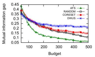
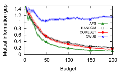
Figure 2: Some of the experiments comparing to baselines. Top: MUSK, $k=20$. Middle: MNIST, 3 vs 5, $k=20$. Bottom: RELATHE, $k=10$. See full experiment results in Appendix B.

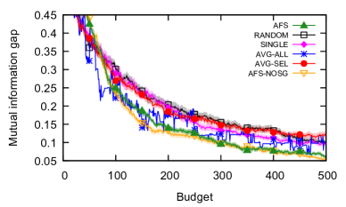
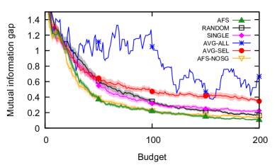
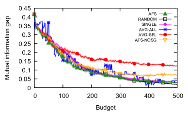
Figure 3: Some of the ablation tests. Top: MUSK, $k=20$. Middle: MNIST, 3 vs 5. Bottom: RELATHE, $k=10$. See full experiment results in Appendix C

Ablation tests. We study the necessity of the mechanisms used by AFS, by testing the following variations:

1. Select the example to label by the score of a single randomly-selected feature (SINGLE);

2. Select the example with the largest average score over all features, without a bias correction term (AVG-ALL);

3. Select the example with the largest average score over $F^{(t)}$, without a bias correction term (AVG-SEL);

4. The full AFS, with $\psi=\ell_{1}$, $\delta=0.05$, but without the safeguard (that is, $\Lambda=\infty$) (AFS-NOSG);

5. The full AFS, with $\psi=\ell_{1},\delta=0.05,\Lambda=30$ (AFS).

The value of $\Lambda$ for AFS was selected after testing the values $10,20,30,40$. The five variations above were tested on all the data sets in Table 1 for $k\in\{5,10,20\}$. Graphs for all experiments are provided in Appendix C. We provide in Figure 3 the graphs for three of the ablation tests, which show that AFS is the only algorithm that performs consistently well. We further compared our choice of $\psi\mathrel{\mathop{\ordinarycolon}}=\ell_{1}$ to other natural options: $\psi\mathrel{\mathop{\ordinarycolon}}=\ell_{\infty}$ and $\psi\mathrel{\mathop{\ordinarycolon}}=\ell_{2}$. The graphs are provided in Appendix D. We observed that in most cases, the results are similar for $\ell_{1}$ and $\ell_{2}$, while $\ell_{\infty}$ is sometimes slightly worse. Thus, while we chose $\ell_{1}$, setting $\psi\mathrel{\mathop{\ordinarycolon}}=\ell_{2}$ is also a valid choice.

7 Conclusion

We showed that actively selecting examples to label can improve the performance of feature selection for the mutual information criterion under a limited label budget. We studied the challenges involved in designing such an algorithm, and provided AFS, which improves the quality of the selected features over baselines. In future work, we will study adaptations of the suggested approach for other quality measures, such as the Gini index, and variants of the mutual information criterion that take feature correlations into account.

Appendix A Experiments: Single-feature estimation

Tables 3—A provide the full experiment results for the single-feature experiments. For each experiment, we report the average score and the confidence interval for each of the tested algorithms. Winners (as defined in Section 6) are marked in boldface. If an algorithm is the only winner in the table row, then it is a clear winner.

Table 3: Single-feature synthetic experiments; Uniform $q_{v}$; Budget of 50 labels

$[q_{v}]_{v\in V_{j}}$	PROP	MAX-H	MAX-B	VAR-H	VAR-B	VAR-CP	I-H	I-B	I-CP
$[0.01,0.5]$	$0.0405\pm 0.0002$	$0.0406\pm 0.0002$	$0.0407\pm 0.0002$	$0.0405\pm 0.0002$	$0.0403\pm 0.0002$	$\mathbf{0.0392\pm 0.0002}$	$0.0405\pm 0.0002$	$0.0404\pm 0.0002$	$0.0396\pm 0.0002$
$[0.03,0.14]$	$\mathbf{0.0692\pm 0.0005}$	$\mathbf{0.0700\pm 0.0005}$	$\mathbf{0.0698\pm 0.0005}$	$\mathbf{0.0692\pm 0.0005}$	$\mathbf{0.0700\pm 0.0005}$	$0.0708\pm 0.0005$	$\mathbf{0.0692\pm 0.0005}$	$\mathbf{0.0696\pm 0.0005}$	$\mathbf{0.0697\pm 0.0005}$
$[0.06,0.14]$	$\mathbf{0.0738\pm 0.0006}$	$\mathbf{0.0743\pm 0.0006}$	$\mathbf{0.0738\pm 0.0006}$	$\mathbf{0.0738\pm 0.0006}$	$0.0747\pm 0.0006$	$0.0788\pm 0.0006$	$\mathbf{0.0738\pm 0.0006}$	$\mathbf{0.0732\pm 0.0006}$	$0.0746\pm 0.0006$
$[0.12,0.46]$	$0.0553\pm 0.0004$	$0.0564\pm 0.0005$	$0.0555\pm 0.0004$	$0.0553\pm 0.0004$	$0.0566\pm 0.0005$	$0.0614\pm 0.0005$	$0.0553\pm 0.0004$	$0.0553\pm 0.0004$	$\mathbf{0.0531\pm 0.0004}$
$[0.49,0.26]$	$0.0397\pm 0.0003$	$0.0406\pm 0.0004$	$0.0397\pm 0.0004$	$0.0397\pm 0.0003$	$0.0401\pm 0.0004$	$0.0412\pm 0.0004$	$0.0397\pm 0.0003$	$0.0389\pm 0.0003$	$\mathbf{0.0381\pm 0.0003}$
$[0.05,0.26,0.18,0.15]$	$\mathbf{0.0704\pm 0.0005}$	$0.0734\pm 0.0005$	$0.0715\pm 0.0005$	$\mathbf{0.0704\pm 0.0005}$	$\mathbf{0.0708\pm 0.0005}$	$0.0790\pm 0.0006$	$\mathbf{0.0704\pm 0.0005}$	$\mathbf{0.0708\pm 0.0005}$	$\mathbf{0.0704\pm 0.0005}$
$[0.07,0.38,0.29,0.35]$	$0.0586\pm 0.0005$	$0.0610\pm 0.0005$	$0.0590\pm 0.0005$	$0.0586\pm 0.0005$	$0.0588\pm 0.0005$	$0.0654\pm 0.0005$	$0.0586\pm 0.0005$	$0.0586\pm 0.0005$	$\mathbf{0.0563\pm 0.0005}$
$[0.16,0.36,0.44,0.08]$	$0.0631\pm 0.0005$	$0.0652\pm 0.0005$	$0.0636\pm 0.0005$	$0.0631\pm 0.0005$	$0.0635\pm 0.0005$	$0.0704\pm 0.0005$	$0.0631\pm 0.0005$	$0.0632\pm 0.0005$	$\mathbf{0.0606\pm 0.0005}$
$[0.21,0.32,0.11,0.14]$	$\mathbf{0.0674\pm 0.0005}$	$0.0707\pm 0.0005$	$\mathbf{0.0684\pm 0.0005}$	$\mathbf{0.0674\pm 0.0005}$	$\mathbf{0.0684\pm 0.0005}$	$0.0792\pm 0.0006$	$\mathbf{0.0674\pm 0.0005}$	$\mathbf{0.0680\pm 0.0005}$	$\mathbf{0.0678\pm 0.0005}$
$[0.37,0.26,0.04,0.16]$	$0.0592\pm 0.0005$	$0.0622\pm 0.0005$	$0.0598\pm 0.0005$	$0.0592\pm 0.0005$	$0.0595\pm 0.0005$	$0.0665\pm 0.0005$	$0.0592\pm 0.0005$	$0.0593\pm 0.0005$	$\mathbf{0.0580\pm 0.0005}$
$[0.24,0.23,0.06,0.3,0.43,0.38]$	$0.0663\pm 0.0005$	$0.0712\pm 0.0005$	$0.0675\pm 0.0005$	$0.0663\pm 0.0005$	$\mathbf{0.0662\pm 0.0005}$	$0.0759\pm 0.0006$	$0.0663\pm 0.0005$	$\mathbf{0.0661\pm 0.0005}$	$\mathbf{0.0653\pm 0.0005}$
$[0.14,0.01,0.15,0.31,0.33,0.35]$	$\mathbf{0.0632\pm 0.0005}$	$0.0666\pm 0.0005$	$0.0644\pm 0.0005$	$\mathbf{0.0632\pm 0.0005}$	$0.0638\pm 0.0005$	$0.0704\pm 0.0005$	$\mathbf{0.0632\pm 0.0005}$	$0.0637\pm 0.0005$	$\mathbf{0.0626\pm 0.0005}$
$[0.14,0.38,0.46,0.44,0.13,0.36]$	$\mathbf{0.0646\pm 0.0005}$	$0.0698\pm 0.0005$	$0.0657\pm 0.0005$	$\mathbf{0.0646\pm 0.0005}$	$\mathbf{0.0644\pm 0.0005}$	$0.0745\pm 0.0005$	$\mathbf{0.0646\pm 0.0005}$	$\mathbf{0.0646\pm 0.0005}$	$\mathbf{0.0639\pm 0.0005}$
$[0.26,0.01,0.44,0.39,0.03,0.16]$	$\mathbf{0.0600\pm 0.0005}$	$0.0628\pm 0.0005$	$0.0611\pm 0.0005$	$\mathbf{0.0600\pm 0.0005}$	$\mathbf{0.0601\pm 0.0004}$	$0.0634\pm 0.0005$	$\mathbf{0.0600\pm 0.0005}$	$\mathbf{0.0605\pm 0.0005}$	$\mathbf{0.0603\pm 0.0005}$
$[0.43,0.02,0.49,0.26,0.21,0.16]$	$\mathbf{0.0612\pm 0.0005}$	$0.0666\pm 0.0005$	$0.0626\pm 0.0005$	$\mathbf{0.0612\pm 0.0005}$	$\mathbf{0.0612\pm 0.0005}$	$0.0694\pm 0.0005$	$\mathbf{0.0612\pm 0.0005}$	$\mathbf{0.0612\pm 0.0005}$	$\mathbf{0.0608\pm 0.0005}$
$[0.01,0.34,0.0,0.41,0.37,0.17,0.02,0.22]$	$\mathbf{0.0620\pm 0.0005}$	$0.0631\pm 0.0005$	$0.0632\pm 0.0005$	$\mathbf{0.0620\pm 0.0005}$	$\mathbf{0.0618\pm 0.0005}$	$0.0664\pm 0.0005$	$\mathbf{0.0620\pm 0.0005}$	$\mathbf{0.0621\pm 0.0005}$	$\mathbf{0.0619\pm 0.0005}$
$[0.26,0.16,0.24,0.31,0.2,0.47,0.31,0.46]$	$\mathbf{0.0766\pm 0.0006}$	$0.0784\pm 0.0006$	$0.0785\pm 0.0006$	$\mathbf{0.0766\pm 0.0006}$	$\mathbf{0.0768\pm 0.0006}$	$0.0892\pm 0.0006$	$\mathbf{0.0766\pm 0.0006}$	$\mathbf{0.0772\pm 0.0006}$	$\mathbf{0.0763\pm 0.0006}$
$[0.05,0.09,0.19,0.23,0.47,0.37,0.01,0.24]$	$\mathbf{0.0732\pm 0.0005}$	$0.0743\pm 0.0005$	$0.0743\pm 0.0005$	$\mathbf{0.0732\pm 0.0005}$	$\mathbf{0.0732\pm 0.0005}$	$0.0819\pm 0.0006$	$\mathbf{0.0732\pm 0.0005}$	$\mathbf{0.0731\pm 0.0005}$	$\mathbf{0.0728\pm 0.0005}$
$[0.32,0.29,0.48,0.12,0.33,0.03,0.46,0.49]$	$0.0690\pm 0.0005$	$0.0698\pm 0.0005$	$0.0698\pm 0.0005$	$0.0690\pm 0.0005$	$0.0685\pm 0.0005$	$0.0766\pm 0.0005$	$0.0690\pm 0.0005$	$\mathbf{0.0678\pm 0.0005}$	$\mathbf{0.0672\pm 0.0005}$
$[0.46,0.45,0.31,0.14,0.01,0.24,0.39,0.43]$	$\mathbf{0.0682\pm 0.0005}$	$0.0695\pm 0.0005$	$0.0695\pm 0.0005$	$\mathbf{0.0682\pm 0.0005}$	$\mathbf{0.0677\pm 0.0005}$	$0.0750\pm 0.0005$	$\mathbf{0.0682\pm 0.0005}$	$\mathbf{0.0682\pm 0.0005}$	$\mathbf{0.0674\pm 0.0005}$
$[0.11,0.03,0.01,0.25,0.41,0.47,0.4,0.17,0.0,0.36]$	$0.0709\pm 0.0005$	$0.0720\pm 0.0005$	$0.0712\pm 0.0005$	$0.0709\pm 0.0005$	$0.0708\pm 0.0005$	$0.0807\pm 0.0005$	$0.0709\pm 0.0005$	$0.0709\pm 0.0005$	$\mathbf{0.0689\pm 0.0005}$
$[0.14,0.1,0.18,0.22,0.48,0.12,0.34,0.0,0.12,0.29]$	$0.0853\pm 0.0006$	$0.0872\pm 0.0006$	$0.0880\pm 0.0006$	$0.0853\pm 0.0006$	$0.0856\pm 0.0006$	$0.1001\pm 0.0006$	$0.0853\pm 0.0006$	$0.0855\pm 0.0006$	$\mathbf{0.0834\pm 0.0006}$
$[0.26,0.31,0.23,0.3,0.27,0.3,0.24,0.02,0.49,0.16]$	$0.0847\pm 0.0006$	$0.0889\pm 0.0006$	$0.0895\pm 0.0006$	$0.0847\pm 0.0006$	$0.0848\pm 0.0006$	$0.0987\pm 0.0006$	$0.0847\pm 0.0006$	$0.0850\pm 0.0006$	$\mathbf{0.0828\pm 0.0006}$
$[0.47,0.19,0.33,0.41,0.3,0.47,0.26,0.12,0.04,0.11]$	$0.0864\pm 0.0005$	$0.0892\pm 0.0005$	$0.0890\pm 0.0005$	$0.0864\pm 0.0005$	$0.0865\pm 0.0005$	$0.0992\pm 0.0006$	$0.0864\pm 0.0005$	$0.0863\pm 0.0005$	$\mathbf{0.0843\pm 0.0005}$
$[0.28,0.27,0.11,0.45,0.26,0.47,0.09,0.44,0.14,0.42]$	$0.0866\pm 0.0006$	$0.0902\pm 0.0006$	$0.0904\pm 0.0006$	$0.0866\pm 0.0006$	$0.0867\pm 0.0006$	$0.0984\pm 0.0006$	$0.0866\pm 0.0006$	$0.0866\pm 0.0006$	$\mathbf{0.0844\pm 0.0006}$

Table 4: Single-feature synthetic experiments; Uniform $q_{v}$; Budget of 100 labels

$[q_{v}]_{v\in V_{j}}$	PROP	MAX-H	MAX-B	VAR-H	VAR-B	VAR-CP	I-H	I-B	I-CP
$[0.01,0.5]$	$0.0304\pm 0.0001$	$0.0318\pm 0.0001$	$0.0308\pm 0.0001$	$0.0304\pm 0.0001$	$0.0322\pm 0.0001$	$0.0332\pm 0.0001$	$0.0304\pm 0.0001$	$0.0288\pm 0.0001$	$\mathbf{0.0278\pm 0.0001}$
$[0.03,0.14]$	$\mathbf{0.0488\pm 0.0004}$	$\mathbf{0.0491\pm 0.0004}$	$\mathbf{0.0492\pm 0.0004}$	$\mathbf{0.0488\pm 0.0004}$	$\mathbf{0.0494\pm 0.0004}$	$0.0521\pm 0.0004$	$\mathbf{0.0488\pm 0.0004}$	$\mathbf{0.0490\pm 0.0004}$	$\mathbf{0.0491\pm 0.0004}$
$[0.06,0.14]$	$\mathbf{0.0507\pm 0.0004}$	$\mathbf{0.0511\pm 0.0004}$	$\mathbf{0.0508\pm 0.0004}$	$\mathbf{0.0507\pm 0.0004}$	$0.0519\pm 0.0004$	$0.0540\pm 0.0004$	$\mathbf{0.0507\pm 0.0004}$	$\mathbf{0.0507\pm 0.0004}$	$\mathbf{0.0508\pm 0.0004}$
$[0.12,0.46]$	$0.0387\pm 0.0003$	$0.0403\pm 0.0003$	$0.0388\pm 0.0003$	$0.0387\pm 0.0003$	$0.0404\pm 0.0003$	$0.0434\pm 0.0003$	$0.0387\pm 0.0003$	$0.0362\pm 0.0003$	$\mathbf{0.0354\pm 0.0003}$
$[0.49,0.26]$	$0.0272\pm 0.0002$	$0.0275\pm 0.0002$	$0.0274\pm 0.0002$	$0.0272\pm 0.0002$	$0.0278\pm 0.0002$	$0.0279\pm 0.0002$	$0.0272\pm 0.0002$	$0.0259\pm 0.0002$	$\mathbf{0.0253\pm 0.0002}$
$[0.05,0.26,0.18,0.15]$	$\mathbf{0.0480\pm 0.0004}$	$0.0499\pm 0.0004$	$\mathbf{0.0480\pm 0.0004}$	$\mathbf{0.0480\pm 0.0004}$	$0.0495\pm 0.0004$	$0.0560\pm 0.0004$	$\mathbf{0.0480\pm 0.0004}$	$\mathbf{0.0478\pm 0.0004}$	$\mathbf{0.0477\pm 0.0004}$
$[0.07,0.38,0.29,0.35]$	$0.0392\pm 0.0003$	$0.0405\pm 0.0003$	$0.0392\pm 0.0003$	$0.0392\pm 0.0003$	$0.0398\pm 0.0003$	$0.0450\pm 0.0003$	$0.0392\pm 0.0003$	$0.0388\pm 0.0003$	$\mathbf{0.0370\pm 0.0003}$
$[0.16,0.36,0.44,0.08]$	$0.0414\pm 0.0003$	$0.0436\pm 0.0004$	$0.0417\pm 0.0003$	$0.0414\pm 0.0003$	$0.0429\pm 0.0004$	$0.0495\pm 0.0004$	$0.0414\pm 0.0003$	$0.0412\pm 0.0003$	$\mathbf{0.0400\pm 0.0003}$
$[0.21,0.32,0.11,0.14]$	$\mathbf{0.0465\pm 0.0004}$	$0.0481\pm 0.0004$	$\mathbf{0.0466\pm 0.0004}$	$\mathbf{0.0465\pm 0.0004}$	$0.0479\pm 0.0004$	$0.0535\pm 0.0004$	$\mathbf{0.0465\pm 0.0004}$	$\mathbf{0.0465\pm 0.0004}$	$\mathbf{0.0462\pm 0.0004}$
$[0.37,0.26,0.04,0.16]$	$0.0430\pm 0.0003$	$0.0448\pm 0.0003$	$0.0432\pm 0.0003$	$0.0430\pm 0.0003$	$0.0445\pm 0.0003$	$0.0479\pm 0.0004$	$0.0430\pm 0.0003$	$0.0427\pm 0.0003$	$\mathbf{0.0420\pm 0.0003}$
$[0.24,0.23,0.06,0.3,0.43,0.38]$	$0.0414\pm 0.0003$	$0.0435\pm 0.0003$	$0.0421\pm 0.0003$	$0.0414\pm 0.0003$	$0.0417\pm 0.0003$	$0.0484\pm 0.0004$	$0.0414\pm 0.0003$	$0.0410\pm 0.0003$	$\mathbf{0.0395\pm 0.0003}$
$[0.14,0.01,0.15,0.31,0.33,0.35]$	$0.0416\pm 0.0003$	$0.0439\pm 0.0003$	$0.0420\pm 0.0003$	$0.0416\pm 0.0003$	$0.0421\pm 0.0003$	$0.0484\pm 0.0004$	$0.0416\pm 0.0003$	$0.0412\pm 0.0003$	$\mathbf{0.0401\pm 0.0003}$
$[0.14,0.38,0.46,0.44,0.13,0.36]$	$0.0381\pm 0.0003$	$0.0404\pm 0.0003$	$0.0389\pm 0.0003$	$0.0381\pm 0.0003$	$0.0388\pm 0.0003$	$0.0459\pm 0.0004$	$0.0381\pm 0.0003$	$0.0380\pm 0.0003$	$\mathbf{0.0363\pm 0.0003}$
$[0.26,0.01,0.44,0.39,0.03,0.16]$	$0.0405\pm 0.0003$	$0.0419\pm 0.0003$	$0.0406\pm 0.0003$	$0.0405\pm 0.0003$	$0.0406\pm 0.0003$	$0.0449\pm 0.0003$	$0.0405\pm 0.0003$	$0.0404\pm 0.0003$	$\mathbf{0.0391\pm 0.0003}$
$[0.43,0.02,0.49,0.26,0.21,0.16]$	$0.0387\pm 0.0003$	$0.0406\pm 0.0003$	$0.0394\pm 0.0003$	$0.0387\pm 0.0003$	$0.0391\pm 0.0003$	$0.0442\pm 0.0004$	$0.0387\pm 0.0003$	$0.0389\pm 0.0003$	$\mathbf{0.0372\pm 0.0003}$
$[0.01,0.34,0.0,0.41,0.37,0.17,0.02,0.22]$	$0.0402\pm 0.0003$	$0.0415\pm 0.0003$	$0.0409\pm 0.0003$	$0.0402\pm 0.0003$	$0.0406\pm 0.0003$	$0.0434\pm 0.0003$	$0.0402\pm 0.0003$	$0.0401\pm 0.0003$	$\mathbf{0.0389\pm 0.0003}$
$[0.26,0.16,0.24,0.31,0.2,0.47,0.31,0.46]$	$0.0459\pm 0.0004$	$0.0495\pm 0.0004$	$0.0473\pm 0.0004$	$0.0459\pm 0.0004$	$0.0463\pm 0.0004$	$0.0545\pm 0.0004$	$0.0459\pm 0.0004$	$0.0459\pm 0.0004$	$\mathbf{0.0432\pm 0.0003}$
$[0.05,0.09,0.19,0.23,0.47,0.37,0.01,0.24]$	$0.0466\pm 0.0004$	$0.0497\pm 0.0004$	$0.0476\pm 0.0004$	$0.0466\pm 0.0004$	$0.0475\pm 0.0004$	$0.0547\pm 0.0004$	$0.0466\pm 0.0004$	$0.0466\pm 0.0004$	$\mathbf{0.0453\pm 0.0003}$
$[0.32,0.29,0.48,0.12,0.33,0.03,0.46,0.49]$	$0.0413\pm 0.0003$	$0.0433\pm 0.0003$	$0.0420\pm 0.0003$	$0.0413\pm 0.0003$	$0.0415\pm 0.0003$	$0.0459\pm 0.0003$	$0.0413\pm 0.0003$	$0.0410\pm 0.0003$	$\mathbf{0.0389\pm 0.0003}$
$[0.46,0.45,0.31,0.14,0.01,0.24,0.39,0.43]$	$0.0410\pm 0.0003$	$0.0426\pm 0.0003$	$0.0416\pm 0.0003$	$0.0410\pm 0.0003$	$0.0406\pm 0.0003$	$0.0453\pm 0.0003$	$0.0410\pm 0.0003$	$0.0409\pm 0.0003$	$\mathbf{0.0383\pm 0.0003}$
$[0.11,0.03,0.01,0.25,0.41,0.47,0.4,0.17,0.0,0.36]$	$0.0440\pm 0.0003$	$0.0460\pm 0.0003$	$0.0441\pm 0.0003$	$0.0440\pm 0.0003$	$0.0438\pm 0.0003$	$0.0489\pm 0.0003$	$0.0440\pm 0.0003$	$0.0438\pm 0.0003$	$\mathbf{0.0425\pm 0.0003}$
$[0.14,0.1,0.18,0.22,0.48,0.12,0.34,0.0,0.12,0.29]$	$0.0529\pm 0.0004$	$0.0563\pm 0.0004$	$0.0535\pm 0.0004$	$0.0529\pm 0.0004$	$0.0529\pm 0.0004$	$0.0623\pm 0.0004$	$0.0529\pm 0.0004$	$0.0525\pm 0.0004$	$\mathbf{0.0516\pm 0.0004}$
$[0.26,0.31,0.23,0.3,0.27,0.3,0.24,0.02,0.49,0.16]$	$0.0506\pm 0.0004$	$0.0533\pm 0.0004$	$0.0513\pm 0.0004$	$0.0506\pm 0.0004$	$0.0507\pm 0.0004$	$0.0609\pm 0.0004$	$0.0506\pm 0.0004$	$0.0507\pm 0.0004$	$\mathbf{0.0487\pm 0.0004}$
$[0.47,0.19,0.33,0.41,0.3,0.47,0.26,0.12,0.04,0.11]$	$0.0531\pm 0.0004$	$0.0563\pm 0.0004$	$0.0542\pm 0.0004$	$0.0531\pm 0.0004$	$0.0530\pm 0.0004$	$0.0642\pm 0.0004$	$0.0531\pm 0.0004$	$0.0529\pm 0.0004$	$\mathbf{0.0511\pm 0.0004}$
$[0.28,0.27,0.11,0.45,0.26,0.47,0.09,0.44,0.14,0.42]$	$0.0526\pm 0.0004$	$0.0560\pm 0.0004$	$0.0547\pm 0.0004$	$0.0526\pm 0.0004$	$0.0525\pm 0.0004$	$0.0644\pm 0.0004$	$0.0526\pm 0.0004$	$0.0525\pm 0.0004$	$\mathbf{0.0500\pm 0.0004}$

Table 5: Single-feature synthetic experiments; Uniform $q_{v}$; Budget of 300 labels

$[q_{v}]_{v\in V_{j}}$	PROP	MAX-H	MAX-B	VAR-H	VAR-B	VAR-CP	I-H	I-B	I-CP
$[0.01,0.5]$	$0.0159\pm 0.0001$	$0.0173\pm 0.0001$	$0.0162\pm 0.0001$	$0.0159\pm 0.0001$	$0.0186\pm 0.0001$	$0.0216\pm 0.0001$	$0.0159\pm 0.0001$	$\mathbf{0.0133\pm 0.0001}$	$\mathbf{0.0134\pm 0.0001}$
$[0.03,0.14]$	$\mathbf{0.0280\pm 0.0002}$	$\mathbf{0.0281\pm 0.0002}$	$\mathbf{0.0279\pm 0.0002}$	$\mathbf{0.0280\pm 0.0002}$	$0.0288\pm 0.0002$	$0.0308\pm 0.0002$	$\mathbf{0.0280\pm 0.0002}$	$\mathbf{0.0280\pm 0.0002}$	$\mathbf{0.0280\pm 0.0002}$
$[0.06,0.14]$	$\mathbf{0.0281\pm 0.0002}$	$\mathbf{0.0284\pm 0.0002}$	$\mathbf{0.0281\pm 0.0002}$	$\mathbf{0.0281\pm 0.0002}$	$\mathbf{0.0284\pm 0.0002}$	$0.0292\pm 0.0002$	$\mathbf{0.0281\pm 0.0002}$	$\mathbf{0.0282\pm 0.0002}$	$\mathbf{0.0282\pm 0.0002}$
$[0.12,0.46]$	$0.0206\pm 0.0002$	$0.0219\pm 0.0002$	$0.0209\pm 0.0002$	$0.0206\pm 0.0002$	$0.0228\pm 0.0002$	$0.0232\pm 0.0002$	$0.0206\pm 0.0002$	$\mathbf{0.0189\pm 0.0002}$	$\mathbf{0.0188\pm 0.0002}$
$[0.49,0.26]$	$0.0149\pm 0.0001$	$0.0152\pm 0.0001$	$0.0148\pm 0.0001$	$0.0149\pm 0.0001$	$0.0153\pm 0.0001$	$0.0153\pm 0.0001$	$0.0149\pm 0.0001$	$\mathbf{0.0135\pm 0.0001}$	$\mathbf{0.0135\pm 0.0001}$
$[0.05,0.26,0.18,0.15]$	$\mathbf{0.0267\pm 0.0002}$	$0.0274\pm 0.0002$	$\mathbf{0.0269\pm 0.0002}$	$\mathbf{0.0267\pm 0.0002}$	$0.0284\pm 0.0002$	$0.0304\pm 0.0002$	$\mathbf{0.0267\pm 0.0002}$	$\mathbf{0.0265\pm 0.0002}$	$\mathbf{0.0265\pm 0.0002}$
$[0.07,0.38,0.29,0.35]$	$0.0207\pm 0.0002$	$0.0220\pm 0.0002$	$0.0210\pm 0.0002$	$0.0207\pm 0.0002$	$0.0224\pm 0.0002$	$0.0249\pm 0.0002$	$0.0207\pm 0.0002$	$\mathbf{0.0199\pm 0.0002}$	$\mathbf{0.0197\pm 0.0002}$
$[0.16,0.36,0.44,0.08]$	$0.0226\pm 0.0002$	$0.0233\pm 0.0002$	$0.0227\pm 0.0002$	$0.0226\pm 0.0002$	$0.0241\pm 0.0002$	$0.0259\pm 0.0002$	$0.0226\pm 0.0002$	$\mathbf{0.0209\pm 0.0002}$	$\mathbf{0.0208\pm 0.0002}$
$[0.21,0.32,0.11,0.14]$	$\mathbf{0.0260\pm 0.0002}$	$0.0270\pm 0.0002$	$\mathbf{0.0261\pm 0.0002}$	$\mathbf{0.0260\pm 0.0002}$	$0.0276\pm 0.0002$	$0.0286\pm 0.0002$	$\mathbf{0.0260\pm 0.0002}$	$\mathbf{0.0260\pm 0.0002}$	$\mathbf{0.0259\pm 0.0002}$
$[0.37,0.26,0.04,0.16]$	$0.0235\pm 0.0002$	$0.0248\pm 0.0002$	$0.0239\pm 0.0002$	$0.0235\pm 0.0002$	$0.0256\pm 0.0002$	$0.0275\pm 0.0002$	$0.0235\pm 0.0002$	$\mathbf{0.0228\pm 0.0002}$	$\mathbf{0.0229\pm 0.0002}$
$[0.24,0.23,0.06,0.3,0.43,0.38]$	$0.0223\pm 0.0002$	$0.0234\pm 0.0002$	$0.0225\pm 0.0002$	$0.0223\pm 0.0002$	$0.0239\pm 0.0002$	$0.0265\pm 0.0002$	$0.0223\pm 0.0002$	$0.0217\pm 0.0002$	$\mathbf{0.0209\pm 0.0002}$
$[0.14,0.01,0.15,0.31,0.33,0.35]$	$0.0229\pm 0.0002$	$0.0234\pm 0.0002$	$0.0231\pm 0.0002$	$0.0229\pm 0.0002$	$0.0237\pm 0.0002$	$0.0247\pm 0.0002$	$0.0229\pm 0.0002$	$0.0225\pm 0.0002$	$\mathbf{0.0219\pm 0.0002}$
$[0.14,0.38,0.46,0.44,0.13,0.36]$	$0.0191\pm 0.0001$	$0.0201\pm 0.0002$	$0.0194\pm 0.0001$	$0.0191\pm 0.0001$	$0.0203\pm 0.0002$	$0.0225\pm 0.0002$	$0.0191\pm 0.0001$	$0.0183\pm 0.0001$	$\mathbf{0.0178\pm 0.0001}$
$[0.26,0.01,0.44,0.39,0.03,0.16]$	$0.0225\pm 0.0002$	$0.0234\pm 0.0002$	$0.0225\pm 0.0002$	$0.0225\pm 0.0002$	$0.0236\pm 0.0002$	$0.0256\pm 0.0002$	$0.0225\pm 0.0002$	$0.0218\pm 0.0002$	$\mathbf{0.0213\pm 0.0002}$
$[0.43,0.02,0.49,0.26,0.21,0.16]$	$0.0215\pm 0.0002$	$0.0226\pm 0.0002$	$0.0218\pm 0.0002$	$0.0215\pm 0.0002$	$0.0226\pm 0.0002$	$0.0246\pm 0.0002$	$0.0215\pm 0.0002$	$0.0211\pm 0.0002$	$\mathbf{0.0207\pm 0.0002}$
$[0.01,0.34,0.0,0.41,0.37,0.17,0.02,0.22]$	$0.0211\pm 0.0002$	$0.0217\pm 0.0002$	$0.0212\pm 0.0002$	$0.0211\pm 0.0002$	$0.0217\pm 0.0002$	$0.0230\pm 0.0002$	$0.0211\pm 0.0002$	$0.0208\pm 0.0002$	$\mathbf{0.0202\pm 0.0002}$
$[0.26,0.16,0.24,0.31,0.2,0.47,0.31,0.46]$	$0.0215\pm 0.0002$	$0.0230\pm 0.0002$	$0.0218\pm 0.0002$	$0.0215\pm 0.0002$	$0.0226\pm 0.0002$	$0.0247\pm 0.0002$	$0.0215\pm 0.0002$	$0.0208\pm 0.0002$	$\mathbf{0.0198\pm 0.0002}$
$[0.05,0.09,0.19,0.23,0.47,0.37,0.01,0.24]$	$0.0249\pm 0.0002$	$0.0262\pm 0.0002$	$0.0251\pm 0.0002$	$0.0249\pm 0.0002$	$0.0265\pm 0.0002$	$0.0293\pm 0.0002$	$0.0249\pm 0.0002$	$0.0245\pm 0.0002$	$\mathbf{0.0241\pm 0.0002}$
$[0.32,0.29,0.48,0.12,0.33,0.03,0.46,0.49]$	$0.0207\pm 0.0002$	$0.0221\pm 0.0002$	$0.0212\pm 0.0002$	$0.0207\pm 0.0002$	$0.0222\pm 0.0002$	$0.0242\pm 0.0002$	$0.0207\pm 0.0002$	$0.0200\pm 0.0002$	$\mathbf{0.0193\pm 0.0002}$
$[0.46,0.45,0.31,0.14,0.01,0.24,0.39,0.43]$	$0.0203\pm 0.0002$	$0.0213\pm 0.0002$	$0.0204\pm 0.0002$	$0.0203\pm 0.0002$	$0.0210\pm 0.0002$	$0.0230\pm 0.0002$	$0.0203\pm 0.0002$	$0.0197\pm 0.0002$	$\mathbf{0.0189\pm 0.0001}$
$[0.11,0.03,0.01,0.25,0.41,0.47,0.4,0.17,0.0,0.36]$	$0.0228\pm 0.0002$	$0.0237\pm 0.0002$	$0.0230\pm 0.0002$	$0.0228\pm 0.0002$	$0.0233\pm 0.0002$	$0.0254\pm 0.0002$	$0.0228\pm 0.0002$	$0.0224\pm 0.0002$	$\mathbf{0.0213\pm 0.0002}$
$[0.14,0.1,0.18,0.22,0.48,0.12,0.34,0.0,0.12,0.29]$	$0.0266\pm 0.0002$	$0.0280\pm 0.0002$	$0.0269\pm 0.0002$	$0.0266\pm 0.0002$	$0.0282\pm 0.0002$	$0.0324\pm 0.0002$	$0.0266\pm 0.0002$	$0.0265\pm 0.0002$	$\mathbf{0.0261\pm 0.0002}$
$[0.26,0.31,0.23,0.3,0.27,0.3,0.24,0.02,0.49,0.16]$	$0.0245\pm 0.0002$	$0.0262\pm 0.0002$	$0.0247\pm 0.0002$	$0.0245\pm 0.0002$	$0.0258\pm 0.0002$	$0.0292\pm 0.0002$	$0.0245\pm 0.0002$	$0.0243\pm 0.0002$	$\mathbf{0.0228\pm 0.0002}$
$[0.47,0.19,0.33,0.41,0.3,0.47,0.26,0.12,0.04,0.11]$	$0.0262\pm 0.0002$	$0.0278\pm 0.0002$	$0.0267\pm 0.0002$	$0.0262\pm 0.0002$	$0.0277\pm 0.0002$	$0.0320\pm 0.0002$	$0.0262\pm 0.0002$	$0.0259\pm 0.0002$	$\mathbf{0.0245\pm 0.0002}$
$[0.28,0.27,0.11,0.45,0.26,0.47,0.09,0.44,0.14,0.42]$	$0.0247\pm 0.0002$	$0.0263\pm 0.0002$	$0.0247\pm 0.0002$	$0.0247\pm 0.0002$	$0.0261\pm 0.0002$	$0.0309\pm 0.0002$	$0.0247\pm 0.0002$	$0.0242\pm 0.0002$	$\mathbf{0.0227\pm 0.0002}$

Table 6: Single-feature synthetic experiments; Uniform $q_{v}$; Budget of 500 labels

$[q_{v}]_{v\in V_{j}}$	PROP	MAX-H	MAX-B	VAR-H	VAR-B	VAR-CP	I-H	I-B	I-CP
$[0.01,0.5]$	$0.0119\pm 0.0001$	$0.0132\pm 0.0001$	$0.0123\pm 0.0001$	$0.0119\pm 0.0001$	$0.0157\pm 0.0001$	$0.0181\pm 0.0001$	$0.0119\pm 0.0001$	$\mathbf{0.0106\pm 0.0001}$	$\mathbf{0.0107\pm 0.0001}$
$[0.03,0.14]$	$\mathbf{0.0225\pm 0.0002}$	$\mathbf{0.0223\pm 0.0002}$	$\mathbf{0.0226\pm 0.0002}$	$\mathbf{0.0225\pm 0.0002}$	$0.0229\pm 0.0002$	$0.0239\pm 0.0002$	$\mathbf{0.0225\pm 0.0002}$	$\mathbf{0.0226\pm 0.0002}$	$\mathbf{0.0226\pm 0.0002}$
$[0.06,0.14]$	$\mathbf{0.0219\pm 0.0002}$	$\mathbf{0.0222\pm 0.0002}$	$\mathbf{0.0220\pm 0.0002}$	$\mathbf{0.0219\pm 0.0002}$	$\mathbf{0.0221\pm 0.0002}$	$0.0224\pm 0.0002$	$\mathbf{0.0219\pm 0.0002}$	$\mathbf{0.0219\pm 0.0002}$	$\mathbf{0.0219\pm 0.0002}$
$[0.12,0.46]$	$0.0165\pm 0.0001$	$0.0174\pm 0.0001$	$0.0167\pm 0.0001$	$0.0165\pm 0.0001$	$0.0178\pm 0.0001$	$0.0179\pm 0.0001$	$0.0165\pm 0.0001$	$\mathbf{0.0142\pm 0.0001}$	$\mathbf{0.0143\pm 0.0001}$
$[0.49,0.26]$	$0.0117\pm 0.0001$	$0.0119\pm 0.0001$	$0.0117\pm 0.0001$	$0.0117\pm 0.0001$	$0.0119\pm 0.0001$	$0.0119\pm 0.0001$	$0.0117\pm 0.0001$	$\mathbf{0.0105\pm 0.0001}$	$\mathbf{0.0106\pm 0.0001}$
$[0.05,0.26,0.18,0.15]$	$\mathbf{0.0200\pm 0.0002}$	$0.0205\pm 0.0002$	$\mathbf{0.0201\pm 0.0002}$	$\mathbf{0.0200\pm 0.0002}$	$0.0210\pm 0.0002$	$0.0222\pm 0.0002$	$\mathbf{0.0200\pm 0.0002}$	$\mathbf{0.0201\pm 0.0002}$	$\mathbf{0.0201\pm 0.0002}$
$[0.07,0.38,0.29,0.35]$	$0.0166\pm 0.0001$	$0.0171\pm 0.0001$	$0.0168\pm 0.0001$	$0.0166\pm 0.0001$	$0.0179\pm 0.0001$	$0.0188\pm 0.0001$	$0.0166\pm 0.0001$	$\mathbf{0.0155\pm 0.0001}$	$\mathbf{0.0155\pm 0.0001}$
$[0.16,0.36,0.44,0.08]$	$0.0169\pm 0.0001$	$0.0179\pm 0.0001$	$0.0170\pm 0.0001$	$0.0169\pm 0.0001$	$0.0190\pm 0.0001$	$0.0200\pm 0.0002$	$0.0169\pm 0.0001$	$\mathbf{0.0163\pm 0.0001}$	$\mathbf{0.0161\pm 0.0001}$
$[0.21,0.32,0.11,0.14]$	$0.0204\pm 0.0002$	$0.0209\pm 0.0002$	$0.0206\pm 0.0002$	$0.0204\pm 0.0002$	$0.0211\pm 0.0002$	$0.0216\pm 0.0002$	$0.0204\pm 0.0002$	$\mathbf{0.0201\pm 0.0002}$	$\mathbf{0.0200\pm 0.0002}$
$[0.37,0.26,0.04,0.16]$	$0.0185\pm 0.0001$	$0.0193\pm 0.0001$	$0.0187\pm 0.0001$	$0.0185\pm 0.0001$	$0.0201\pm 0.0002$	$0.0217\pm 0.0002$	$0.0185\pm 0.0001$	$\mathbf{0.0181\pm 0.0001}$	$\mathbf{0.0181\pm 0.0001}$
$[0.24,0.23,0.06,0.3,0.43,0.38]$	$0.0168\pm 0.0001$	$0.0173\pm 0.0001$	$0.0169\pm 0.0001$	$0.0168\pm 0.0001$	$0.0179\pm 0.0001$	$0.0198\pm 0.0001$	$0.0168\pm 0.0001$	$\mathbf{0.0158\pm 0.0001}$	$\mathbf{0.0156\pm 0.0001}$
$[0.14,0.01,0.15,0.31,0.33,0.35]$	$0.0170\pm 0.0001$	$0.0176\pm 0.0001$	$0.0171\pm 0.0001$	$0.0170\pm 0.0001$	$0.0182\pm 0.0001$	$0.0184\pm 0.0001$	$0.0170\pm 0.0001$	$\mathbf{0.0166\pm 0.0001}$	$\mathbf{0.0166\pm 0.0001}$
$[0.14,0.38,0.46,0.44,0.13,0.36]$	$0.0146\pm 0.0001$	$0.0155\pm 0.0001$	$0.0149\pm 0.0001$	$0.0146\pm 0.0001$	$0.0158\pm 0.0001$	$0.0168\pm 0.0001$	$0.0146\pm 0.0001$	$\mathbf{0.0136\pm 0.0001}$	$\mathbf{0.0134\pm 0.0001}$
$[0.26,0.01,0.44,0.39,0.03,0.16]$	$0.0164\pm 0.0001$	$0.0174\pm 0.0001$	$0.0166\pm 0.0001$	$0.0164\pm 0.0001$	$0.0182\pm 0.0001$	$0.0197\pm 0.0001$	$0.0164\pm 0.0001$	$\mathbf{0.0157\pm 0.0001}$	$\mathbf{0.0155\pm 0.0001}$
$[0.43,0.02,0.49,0.26,0.21,0.16]$	$0.0162\pm 0.0001$	$0.0171\pm 0.0001$	$0.0164\pm 0.0001$	$0.0162\pm 0.0001$	$0.0178\pm 0.0001$	$0.0192\pm 0.0001$	$0.0162\pm 0.0001$	$\mathbf{0.0155\pm 0.0001}$	$\mathbf{0.0155\pm 0.0001}$
$[0.01,0.34,0.0,0.41,0.37,0.17,0.02,0.22]$	$0.0163\pm 0.0001$	$0.0166\pm 0.0001$	$0.0165\pm 0.0001$	$0.0163\pm 0.0001$	$0.0170\pm 0.0001$	$0.0178\pm 0.0001$	$0.0163\pm 0.0001$	$\mathbf{0.0158\pm 0.0001}$	$\mathbf{0.0155\pm 0.0001}$
$[0.26,0.16,0.24,0.31,0.2,0.47,0.31,0.46]$	$0.0164\pm 0.0001$	$0.0172\pm 0.0001$	$0.0166\pm 0.0001$	$0.0164\pm 0.0001$	$0.0174\pm 0.0001$	$0.0180\pm 0.0001$	$0.0164\pm 0.0001$	$0.0154\pm 0.0001$	$\mathbf{0.0150\pm 0.0001}$
$[0.05,0.09,0.19,0.23,0.47,0.37,0.01,0.24]$	$0.0188\pm 0.0001$	$0.0203\pm 0.0001$	$0.0191\pm 0.0001$	$0.0188\pm 0.0001$	$0.0206\pm 0.0002$	$0.0227\pm 0.0002$	$0.0188\pm 0.0001$	$0.0184\pm 0.0001$	$\mathbf{0.0182\pm 0.0001}$
$[0.32,0.29,0.48,0.12,0.33,0.03,0.46,0.49]$	$0.0156\pm 0.0001$	$0.0164\pm 0.0001$	$0.0157\pm 0.0001$	$0.0156\pm 0.0001$	$0.0169\pm 0.0001$	$0.0187\pm 0.0001$	$0.0156\pm 0.0001$	$0.0145\pm 0.0001$	$\mathbf{0.0142\pm 0.0001}$
$[0.46,0.45,0.31,0.14,0.01,0.24,0.39,0.43]$	$0.0151\pm 0.0001$	$0.0159\pm 0.0001$	$0.0152\pm 0.0001$	$0.0151\pm 0.0001$	$0.0161\pm 0.0001$	$0.0169\pm 0.0001$	$0.0151\pm 0.0001$	$0.0140\pm 0.0001$	$\mathbf{0.0135\pm 0.0001}$
$[0.11,0.03,0.01,0.25,0.41,0.47,0.4,0.17,0.0,0.36]$	$0.0170\pm 0.0001$	$0.0177\pm 0.0001$	$0.0170\pm 0.0001$	$0.0170\pm 0.0001$	$0.0181\pm 0.0001$	$0.0196\pm 0.0001$	$0.0170\pm 0.0001$	$0.0163\pm 0.0001$	$\mathbf{0.0158\pm 0.0001}$
$[0.14,0.1,0.18,0.22,0.48,0.12,0.34,0.0,0.12,0.29]$	$0.0200\pm 0.0002$	$0.0208\pm 0.0002$	$0.0201\pm 0.0002$	$0.0200\pm 0.0002$	$0.0212\pm 0.0002$	$0.0228\pm 0.0002$	$0.0200\pm 0.0002$	$0.0198\pm 0.0001$	$\mathbf{0.0192\pm 0.0001}$
$[0.26,0.31,0.23,0.3,0.27,0.3,0.24,0.02,0.49,0.16]$	$0.0184\pm 0.0001$	$0.0194\pm 0.0002$	$0.0186\pm 0.0001$	$0.0184\pm 0.0001$	$0.0197\pm 0.0002$	$0.0213\pm 0.0002$	$0.0184\pm 0.0001$	$0.0179\pm 0.0001$	$\mathbf{0.0175\pm 0.0001}$
$[0.47,0.19,0.33,0.41,0.3,0.47,0.26,0.12,0.04,0.11]$	$0.0185\pm 0.0001$	$0.0202\pm 0.0002$	$0.0190\pm 0.0001$	$0.0185\pm 0.0001$	$0.0207\pm 0.0002$	$0.0235\pm 0.0002$	$0.0185\pm 0.0001$	$0.0176\pm 0.0001$	$\mathbf{0.0169\pm 0.0001}$
$[0.28,0.27,0.11,0.45,0.26,0.47,0.09,0.44,0.14,0.42]$	$0.0183\pm 0.0001$	$0.0195\pm 0.0001$	$0.0186\pm 0.0001$	$0.0183\pm 0.0001$	$0.0199\pm 0.0001$	$0.0223\pm 0.0002$	$0.0183\pm 0.0001$	$0.0175\pm 0.0001$	$\mathbf{0.0169\pm 0.0001}$

Table 7: Single-feature synthetic experiments; Fixed $q_{v}$; Budget of 50 labels; Part 1

$[q_{v}]_{v\in V_{j}}$	PROP	MAX-H	MAX-B	VAR-H	VAR-B	VAR-CP	I-H	I-B	I-CP
$[0.1,0.1]$	$\mathbf{0.0747\pm 0.0006}$	$0.0761\pm 0.0006$	$\mathbf{0.0754\pm 0.0006}$	$\mathbf{0.0747\pm 0.0006}$	$0.0768\pm 0.0006$	$0.0829\pm 0.0006$	$\mathbf{0.0747\pm 0.0006}$	$\mathbf{0.0751\pm 0.0006}$	$\mathbf{0.0751\pm 0.0006}$
$[0.1,0.5]$	$0.0558\pm 0.0004$	$0.0580\pm 0.0004$	$0.0563\pm 0.0004$	$0.0558\pm 0.0004$	$0.0576\pm 0.0005$	$0.0641\pm 0.0005$	$0.0558\pm 0.0004$	$0.0553\pm 0.0004$	$\mathbf{0.0527\pm 0.0004}$
$[0.5,0.5]$	$0.0192\pm 0.0002$	$0.0195\pm 0.0002$	$0.0195\pm 0.0002$	$0.0192\pm 0.0002$	$0.0192\pm 0.0002$	$0.0195\pm 0.0002$	$0.0192\pm 0.0002$	$0.0187\pm 0.0002$	$\mathbf{0.0169\pm 0.0002}$
$[0.01,0.5]$	$0.0408\pm 0.0002$	$0.0407\pm 0.0002$	$0.0410\pm 0.0002$	$0.0408\pm 0.0002$	$0.0403\pm 0.0002$	$\mathbf{0.0398\pm 0.0002}$	$0.0408\pm 0.0002$	$0.0409\pm 0.0002$	$\mathbf{0.0401\pm 0.0002}$
$[0.001,0.5]$	$0.0156\pm 0.0002$	$0.0149\pm 0.0002$	$0.0156\pm 0.0002$	$0.0156\pm 0.0002$	$0.0148\pm 0.0002$	$\mathbf{0.0131\pm 0.0001}$	$0.0156\pm 0.0002$	$0.0156\pm 0.0002$	$0.0153\pm 0.0002$
$[0.01,0.01]$	$0.0517\pm 0.0002$	$0.0511\pm 0.0002$	$0.0511\pm 0.0002$	$0.0517\pm 0.0002$	$0.0508\pm 0.0002$	$\mathbf{0.0483\pm 0.0002}$	$0.0517\pm 0.0002$	$0.0514\pm 0.0002$	$0.0512\pm 0.0002$
$[0.001,0.001]$	$0.0114\pm 0.0001$	$0.0113\pm 0.0001$	$0.0113\pm 0.0001$	$0.0114\pm 0.0001$	$\mathbf{0.0113\pm 0.0001}$	$\mathbf{0.0110\pm 0.0001}$	$0.0114\pm 0.0001$	$0.0114\pm 0.0001$	$0.0113\pm 0.0001$
$4\times 0.1,$	$\mathbf{0.0824\pm 0.0006}$	$0.0840\pm 0.0006$	$0.0837\pm 0.0006$	$\mathbf{0.0824\pm 0.0006}$	$0.0837\pm 0.0006$	$0.0918\pm 0.0007$	$\mathbf{0.0824\pm 0.0006}$	$\mathbf{0.0827\pm 0.0006}$	$\mathbf{0.0827\pm 0.0006}$
$3\times 0.1,1\times 0.5,$	$0.0727\pm 0.0005$	$0.0769\pm 0.0005$	$0.0737\pm 0.0005$	$0.0727\pm 0.0005$	$0.0735\pm 0.0005$	$0.0829\pm 0.0006$	$0.0727\pm 0.0005$	$0.0728\pm 0.0005$	$\mathbf{0.0704\pm 0.0005}$
$2\times 0.1,2\times 0.5,$	$0.0609\pm 0.0005$	$0.0629\pm 0.0005$	$0.0618\pm 0.0005$	$0.0609\pm 0.0005$	$0.0619\pm 0.0005$	$0.0694\pm 0.0005$	$0.0609\pm 0.0005$	$0.0609\pm 0.0005$	$\mathbf{0.0589\pm 0.0004}$
$1\times 0.1,3\times 0.5,$	$0.0499\pm 0.0004$	$0.0516\pm 0.0004$	$0.0508\pm 0.0004$	$0.0499\pm 0.0004$	$0.0505\pm 0.0004$	$0.0560\pm 0.0004$	$0.0499\pm 0.0004$	$0.0501\pm 0.0004$	$\mathbf{0.0458\pm 0.0004}$
$4\times 0.5,$	$0.0372\pm 0.0003$	$0.0385\pm 0.0003$	$0.0382\pm 0.0003$	$0.0372\pm 0.0003$	$0.0371\pm 0.0003$	$0.0387\pm 0.0003$	$0.0372\pm 0.0003$	$0.0370\pm 0.0003$	$\mathbf{0.0327\pm 0.0002}$
$1\times 0.01,3\times 0.5,$	$0.0399\pm 0.0002$	$0.0408\pm 0.0002$	$0.0409\pm 0.0002$	$0.0399\pm 0.0002$	$0.0398\pm 0.0002$	$0.0392\pm 0.0002$	$0.0399\pm 0.0002$	$0.0399\pm 0.0002$	$\mathbf{0.0373\pm 0.0002}$
$1\times 0.001,3\times 0.5,$	$0.0300\pm 0.0002$	$0.0303\pm 0.0002$	$0.0307\pm 0.0002$	$0.0300\pm 0.0002$	$0.0297\pm 0.0002$	$0.0288\pm 0.0002$	$0.0300\pm 0.0002$	$0.0299\pm 0.0002$	$\mathbf{0.0276\pm 0.0002}$
$2\times 0.01,2\times 0.5,$	$0.0426\pm 0.0002$	$0.0425\pm 0.0002$	$0.0430\pm 0.0002$	$0.0426\pm 0.0002$	$0.0424\pm 0.0002$	$\mathbf{0.0411\pm 0.0002}$	$0.0426\pm 0.0002$	$0.0425\pm 0.0002$	$\mathbf{0.0409\pm 0.0002}$
$3\times 0.01,1\times 0.5,$	$0.0438\pm 0.0002$	$0.0438\pm 0.0002$	$0.0439\pm 0.0002$	$0.0438\pm 0.0002$	$0.0433\pm 0.0002$	$\mathbf{0.0423\pm 0.0002}$	$0.0438\pm 0.0002$	$0.0435\pm 0.0002$	$0.0431\pm 0.0002$
$2\times 0.001,2\times 0.5,$	$0.0223\pm 0.0002$	$0.0218\pm 0.0002$	$0.0227\pm 0.0002$	$0.0223\pm 0.0002$	$0.0221\pm 0.0002$	$\mathbf{0.0203\pm 0.0002}$	$0.0223\pm 0.0002$	$0.0222\pm 0.0002$	$0.0212\pm 0.0002$
$4\times 0.01,$	$0.0426\pm 0.0003$	$0.0418\pm 0.0003$	$0.0418\pm 0.0003$	$0.0426\pm 0.0003$	$0.0416\pm 0.0003$	$\mathbf{0.0391\pm 0.0003}$	$0.0426\pm 0.0003$	$0.0427\pm 0.0003$	$0.0427\pm 0.0003$
$3\times 0.001,1\times 0.5,$	$0.0168\pm 0.0001$	$0.0164\pm 0.0001$	$0.0163\pm 0.0001$	$0.0168\pm 0.0001$	$0.0163\pm 0.0001$	$\mathbf{0.0143\pm 0.0001}$	$0.0168\pm 0.0001$	$0.0169\pm 0.0001$	$0.0166\pm 0.0001$
$4\times 0.001,$	$0.0103\pm 0.0001$	$0.0102\pm 0.0001$	$0.0101\pm 0.0001$	$0.0103\pm 0.0001$	$0.0101\pm 0.0001$	$\mathbf{0.0098\pm 0.0001}$	$0.0103\pm 0.0001$	$0.0102\pm 0.0001$	$0.0102\pm 0.0001$
$6\times 0.1,$	$\mathbf{0.0839\pm 0.0006}$	$0.0857\pm 0.0006$	$0.0859\pm 0.0006$	$\mathbf{0.0839\pm 0.0006}$	$\mathbf{0.0835\pm 0.0006}$	$0.0960\pm 0.0007$	$\mathbf{0.0839\pm 0.0006}$	$\mathbf{0.0837\pm 0.0006}$	$\mathbf{0.0840\pm 0.0006}$
$5\times 0.1,1\times 0.5,$	$\mathbf{0.0792\pm 0.0006}$	$0.0797\pm 0.0006$	$0.0794\pm 0.0006$	$\mathbf{0.0792\pm 0.0006}$	$\mathbf{0.0792\pm 0.0006}$	$0.0880\pm 0.0006$	$\mathbf{0.0792\pm 0.0006}$	$0.0796\pm 0.0006$	$\mathbf{0.0781\pm 0.0006}$
$4\times 0.1,2\times 0.5,$	$\mathbf{0.0745\pm 0.0005}$	$0.0768\pm 0.0005$	$\mathbf{0.0751\pm 0.0005}$	$\mathbf{0.0745\pm 0.0005}$	$\mathbf{0.0741\pm 0.0005}$	$0.0803\pm 0.0006$	$\mathbf{0.0745\pm 0.0005}$	$\mathbf{0.0743\pm 0.0005}$	$\mathbf{0.0741\pm 0.0005}$
$3\times 0.1,3\times 0.5,$	$\mathbf{0.0709\pm 0.0005}$	$0.0770\pm 0.0005$	$0.0717\pm 0.0005$	$\mathbf{0.0709\pm 0.0005}$	$\mathbf{0.0710\pm 0.0005}$	$0.0792\pm 0.0005$	$\mathbf{0.0709\pm 0.0005}$	$\mathbf{0.0707\pm 0.0005}$	$\mathbf{0.0702\pm 0.0005}$
$2\times 0.1,4\times 0.5,$	$0.0637\pm 0.0004$	$0.0683\pm 0.0005$	$0.0645\pm 0.0004$	$0.0637\pm 0.0004$	$0.0634\pm 0.0004$	$0.0709\pm 0.0005$	$0.0637\pm 0.0004$	$0.0632\pm 0.0004$	$\mathbf{0.0620\pm 0.0004}$
$1\times 0.1,5\times 0.5,$	$0.0562\pm 0.0004$	$0.0598\pm 0.0004$	$0.0573\pm 0.0004$	$0.0562\pm 0.0004$	$0.0562\pm 0.0004$	$0.0626\pm 0.0004$	$0.0562\pm 0.0004$	$0.0562\pm 0.0004$	$\mathbf{0.0545\pm 0.0004}$
$6\times 0.5,$	$0.0524\pm 0.0003$	$0.0544\pm 0.0003$	$0.0540\pm 0.0003$	$0.0524\pm 0.0003$	$0.0524\pm 0.0003$	$0.0555\pm 0.0004$	$0.0524\pm 0.0003$	$0.0524\pm 0.0003$	$\mathbf{0.0491\pm 0.0003}$
$1\times 0.01,5\times 0.5,$	$0.0502\pm 0.0003$	$0.0527\pm 0.0003$	$0.0515\pm 0.0003$	$0.0502\pm 0.0003$	$0.0500\pm 0.0003$	$0.0520\pm 0.0003$	$0.0502\pm 0.0003$	$0.0502\pm 0.0003$	$\mathbf{0.0490\pm 0.0003}$
$1\times 0.001,5\times 0.5,$	$0.0433\pm 0.0003$	$0.0452\pm 0.0003$	$0.0445\pm 0.0003$	$0.0433\pm 0.0003$	$0.0434\pm 0.0003$	$0.0446\pm 0.0003$	$0.0433\pm 0.0003$	$0.0433\pm 0.0003$	$\mathbf{0.0427\pm 0.0003}$
$2\times 0.01,4\times 0.5,$	$\mathbf{0.0479\pm 0.0003}$	$0.0497\pm 0.0003$	$0.0489\pm 0.0003$	$\mathbf{0.0479\pm 0.0003}$	$0.0481\pm 0.0003$	$0.0482\pm 0.0003$	$\mathbf{0.0479\pm 0.0003}$	$0.0482\pm 0.0003$	$\mathbf{0.0474\pm 0.0003}$
$3\times 0.01,3\times 0.5,$	$0.0455\pm 0.0003$	$0.0461\pm 0.0003$	$0.0460\pm 0.0003$	$0.0455\pm 0.0003$	$0.0454\pm 0.0003$	$\mathbf{0.0444\pm 0.0002}$	$0.0455\pm 0.0003$	$0.0455\pm 0.0003$	$0.0451\pm 0.0003$
$2\times 0.001,4\times 0.5,$	$0.0376\pm 0.0003$	$0.0386\pm 0.0003$	$0.0386\pm 0.0003$	$0.0376\pm 0.0003$	$0.0376\pm 0.0003$	$\mathbf{0.0361\pm 0.0003}$	$0.0376\pm 0.0003$	$0.0375\pm 0.0003$	$0.0372\pm 0.0002$
$4\times 0.01,2\times 0.5,$	$0.0429\pm 0.0002$	$0.0430\pm 0.0002$	$0.0433\pm 0.0002$	$0.0429\pm 0.0002$	$0.0428\pm 0.0002$	$\mathbf{0.0415\pm 0.0002}$	$0.0429\pm 0.0002$	$0.0427\pm 0.0002$	$0.0427\pm 0.0002$
$5\times 0.01,1\times 0.5,$	$0.0416\pm 0.0003$	$0.0413\pm 0.0003$	$0.0414\pm 0.0003$	$0.0416\pm 0.0003$	$0.0415\pm 0.0003$	$\mathbf{0.0398\pm 0.0003}$	$0.0416\pm 0.0003$	$0.0411\pm 0.0003$	$0.0415\pm 0.0003$
$3\times 0.001,3\times 0.5,$	$0.0293\pm 0.0002$	$0.0293\pm 0.0002$	$0.0302\pm 0.0002$	$0.0293\pm 0.0002$	$0.0296\pm 0.0002$	$\mathbf{0.0274\pm 0.0002}$	$0.0293\pm 0.0002$	$0.0295\pm 0.0002$	$0.0291\pm 0.0002$
$6\times 0.01,$	$\mathbf{0.0385\pm 0.0003}$	$0.0390\pm 0.0002$	$\mathbf{0.0389\pm 0.0002}$	$\mathbf{0.0385\pm 0.0003}$	$\mathbf{0.0387\pm 0.0003}$	$\mathbf{0.0386\pm 0.0002}$	$\mathbf{0.0385\pm 0.0003}$	$\mathbf{0.0385\pm 0.0003}$	$\mathbf{0.0384\pm 0.0003}$
$4\times 0.001,2\times 0.5,$	$0.0222\pm 0.0002$	$0.0218\pm 0.0002$	$0.0227\pm 0.0002$	$0.0222\pm 0.0002$	$0.0224\pm 0.0002$	$\mathbf{0.0197\pm 0.0001}$	$0.0222\pm 0.0002$	$0.0224\pm 0.0002$	$0.0224\pm 0.0002$
$5\times 0.001,1\times 0.5,$	$0.0169\pm 0.0001$	$0.0160\pm 0.0001$	$0.0161\pm 0.0001$	$0.0169\pm 0.0001$	$0.0170\pm 0.0001$	$\mathbf{0.0147\pm 0.0001}$	$0.0169\pm 0.0001$	$0.0169\pm 0.0001$	$0.0170\pm 0.0001$
$8\times 0.1,$	$\mathbf{0.0854\pm 0.0006}$	$0.0872\pm 0.0006$	$0.0872\pm 0.0006$	$\mathbf{0.0854\pm 0.0006}$	$\mathbf{0.0849\pm 0.0006}$	$0.0972\pm 0.0006$	$\mathbf{0.0854\pm 0.0006}$	$\mathbf{0.0848\pm 0.0006}$	$\mathbf{0.0845\pm 0.0006}$
$7\times 0.1,1\times 0.5,$	$\mathbf{0.0892\pm 0.0006}$	$0.0901\pm 0.0006$	$0.0901\pm 0.0006$	$\mathbf{0.0892\pm 0.0006}$	$\mathbf{0.0889\pm 0.0006}$	$0.1002\pm 0.0006$	$\mathbf{0.0892\pm 0.0006}$	$\mathbf{0.0884\pm 0.0006}$	$\mathbf{0.0888\pm 0.0006}$
$6\times 0.1,2\times 0.5,$	$\mathbf{0.0845\pm 0.0006}$	$0.0861\pm 0.0006$	$0.0861\pm 0.0006$	$\mathbf{0.0845\pm 0.0006}$	$\mathbf{0.0850\pm 0.0006}$	$0.0956\pm 0.0006$	$\mathbf{0.0845\pm 0.0006}$	$0.0858\pm 0.0006$	$\mathbf{0.0853\pm 0.0006}$
$5\times 0.1,3\times 0.5,$	$\mathbf{0.0808\pm 0.0005}$	$0.0819\pm 0.0005$	$0.0818\pm 0.0005$	$\mathbf{0.0808\pm 0.0005}$	$\mathbf{0.0806\pm 0.0005}$	$0.0902\pm 0.0006$	$\mathbf{0.0808\pm 0.0005}$	$\mathbf{0.0810\pm 0.0005}$	$\mathbf{0.0803\pm 0.0005}$
$4\times 0.1,4\times 0.5,$	$\mathbf{0.0780\pm 0.0005}$	$0.0800\pm 0.0005$	$0.0800\pm 0.0005$	$\mathbf{0.0780\pm 0.0005}$	$\mathbf{0.0785\pm 0.0005}$	$0.0870\pm 0.0006$	$\mathbf{0.0780\pm 0.0005}$	$\mathbf{0.0782\pm 0.0005}$	$\mathbf{0.0778\pm 0.0005}$
$3\times 0.1,5\times 0.5,$	$\mathbf{0.0729\pm 0.0005}$	$0.0744\pm 0.0005$	$0.0743\pm 0.0005$	$\mathbf{0.0729\pm 0.0005}$	$\mathbf{0.0729\pm 0.0005}$	$0.0830\pm 0.0005$	$\mathbf{0.0729\pm 0.0005}$	$\mathbf{0.0728\pm 0.0005}$	$\mathbf{0.0727\pm 0.0005}$
$2\times 0.1,6\times 0.5,$	$0.0717\pm 0.0005$	$0.0734\pm 0.0005$	$0.0735\pm 0.0005$	$0.0717\pm 0.0005$	$0.0715\pm 0.0005$	$0.0787\pm 0.0005$	$0.0717\pm 0.0005$	$0.0719\pm 0.0005$	$\mathbf{0.0702\pm 0.0005}$
$1\times 0.1,7\times 0.5,$	$0.0718\pm 0.0004$	$0.0732\pm 0.0004$	$0.0732\pm 0.0004$	$0.0718\pm 0.0004$	$0.0718\pm 0.0004$	$0.0777\pm 0.0005$	$0.0718\pm 0.0004$	$0.0715\pm 0.0004$	$\mathbf{0.0697\pm 0.0004}$
$8\times 0.5,$	$0.0658\pm 0.0003$	$0.0676\pm 0.0003$	$0.0676\pm 0.0003$	$0.0658\pm 0.0003$	$0.0660\pm 0.0003$	$0.0693\pm 0.0004$	$0.0658\pm 0.0003$	$0.0659\pm 0.0003$	$\mathbf{0.0632\pm 0.0003}$
$1\times 0.01,7\times 0.5,$	$0.0620\pm 0.0003$	$0.0636\pm 0.0003$	$0.0636\pm 0.0003$	$0.0620\pm 0.0003$	$0.0619\pm 0.0003$	$0.0653\pm 0.0004$	$0.0620\pm 0.0003$	$0.0622\pm 0.0003$	$\mathbf{0.0603\pm 0.0003}$
$6\times 0.001,$	$0.0103\pm 0.0001$	$\mathbf{0.0101\pm 0.0001}$	$0.0101\pm 0.0001$	$0.0103\pm 0.0001$	$0.0102\pm 0.0001$	$\mathbf{0.0099\pm 0.0001}$	$0.0103\pm 0.0001$	$0.0102\pm 0.0001$	$0.0102\pm 0.0001$
$1\times 0.001,7\times 0.5,$	$0.0588\pm 0.0003$	$0.0604\pm 0.0003$	$0.0604\pm 0.0003$	$0.0588\pm 0.0003$	$0.0590\pm 0.0003$	$0.0619\pm 0.0004$	$0.0588\pm 0.0003$	$0.0588\pm 0.0003$	$\mathbf{0.0575\pm 0.0003}$

Table 8: Single-feature synthetic experiments; Fixed $q_{v}$; Budget of 50 labels; Part 2

$[q_{v}]_{v\in V_{j}}$	PROP	MAX-H	MAX-B	VAR-H	VAR-B	VAR-CP	I-H	I-B	I-CP
$2\times 0.01,6\times 0.5,$	$0.0573\pm 0.0003$	$0.0586\pm 0.0003$	$0.0586\pm 0.0003$	$0.0573\pm 0.0003$	$0.0571\pm 0.0003$	$0.0594\pm 0.0003$	$0.0573\pm 0.0003$	$0.0574\pm 0.0003$	$\mathbf{0.0560\pm 0.0003}$
$3\times 0.01,5\times 0.5,$	$0.0547\pm 0.0003$	$0.0560\pm 0.0003$	$0.0560\pm 0.0003$	$0.0547\pm 0.0003$	$0.0548\pm 0.0003$	$0.0559\pm 0.0003$	$0.0547\pm 0.0003$	$\mathbf{0.0546\pm 0.0003}$	$\mathbf{0.0541\pm 0.0003}$
$2\times 0.001,6\times 0.5,$	$\mathbf{0.0507\pm 0.0003}$	$0.0524\pm 0.0003$	$0.0524\pm 0.0003$	$\mathbf{0.0507\pm 0.0003}$	$0.0510\pm 0.0003$	$0.0530\pm 0.0003$	$\mathbf{0.0507\pm 0.0003}$	$0.0510\pm 0.0003$	$\mathbf{0.0503\pm 0.0003}$
$4\times 0.01,4\times 0.5,$	$\mathbf{0.0485\pm 0.0003}$	$0.0496\pm 0.0003$	$0.0494\pm 0.0003$	$\mathbf{0.0485\pm 0.0003}$	$\mathbf{0.0484\pm 0.0003}$	$\mathbf{0.0482\pm 0.0003}$	$\mathbf{0.0485\pm 0.0003}$	$\mathbf{0.0484\pm 0.0003}$	$\mathbf{0.0483\pm 0.0003}$
$5\times 0.01,3\times 0.5,$	$0.0482\pm 0.0003$	$0.0491\pm 0.0003$	$0.0491\pm 0.0003$	$0.0482\pm 0.0003$	$0.0482\pm 0.0003$	$\mathbf{0.0470\pm 0.0003}$	$0.0482\pm 0.0003$	$0.0482\pm 0.0003$	$0.0482\pm 0.0003$
$3\times 0.001,5\times 0.5,$	$\mathbf{0.0442\pm 0.0003}$	$0.0453\pm 0.0003$	$0.0452\pm 0.0003$	$\mathbf{0.0442\pm 0.0003}$	$\mathbf{0.0441\pm 0.0003}$	$\mathbf{0.0439\pm 0.0003}$	$\mathbf{0.0442\pm 0.0003}$	$\mathbf{0.0439\pm 0.0003}$	$\mathbf{0.0438\pm 0.0003}$
$6\times 0.01,2\times 0.5,$	$0.0447\pm 0.0003$	$0.0449\pm 0.0003$	$0.0448\pm 0.0003$	$0.0447\pm 0.0003$	$0.0448\pm 0.0003$	$\mathbf{0.0439\pm 0.0003}$	$0.0447\pm 0.0003$	$0.0448\pm 0.0003$	$0.0445\pm 0.0003$
$7\times 0.01,1\times 0.5,$	$\mathbf{0.0408\pm 0.0002}$	$\mathbf{0.0404\pm 0.0002}$	$\mathbf{0.0405\pm 0.0002}$	$\mathbf{0.0408\pm 0.0002}$	$\mathbf{0.0409\pm 0.0002}$	$\mathbf{0.0405\pm 0.0002}$	$\mathbf{0.0408\pm 0.0002}$	$\mathbf{0.0407\pm 0.0002}$	$\mathbf{0.0407\pm 0.0002}$
$4\times 0.001,4\times 0.5,$	$0.0364\pm 0.0002$	$0.0373\pm 0.0002$	$0.0374\pm 0.0002$	$0.0364\pm 0.0002$	$0.0364\pm 0.0002$	$\mathbf{0.0343\pm 0.0002}$	$0.0364\pm 0.0002$	$0.0367\pm 0.0002$	$0.0364\pm 0.0002$
$8\times 0.01,$	$\mathbf{0.0381\pm 0.0002}$	$\mathbf{0.0384\pm 0.0002}$	$0.0388\pm 0.0002$	$\mathbf{0.0381\pm 0.0002}$	$\mathbf{0.0381\pm 0.0002}$	$\mathbf{0.0381\pm 0.0002}$	$\mathbf{0.0381\pm 0.0002}$	$\mathbf{0.0381\pm 0.0002}$	$\mathbf{0.0381\pm 0.0002}$
$5\times 0.001,3\times 0.5,$	$0.0294\pm 0.0002$	$0.0301\pm 0.0002$	$0.0301\pm 0.0002$	$0.0294\pm 0.0002$	$0.0295\pm 0.0002$	$\mathbf{0.0273\pm 0.0002}$	$0.0294\pm 0.0002$	$0.0292\pm 0.0002$	$0.0293\pm 0.0002$
$10\times 0.1,$	$0.0914\pm 0.0006$	$0.0931\pm 0.0006$	$0.0932\pm 0.0006$	$0.0914\pm 0.0006$	$0.0916\pm 0.0006$	$0.1088\pm 0.0006$	$0.0914\pm 0.0006$	$\mathbf{0.0905\pm 0.0006}$	$\mathbf{0.0893\pm 0.0006}$
$9\times 0.1,1\times 0.5,$	$0.0914\pm 0.0006$	$0.0930\pm 0.0006$	$0.0930\pm 0.0006$	$0.0914\pm 0.0006$	$0.0914\pm 0.0006$	$0.1076\pm 0.0006$	$0.0914\pm 0.0006$	$0.0920\pm 0.0006$	$\mathbf{0.0901\pm 0.0006}$
$8\times 0.1,2\times 0.5,$	$0.0877\pm 0.0006$	$0.0886\pm 0.0006$	$0.0890\pm 0.0006$	$0.0877\pm 0.0006$	$0.0874\pm 0.0006$	$0.1005\pm 0.0006$	$0.0877\pm 0.0006$	$\mathbf{0.0869\pm 0.0005}$	$\mathbf{0.0860\pm 0.0005}$
$7\times 0.1,3\times 0.5,$	$0.0849\pm 0.0006$	$0.0869\pm 0.0006$	$0.0872\pm 0.0006$	$0.0849\pm 0.0006$	$0.0850\pm 0.0006$	$0.0995\pm 0.0006$	$0.0849\pm 0.0006$	$0.0849\pm 0.0006$	$\mathbf{0.0831\pm 0.0006}$
$6\times 0.1,4\times 0.5,$	$0.0856\pm 0.0005$	$0.0883\pm 0.0005$	$0.0884\pm 0.0005$	$0.0856\pm 0.0005$	$0.0862\pm 0.0005$	$0.0989\pm 0.0006$	$0.0856\pm 0.0005$	$0.0859\pm 0.0005$	$\mathbf{0.0840\pm 0.0005}$
$5\times 0.1,5\times 0.5,$	$0.0861\pm 0.0005$	$0.0881\pm 0.0005$	$0.0881\pm 0.0005$	$0.0861\pm 0.0005$	$0.0859\pm 0.0005$	$0.0972\pm 0.0006$	$0.0861\pm 0.0005$	$0.0861\pm 0.0005$	$\mathbf{0.0841\pm 0.0005}$
$4\times 0.1,6\times 0.5,$	$0.0842\pm 0.0005$	$0.0879\pm 0.0005$	$0.0883\pm 0.0005$	$0.0842\pm 0.0005$	$0.0845\pm 0.0005$	$0.0955\pm 0.0005$	$0.0842\pm 0.0005$	$0.0846\pm 0.0005$	$\mathbf{0.0823\pm 0.0005}$
$3\times 0.1,7\times 0.5,$	$0.0829\pm 0.0005$	$0.0869\pm 0.0005$	$0.0870\pm 0.0005$	$0.0829\pm 0.0005$	$0.0830\pm 0.0005$	$0.0933\pm 0.0005$	$0.0829\pm 0.0005$	$0.0829\pm 0.0005$	$\mathbf{0.0813\pm 0.0005}$
$2\times 0.1,8\times 0.5,$	$0.0816\pm 0.0004$	$0.0863\pm 0.0005$	$0.0858\pm 0.0004$	$0.0816\pm 0.0004$	$0.0820\pm 0.0005$	$0.0896\pm 0.0005$	$0.0816\pm 0.0004$	$0.0818\pm 0.0005$	$\mathbf{0.0794\pm 0.0004}$
$1\times 0.1,9\times 0.5,$	$0.0805\pm 0.0004$	$0.0853\pm 0.0004$	$0.0858\pm 0.0004$	$0.0805\pm 0.0004$	$0.0804\pm 0.0004$	$0.0873\pm 0.0005$	$0.0805\pm 0.0004$	$0.0803\pm 0.0004$	$\mathbf{0.0778\pm 0.0004}$
$10\times 0.5,$	$0.0811\pm 0.0004$	$0.0883\pm 0.0004$	$0.0881\pm 0.0004$	$0.0811\pm 0.0004$	$0.0811\pm 0.0004$	$0.0862\pm 0.0004$	$0.0811\pm 0.0004$	$0.0811\pm 0.0004$	$\mathbf{0.0786\pm 0.0004}$
$1\times 0.01,9\times 0.5,$	$0.0750\pm 0.0004$	$0.0764\pm 0.0004$	$0.0769\pm 0.0004$	$0.0750\pm 0.0004$	$0.0749\pm 0.0004$	$0.0801\pm 0.0004$	$0.0750\pm 0.0004$	$0.0752\pm 0.0004$	$\mathbf{0.0724\pm 0.0004}$
$6\times 0.001,2\times 0.5,$	$0.0226\pm 0.0002$	$0.0230\pm 0.0002$	$0.0230\pm 0.0002$	$0.0226\pm 0.0002$	$0.0226\pm 0.0002$	$\mathbf{0.0210\pm 0.0002}$	$0.0226\pm 0.0002$	$0.0226\pm 0.0002$	$0.0227\pm 0.0002$
$1\times 0.001,9\times 0.5,$	$0.0728\pm 0.0003$	$0.0749\pm 0.0004$	$0.0744\pm 0.0004$	$0.0728\pm 0.0003$	$0.0731\pm 0.0003$	$0.0782\pm 0.0004$	$0.0728\pm 0.0003$	$0.0729\pm 0.0003$	$\mathbf{0.0706\pm 0.0003}$
$2\times 0.01,8\times 0.5,$	$0.0703\pm 0.0004$	$0.0713\pm 0.0004$	$0.0714\pm 0.0004$	$0.0703\pm 0.0004$	$0.0707\pm 0.0004$	$0.0743\pm 0.0004$	$0.0703\pm 0.0004$	$0.0704\pm 0.0004$	$\mathbf{0.0684\pm 0.0003}$
$3\times 0.01,7\times 0.5,$	$0.0635\pm 0.0003$	$0.0637\pm 0.0003$	$0.0639\pm 0.0003$	$0.0635\pm 0.0003$	$0.0636\pm 0.0003$	$0.0678\pm 0.0004$	$0.0635\pm 0.0003$	$0.0640\pm 0.0003$	$\mathbf{0.0617\pm 0.0003}$
$7\times 0.001,1\times 0.5,$	$0.0161\pm 0.0001$	$\mathbf{0.0155\pm 0.0001}$	$\mathbf{0.0154\pm 0.0001}$	$0.0161\pm 0.0001$	$0.0162\pm 0.0001$	$\mathbf{0.0153\pm 0.0001}$	$0.0161\pm 0.0001$	$0.0161\pm 0.0001$	$0.0160\pm 0.0001$
$2\times 0.001,8\times 0.5,$	$0.0645\pm 0.0003$	$0.0650\pm 0.0003$	$0.0645\pm 0.0003$	$0.0645\pm 0.0003$	$0.0646\pm 0.0003$	$0.0681\pm 0.0004$	$0.0645\pm 0.0003$	$0.0646\pm 0.0003$	$\mathbf{0.0623\pm 0.0003}$
$4\times 0.01,6\times 0.5,$	$0.0603\pm 0.0003$	$0.0610\pm 0.0003$	$0.0607\pm 0.0003$	$0.0603\pm 0.0003$	$0.0603\pm 0.0003$	$0.0643\pm 0.0004$	$0.0603\pm 0.0003$	$0.0609\pm 0.0003$	$\mathbf{0.0589\pm 0.0003}$
$5\times 0.01,5\times 0.5,$	$0.0559\pm 0.0003$	$0.0563\pm 0.0003$	$0.0562\pm 0.0003$	$0.0559\pm 0.0003$	$0.0560\pm 0.0003$	$0.0580\pm 0.0003$	$0.0559\pm 0.0003$	$0.0564\pm 0.0003$	$\mathbf{0.0545\pm 0.0003}$
$8\times 0.001,$	$0.0098\pm 0.0001$	$\mathbf{0.0096\pm 0.0001}$	$\mathbf{0.0096\pm 0.0001}$	$0.0098\pm 0.0001$	$0.0098\pm 0.0001$	$\mathbf{0.0096\pm 0.0001}$	$0.0098\pm 0.0001$	$0.0098\pm 0.0001$	$0.0098\pm 0.0001$
$3\times 0.001,7\times 0.5,$	$0.0598\pm 0.0003$	$0.0598\pm 0.0003$	$0.0595\pm 0.0003$	$0.0598\pm 0.0003$	$0.0595\pm 0.0003$	$0.0630\pm 0.0004$	$0.0598\pm 0.0003$	$0.0596\pm 0.0003$	$\mathbf{0.0577\pm 0.0003}$
$6\times 0.01,4\times 0.5,$	$0.0512\pm 0.0003$	$0.0511\pm 0.0003$	$0.0515\pm 0.0003$	$0.0512\pm 0.0003$	$0.0511\pm 0.0003$	$0.0524\pm 0.0003$	$0.0512\pm 0.0003$	$0.0509\pm 0.0003$	$\mathbf{0.0497\pm 0.0003}$
$7\times 0.01,3\times 0.5,$	$0.0478\pm 0.0003$	$0.0478\pm 0.0003$	$0.0475\pm 0.0003$	$0.0478\pm 0.0003$	$0.0478\pm 0.0003$	$0.0476\pm 0.0003$	$0.0478\pm 0.0003$	$0.0477\pm 0.0003$	$\mathbf{0.0468\pm 0.0003}$
$4\times 0.001,6\times 0.5,$	$0.0497\pm 0.0003$	$0.0494\pm 0.0003$	$0.0495\pm 0.0003$	$0.0497\pm 0.0003$	$0.0496\pm 0.0003$	$0.0517\pm 0.0003$	$0.0497\pm 0.0003$	$0.0498\pm 0.0003$	$\mathbf{0.0481\pm 0.0003}$
$8\times 0.01,2\times 0.5,$	$0.0449\pm 0.0002$	$0.0448\pm 0.0003$	$0.0448\pm 0.0002$	$0.0449\pm 0.0002$	$0.0452\pm 0.0003$	$\mathbf{0.0441\pm 0.0002}$	$0.0449\pm 0.0002$	$0.0449\pm 0.0003$	$\mathbf{0.0443\pm 0.0002}$
$9\times 0.01,1\times 0.5,$	$\mathbf{0.0420\pm 0.0002}$	$0.0421\pm 0.0002$	$0.0421\pm 0.0002$	$\mathbf{0.0420\pm 0.0002}$	$\mathbf{0.0420\pm 0.0002}$	$\mathbf{0.0416\pm 0.0002}$	$\mathbf{0.0420\pm 0.0002}$	$0.0421\pm 0.0002$	$\mathbf{0.0417\pm 0.0002}$
$5\times 0.001,5\times 0.5,$	$0.0422\pm 0.0003$	$0.0418\pm 0.0003$	$0.0416\pm 0.0003$	$0.0422\pm 0.0003$	$0.0420\pm 0.0003$	$0.0423\pm 0.0003$	$0.0422\pm 0.0003$	$0.0421\pm 0.0003$	$\mathbf{0.0405\pm 0.0003}$
$10\times 0.01,$	$\mathbf{0.0384\pm 0.0002}$	$\mathbf{0.0383\pm 0.0002}$	$\mathbf{0.0383\pm 0.0002}$	$\mathbf{0.0384\pm 0.0002}$	$\mathbf{0.0385\pm 0.0002}$	$\mathbf{0.0383\pm 0.0002}$	$\mathbf{0.0384\pm 0.0002}$	$\mathbf{0.0384\pm 0.0002}$	$\mathbf{0.0382\pm 0.0002}$
$6\times 0.001,4\times 0.5,$	$0.0371\pm 0.0003$	$0.0370\pm 0.0003$	$0.0368\pm 0.0003$	$0.0371\pm 0.0003$	$0.0375\pm 0.0003$	$\mathbf{0.0356\pm 0.0003}$	$0.0371\pm 0.0003$	$0.0370\pm 0.0003$	$\mathbf{0.0359\pm 0.0003}$
$7\times 0.001,3\times 0.5,$	$0.0300\pm 0.0002$	$0.0296\pm 0.0002$	$0.0298\pm 0.0002$	$0.0300\pm 0.0002$	$0.0300\pm 0.0002$	$\mathbf{0.0283\pm 0.0002}$	$0.0300\pm 0.0002$	$0.0300\pm 0.0002$	$0.0288\pm 0.0002$
$8\times 0.001,2\times 0.5,$	$0.0218\pm 0.0002$	$0.0215\pm 0.0002$	$0.0215\pm 0.0002$	$0.0218\pm 0.0002$	$0.0216\pm 0.0002$	$\mathbf{0.0201\pm 0.0002}$	$0.0218\pm 0.0002$	$0.0217\pm 0.0002$	$0.0212\pm 0.0002$
$9\times 0.001,1\times 0.5,$	$0.0160\pm 0.0001$	$0.0159\pm 0.0001$	$0.0159\pm 0.0001$	$0.0160\pm 0.0001$	$0.0161\pm 0.0001$	$\mathbf{0.0147\pm 0.0001}$	$0.0160\pm 0.0001$	$0.0158\pm 0.0001$	$0.0159\pm 0.0001$
$10\times 0.001,$	$0.0094\pm 0.0001$	$0.0094\pm 0.0001$	$0.0094\pm 0.0001$	$0.0094\pm 0.0001$	$0.0095\pm 0.0001$	$\mathbf{0.0092\pm 0.0001}$	$0.0094\pm 0.0001$	$0.0094\pm 0.0001$	$0.0095\pm 0.0001$

Table 9: Single-feature synthetic experiments; Fixed $q_{v}$; Budget of 100 labels; Part 1

$[q_{v}]_{v\in V_{j}}$	PROP	MAX-H	MAX-B	VAR-H	VAR-B	VAR-CP	I-H	I-B	I-CP
$[0.1,0.1]$	$\mathbf{0.0528\pm 0.0004}$	$\mathbf{0.0527\pm 0.0004}$	$\mathbf{0.0532\pm 0.0004}$	$\mathbf{0.0528\pm 0.0004}$	$\mathbf{0.0533\pm 0.0004}$	$0.0556\pm 0.0004$	$\mathbf{0.0528\pm 0.0004}$	$\mathbf{0.0527\pm 0.0004}$	$\mathbf{0.0533\pm 0.0004}$
$[0.1,0.5]$	$0.0362\pm 0.0003$	$0.0385\pm 0.0003$	$0.0366\pm 0.0003$	$0.0362\pm 0.0003$	$0.0391\pm 0.0003$	$0.0431\pm 0.0004$	$0.0362\pm 0.0003$	$0.0355\pm 0.0003$	$\mathbf{0.0347\pm 0.0003}$
$[0.5,0.5]$	$0.0102\pm 0.0001$	$0.0103\pm 0.0001$	$0.0103\pm 0.0001$	$0.0102\pm 0.0001$	$0.0102\pm 0.0001$	$0.0103\pm 0.0001$	$0.0102\pm 0.0001$	$0.0095\pm 0.0001$	$\mathbf{0.0091\pm 0.0001}$
$[0.01,0.5]$	$0.0291\pm 0.0001$	$0.0306\pm 0.0001$	$0.0293\pm 0.0001$	$0.0291\pm 0.0001$	$0.0311\pm 0.0001$	$0.0327\pm 0.0001$	$0.0291\pm 0.0001$	$0.0278\pm 0.0001$	$\mathbf{0.0267\pm 0.0001}$
$[0.001,0.5]$	$0.0107\pm 0.0001$	$0.0103\pm 0.0001$	$0.0106\pm 0.0001$	$0.0107\pm 0.0001$	$0.0101\pm 0.0001$	$\mathbf{0.0091\pm 0.0001}$	$0.0107\pm 0.0001$	$0.0108\pm 0.0001$	$0.0108\pm 0.0001$
$[0.01,0.01]$	$0.0369\pm 0.0003$	$0.0368\pm 0.0002$	$0.0370\pm 0.0002$	$0.0369\pm 0.0003$	$\mathbf{0.0366\pm 0.0002}$	$\mathbf{0.0363\pm 0.0002}$	$0.0369\pm 0.0003$	$0.0371\pm 0.0002$	$0.0370\pm 0.0002$
$[0.001,0.001]$	$0.0109\pm 0.0001$	$0.0108\pm 0.0001$	$0.0108\pm 0.0001$	$0.0109\pm 0.0001$	$0.0108\pm 0.0001$	$\mathbf{0.0105\pm 0.0001}$	$0.0109\pm 0.0001$	$0.0109\pm 0.0001$	$0.0108\pm 0.0001$
$4\times 0.1,$	$\mathbf{0.0556\pm 0.0004}$	$0.0570\pm 0.0004$	$\mathbf{0.0560\pm 0.0004}$	$\mathbf{0.0556\pm 0.0004}$	$0.0571\pm 0.0004$	$0.0652\pm 0.0005$	$\mathbf{0.0556\pm 0.0004}$	$\mathbf{0.0556\pm 0.0004}$	$\mathbf{0.0561\pm 0.0004}$
$3\times 0.1,1\times 0.5,$	$0.0471\pm 0.0004$	$0.0495\pm 0.0004$	$0.0475\pm 0.0004$	$0.0471\pm 0.0004$	$0.0496\pm 0.0004$	$0.0564\pm 0.0004$	$0.0471\pm 0.0004$	$0.0466\pm 0.0004$	$\mathbf{0.0454\pm 0.0004}$
$2\times 0.1,2\times 0.5,$	$0.0398\pm 0.0003$	$0.0427\pm 0.0003$	$0.0406\pm 0.0003$	$0.0398\pm 0.0003$	$0.0422\pm 0.0003$	$0.0489\pm 0.0004$	$0.0398\pm 0.0003$	$0.0394\pm 0.0003$	$\mathbf{0.0378\pm 0.0003}$
$1\times 0.1,3\times 0.5,$	$0.0312\pm 0.0002$	$0.0330\pm 0.0003$	$0.0315\pm 0.0002$	$0.0312\pm 0.0002$	$0.0323\pm 0.0003$	$0.0363\pm 0.0003$	$0.0312\pm 0.0002$	$0.0309\pm 0.0002$	$\mathbf{0.0292\pm 0.0002}$
$4\times 0.5,$	$0.0196\pm 0.0001$	$0.0203\pm 0.0001$	$0.0202\pm 0.0001$	$0.0196\pm 0.0001$	$0.0197\pm 0.0001$	$0.0201\pm 0.0001$	$0.0196\pm 0.0001$	$0.0189\pm 0.0001$	$\mathbf{0.0168\pm 0.0001}$
$1\times 0.01,3\times 0.5,$	$0.0256\pm 0.0001$	$0.0261\pm 0.0001$	$0.0258\pm 0.0001$	$0.0256\pm 0.0001$	$0.0258\pm 0.0001$	$0.0262\pm 0.0001$	$0.0256\pm 0.0001$	$0.0254\pm 0.0001$	$\mathbf{0.0236\pm 0.0001}$
$1\times 0.001,3\times 0.5,$	$0.0167\pm 0.0001$	$0.0163\pm 0.0001$	$0.0166\pm 0.0001$	$0.0167\pm 0.0001$	$0.0163\pm 0.0001$	$\mathbf{0.0152\pm 0.0001}$	$0.0167\pm 0.0001$	$0.0164\pm 0.0001$	$\mathbf{0.0153\pm 0.0001}$
$2\times 0.01,2\times 0.5,$	$0.0287\pm 0.0002$	$0.0292\pm 0.0002$	$0.0288\pm 0.0002$	$0.0287\pm 0.0002$	$0.0287\pm 0.0002$	$0.0297\pm 0.0001$	$0.0287\pm 0.0002$	$0.0284\pm 0.0002$	$\mathbf{0.0274\pm 0.0002}$
$3\times 0.01,1\times 0.5,$	$0.0311\pm 0.0002$	$\mathbf{0.0305\pm 0.0002}$	$0.0310\pm 0.0002$	$0.0311\pm 0.0002$	$\mathbf{0.0306\pm 0.0002}$	$\mathbf{0.0309\pm 0.0002}$	$0.0311\pm 0.0002$	$0.0312\pm 0.0002$	$0.0310\pm 0.0002$
$2\times 0.001,2\times 0.5,$	$0.0141\pm 0.0001$	$0.0137\pm 0.0001$	$0.0141\pm 0.0001$	$0.0141\pm 0.0001$	$0.0135\pm 0.0001$	$\mathbf{0.0122\pm 0.0001}$	$0.0141\pm 0.0001$	$0.0140\pm 0.0001$	$0.0137\pm 0.0001$
$4\times 0.01,$	$0.0365\pm 0.0002$	$0.0362\pm 0.0002$	$0.0365\pm 0.0002$	$0.0365\pm 0.0002$	$0.0364\pm 0.0002$	$\mathbf{0.0350\pm 0.0002}$	$0.0365\pm 0.0002$	$0.0365\pm 0.0002$	$0.0363\pm 0.0002$
$3\times 0.001,1\times 0.5,$	$0.0126\pm 0.0001$	$0.0119\pm 0.0001$	$0.0122\pm 0.0001$	$0.0126\pm 0.0001$	$0.0119\pm 0.0001$	$\mathbf{0.0106\pm 0.0001}$	$0.0126\pm 0.0001$	$0.0125\pm 0.0001$	$0.0123\pm 0.0001$
$4\times 0.001,$	$0.0104\pm 0.0001$	$0.0104\pm 0.0001$	$0.0104\pm 0.0001$	$0.0104\pm 0.0001$	$0.0103\pm 0.0001$	$\mathbf{0.0099\pm 0.0001}$	$0.0104\pm 0.0001$	$0.0104\pm 0.0001$	$0.0104\pm 0.0001$
$6\times 0.1,$	$\mathbf{0.0575\pm 0.0004}$	$0.0597\pm 0.0005$	$0.0587\pm 0.0005$	$\mathbf{0.0575\pm 0.0004}$	$0.0590\pm 0.0005$	$0.0698\pm 0.0005$	$\mathbf{0.0575\pm 0.0004}$	$\mathbf{0.0578\pm 0.0005}$	$\mathbf{0.0570\pm 0.0004}$
$5\times 0.1,1\times 0.5,$	$\mathbf{0.0538\pm 0.0004}$	$0.0557\pm 0.0004$	$0.0545\pm 0.0004$	$\mathbf{0.0538\pm 0.0004}$	$0.0548\pm 0.0004$	$0.0632\pm 0.0005$	$\mathbf{0.0538\pm 0.0004}$	$\mathbf{0.0534\pm 0.0004}$	$\mathbf{0.0530\pm 0.0004}$
$4\times 0.1,2\times 0.5,$	$\mathbf{0.0480\pm 0.0004}$	$0.0501\pm 0.0004$	$0.0491\pm 0.0004$	$\mathbf{0.0480\pm 0.0004}$	$0.0491\pm 0.0004$	$0.0580\pm 0.0004$	$\mathbf{0.0480\pm 0.0004}$	$\mathbf{0.0481\pm 0.0004}$	$\mathbf{0.0478\pm 0.0004}$
$3\times 0.1,3\times 0.5,$	$0.0449\pm 0.0003$	$0.0479\pm 0.0004$	$0.0455\pm 0.0003$	$0.0449\pm 0.0003$	$0.0457\pm 0.0003$	$0.0550\pm 0.0004$	$0.0449\pm 0.0003$	$0.0451\pm 0.0003$	$\mathbf{0.0435\pm 0.0003}$
$2\times 0.1,4\times 0.5,$	$0.0384\pm 0.0003$	$0.0400\pm 0.0003$	$0.0390\pm 0.0003$	$0.0384\pm 0.0003$	$0.0390\pm 0.0003$	$0.0446\pm 0.0003$	$0.0384\pm 0.0003$	$0.0385\pm 0.0003$	$\mathbf{0.0359\pm 0.0003}$
$1\times 0.1,5\times 0.5,$	$0.0326\pm 0.0002$	$0.0347\pm 0.0003$	$0.0337\pm 0.0003$	$0.0326\pm 0.0002$	$0.0332\pm 0.0003$	$0.0373\pm 0.0003$	$0.0326\pm 0.0002$	$0.0328\pm 0.0002$	$\mathbf{0.0296\pm 0.0002}$
$6\times 0.5,$	$0.0276\pm 0.0002$	$0.0288\pm 0.0002$	$0.0286\pm 0.0002$	$0.0276\pm 0.0002$	$0.0274\pm 0.0002$	$0.0281\pm 0.0002$	$0.0276\pm 0.0002$	$0.0275\pm 0.0002$	$\mathbf{0.0234\pm 0.0001}$
$1\times 0.01,5\times 0.5,$	$0.0291\pm 0.0001$	$0.0296\pm 0.0002$	$0.0300\pm 0.0002$	$0.0291\pm 0.0001$	$0.0292\pm 0.0001$	$0.0301\pm 0.0002$	$0.0291\pm 0.0001$	$0.0290\pm 0.0001$	$\mathbf{0.0264\pm 0.0001}$
$1\times 0.001,5\times 0.5,$	$0.0242\pm 0.0001$	$0.0241\pm 0.0001$	$0.0249\pm 0.0002$	$0.0242\pm 0.0001$	$0.0240\pm 0.0001$	$0.0239\pm 0.0001$	$0.0242\pm 0.0001$	$0.0241\pm 0.0001$	$\mathbf{0.0217\pm 0.0001}$
$2\times 0.01,4\times 0.5,$	$0.0296\pm 0.0002$	$0.0300\pm 0.0002$	$0.0301\pm 0.0002$	$0.0296\pm 0.0002$	$0.0296\pm 0.0002$	$0.0303\pm 0.0002$	$0.0296\pm 0.0002$	$0.0295\pm 0.0002$	$\mathbf{0.0277\pm 0.0002}$
$3\times 0.01,3\times 0.5,$	$0.0306\pm 0.0002$	$0.0311\pm 0.0002$	$0.0308\pm 0.0002$	$0.0306\pm 0.0002$	$0.0307\pm 0.0002$	$0.0306\pm 0.0002$	$0.0306\pm 0.0002$	$0.0306\pm 0.0002$	$\mathbf{0.0297\pm 0.0002}$
$2\times 0.001,4\times 0.5,$	$0.0208\pm 0.0001$	$0.0207\pm 0.0001$	$0.0213\pm 0.0001$	$0.0208\pm 0.0001$	$0.0205\pm 0.0001$	$\mathbf{0.0190\pm 0.0001}$	$0.0208\pm 0.0001$	$0.0208\pm 0.0001$	$0.0193\pm 0.0001$
$4\times 0.01,2\times 0.5,$	$0.0317\pm 0.0002$	$0.0318\pm 0.0002$	$0.0320\pm 0.0002$	$0.0317\pm 0.0002$	$0.0321\pm 0.0002$	$\mathbf{0.0311\pm 0.0002}$	$0.0317\pm 0.0002$	$0.0318\pm 0.0002$	$\mathbf{0.0312\pm 0.0002}$
$5\times 0.01,1\times 0.5,$	$\mathbf{0.0318\pm 0.0002}$	$\mathbf{0.0317\pm 0.0002}$	$\mathbf{0.0318\pm 0.0002}$	$\mathbf{0.0318\pm 0.0002}$	$\mathbf{0.0316\pm 0.0002}$	$\mathbf{0.0319\pm 0.0002}$	$\mathbf{0.0318\pm 0.0002}$	$\mathbf{0.0318\pm 0.0002}$	$\mathbf{0.0317\pm 0.0002}$
$3\times 0.001,3\times 0.5,$	$0.0177\pm 0.0001$	$0.0169\pm 0.0001$	$0.0173\pm 0.0001$	$0.0177\pm 0.0001$	$0.0173\pm 0.0001$	$\mathbf{0.0153\pm 0.0001}$	$0.0177\pm 0.0001$	$0.0175\pm 0.0001$	$0.0167\pm 0.0001$
$6\times 0.01,$	$0.0339\pm 0.0002$	$\mathbf{0.0335\pm 0.0002}$	$0.0336\pm 0.0002$	$0.0339\pm 0.0002$	$0.0337\pm 0.0002$	$\mathbf{0.0332\pm 0.0002}$	$0.0339\pm 0.0002$	$0.0339\pm 0.0002$	$0.0338\pm 0.0002$
$4\times 0.001,2\times 0.5,$	$0.0151\pm 0.0001$	$0.0145\pm 0.0001$	$0.0148\pm 0.0001$	$0.0151\pm 0.0001$	$0.0145\pm 0.0001$	$\mathbf{0.0128\pm 0.0001}$	$0.0151\pm 0.0001$	$0.0151\pm 0.0001$	$0.0147\pm 0.0001$
$5\times 0.001,1\times 0.5,$	$0.0121\pm 0.0001$	$0.0118\pm 0.0001$	$0.0120\pm 0.0001$	$0.0121\pm 0.0001$	$0.0118\pm 0.0001$	$\mathbf{0.0105\pm 0.0001}$	$0.0121\pm 0.0001$	$0.0121\pm 0.0001$	$0.0122\pm 0.0001$
$8\times 0.1,$	$\mathbf{0.0577\pm 0.0004}$	$0.0602\pm 0.0004$	$0.0597\pm 0.0004$	$\mathbf{0.0577\pm 0.0004}$	$0.0596\pm 0.0004$	$0.0709\pm 0.0005$	$\mathbf{0.0577\pm 0.0004}$	$\mathbf{0.0581\pm 0.0004}$	$\mathbf{0.0575\pm 0.0004}$
$7\times 0.1,1\times 0.5,$	$\mathbf{0.0591\pm 0.0004}$	$0.0624\pm 0.0004$	$0.0611\pm 0.0004$	$\mathbf{0.0591\pm 0.0004}$	$0.0605\pm 0.0004$	$0.0713\pm 0.0005$	$\mathbf{0.0591\pm 0.0004}$	$\mathbf{0.0587\pm 0.0004}$	$\mathbf{0.0586\pm 0.0004}$
$6\times 0.1,2\times 0.5,$	$0.0561\pm 0.0004$	$0.0607\pm 0.0004$	$0.0573\pm 0.0004$	$0.0561\pm 0.0004$	$0.0573\pm 0.0004$	$0.0691\pm 0.0004$	$0.0561\pm 0.0004$	$0.0559\pm 0.0004$	$\mathbf{0.0549\pm 0.0004}$
$5\times 0.1,3\times 0.5,$	$0.0534\pm 0.0004$	$0.0580\pm 0.0004$	$0.0545\pm 0.0004$	$0.0534\pm 0.0004$	$0.0547\pm 0.0004$	$0.0659\pm 0.0004$	$0.0534\pm 0.0004$	$0.0536\pm 0.0004$	$\mathbf{0.0520\pm 0.0004}$
$4\times 0.1,4\times 0.5,$	$0.0495\pm 0.0004$	$0.0525\pm 0.0004$	$0.0502\pm 0.0004$	$0.0495\pm 0.0004$	$0.0503\pm 0.0004$	$0.0589\pm 0.0004$	$0.0495\pm 0.0004$	$0.0494\pm 0.0004$	$\mathbf{0.0474\pm 0.0004}$
$3\times 0.1,5\times 0.5,$	$0.0449\pm 0.0003$	$0.0479\pm 0.0003$	$0.0462\pm 0.0003$	$0.0449\pm 0.0003$	$0.0455\pm 0.0003$	$0.0530\pm 0.0004$	$0.0449\pm 0.0003$	$0.0449\pm 0.0003$	$\mathbf{0.0418\pm 0.0003}$
$2\times 0.1,6\times 0.5,$	$0.0422\pm 0.0003$	$0.0443\pm 0.0003$	$0.0433\pm 0.0003$	$0.0422\pm 0.0003$	$0.0426\pm 0.0003$	$0.0477\pm 0.0003$	$0.0422\pm 0.0003$	$0.0422\pm 0.0003$	$\mathbf{0.0389\pm 0.0003}$
$1\times 0.1,7\times 0.5,$	$0.0392\pm 0.0003$	$0.0416\pm 0.0003$	$0.0404\pm 0.0003$	$0.0392\pm 0.0003$	$0.0394\pm 0.0003$	$0.0441\pm 0.0003$	$0.0392\pm 0.0003$	$0.0390\pm 0.0003$	$\mathbf{0.0352\pm 0.0003}$
$8\times 0.5,$	$0.0361\pm 0.0002$	$0.0377\pm 0.0002$	$0.0375\pm 0.0002$	$0.0361\pm 0.0002$	$0.0361\pm 0.0002$	$0.0378\pm 0.0002$	$0.0361\pm 0.0002$	$0.0361\pm 0.0002$	$\mathbf{0.0318\pm 0.0002}$
$1\times 0.01,7\times 0.5,$	$0.0354\pm 0.0002$	$0.0371\pm 0.0002$	$0.0368\pm 0.0002$	$0.0354\pm 0.0002$	$0.0355\pm 0.0002$	$0.0365\pm 0.0002$	$0.0354\pm 0.0002$	$0.0354\pm 0.0002$	$\mathbf{0.0315\pm 0.0002}$
$6\times 0.001,$	$0.0100\pm 0.0001$	$0.0099\pm 0.0001$	$0.0099\pm 0.0001$	$0.0100\pm 0.0001$	$0.0099\pm 0.0001$	$\mathbf{0.0095\pm 0.0001}$	$0.0100\pm 0.0001$	$0.0100\pm 0.0001$	$0.0100\pm 0.0001$
$1\times 0.001,7\times 0.5,$	$0.0324\pm 0.0002$	$0.0338\pm 0.0002$	$0.0336\pm 0.0002$	$0.0324\pm 0.0002$	$0.0321\pm 0.0002$	$0.0320\pm 0.0002$	$0.0324\pm 0.0002$	$0.0322\pm 0.0002$	$\mathbf{0.0284\pm 0.0002}$

Table 10: Single-feature synthetic experiments; Fixed $q_{v}$; Budget of 100 labels; Part 2

$[q_{v}]_{v\in V_{j}}$	PROP	MAX-H	MAX-B	VAR-H	VAR-B	VAR-CP	I-H	I-B	I-CP
$2\times 0.01,6\times 0.5,$	$0.0332\pm 0.0002$	$0.0341\pm 0.0002$	$0.0343\pm 0.0002$	$0.0332\pm 0.0002$	$0.0334\pm 0.0002$	$0.0338\pm 0.0002$	$0.0332\pm 0.0002$	$0.0333\pm 0.0002$	$\mathbf{0.0308\pm 0.0002}$
$3\times 0.01,5\times 0.5,$	$0.0340\pm 0.0002$	$0.0342\pm 0.0002$	$0.0350\pm 0.0002$	$0.0340\pm 0.0002$	$0.0340\pm 0.0002$	$0.0335\pm 0.0002$	$0.0340\pm 0.0002$	$0.0339\pm 0.0002$	$\mathbf{0.0319\pm 0.0002}$
$2\times 0.001,6\times 0.5,$	$0.0288\pm 0.0002$	$0.0292\pm 0.0002$	$0.0299\pm 0.0002$	$0.0288\pm 0.0002$	$0.0286\pm 0.0002$	$0.0279\pm 0.0002$	$0.0288\pm 0.0002$	$0.0287\pm 0.0002$	$\mathbf{0.0259\pm 0.0001}$
$4\times 0.01,4\times 0.5,$	$0.0325\pm 0.0002$	$0.0330\pm 0.0002$	$0.0329\pm 0.0002$	$0.0325\pm 0.0002$	$0.0326\pm 0.0002$	$0.0324\pm 0.0002$	$0.0325\pm 0.0002$	$0.0326\pm 0.0002$	$\mathbf{0.0311\pm 0.0002}$
$5\times 0.01,3\times 0.5,$	$0.0335\pm 0.0002$	$0.0335\pm 0.0002$	$\mathbf{0.0330\pm 0.0002}$	$0.0335\pm 0.0002$	$0.0334\pm 0.0002$	$0.0337\pm 0.0002$	$0.0335\pm 0.0002$	$0.0335\pm 0.0002$	$\mathbf{0.0328\pm 0.0002}$
$3\times 0.001,5\times 0.5,$	$0.0251\pm 0.0002$	$0.0247\pm 0.0002$	$0.0258\pm 0.0002$	$0.0251\pm 0.0002$	$0.0247\pm 0.0002$	$\mathbf{0.0230\pm 0.0001}$	$0.0251\pm 0.0002$	$0.0251\pm 0.0002$	$\mathbf{0.0232\pm 0.0001}$
$6\times 0.01,2\times 0.5,$	$0.0342\pm 0.0002$	$0.0341\pm 0.0002$	$0.0342\pm 0.0002$	$0.0342\pm 0.0002$	$0.0341\pm 0.0002$	$\mathbf{0.0338\pm 0.0002}$	$0.0342\pm 0.0002$	$0.0340\pm 0.0002$	$\mathbf{0.0335\pm 0.0002}$
$7\times 0.01,1\times 0.5,$	$\mathbf{0.0322\pm 0.0002}$	$0.0326\pm 0.0002$	$\mathbf{0.0321\pm 0.0002}$	$\mathbf{0.0322\pm 0.0002}$	$\mathbf{0.0323\pm 0.0002}$	$\mathbf{0.0322\pm 0.0002}$	$\mathbf{0.0322\pm 0.0002}$	$\mathbf{0.0323\pm 0.0002}$	$\mathbf{0.0321\pm 0.0002}$
$4\times 0.001,4\times 0.5,$	$0.0217\pm 0.0001$	$0.0211\pm 0.0001$	$0.0218\pm 0.0001$	$0.0217\pm 0.0001$	$0.0209\pm 0.0001$	$\mathbf{0.0193\pm 0.0001}$	$0.0217\pm 0.0001$	$0.0216\pm 0.0001$	$0.0201\pm 0.0001$
$8\times 0.01,$	$0.0328\pm 0.0002$	$0.0326\pm 0.0002$	$0.0327\pm 0.0002$	$0.0328\pm 0.0002$	$0.0327\pm 0.0002$	$\mathbf{0.0318\pm 0.0002}$	$0.0328\pm 0.0002$	$0.0328\pm 0.0002$	$0.0329\pm 0.0002$
$5\times 0.001,3\times 0.5,$	$0.0177\pm 0.0001$	$0.0177\pm 0.0001$	$0.0175\pm 0.0001$	$0.0177\pm 0.0001$	$0.0174\pm 0.0001$	$\mathbf{0.0156\pm 0.0001}$	$0.0177\pm 0.0001$	$0.0180\pm 0.0001$	$0.0173\pm 0.0001$
$10\times 0.1,$	$\mathbf{0.0635\pm 0.0005}$	$0.0667\pm 0.0005$	$0.0643\pm 0.0005$	$\mathbf{0.0635\pm 0.0005}$	$\mathbf{0.0636\pm 0.0005}$	$0.0804\pm 0.0005$	$\mathbf{0.0635\pm 0.0005}$	$\mathbf{0.0634\pm 0.0005}$	$\mathbf{0.0633\pm 0.0005}$
$9\times 0.1,1\times 0.5,$	$\mathbf{0.0622\pm 0.0004}$	$0.0661\pm 0.0004$	$0.0628\pm 0.0004$	$\mathbf{0.0622\pm 0.0004}$	$\mathbf{0.0619\pm 0.0004}$	$0.0767\pm 0.0005$	$\mathbf{0.0622\pm 0.0004}$	$\mathbf{0.0620\pm 0.0004}$	$\mathbf{0.0616\pm 0.0004}$
$8\times 0.1,2\times 0.5,$	$0.0583\pm 0.0004$	$0.0625\pm 0.0004$	$0.0590\pm 0.0004$	$0.0583\pm 0.0004$	$\mathbf{0.0581\pm 0.0004}$	$0.0706\pm 0.0005$	$0.0583\pm 0.0004$	$0.0583\pm 0.0004$	$\mathbf{0.0574\pm 0.0004}$
$7\times 0.1,3\times 0.5,$	$0.0568\pm 0.0004$	$0.0619\pm 0.0004$	$0.0590\pm 0.0004$	$0.0568\pm 0.0004$	$0.0569\pm 0.0004$	$0.0680\pm 0.0005$	$0.0568\pm 0.0004$	$0.0569\pm 0.0004$	$\mathbf{0.0556\pm 0.0004}$
$6\times 0.1,4\times 0.5,$	$0.0544\pm 0.0004$	$0.0580\pm 0.0004$	$0.0554\pm 0.0004$	$0.0544\pm 0.0004$	$0.0543\pm 0.0004$	$0.0648\pm 0.0004$	$0.0544\pm 0.0004$	$0.0545\pm 0.0004$	$\mathbf{0.0523\pm 0.0004}$
$5\times 0.1,5\times 0.5,$	$0.0536\pm 0.0004$	$0.0566\pm 0.0004$	$0.0550\pm 0.0004$	$0.0536\pm 0.0004$	$0.0537\pm 0.0004$	$0.0639\pm 0.0004$	$0.0536\pm 0.0004$	$0.0537\pm 0.0004$	$\mathbf{0.0515\pm 0.0004}$
$4\times 0.1,6\times 0.5,$	$0.0525\pm 0.0004$	$0.0554\pm 0.0004$	$0.0537\pm 0.0004$	$0.0525\pm 0.0004$	$0.0523\pm 0.0004$	$0.0622\pm 0.0004$	$0.0525\pm 0.0004$	$0.0524\pm 0.0004$	$\mathbf{0.0499\pm 0.0004}$
$3\times 0.1,7\times 0.5,$	$0.0501\pm 0.0003$	$0.0528\pm 0.0004$	$0.0514\pm 0.0003$	$0.0501\pm 0.0003$	$0.0501\pm 0.0003$	$0.0589\pm 0.0004$	$0.0501\pm 0.0003$	$0.0501\pm 0.0003$	$\mathbf{0.0469\pm 0.0003}$
$2\times 0.1,8\times 0.5,$	$0.0478\pm 0.0003$	$0.0496\pm 0.0003$	$0.0485\pm 0.0003$	$0.0478\pm 0.0003$	$0.0478\pm 0.0003$	$0.0547\pm 0.0003$	$0.0478\pm 0.0003$	$0.0475\pm 0.0003$	$\mathbf{0.0436\pm 0.0003}$
$1\times 0.1,9\times 0.5,$	$0.0446\pm 0.0003$	$0.0454\pm 0.0003$	$0.0451\pm 0.0003$	$0.0446\pm 0.0003$	$0.0449\pm 0.0003$	$0.0482\pm 0.0003$	$0.0446\pm 0.0003$	$0.0446\pm 0.0003$	$\mathbf{0.0403\pm 0.0002}$
$10\times 0.5,$	$0.0442\pm 0.0002$	$0.0467\pm 0.0002$	$0.0466\pm 0.0002$	$0.0442\pm 0.0002$	$0.0442\pm 0.0002$	$0.0474\pm 0.0002$	$0.0442\pm 0.0002$	$0.0442\pm 0.0002$	$\mathbf{0.0391\pm 0.0002}$
$1\times 0.01,9\times 0.5,$	$0.0417\pm 0.0002$	$0.0422\pm 0.0002$	$0.0417\pm 0.0002$	$0.0417\pm 0.0002$	$0.0418\pm 0.0002$	$0.0436\pm 0.0002$	$0.0417\pm 0.0002$	$0.0417\pm 0.0002$	$\mathbf{0.0371\pm 0.0002}$
$6\times 0.001,2\times 0.5,$	$0.0148\pm 0.0001$	$0.0146\pm 0.0001$	$0.0145\pm 0.0001$	$0.0148\pm 0.0001$	$0.0145\pm 0.0001$	$\mathbf{0.0128\pm 0.0001}$	$0.0148\pm 0.0001$	$0.0148\pm 0.0001$	$0.0144\pm 0.0001$
$1\times 0.001,9\times 0.5,$	$0.0408\pm 0.0002$	$0.0413\pm 0.0002$	$0.0406\pm 0.0002$	$0.0408\pm 0.0002$	$0.0407\pm 0.0002$	$0.0418\pm 0.0002$	$0.0408\pm 0.0002$	$0.0407\pm 0.0002$	$\mathbf{0.0364\pm 0.0002}$
$2\times 0.01,8\times 0.5,$	$0.0416\pm 0.0002$	$0.0422\pm 0.0002$	$0.0415\pm 0.0002$	$0.0416\pm 0.0002$	$0.0416\pm 0.0002$	$0.0433\pm 0.0002$	$0.0416\pm 0.0002$	$0.0418\pm 0.0002$	$\mathbf{0.0379\pm 0.0002}$
$3\times 0.01,7\times 0.5,$	$0.0385\pm 0.0002$	$0.0395\pm 0.0002$	$0.0386\pm 0.0002$	$0.0385\pm 0.0002$	$0.0387\pm 0.0002$	$0.0388\pm 0.0002$	$0.0385\pm 0.0002$	$0.0386\pm 0.0002$	$\mathbf{0.0360\pm 0.0002}$
$7\times 0.001,1\times 0.5,$	$0.0124\pm 0.0001$	$0.0119\pm 0.0001$	$0.0121\pm 0.0001$	$0.0124\pm 0.0001$	$0.0121\pm 0.0001$	$\mathbf{0.0109\pm 0.0001}$	$0.0124\pm 0.0001$	$0.0122\pm 0.0001$	$0.0122\pm 0.0001$
$2\times 0.001,8\times 0.5,$	$0.0361\pm 0.0002$	$0.0364\pm 0.0002$	$0.0357\pm 0.0002$	$0.0361\pm 0.0002$	$0.0360\pm 0.0002$	$0.0368\pm 0.0002$	$0.0361\pm 0.0002$	$0.0361\pm 0.0002$	$\mathbf{0.0322\pm 0.0002}$
$4\times 0.01,6\times 0.5,$	$0.0379\pm 0.0002$	$0.0389\pm 0.0002$	$0.0377\pm 0.0002$	$0.0379\pm 0.0002$	$0.0379\pm 0.0002$	$0.0382\pm 0.0002$	$0.0379\pm 0.0002$	$0.0379\pm 0.0002$	$\mathbf{0.0354\pm 0.0002}$
$5\times 0.01,5\times 0.5,$	$0.0365\pm 0.0002$	$0.0372\pm 0.0002$	$0.0365\pm 0.0002$	$0.0365\pm 0.0002$	$0.0365\pm 0.0002$	$0.0363\pm 0.0002$	$0.0365\pm 0.0002$	$0.0367\pm 0.0002$	$\mathbf{0.0350\pm 0.0002}$
$8\times 0.001,$	$0.0097\pm 0.0001$	$0.0097\pm 0.0001$	$0.0097\pm 0.0001$	$0.0097\pm 0.0001$	$0.0096\pm 0.0001$	$\mathbf{0.0094\pm 0.0000}$	$0.0097\pm 0.0001$	$0.0097\pm 0.0001$	$0.0098\pm 0.0001$
$3\times 0.001,7\times 0.5,$	$0.0328\pm 0.0002$	$0.0331\pm 0.0002$	$0.0325\pm 0.0002$	$0.0328\pm 0.0002$	$0.0327\pm 0.0002$	$0.0315\pm 0.0002$	$0.0328\pm 0.0002$	$0.0327\pm 0.0002$	$\mathbf{0.0302\pm 0.0002}$
$6\times 0.01,4\times 0.5,$	$0.0356\pm 0.0002$	$0.0356\pm 0.0002$	$0.0357\pm 0.0002$	$0.0356\pm 0.0002$	$0.0357\pm 0.0002$	$0.0356\pm 0.0002$	$0.0356\pm 0.0002$	$0.0356\pm 0.0002$	$\mathbf{0.0346\pm 0.0002}$
$7\times 0.01,3\times 0.5,$	$0.0352\pm 0.0002$	$\mathbf{0.0348\pm 0.0002}$	$0.0352\pm 0.0002$	$0.0352\pm 0.0002$	$0.0352\pm 0.0002$	$\mathbf{0.0348\pm 0.0002}$	$0.0352\pm 0.0002$	$0.0352\pm 0.0002$	$\mathbf{0.0345\pm 0.0002}$
$4\times 0.001,6\times 0.5,$	$0.0284\pm 0.0002$	$0.0288\pm 0.0002$	$0.0283\pm 0.0001$	$0.0284\pm 0.0002$	$0.0285\pm 0.0002$	$0.0267\pm 0.0002$	$0.0284\pm 0.0002$	$0.0284\pm 0.0002$	$\mathbf{0.0264\pm 0.0001}$
$8\times 0.01,2\times 0.5,$	$0.0349\pm 0.0002$	$\mathbf{0.0347\pm 0.0002}$	$0.0349\pm 0.0002$	$0.0349\pm 0.0002$	$0.0348\pm 0.0002$	$\mathbf{0.0343\pm 0.0002}$	$0.0349\pm 0.0002$	$0.0349\pm 0.0002$	$\mathbf{0.0346\pm 0.0002}$
$9\times 0.01,1\times 0.5,$	$\mathbf{0.0326\pm 0.0002}$	$\mathbf{0.0324\pm 0.0002}$	$\mathbf{0.0327\pm 0.0002}$	$\mathbf{0.0326\pm 0.0002}$	$\mathbf{0.0327\pm 0.0002}$	$0.0331\pm 0.0002$	$\mathbf{0.0326\pm 0.0002}$	$\mathbf{0.0327\pm 0.0002}$	$\mathbf{0.0325\pm 0.0002}$
$5\times 0.001,5\times 0.5,$	$0.0245\pm 0.0001$	$0.0243\pm 0.0001$	$0.0243\pm 0.0001$	$0.0245\pm 0.0001$	$0.0245\pm 0.0001$	$\mathbf{0.0227\pm 0.0001}$	$0.0245\pm 0.0001$	$0.0245\pm 0.0001$	$0.0230\pm 0.0001$
$10\times 0.01,$	$\mathbf{0.0322\pm 0.0002}$	$\mathbf{0.0322\pm 0.0002}$	$\mathbf{0.0321\pm 0.0002}$	$\mathbf{0.0322\pm 0.0002}$	$\mathbf{0.0322\pm 0.0002}$	$0.0328\pm 0.0002$	$\mathbf{0.0322\pm 0.0002}$	$\mathbf{0.0322\pm 0.0002}$	$\mathbf{0.0322\pm 0.0002}$
$6\times 0.001,4\times 0.5,$	$0.0221\pm 0.0001$	$0.0211\pm 0.0001$	$0.0218\pm 0.0001$	$0.0221\pm 0.0001$	$0.0219\pm 0.0001$	$\mathbf{0.0196\pm 0.0001}$	$0.0221\pm 0.0001$	$0.0220\pm 0.0001$	$0.0208\pm 0.0001$
$7\times 0.001,3\times 0.5,$	$0.0185\pm 0.0001$	$0.0179\pm 0.0001$	$0.0183\pm 0.0001$	$0.0185\pm 0.0001$	$0.0185\pm 0.0001$	$\mathbf{0.0165\pm 0.0001}$	$0.0185\pm 0.0001$	$0.0185\pm 0.0001$	$0.0177\pm 0.0001$
$8\times 0.001,2\times 0.5,$	$0.0150\pm 0.0001$	$0.0145\pm 0.0001$	$0.0149\pm 0.0001$	$0.0150\pm 0.0001$	$0.0148\pm 0.0001$	$\mathbf{0.0132\pm 0.0001}$	$0.0150\pm 0.0001$	$0.0150\pm 0.0001$	$0.0146\pm 0.0001$
$9\times 0.001,1\times 0.5,$	$0.0123\pm 0.0001$	$0.0121\pm 0.0001$	$0.0122\pm 0.0001$	$0.0123\pm 0.0001$	$0.0124\pm 0.0001$	$\mathbf{0.0109\pm 0.0001}$	$0.0123\pm 0.0001$	$0.0123\pm 0.0001$	$0.0125\pm 0.0001$
$10\times 0.001,$	$0.0094\pm 0.0000$	$0.0093\pm 0.0000$	$0.0093\pm 0.0000$	$0.0094\pm 0.0000$	$0.0093\pm 0.0000$	$\mathbf{0.0090\pm 0.0000}$	$0.0094\pm 0.0000$	$0.0094\pm 0.0000$	$0.0093\pm 0.0000$

Table 11: Single-feature synthetic experiments; Fixed $q_{v}$; Budget of 300 labels; Part 1

$[q_{v}]_{v\in V_{j}}$	PROP	MAX-H	MAX-B	VAR-H	VAR-B	VAR-CP	I-H	I-B	I-CP
$[0.1,0.1]$	$\mathbf{0.0312\pm 0.0002}$	$\mathbf{0.0311\pm 0.0002}$	$\mathbf{0.0312\pm 0.0002}$	$\mathbf{0.0312\pm 0.0002}$	$\mathbf{0.0314\pm 0.0002}$	$\mathbf{0.0316\pm 0.0002}$	$\mathbf{0.0312\pm 0.0002}$	$\mathbf{0.0312\pm 0.0002}$	$\mathbf{0.0312\pm 0.0002}$
$[0.1,0.5]$	$0.0213\pm 0.0002$	$0.0229\pm 0.0002$	$0.0216\pm 0.0002$	$0.0213\pm 0.0002$	$0.0235\pm 0.0002$	$0.0239\pm 0.0002$	$0.0213\pm 0.0002$	$\mathbf{0.0190\pm 0.0001}$	$\mathbf{0.0188\pm 0.0001}$
$[0.5,0.5]$	$0.0035\pm 0.0000$	$0.0035\pm 0.0000$	$0.0035\pm 0.0000$	$0.0035\pm 0.0000$	$0.0035\pm 0.0000$	$0.0035\pm 0.0000$	$0.0035\pm 0.0000$	$\mathbf{0.0031\pm 0.0000}$	$\mathbf{0.0031\pm 0.0000}$
$[0.01,0.5]$	$0.0156\pm 0.0001$	$0.0171\pm 0.0001$	$0.0160\pm 0.0001$	$0.0156\pm 0.0001$	$0.0179\pm 0.0001$	$0.0208\pm 0.0001$	$0.0156\pm 0.0001$	$\mathbf{0.0137\pm 0.0001}$	$\mathbf{0.0138\pm 0.0001}$
$[0.001,0.5]$	$0.0071\pm 0.0000$	$0.0071\pm 0.0001$	$0.0071\pm 0.0000$	$0.0071\pm 0.0000$	$0.0068\pm 0.0001$	$\mathbf{0.0066\pm 0.0001}$	$0.0071\pm 0.0000$	$0.0071\pm 0.0000$	$0.0070\pm 0.0000$
$[0.01,0.01]$	$\mathbf{0.0220\pm 0.0002}$	$\mathbf{0.0219\pm 0.0002}$	$\mathbf{0.0220\pm 0.0002}$	$\mathbf{0.0220\pm 0.0002}$	$\mathbf{0.0219\pm 0.0002}$	$0.0228\pm 0.0002$	$\mathbf{0.0220\pm 0.0002}$	$\mathbf{0.0220\pm 0.0002}$	$\mathbf{0.0220\pm 0.0002}$
$[0.001,0.001]$	$0.0098\pm 0.0001$	$0.0097\pm 0.0001$	$0.0097\pm 0.0001$	$0.0098\pm 0.0001$	$0.0096\pm 0.0000$	$\mathbf{0.0092\pm 0.0000}$	$0.0098\pm 0.0001$	$0.0097\pm 0.0001$	$0.0096\pm 0.0000$
$4\times 0.1,$	$\mathbf{0.0298\pm 0.0002}$	$0.0304\pm 0.0002$	$\mathbf{0.0299\pm 0.0002}$	$\mathbf{0.0298\pm 0.0002}$	$0.0311\pm 0.0002$	$0.0329\pm 0.0003$	$\mathbf{0.0298\pm 0.0002}$	$\mathbf{0.0297\pm 0.0002}$	$\mathbf{0.0298\pm 0.0002}$
$3\times 0.1,1\times 0.5,$	$0.0260\pm 0.0002$	$0.0267\pm 0.0002$	$0.0260\pm 0.0002$	$0.0260\pm 0.0002$	$0.0274\pm 0.0002$	$0.0298\pm 0.0002$	$0.0260\pm 0.0002$	$\mathbf{0.0254\pm 0.0002}$	$\mathbf{0.0251\pm 0.0002}$
$2\times 0.1,2\times 0.5,$	$0.0212\pm 0.0002$	$0.0227\pm 0.0002$	$0.0213\pm 0.0002$	$0.0212\pm 0.0002$	$0.0236\pm 0.0002$	$0.0261\pm 0.0002$	$0.0212\pm 0.0002$	$0.0197\pm 0.0002$	$\mathbf{0.0192\pm 0.0001}$
$1\times 0.1,3\times 0.5,$	$0.0162\pm 0.0001$	$0.0181\pm 0.0001$	$0.0166\pm 0.0001$	$0.0162\pm 0.0001$	$0.0185\pm 0.0002$	$0.0197\pm 0.0002$	$0.0162\pm 0.0001$	$\mathbf{0.0144\pm 0.0001}$	$\mathbf{0.0142\pm 0.0001}$
$4\times 0.5,$	$0.0071\pm 0.0000$	$0.0071\pm 0.0000$	$0.0071\pm 0.0000$	$0.0071\pm 0.0000$	$0.0071\pm 0.0000$	$0.0071\pm 0.0000$	$0.0071\pm 0.0000$	$0.0061\pm 0.0000$	$\mathbf{0.0058\pm 0.0000}$
$1\times 0.01,3\times 0.5,$	$0.0119\pm 0.0001$	$0.0136\pm 0.0001$	$0.0123\pm 0.0001$	$0.0119\pm 0.0001$	$0.0147\pm 0.0001$	$0.0160\pm 0.0001$	$0.0119\pm 0.0001$	$\mathbf{0.0106\pm 0.0001}$	$\mathbf{0.0105\pm 0.0001}$
$1\times 0.001,3\times 0.5,$	$0.0073\pm 0.0000$	$0.0072\pm 0.0000$	$0.0073\pm 0.0000$	$0.0073\pm 0.0000$	$0.0070\pm 0.0000$	$\mathbf{0.0067\pm 0.0000}$	$0.0073\pm 0.0000$	$0.0069\pm 0.0000$	$\mathbf{0.0066\pm 0.0000}$
$2\times 0.01,2\times 0.5,$	$0.0162\pm 0.0001$	$0.0172\pm 0.0001$	$0.0163\pm 0.0001$	$0.0162\pm 0.0001$	$0.0180\pm 0.0001$	$0.0194\pm 0.0001$	$0.0162\pm 0.0001$	$\mathbf{0.0153\pm 0.0001}$	$\mathbf{0.0151\pm 0.0001}$
$3\times 0.01,1\times 0.5,$	$0.0192\pm 0.0001$	$0.0197\pm 0.0001$	$0.0193\pm 0.0001$	$0.0192\pm 0.0001$	$0.0201\pm 0.0001$	$0.0218\pm 0.0001$	$0.0192\pm 0.0001$	$\mathbf{0.0184\pm 0.0001}$	$\mathbf{0.0184\pm 0.0001}$
$2\times 0.001,2\times 0.5,$	$0.0078\pm 0.0000$	$0.0076\pm 0.0000$	$0.0076\pm 0.0000$	$0.0078\pm 0.0000$	$0.0074\pm 0.0000$	$\mathbf{0.0070\pm 0.0000}$	$0.0078\pm 0.0000$	$0.0077\pm 0.0000$	$0.0075\pm 0.0000$
$4\times 0.01,$	$\mathbf{0.0220\pm 0.0002}$	$\mathbf{0.0219\pm 0.0002}$	$\mathbf{0.0221\pm 0.0002}$	$\mathbf{0.0220\pm 0.0002}$	$\mathbf{0.0220\pm 0.0002}$	$0.0225\pm 0.0002$	$\mathbf{0.0220\pm 0.0002}$	$\mathbf{0.0221\pm 0.0002}$	$\mathbf{0.0221\pm 0.0002}$
$3\times 0.001,1\times 0.5,$	$0.0085\pm 0.0000$	$0.0084\pm 0.0000$	$0.0084\pm 0.0000$	$0.0085\pm 0.0000$	$0.0082\pm 0.0000$	$\mathbf{0.0079\pm 0.0000}$	$0.0085\pm 0.0000$	$0.0084\pm 0.0000$	$0.0082\pm 0.0000$
$4\times 0.001,$	$0.0090\pm 0.0000$	$0.0090\pm 0.0000$	$0.0090\pm 0.0000$	$0.0090\pm 0.0000$	$0.0088\pm 0.0000$	$\mathbf{0.0083\pm 0.0000}$	$0.0090\pm 0.0000$	$0.0090\pm 0.0000$	$0.0088\pm 0.0000$
$6\times 0.1,$	$\mathbf{0.0306\pm 0.0002}$	$0.0316\pm 0.0002$	$\mathbf{0.0308\pm 0.0002}$	$\mathbf{0.0306\pm 0.0002}$	$0.0328\pm 0.0002$	$0.0374\pm 0.0003$	$\mathbf{0.0306\pm 0.0002}$	$\mathbf{0.0308\pm 0.0002}$	$\mathbf{0.0308\pm 0.0002}$
$5\times 0.1,1\times 0.5,$	$0.0296\pm 0.0002$	$0.0311\pm 0.0002$	$0.0299\pm 0.0002$	$0.0296\pm 0.0002$	$0.0321\pm 0.0002$	$0.0361\pm 0.0003$	$0.0296\pm 0.0002$	$\mathbf{0.0293\pm 0.0002}$	$\mathbf{0.0290\pm 0.0002}$
$4\times 0.1,2\times 0.5,$	$0.0260\pm 0.0002$	$0.0274\pm 0.0002$	$0.0263\pm 0.0002$	$0.0260\pm 0.0002$	$0.0285\pm 0.0002$	$0.0325\pm 0.0002$	$0.0260\pm 0.0002$	$0.0248\pm 0.0002$	$\mathbf{0.0243\pm 0.0002}$
$3\times 0.1,3\times 0.5,$	$0.0228\pm 0.0002$	$0.0247\pm 0.0002$	$0.0232\pm 0.0002$	$0.0228\pm 0.0002$	$0.0254\pm 0.0002$	$0.0296\pm 0.0002$	$0.0228\pm 0.0002$	$0.0215\pm 0.0002$	$\mathbf{0.0211\pm 0.0002}$
$2\times 0.1,4\times 0.5,$	$0.0197\pm 0.0001$	$0.0208\pm 0.0002$	$0.0200\pm 0.0002$	$0.0197\pm 0.0001$	$0.0212\pm 0.0002$	$0.0239\pm 0.0002$	$0.0197\pm 0.0001$	$0.0176\pm 0.0001$	$\mathbf{0.0167\pm 0.0001}$
$1\times 0.1,5\times 0.5,$	$0.0144\pm 0.0001$	$0.0153\pm 0.0001$	$0.0145\pm 0.0001$	$0.0144\pm 0.0001$	$0.0153\pm 0.0001$	$0.0171\pm 0.0002$	$0.0144\pm 0.0001$	$0.0134\pm 0.0001$	$\mathbf{0.0126\pm 0.0001}$
$6\times 0.5,$	$0.0098\pm 0.0001$	$0.0099\pm 0.0001$	$0.0099\pm 0.0001$	$0.0098\pm 0.0001$	$0.0098\pm 0.0001$	$0.0099\pm 0.0001$	$0.0098\pm 0.0001$	$0.0086\pm 0.0001$	$\mathbf{0.0080\pm 0.0000}$
$1\times 0.01,5\times 0.5,$	$0.0128\pm 0.0001$	$0.0138\pm 0.0001$	$0.0131\pm 0.0001$	$0.0128\pm 0.0001$	$0.0140\pm 0.0001$	$0.0151\pm 0.0001$	$0.0128\pm 0.0001$	$0.0114\pm 0.0001$	$\mathbf{0.0110\pm 0.0001}$
$1\times 0.001,5\times 0.5,$	$0.0093\pm 0.0001$	$0.0093\pm 0.0000$	$0.0094\pm 0.0001$	$0.0093\pm 0.0001$	$0.0092\pm 0.0000$	$0.0090\pm 0.0000$	$0.0093\pm 0.0001$	$0.0086\pm 0.0000$	$\mathbf{0.0082\pm 0.0000}$
$2\times 0.01,4\times 0.5,$	$0.0154\pm 0.0001$	$0.0157\pm 0.0001$	$0.0155\pm 0.0001$	$0.0154\pm 0.0001$	$0.0158\pm 0.0001$	$0.0168\pm 0.0001$	$0.0154\pm 0.0001$	$0.0146\pm 0.0001$	$\mathbf{0.0140\pm 0.0001}$
$3\times 0.01,3\times 0.5,$	$0.0163\pm 0.0001$	$0.0174\pm 0.0001$	$0.0165\pm 0.0001$	$0.0163\pm 0.0001$	$0.0178\pm 0.0001$	$0.0196\pm 0.0001$	$0.0163\pm 0.0001$	$\mathbf{0.0157\pm 0.0001}$	$\mathbf{0.0158\pm 0.0001}$
$2\times 0.001,4\times 0.5,$	$0.0089\pm 0.0000$	$0.0087\pm 0.0000$	$0.0088\pm 0.0000$	$0.0089\pm 0.0000$	$0.0085\pm 0.0000$	$\mathbf{0.0080\pm 0.0000}$	$0.0089\pm 0.0000$	$0.0085\pm 0.0000$	$0.0082\pm 0.0000$
$4\times 0.01,2\times 0.5,$	$0.0191\pm 0.0001$	$0.0197\pm 0.0001$	$0.0192\pm 0.0001$	$0.0191\pm 0.0001$	$0.0199\pm 0.0001$	$0.0213\pm 0.0001$	$0.0191\pm 0.0001$	$\mathbf{0.0188\pm 0.0001}$	$\mathbf{0.0187\pm 0.0001}$
$5\times 0.01,1\times 0.5,$	$\mathbf{0.0197\pm 0.0001}$	$0.0201\pm 0.0001$	$\mathbf{0.0197\pm 0.0001}$	$\mathbf{0.0197\pm 0.0001}$	$0.0201\pm 0.0001$	$0.0217\pm 0.0001$	$\mathbf{0.0197\pm 0.0001}$	$\mathbf{0.0196\pm 0.0001}$	$\mathbf{0.0196\pm 0.0001}$
$3\times 0.001,3\times 0.5,$	$0.0088\pm 0.0000$	$0.0086\pm 0.0000$	$0.0088\pm 0.0000$	$0.0088\pm 0.0000$	$0.0085\pm 0.0000$	$\mathbf{0.0080\pm 0.0000}$	$0.0088\pm 0.0000$	$0.0086\pm 0.0000$	$0.0084\pm 0.0000$
$6\times 0.01,$	$\mathbf{0.0222\pm 0.0002}$	$\mathbf{0.0223\pm 0.0002}$	$\mathbf{0.0221\pm 0.0002}$	$\mathbf{0.0222\pm 0.0002}$	$0.0224\pm 0.0002$	$0.0235\pm 0.0001$	$\mathbf{0.0222\pm 0.0002}$	$\mathbf{0.0222\pm 0.0002}$	$\mathbf{0.0223\pm 0.0002}$
$4\times 0.001,2\times 0.5,$	$0.0088\pm 0.0000$	$0.0085\pm 0.0000$	$0.0087\pm 0.0000$	$0.0088\pm 0.0000$	$0.0083\pm 0.0000$	$\mathbf{0.0079\pm 0.0000}$	$0.0088\pm 0.0000$	$0.0087\pm 0.0000$	$0.0084\pm 0.0000$
$5\times 0.001,1\times 0.5,$	$0.0086\pm 0.0000$	$0.0085\pm 0.0000$	$0.0085\pm 0.0000$	$0.0086\pm 0.0000$	$0.0083\pm 0.0000$	$\mathbf{0.0079\pm 0.0000}$	$0.0086\pm 0.0000$	$0.0085\pm 0.0000$	$0.0084\pm 0.0000$
$8\times 0.1,$	$\mathbf{0.0305\pm 0.0002}$	$0.0317\pm 0.0003$	$\mathbf{0.0309\pm 0.0002}$	$\mathbf{0.0305\pm 0.0002}$	$0.0329\pm 0.0003$	$0.0387\pm 0.0003$	$\mathbf{0.0305\pm 0.0002}$	$\mathbf{0.0306\pm 0.0002}$	$0.0310\pm 0.0002$
$7\times 0.1,1\times 0.5,$	$0.0306\pm 0.0002$	$0.0319\pm 0.0002$	$0.0309\pm 0.0002$	$0.0306\pm 0.0002$	$0.0329\pm 0.0003$	$0.0394\pm 0.0003$	$0.0306\pm 0.0002$	$\mathbf{0.0302\pm 0.0002}$	$\mathbf{0.0301\pm 0.0002}$
$6\times 0.1,2\times 0.5,$	$0.0281\pm 0.0002$	$0.0294\pm 0.0002$	$0.0280\pm 0.0002$	$0.0281\pm 0.0002$	$0.0303\pm 0.0002$	$0.0361\pm 0.0003$	$0.0281\pm 0.0002$	$0.0275\pm 0.0002$	$\mathbf{0.0271\pm 0.0002}$
$5\times 0.1,3\times 0.5,$	$0.0271\pm 0.0002$	$0.0285\pm 0.0002$	$0.0274\pm 0.0002$	$0.0271\pm 0.0002$	$0.0293\pm 0.0002$	$0.0348\pm 0.0003$	$0.0271\pm 0.0002$	$\mathbf{0.0264\pm 0.0002}$	$\mathbf{0.0260\pm 0.0002}$
$4\times 0.1,4\times 0.5,$	$0.0238\pm 0.0002$	$0.0256\pm 0.0002$	$0.0241\pm 0.0002$	$0.0238\pm 0.0002$	$0.0262\pm 0.0002$	$0.0311\pm 0.0002$	$0.0238\pm 0.0002$	$0.0227\pm 0.0002$	$\mathbf{0.0221\pm 0.0002}$
$3\times 0.1,5\times 0.5,$	$0.0208\pm 0.0002$	$0.0225\pm 0.0002$	$0.0213\pm 0.0002$	$0.0208\pm 0.0002$	$0.0226\pm 0.0002$	$0.0265\pm 0.0002$	$0.0208\pm 0.0002$	$0.0197\pm 0.0002$	$\mathbf{0.0188\pm 0.0001}$
$2\times 0.1,6\times 0.5,$	$0.0188\pm 0.0001$	$0.0199\pm 0.0002$	$0.0193\pm 0.0001$	$0.0188\pm 0.0001$	$0.0201\pm 0.0002$	$0.0235\pm 0.0002$	$0.0188\pm 0.0001$	$0.0175\pm 0.0001$	$\mathbf{0.0168\pm 0.0001}$
$1\times 0.1,7\times 0.5,$	$0.0157\pm 0.0001$	$0.0168\pm 0.0001$	$0.0163\pm 0.0001$	$0.0157\pm 0.0001$	$0.0167\pm 0.0001$	$0.0186\pm 0.0002$	$0.0157\pm 0.0001$	$0.0146\pm 0.0001$	$\mathbf{0.0133\pm 0.0001}$
$8\times 0.5,$	$0.0132\pm 0.0001$	$0.0135\pm 0.0001$	$0.0134\pm 0.0001$	$0.0132\pm 0.0001$	$0.0131\pm 0.0001$	$0.0133\pm 0.0001$	$0.0132\pm 0.0001$	$0.0117\pm 0.0001$	$\mathbf{0.0105\pm 0.0001}$
$1\times 0.01,7\times 0.5,$	$0.0143\pm 0.0001$	$0.0149\pm 0.0001$	$0.0146\pm 0.0001$	$0.0143\pm 0.0001$	$0.0149\pm 0.0001$	$0.0158\pm 0.0001$	$0.0143\pm 0.0001$	$0.0131\pm 0.0001$	$\mathbf{0.0121\pm 0.0001}$
$6\times 0.001,$	$0.0085\pm 0.0000$	$0.0085\pm 0.0000$	$0.0085\pm 0.0000$	$0.0085\pm 0.0000$	$0.0083\pm 0.0000$	$\mathbf{0.0078\pm 0.0000}$	$0.0085\pm 0.0000$	$0.0086\pm 0.0000$	$0.0084\pm 0.0000$
$1\times 0.001,7\times 0.5,$	$0.0119\pm 0.0001$	$0.0120\pm 0.0001$	$0.0121\pm 0.0001$	$0.0119\pm 0.0001$	$0.0118\pm 0.0001$	$0.0115\pm 0.0001$	$0.0119\pm 0.0001$	$0.0110\pm 0.0001$	$\mathbf{0.0102\pm 0.0001}$

Table 12: Single-feature synthetic experiments; Fixed $q_{v}$; Budget of 300 labels; Part 2

$[q_{v}]_{v\in V_{j}}$	PROP	MAX-H	MAX-B	VAR-H	VAR-B	VAR-CP	I-H	I-B	I-CP
$2\times 0.01,6\times 0.5,$	$0.0153\pm 0.0001$	$0.0156\pm 0.0001$	$0.0154\pm 0.0001$	$0.0153\pm 0.0001$	$0.0156\pm 0.0001$	$0.0166\pm 0.0001$	$0.0153\pm 0.0001$	$0.0145\pm 0.0001$	$\mathbf{0.0140\pm 0.0001}$
$3\times 0.01,5\times 0.5,$	$0.0168\pm 0.0001$	$0.0175\pm 0.0001$	$0.0169\pm 0.0001$	$0.0168\pm 0.0001$	$0.0174\pm 0.0001$	$0.0189\pm 0.0001$	$0.0168\pm 0.0001$	$0.0160\pm 0.0001$	$\mathbf{0.0155\pm 0.0001}$
$2\times 0.001,6\times 0.5,$	$0.0111\pm 0.0001$	$0.0110\pm 0.0001$	$0.0110\pm 0.0001$	$0.0111\pm 0.0001$	$0.0107\pm 0.0001$	$0.0103\pm 0.0000$	$0.0111\pm 0.0001$	$0.0103\pm 0.0001$	$\mathbf{0.0098\pm 0.0000}$
$4\times 0.01,4\times 0.5,$	$0.0175\pm 0.0001$	$0.0179\pm 0.0001$	$0.0177\pm 0.0001$	$0.0175\pm 0.0001$	$0.0181\pm 0.0001$	$0.0196\pm 0.0001$	$0.0175\pm 0.0001$	$\mathbf{0.0169\pm 0.0001}$	$\mathbf{0.0168\pm 0.0001}$
$5\times 0.01,3\times 0.5,$	$0.0188\pm 0.0001$	$0.0192\pm 0.0001$	$0.0190\pm 0.0001$	$0.0188\pm 0.0001$	$0.0194\pm 0.0001$	$0.0208\pm 0.0001$	$0.0188\pm 0.0001$	$\mathbf{0.0182\pm 0.0001}$	$\mathbf{0.0181\pm 0.0001}$
$3\times 0.001,5\times 0.5,$	$0.0107\pm 0.0001$	$0.0106\pm 0.0001$	$0.0107\pm 0.0001$	$0.0107\pm 0.0001$	$0.0103\pm 0.0001$	$\mathbf{0.0098\pm 0.0000}$	$0.0107\pm 0.0001$	$0.0102\pm 0.0001$	$0.0099\pm 0.0001$
$6\times 0.01,2\times 0.5,$	$\mathbf{0.0201\pm 0.0001}$	$0.0203\pm 0.0001$	$\mathbf{0.0202\pm 0.0001}$	$\mathbf{0.0201\pm 0.0001}$	$0.0206\pm 0.0001$	$0.0226\pm 0.0001$	$\mathbf{0.0201\pm 0.0001}$	$\mathbf{0.0200\pm 0.0001}$	$\mathbf{0.0199\pm 0.0001}$
$7\times 0.01,1\times 0.5,$	$\mathbf{0.0207\pm 0.0001}$	$0.0209\pm 0.0001$	$0.0209\pm 0.0001$	$\mathbf{0.0207\pm 0.0001}$	$0.0212\pm 0.0001$	$0.0231\pm 0.0001$	$\mathbf{0.0207\pm 0.0001}$	$\mathbf{0.0206\pm 0.0001}$	$\mathbf{0.0206\pm 0.0001}$
$4\times 0.001,4\times 0.5,$	$0.0097\pm 0.0000$	$0.0095\pm 0.0000$	$0.0097\pm 0.0000$	$0.0097\pm 0.0000$	$0.0092\pm 0.0000$	$\mathbf{0.0088\pm 0.0000}$	$0.0097\pm 0.0000$	$0.0094\pm 0.0000$	$0.0092\pm 0.0000$
$8\times 0.01,$	$\mathbf{0.0208\pm 0.0001}$	$0.0211\pm 0.0001$	$0.0211\pm 0.0001$	$\mathbf{0.0208\pm 0.0001}$	$0.0213\pm 0.0001$	$0.0227\pm 0.0001$	$\mathbf{0.0208\pm 0.0001}$	$\mathbf{0.0208\pm 0.0001}$	$\mathbf{0.0210\pm 0.0001}$
$5\times 0.001,3\times 0.5,$	$0.0091\pm 0.0000$	$0.0088\pm 0.0000$	$0.0090\pm 0.0000$	$0.0091\pm 0.0000$	$0.0086\pm 0.0000$	$\mathbf{0.0081\pm 0.0000}$	$0.0091\pm 0.0000$	$0.0089\pm 0.0000$	$0.0088\pm 0.0000$
$10\times 0.1,$	$\mathbf{0.0337\pm 0.0003}$	$0.0353\pm 0.0003$	$\mathbf{0.0340\pm 0.0003}$	$\mathbf{0.0337\pm 0.0003}$	$0.0365\pm 0.0003$	$0.0437\pm 0.0003$	$\mathbf{0.0337\pm 0.0003}$	$\mathbf{0.0337\pm 0.0003}$	$\mathbf{0.0338\pm 0.0003}$
$9\times 0.1,1\times 0.5,$	$\mathbf{0.0316\pm 0.0002}$	$0.0333\pm 0.0002$	$\mathbf{0.0320\pm 0.0002}$	$\mathbf{0.0316\pm 0.0002}$	$0.0340\pm 0.0003$	$0.0417\pm 0.0003$	$\mathbf{0.0316\pm 0.0002}$	$\mathbf{0.0316\pm 0.0002}$	$\mathbf{0.0315\pm 0.0002}$
$8\times 0.1,2\times 0.5,$	$\mathbf{0.0294\pm 0.0002}$	$0.0314\pm 0.0002$	$0.0300\pm 0.0002$	$\mathbf{0.0294\pm 0.0002}$	$0.0323\pm 0.0002$	$0.0404\pm 0.0003$	$\mathbf{0.0294\pm 0.0002}$	$\mathbf{0.0291\pm 0.0002}$	$\mathbf{0.0291\pm 0.0002}$
$7\times 0.1,3\times 0.5,$	$0.0287\pm 0.0002$	$0.0302\pm 0.0002$	$0.0292\pm 0.0002$	$0.0287\pm 0.0002$	$0.0310\pm 0.0002$	$0.0377\pm 0.0003$	$0.0287\pm 0.0002$	$0.0284\pm 0.0002$	$\mathbf{0.0275\pm 0.0002}$
$6\times 0.1,4\times 0.5,$	$0.0271\pm 0.0002$	$0.0289\pm 0.0002$	$0.0276\pm 0.0002$	$0.0271\pm 0.0002$	$0.0297\pm 0.0002$	$0.0360\pm 0.0003$	$0.0271\pm 0.0002$	$0.0264\pm 0.0002$	$\mathbf{0.0260\pm 0.0002}$
$5\times 0.1,5\times 0.5,$	$0.0252\pm 0.0002$	$0.0268\pm 0.0002$	$0.0257\pm 0.0002$	$0.0252\pm 0.0002$	$0.0276\pm 0.0002$	$0.0335\pm 0.0003$	$0.0252\pm 0.0002$	$0.0246\pm 0.0002$	$\mathbf{0.0235\pm 0.0002}$
$4\times 0.1,6\times 0.5,$	$0.0238\pm 0.0002$	$0.0256\pm 0.0002$	$0.0242\pm 0.0002$	$0.0238\pm 0.0002$	$0.0258\pm 0.0002$	$0.0311\pm 0.0002$	$0.0238\pm 0.0002$	$0.0230\pm 0.0002$	$\mathbf{0.0215\pm 0.0002}$
$3\times 0.1,7\times 0.5,$	$0.0224\pm 0.0002$	$0.0239\pm 0.0002$	$0.0227\pm 0.0002$	$0.0224\pm 0.0002$	$0.0239\pm 0.0002$	$0.0284\pm 0.0002$	$0.0224\pm 0.0002$	$0.0215\pm 0.0002$	$\mathbf{0.0198\pm 0.0001}$
$2\times 0.1,8\times 0.5,$	$0.0196\pm 0.0001$	$0.0207\pm 0.0002$	$0.0197\pm 0.0001$	$0.0196\pm 0.0001$	$0.0206\pm 0.0002$	$0.0242\pm 0.0002$	$0.0196\pm 0.0001$	$0.0188\pm 0.0001$	$\mathbf{0.0173\pm 0.0001}$
$1\times 0.1,9\times 0.5,$	$0.0167\pm 0.0001$	$0.0175\pm 0.0001$	$0.0168\pm 0.0001$	$0.0167\pm 0.0001$	$0.0172\pm 0.0001$	$0.0188\pm 0.0001$	$0.0167\pm 0.0001$	$0.0158\pm 0.0001$	$\mathbf{0.0143\pm 0.0001}$
$10\times 0.5,$	$0.0161\pm 0.0001$	$0.0164\pm 0.0001$	$0.0164\pm 0.0001$	$0.0161\pm 0.0001$	$0.0162\pm 0.0001$	$0.0164\pm 0.0001$	$0.0161\pm 0.0001$	$0.0149\pm 0.0001$	$\mathbf{0.0133\pm 0.0001}$
$1\times 0.01,9\times 0.5,$	$0.0164\pm 0.0001$	$0.0169\pm 0.0001$	$0.0164\pm 0.0001$	$0.0164\pm 0.0001$	$0.0164\pm 0.0001$	$0.0171\pm 0.0001$	$0.0164\pm 0.0001$	$0.0153\pm 0.0001$	$\mathbf{0.0142\pm 0.0001}$
$6\times 0.001,2\times 0.5,$	$0.0089\pm 0.0000$	$0.0087\pm 0.0000$	$0.0089\pm 0.0000$	$0.0089\pm 0.0000$	$0.0085\pm 0.0000$	$\mathbf{0.0080\pm 0.0000}$	$0.0089\pm 0.0000$	$0.0088\pm 0.0000$	$0.0086\pm 0.0000$
$1\times 0.001,9\times 0.5,$	$0.0149\pm 0.0001$	$0.0152\pm 0.0001$	$0.0148\pm 0.0001$	$0.0149\pm 0.0001$	$0.0148\pm 0.0001$	$0.0147\pm 0.0001$	$0.0149\pm 0.0001$	$0.0140\pm 0.0001$	$\mathbf{0.0127\pm 0.0001}$
$2\times 0.01,8\times 0.5,$	$0.0168\pm 0.0001$	$0.0170\pm 0.0001$	$0.0168\pm 0.0001$	$0.0168\pm 0.0001$	$0.0169\pm 0.0001$	$0.0176\pm 0.0001$	$0.0168\pm 0.0001$	$0.0160\pm 0.0001$	$\mathbf{0.0151\pm 0.0001}$
$3\times 0.01,7\times 0.5,$	$0.0177\pm 0.0001$	$0.0181\pm 0.0001$	$0.0179\pm 0.0001$	$0.0177\pm 0.0001$	$0.0182\pm 0.0001$	$0.0192\pm 0.0001$	$0.0177\pm 0.0001$	$0.0171\pm 0.0001$	$\mathbf{0.0162\pm 0.0001}$
$7\times 0.001,1\times 0.5,$	$0.0083\pm 0.0000$	$0.0081\pm 0.0000$	$0.0082\pm 0.0000$	$0.0083\pm 0.0000$	$0.0080\pm 0.0000$	$\mathbf{0.0076\pm 0.0000}$	$0.0083\pm 0.0000$	$0.0082\pm 0.0000$	$0.0081\pm 0.0000$
$2\times 0.001,8\times 0.5,$	$0.0140\pm 0.0001$	$0.0138\pm 0.0001$	$0.0140\pm 0.0001$	$0.0140\pm 0.0001$	$0.0136\pm 0.0001$	$0.0131\pm 0.0001$	$0.0140\pm 0.0001$	$0.0132\pm 0.0001$	$\mathbf{0.0123\pm 0.0001}$
$4\times 0.01,6\times 0.5,$	$0.0183\pm 0.0001$	$0.0187\pm 0.0001$	$0.0185\pm 0.0001$	$0.0183\pm 0.0001$	$0.0186\pm 0.0001$	$0.0198\pm 0.0001$	$0.0183\pm 0.0001$	$0.0179\pm 0.0001$	$\mathbf{0.0172\pm 0.0001}$
$5\times 0.01,5\times 0.5,$	$0.0190\pm 0.0001$	$0.0190\pm 0.0001$	$0.0190\pm 0.0001$	$0.0190\pm 0.0001$	$0.0194\pm 0.0001$	$0.0204\pm 0.0001$	$0.0190\pm 0.0001$	$0.0187\pm 0.0001$	$\mathbf{0.0182\pm 0.0001}$
$8\times 0.001,$	$0.0083\pm 0.0000$	$0.0082\pm 0.0000$	$0.0082\pm 0.0000$	$0.0083\pm 0.0000$	$0.0081\pm 0.0000$	$\mathbf{0.0075\pm 0.0000}$	$0.0083\pm 0.0000$	$0.0083\pm 0.0000$	$0.0082\pm 0.0000$
$3\times 0.001,7\times 0.5,$	$0.0129\pm 0.0001$	$0.0126\pm 0.0001$	$0.0129\pm 0.0001$	$0.0129\pm 0.0001$	$0.0123\pm 0.0001$	$0.0117\pm 0.0001$	$0.0129\pm 0.0001$	$0.0122\pm 0.0001$	$\mathbf{0.0114\pm 0.0001}$
$6\times 0.01,4\times 0.5,$	$0.0197\pm 0.0001$	$0.0200\pm 0.0001$	$0.0200\pm 0.0001$	$0.0197\pm 0.0001$	$0.0199\pm 0.0001$	$0.0214\pm 0.0001$	$0.0197\pm 0.0001$	$0.0195\pm 0.0001$	$\mathbf{0.0189\pm 0.0001}$
$7\times 0.01,3\times 0.5,$	$0.0203\pm 0.0001$	$0.0208\pm 0.0001$	$0.0205\pm 0.0001$	$0.0203\pm 0.0001$	$0.0211\pm 0.0001$	$0.0226\pm 0.0001$	$0.0203\pm 0.0001$	$0.0202\pm 0.0001$	$\mathbf{0.0199\pm 0.0001}$
$4\times 0.001,6\times 0.5,$	$0.0117\pm 0.0001$	$0.0115\pm 0.0001$	$0.0118\pm 0.0001$	$0.0117\pm 0.0001$	$0.0113\pm 0.0001$	$\mathbf{0.0105\pm 0.0000}$	$0.0117\pm 0.0001$	$0.0112\pm 0.0001$	$0.0108\pm 0.0001$
$8\times 0.01,2\times 0.5,$	$\mathbf{0.0212\pm 0.0001}$	$0.0214\pm 0.0001$	$\mathbf{0.0212\pm 0.0001}$	$\mathbf{0.0212\pm 0.0001}$	$0.0216\pm 0.0001$	$0.0235\pm 0.0001$	$\mathbf{0.0212\pm 0.0001}$	$\mathbf{0.0210\pm 0.0001}$	$\mathbf{0.0210\pm 0.0001}$
$9\times 0.01,1\times 0.5,$	$\mathbf{0.0212\pm 0.0001}$	$0.0217\pm 0.0001$	$\mathbf{0.0212\pm 0.0001}$	$\mathbf{0.0212\pm 0.0001}$	$0.0220\pm 0.0001$	$0.0236\pm 0.0001$	$\mathbf{0.0212\pm 0.0001}$	$\mathbf{0.0211\pm 0.0001}$	$\mathbf{0.0211\pm 0.0001}$
$5\times 0.001,5\times 0.5,$	$0.0109\pm 0.0001$	$0.0106\pm 0.0001$	$0.0109\pm 0.0001$	$0.0109\pm 0.0001$	$0.0103\pm 0.0000$	$\mathbf{0.0097\pm 0.0000}$	$0.0109\pm 0.0001$	$0.0106\pm 0.0001$	$0.0103\pm 0.0001$
$10\times 0.01,$	$\mathbf{0.0220\pm 0.0001}$	$\mathbf{0.0218\pm 0.0001}$	$\mathbf{0.0221\pm 0.0001}$	$\mathbf{0.0220\pm 0.0001}$	$0.0226\pm 0.0001$	$0.0243\pm 0.0001$	$\mathbf{0.0220\pm 0.0001}$	$\mathbf{0.0220\pm 0.0001}$	$\mathbf{0.0221\pm 0.0001}$
$6\times 0.001,4\times 0.5,$	$0.0101\pm 0.0000$	$0.0098\pm 0.0000$	$0.0099\pm 0.0000$	$0.0101\pm 0.0000$	$0.0096\pm 0.0000$	$\mathbf{0.0089\pm 0.0000}$	$0.0101\pm 0.0000$	$0.0098\pm 0.0000$	$0.0096\pm 0.0000$
$7\times 0.001,3\times 0.5,$	$0.0095\pm 0.0000$	$0.0093\pm 0.0000$	$0.0093\pm 0.0000$	$0.0095\pm 0.0000$	$0.0090\pm 0.0000$	$\mathbf{0.0083\pm 0.0000}$	$0.0095\pm 0.0000$	$0.0093\pm 0.0000$	$0.0092\pm 0.0000$
$8\times 0.001,2\times 0.5,$	$0.0088\pm 0.0000$	$0.0085\pm 0.0000$	$0.0086\pm 0.0000$	$0.0088\pm 0.0000$	$0.0083\pm 0.0000$	$\mathbf{0.0079\pm 0.0000}$	$0.0088\pm 0.0000$	$0.0087\pm 0.0000$	$0.0086\pm 0.0000$
$9\times 0.001,1\times 0.5,$	$0.0084\pm 0.0000$	$0.0081\pm 0.0000$	$0.0083\pm 0.0000$	$0.0084\pm 0.0000$	$0.0080\pm 0.0000$	$\mathbf{0.0076\pm 0.0000}$	$0.0084\pm 0.0000$	$0.0083\pm 0.0000$	$0.0082\pm 0.0000$
$10\times 0.001,$	$0.0079\pm 0.0000$	$0.0079\pm 0.0000$	$0.0079\pm 0.0000$	$0.0079\pm 0.0000$	$0.0077\pm 0.0000$	$\mathbf{0.0072\pm 0.0000}$	$0.0079\pm 0.0000$	$0.0079\pm 0.0000$	$0.0079\pm 0.0000$

Table 13: Single-feature synthetic experiments; Fixed $q_{v}$; Budget of 500 labels; Part 1

$[q_{v}]_{v\in V_{j}}$	PROP	MAX-H	MAX-B	VAR-H	VAR-B	VAR-CP	I-H	I-B	I-CP
$[0.1,0.1]$	$\mathbf{0.0230\pm 0.0002}$	$\mathbf{0.0229\pm 0.0002}$	$\mathbf{0.0230\pm 0.0002}$	$\mathbf{0.0230\pm 0.0002}$	$\mathbf{0.0232\pm 0.0002}$	$\mathbf{0.0232\pm 0.0002}$	$\mathbf{0.0230\pm 0.0002}$	$\mathbf{0.0230\pm 0.0002}$	$\mathbf{0.0231\pm 0.0002}$
$[0.1,0.5]$	$0.0162\pm 0.0001$	$0.0179\pm 0.0001$	$0.0165\pm 0.0001$	$0.0162\pm 0.0001$	$0.0185\pm 0.0001$	$0.0187\pm 0.0001$	$0.0162\pm 0.0001$	$\mathbf{0.0143\pm 0.0001}$	$\mathbf{0.0143\pm 0.0001}$
$[0.5,0.5]$	$0.0021\pm 0.0000$	$0.0021\pm 0.0000$	$0.0021\pm 0.0000$	$0.0021\pm 0.0000$	$0.0021\pm 0.0000$	$0.0021\pm 0.0000$	$0.0021\pm 0.0000$	$\mathbf{0.0018\pm 0.0000}$	$\mathbf{0.0018\pm 0.0000}$
$[0.01,0.5]$	$0.0123\pm 0.0001$	$0.0135\pm 0.0001$	$0.0127\pm 0.0001$	$0.0123\pm 0.0001$	$0.0155\pm 0.0001$	$0.0176\pm 0.0001$	$0.0123\pm 0.0001$	$\mathbf{0.0107\pm 0.0001}$	$0.0109\pm 0.0001$
$[0.001,0.5]$	$0.0061\pm 0.0000$	$0.0063\pm 0.0000$	$0.0061\pm 0.0000$	$0.0061\pm 0.0000$	$0.0063\pm 0.0000$	$0.0060\pm 0.0000$	$0.0061\pm 0.0000$	$\mathbf{0.0057\pm 0.0000}$	$\mathbf{0.0057\pm 0.0000}$
$[0.01,0.01]$	$\mathbf{0.0175\pm 0.0001}$	$\mathbf{0.0173\pm 0.0001}$	$\mathbf{0.0174\pm 0.0001}$	$\mathbf{0.0175\pm 0.0001}$	$\mathbf{0.0175\pm 0.0001}$	$0.0181\pm 0.0001$	$\mathbf{0.0175\pm 0.0001}$	$\mathbf{0.0174\pm 0.0001}$	$0.0176\pm 0.0001$
$[0.001,0.001]$	$0.0080\pm 0.0000$	$0.0080\pm 0.0000$	$0.0080\pm 0.0000$	$0.0080\pm 0.0000$	$0.0079\pm 0.0000$	$\mathbf{0.0076\pm 0.0000}$	$0.0080\pm 0.0000$	$0.0080\pm 0.0000$	$0.0078\pm 0.0000$
$4\times 0.1,$	$\mathbf{0.0227\pm 0.0002}$	$0.0231\pm 0.0002$	$\mathbf{0.0228\pm 0.0002}$	$\mathbf{0.0227\pm 0.0002}$	$0.0237\pm 0.0002$	$0.0242\pm 0.0002$	$\mathbf{0.0227\pm 0.0002}$	$\mathbf{0.0228\pm 0.0002}$	$\mathbf{0.0227\pm 0.0002}$
$3\times 0.1,1\times 0.5,$	$0.0204\pm 0.0002$	$0.0210\pm 0.0002$	$0.0205\pm 0.0002$	$0.0204\pm 0.0002$	$0.0214\pm 0.0002$	$0.0221\pm 0.0002$	$0.0204\pm 0.0002$	$\mathbf{0.0196\pm 0.0001}$	$\mathbf{0.0194\pm 0.0001}$
$2\times 0.1,2\times 0.5,$	$0.0166\pm 0.0001$	$0.0174\pm 0.0001$	$0.0168\pm 0.0001$	$0.0166\pm 0.0001$	$0.0184\pm 0.0001$	$0.0197\pm 0.0002$	$0.0166\pm 0.0001$	$\mathbf{0.0149\pm 0.0001}$	$\mathbf{0.0148\pm 0.0001}$
$1\times 0.1,3\times 0.5,$	$0.0122\pm 0.0001$	$0.0138\pm 0.0001$	$0.0125\pm 0.0001$	$0.0122\pm 0.0001$	$0.0143\pm 0.0001$	$0.0147\pm 0.0001$	$0.0122\pm 0.0001$	$0.0104\pm 0.0001$	$\mathbf{0.0102\pm 0.0001}$
$4\times 0.5,$	$0.0042\pm 0.0000$	$0.0042\pm 0.0000$	$0.0042\pm 0.0000$	$0.0042\pm 0.0000$	$0.0042\pm 0.0000$	$0.0042\pm 0.0000$	$0.0042\pm 0.0000$	$0.0035\pm 0.0000$	$\mathbf{0.0035\pm 0.0000}$
$1\times 0.01,3\times 0.5,$	$0.0091\pm 0.0001$	$0.0098\pm 0.0001$	$0.0093\pm 0.0001$	$0.0091\pm 0.0001$	$0.0109\pm 0.0001$	$0.0131\pm 0.0001$	$0.0091\pm 0.0001$	$\mathbf{0.0074\pm 0.0001}$	$\mathbf{0.0075\pm 0.0001}$
$1\times 0.001,3\times 0.5,$	$0.0052\pm 0.0000$	$0.0053\pm 0.0000$	$0.0052\pm 0.0000$	$0.0052\pm 0.0000$	$0.0051\pm 0.0000$	$0.0050\pm 0.0000$	$0.0052\pm 0.0000$	$0.0048\pm 0.0000$	$\mathbf{0.0047\pm 0.0000}$
$2\times 0.01,2\times 0.5,$	$0.0124\pm 0.0001$	$0.0136\pm 0.0001$	$0.0128\pm 0.0001$	$0.0124\pm 0.0001$	$0.0145\pm 0.0001$	$0.0164\pm 0.0001$	$0.0124\pm 0.0001$	$\mathbf{0.0116\pm 0.0001}$	$0.0117\pm 0.0001$
$3\times 0.01,1\times 0.5,$	$0.0153\pm 0.0001$	$0.0159\pm 0.0001$	$0.0156\pm 0.0001$	$0.0153\pm 0.0001$	$0.0169\pm 0.0001$	$0.0185\pm 0.0001$	$0.0153\pm 0.0001$	$\mathbf{0.0149\pm 0.0001}$	$\mathbf{0.0151\pm 0.0001}$
$2\times 0.001,2\times 0.5,$	$0.0062\pm 0.0000$	$0.0063\pm 0.0000$	$0.0062\pm 0.0000$	$0.0062\pm 0.0000$	$0.0063\pm 0.0000$	$0.0061\pm 0.0000$	$0.0062\pm 0.0000$	$0.0059\pm 0.0000$	$\mathbf{0.0058\pm 0.0000}$
$4\times 0.01,$	$\mathbf{0.0167\pm 0.0001}$	$\mathbf{0.0166\pm 0.0001}$	$\mathbf{0.0167\pm 0.0001}$	$\mathbf{0.0167\pm 0.0001}$	$0.0169\pm 0.0001$	$0.0181\pm 0.0001$	$\mathbf{0.0167\pm 0.0001}$	$\mathbf{0.0167\pm 0.0001}$	$0.0171\pm 0.0001$
$3\times 0.001,1\times 0.5,$	$0.0068\pm 0.0000$	$0.0070\pm 0.0000$	$0.0069\pm 0.0000$	$0.0068\pm 0.0000$	$0.0070\pm 0.0000$	$0.0070\pm 0.0000$	$0.0068\pm 0.0000$	$0.0066\pm 0.0000$	$\mathbf{0.0065\pm 0.0000}$
$4\times 0.001,$	$0.0075\pm 0.0000$	$0.0074\pm 0.0000$	$0.0074\pm 0.0000$	$0.0075\pm 0.0000$	$0.0072\pm 0.0000$	$\mathbf{0.0066\pm 0.0000}$	$0.0075\pm 0.0000$	$0.0074\pm 0.0000$	$0.0072\pm 0.0000$
$6\times 0.1,$	$\mathbf{0.0239\pm 0.0002}$	$0.0245\pm 0.0002$	$\mathbf{0.0241\pm 0.0002}$	$\mathbf{0.0239\pm 0.0002}$	$0.0255\pm 0.0002$	$0.0270\pm 0.0002$	$\mathbf{0.0239\pm 0.0002}$	$\mathbf{0.0240\pm 0.0002}$	$\mathbf{0.0240\pm 0.0002}$
$5\times 0.1,1\times 0.5,$	$0.0228\pm 0.0002$	$0.0238\pm 0.0002$	$0.0230\pm 0.0002$	$0.0228\pm 0.0002$	$0.0244\pm 0.0002$	$0.0267\pm 0.0002$	$0.0228\pm 0.0002$	$\mathbf{0.0222\pm 0.0002}$	$\mathbf{0.0221\pm 0.0002}$
$4\times 0.1,2\times 0.5,$	$0.0193\pm 0.0001$	$0.0205\pm 0.0002$	$0.0195\pm 0.0001$	$0.0193\pm 0.0001$	$0.0211\pm 0.0002$	$0.0228\pm 0.0002$	$0.0193\pm 0.0001$	$\mathbf{0.0183\pm 0.0001}$	$\mathbf{0.0182\pm 0.0001}$
$3\times 0.1,3\times 0.5,$	$0.0170\pm 0.0001$	$0.0184\pm 0.0001$	$0.0174\pm 0.0001$	$0.0170\pm 0.0001$	$0.0191\pm 0.0001$	$0.0213\pm 0.0002$	$0.0170\pm 0.0001$	$\mathbf{0.0159\pm 0.0001}$	$\mathbf{0.0157\pm 0.0001}$
$2\times 0.1,4\times 0.5,$	$0.0146\pm 0.0001$	$0.0155\pm 0.0001$	$0.0147\pm 0.0001$	$0.0146\pm 0.0001$	$0.0164\pm 0.0001$	$0.0179\pm 0.0001$	$0.0146\pm 0.0001$	$0.0131\pm 0.0001$	$\mathbf{0.0128\pm 0.0001}$
$1\times 0.1,5\times 0.5,$	$0.0106\pm 0.0001$	$0.0116\pm 0.0001$	$0.0109\pm 0.0001$	$0.0106\pm 0.0001$	$0.0119\pm 0.0001$	$0.0126\pm 0.0001$	$0.0106\pm 0.0001$	$0.0091\pm 0.0001$	$\mathbf{0.0087\pm 0.0001}$
$6\times 0.5,$	$0.0058\pm 0.0000$	$0.0059\pm 0.0000$	$0.0059\pm 0.0000$	$0.0058\pm 0.0000$	$0.0059\pm 0.0000$	$0.0059\pm 0.0000$	$0.0058\pm 0.0000$	$0.0049\pm 0.0000$	$\mathbf{0.0047\pm 0.0000}$
$1\times 0.01,5\times 0.5,$	$0.0089\pm 0.0001$	$0.0095\pm 0.0001$	$0.0090\pm 0.0001$	$0.0089\pm 0.0001$	$0.0102\pm 0.0001$	$0.0115\pm 0.0001$	$0.0089\pm 0.0001$	$0.0077\pm 0.0001$	$\mathbf{0.0076\pm 0.0001}$
$1\times 0.001,5\times 0.5,$	$0.0060\pm 0.0000$	$0.0061\pm 0.0000$	$0.0061\pm 0.0000$	$0.0060\pm 0.0000$	$0.0061\pm 0.0000$	$0.0060\pm 0.0000$	$0.0060\pm 0.0000$	$0.0055\pm 0.0000$	$\mathbf{0.0053\pm 0.0000}$
$2\times 0.01,4\times 0.5,$	$0.0114\pm 0.0001$	$0.0122\pm 0.0001$	$0.0117\pm 0.0001$	$0.0114\pm 0.0001$	$0.0130\pm 0.0001$	$0.0141\pm 0.0001$	$0.0114\pm 0.0001$	$\mathbf{0.0103\pm 0.0001}$	$\mathbf{0.0103\pm 0.0001}$
$3\times 0.01,3\times 0.5,$	$0.0129\pm 0.0001$	$0.0135\pm 0.0001$	$0.0131\pm 0.0001$	$0.0129\pm 0.0001$	$0.0142\pm 0.0001$	$0.0157\pm 0.0001$	$0.0129\pm 0.0001$	$\mathbf{0.0123\pm 0.0001}$	$\mathbf{0.0124\pm 0.0001}$
$2\times 0.001,4\times 0.5,$	$0.0063\pm 0.0000$	$0.0062\pm 0.0000$	$0.0062\pm 0.0000$	$0.0063\pm 0.0000$	$0.0062\pm 0.0000$	$0.0060\pm 0.0000$	$0.0063\pm 0.0000$	$0.0059\pm 0.0000$	$\mathbf{0.0057\pm 0.0000}$
$4\times 0.01,2\times 0.5,$	$0.0148\pm 0.0001$	$0.0157\pm 0.0001$	$0.0151\pm 0.0001$	$0.0148\pm 0.0001$	$0.0164\pm 0.0001$	$0.0183\pm 0.0001$	$0.0148\pm 0.0001$	$\mathbf{0.0141\pm 0.0001}$	$0.0143\pm 0.0001$
$5\times 0.01,1\times 0.5,$	$0.0152\pm 0.0001$	$0.0158\pm 0.0001$	$0.0153\pm 0.0001$	$0.0152\pm 0.0001$	$0.0164\pm 0.0001$	$0.0185\pm 0.0001$	$0.0152\pm 0.0001$	$\mathbf{0.0149\pm 0.0001}$	$0.0152\pm 0.0001$
$3\times 0.001,3\times 0.5,$	$0.0065\pm 0.0000$	$0.0066\pm 0.0000$	$0.0065\pm 0.0000$	$0.0065\pm 0.0000$	$0.0066\pm 0.0000$	$0.0064\pm 0.0000$	$0.0065\pm 0.0000$	$0.0063\pm 0.0000$	$\mathbf{0.0061\pm 0.0000}$
$6\times 0.01,$	$\mathbf{0.0178\pm 0.0001}$	$\mathbf{0.0179\pm 0.0001}$	$\mathbf{0.0180\pm 0.0001}$	$\mathbf{0.0178\pm 0.0001}$	$0.0181\pm 0.0001$	$0.0193\pm 0.0001$	$\mathbf{0.0178\pm 0.0001}$	$\mathbf{0.0179\pm 0.0001}$	$0.0181\pm 0.0001$
$4\times 0.001,2\times 0.5,$	$0.0066\pm 0.0000$	$0.0067\pm 0.0000$	$0.0065\pm 0.0000$	$0.0066\pm 0.0000$	$0.0067\pm 0.0000$	$0.0067\pm 0.0000$	$0.0066\pm 0.0000$	$0.0064\pm 0.0000$	$\mathbf{0.0062\pm 0.0000}$
$5\times 0.001,1\times 0.5,$	$0.0068\pm 0.0000$	$0.0069\pm 0.0000$	$0.0068\pm 0.0000$	$0.0068\pm 0.0000$	$0.0069\pm 0.0000$	$0.0068\pm 0.0000$	$0.0068\pm 0.0000$	$0.0068\pm 0.0000$	$\mathbf{0.0066\pm 0.0000}$
$8\times 0.1,$	$\mathbf{0.0221\pm 0.0002}$	$0.0232\pm 0.0002$	$\mathbf{0.0223\pm 0.0002}$	$\mathbf{0.0221\pm 0.0002}$	$0.0240\pm 0.0002$	$0.0273\pm 0.0002$	$\mathbf{0.0221\pm 0.0002}$	$\mathbf{0.0221\pm 0.0002}$	$\mathbf{0.0222\pm 0.0002}$
$7\times 0.1,1\times 0.5,$	$\mathbf{0.0226\pm 0.0002}$	$0.0237\pm 0.0002$	$0.0228\pm 0.0002$	$\mathbf{0.0226\pm 0.0002}$	$0.0245\pm 0.0002$	$0.0280\pm 0.0002$	$\mathbf{0.0226\pm 0.0002}$	$\mathbf{0.0225\pm 0.0002}$	$\mathbf{0.0224\pm 0.0002}$
$6\times 0.1,2\times 0.5,$	$0.0205\pm 0.0002$	$0.0217\pm 0.0002$	$0.0206\pm 0.0002$	$0.0205\pm 0.0002$	$0.0228\pm 0.0002$	$0.0265\pm 0.0002$	$0.0205\pm 0.0002$	$\mathbf{0.0199\pm 0.0002}$	$\mathbf{0.0197\pm 0.0002}$
$5\times 0.1,3\times 0.5,$	$0.0203\pm 0.0002$	$0.0217\pm 0.0002$	$0.0207\pm 0.0002$	$0.0203\pm 0.0002$	$0.0226\pm 0.0002$	$0.0260\pm 0.0002$	$0.0203\pm 0.0002$	$0.0194\pm 0.0002$	$\mathbf{0.0189\pm 0.0001}$
$4\times 0.1,4\times 0.5,$	$0.0183\pm 0.0001$	$0.0196\pm 0.0001$	$0.0187\pm 0.0001$	$0.0183\pm 0.0001$	$0.0204\pm 0.0002$	$0.0228\pm 0.0002$	$0.0183\pm 0.0001$	$0.0171\pm 0.0001$	$\mathbf{0.0167\pm 0.0001}$
$3\times 0.1,5\times 0.5,$	$0.0152\pm 0.0001$	$0.0161\pm 0.0001$	$0.0154\pm 0.0001$	$0.0152\pm 0.0001$	$0.0167\pm 0.0001$	$0.0193\pm 0.0002$	$0.0152\pm 0.0001$	$0.0143\pm 0.0001$	$\mathbf{0.0137\pm 0.0001}$
$2\times 0.1,6\times 0.5,$	$0.0136\pm 0.0001$	$0.0144\pm 0.0001$	$0.0137\pm 0.0001$	$0.0136\pm 0.0001$	$0.0149\pm 0.0001$	$0.0165\pm 0.0001$	$0.0136\pm 0.0001$	$0.0121\pm 0.0001$	$\mathbf{0.0116\pm 0.0001}$
$1\times 0.1,7\times 0.5,$	$0.0107\pm 0.0001$	$0.0113\pm 0.0001$	$0.0109\pm 0.0001$	$0.0107\pm 0.0001$	$0.0114\pm 0.0001$	$0.0130\pm 0.0001$	$0.0107\pm 0.0001$	$0.0093\pm 0.0001$	$\mathbf{0.0089\pm 0.0001}$
$8\times 0.5,$	$0.0078\pm 0.0000$	$0.0079\pm 0.0000$	$0.0079\pm 0.0000$	$0.0078\pm 0.0000$	$0.0079\pm 0.0000$	$0.0079\pm 0.0000$	$0.0078\pm 0.0000$	$0.0067\pm 0.0000$	$\mathbf{0.0063\pm 0.0000}$
$1\times 0.01,7\times 0.5,$	$0.0093\pm 0.0001$	$0.0100\pm 0.0001$	$0.0095\pm 0.0001$	$0.0093\pm 0.0001$	$0.0101\pm 0.0001$	$0.0111\pm 0.0001$	$0.0093\pm 0.0001$	$0.0082\pm 0.0001$	$\mathbf{0.0080\pm 0.0001}$
$6\times 0.001,$	$0.0071\pm 0.0000$	$0.0070\pm 0.0000$	$0.0070\pm 0.0000$	$0.0071\pm 0.0000$	$0.0068\pm 0.0000$	$\mathbf{0.0062\pm 0.0000}$	$0.0071\pm 0.0000$	$0.0071\pm 0.0000$	$0.0068\pm 0.0000$
$1\times 0.001,7\times 0.5,$	$0.0076\pm 0.0000$	$0.0076\pm 0.0000$	$0.0076\pm 0.0000$	$0.0076\pm 0.0000$	$0.0075\pm 0.0000$	$0.0075\pm 0.0000$	$0.0076\pm 0.0000$	$0.0068\pm 0.0000$	$\mathbf{0.0065\pm 0.0000}$

Table 14: Single-feature synthetic experiments; Fixed $q_{v}$; Budget of 500 labels; Part 2

$[q_{v}]_{v\in V_{j}}$	PROP	MAX-H	MAX-B	VAR-H	VAR-B	VAR-CP	I-H	I-B	I-CP
$2\times 0.01,6\times 0.5,$	$0.0109\pm 0.0001$	$0.0117\pm 0.0001$	$0.0110\pm 0.0001$	$0.0109\pm 0.0001$	$0.0119\pm 0.0001$	$0.0127\pm 0.0001$	$0.0109\pm 0.0001$	$0.0099\pm 0.0001$	$\mathbf{0.0097\pm 0.0001}$
$3\times 0.01,5\times 0.5,$	$0.0125\pm 0.0001$	$0.0130\pm 0.0001$	$0.0126\pm 0.0001$	$0.0125\pm 0.0001$	$0.0135\pm 0.0001$	$0.0151\pm 0.0001$	$0.0125\pm 0.0001$	$\mathbf{0.0116\pm 0.0001}$	$\mathbf{0.0116\pm 0.0001}$
$2\times 0.001,6\times 0.5,$	$0.0072\pm 0.0000$	$0.0072\pm 0.0000$	$0.0072\pm 0.0000$	$0.0072\pm 0.0000$	$0.0071\pm 0.0000$	$0.0069\pm 0.0000$	$0.0072\pm 0.0000$	$0.0067\pm 0.0000$	$\mathbf{0.0064\pm 0.0000}$
$4\times 0.01,4\times 0.5,$	$0.0137\pm 0.0001$	$0.0141\pm 0.0001$	$0.0138\pm 0.0001$	$0.0137\pm 0.0001$	$0.0145\pm 0.0001$	$0.0162\pm 0.0001$	$0.0137\pm 0.0001$	$\mathbf{0.0129\pm 0.0001}$	$\mathbf{0.0129\pm 0.0001}$
$5\times 0.01,3\times 0.5,$	$0.0146\pm 0.0001$	$0.0151\pm 0.0001$	$0.0148\pm 0.0001$	$0.0146\pm 0.0001$	$0.0158\pm 0.0001$	$0.0172\pm 0.0001$	$0.0146\pm 0.0001$	$\mathbf{0.0139\pm 0.0001}$	$\mathbf{0.0140\pm 0.0001}$
$3\times 0.001,5\times 0.5,$	$0.0073\pm 0.0000$	$0.0072\pm 0.0000$	$0.0073\pm 0.0000$	$0.0073\pm 0.0000$	$0.0071\pm 0.0000$	$0.0069\pm 0.0000$	$0.0073\pm 0.0000$	$0.0070\pm 0.0000$	$\mathbf{0.0067\pm 0.0000}$
$6\times 0.01,2\times 0.5,$	$0.0156\pm 0.0001$	$0.0161\pm 0.0001$	$0.0158\pm 0.0001$	$0.0156\pm 0.0001$	$0.0168\pm 0.0001$	$0.0191\pm 0.0001$	$0.0156\pm 0.0001$	$\mathbf{0.0152\pm 0.0001}$	$\mathbf{0.0153\pm 0.0001}$
$7\times 0.01,1\times 0.5,$	$\mathbf{0.0163\pm 0.0001}$	$0.0166\pm 0.0001$	$\mathbf{0.0164\pm 0.0001}$	$\mathbf{0.0163\pm 0.0001}$	$0.0170\pm 0.0001$	$0.0196\pm 0.0001$	$\mathbf{0.0163\pm 0.0001}$	$\mathbf{0.0163\pm 0.0001}$	$\mathbf{0.0163\pm 0.0001}$
$4\times 0.001,4\times 0.5,$	$0.0071\pm 0.0000$	$0.0070\pm 0.0000$	$0.0070\pm 0.0000$	$0.0071\pm 0.0000$	$0.0070\pm 0.0000$	$0.0068\pm 0.0000$	$0.0071\pm 0.0000$	$0.0068\pm 0.0000$	$\mathbf{0.0066\pm 0.0000}$
$8\times 0.01,$	$\mathbf{0.0165\pm 0.0001}$	$\mathbf{0.0165\pm 0.0001}$	$\mathbf{0.0165\pm 0.0001}$	$\mathbf{0.0165\pm 0.0001}$	$0.0168\pm 0.0001$	$0.0186\pm 0.0001$	$\mathbf{0.0165\pm 0.0001}$	$\mathbf{0.0165\pm 0.0001}$	$0.0168\pm 0.0001$
$5\times 0.001,3\times 0.5,$	$0.0068\pm 0.0000$	$0.0068\pm 0.0000$	$0.0068\pm 0.0000$	$0.0068\pm 0.0000$	$0.0067\pm 0.0000$	$0.0066\pm 0.0000$	$0.0068\pm 0.0000$	$0.0067\pm 0.0000$	$\mathbf{0.0065\pm 0.0000}$
$10\times 0.1,$	$\mathbf{0.0243\pm 0.0002}$	$0.0256\pm 0.0002$	$\mathbf{0.0247\pm 0.0002}$	$\mathbf{0.0243\pm 0.0002}$	$0.0269\pm 0.0002$	$0.0315\pm 0.0002$	$\mathbf{0.0243\pm 0.0002}$	$\mathbf{0.0244\pm 0.0002}$	$\mathbf{0.0245\pm 0.0002}$
$9\times 0.1,1\times 0.5,$	$0.0238\pm 0.0002$	$0.0246\pm 0.0002$	$0.0239\pm 0.0002$	$0.0238\pm 0.0002$	$0.0257\pm 0.0002$	$0.0301\pm 0.0002$	$0.0238\pm 0.0002$	$\mathbf{0.0235\pm 0.0002}$	$\mathbf{0.0234\pm 0.0002}$
$8\times 0.1,2\times 0.5,$	$0.0219\pm 0.0002$	$0.0232\pm 0.0002$	$0.0221\pm 0.0002$	$0.0219\pm 0.0002$	$0.0244\pm 0.0002$	$0.0290\pm 0.0002$	$0.0219\pm 0.0002$	$\mathbf{0.0213\pm 0.0002}$	$\mathbf{0.0212\pm 0.0002}$
$7\times 0.1,3\times 0.5,$	$0.0214\pm 0.0002$	$0.0224\pm 0.0002$	$0.0217\pm 0.0002$	$0.0214\pm 0.0002$	$0.0234\pm 0.0002$	$0.0278\pm 0.0002$	$0.0214\pm 0.0002$	$0.0206\pm 0.0001$	$\mathbf{0.0203\pm 0.0001}$
$6\times 0.1,4\times 0.5,$	$0.0202\pm 0.0002$	$0.0214\pm 0.0002$	$0.0205\pm 0.0002$	$0.0202\pm 0.0002$	$0.0223\pm 0.0002$	$0.0263\pm 0.0002$	$0.0202\pm 0.0002$	$\mathbf{0.0195\pm 0.0001}$	$\mathbf{0.0192\pm 0.0001}$
$5\times 0.1,5\times 0.5,$	$0.0186\pm 0.0001$	$0.0200\pm 0.0002$	$0.0190\pm 0.0001$	$0.0186\pm 0.0001$	$0.0206\pm 0.0002$	$0.0242\pm 0.0002$	$0.0186\pm 0.0001$	$0.0175\pm 0.0001$	$\mathbf{0.0169\pm 0.0001}$
$4\times 0.1,6\times 0.5,$	$0.0171\pm 0.0001$	$0.0185\pm 0.0001$	$0.0176\pm 0.0001$	$0.0171\pm 0.0001$	$0.0190\pm 0.0001$	$0.0226\pm 0.0002$	$0.0171\pm 0.0001$	$0.0162\pm 0.0001$	$\mathbf{0.0155\pm 0.0001}$
$3\times 0.1,7\times 0.5,$	$0.0155\pm 0.0001$	$0.0168\pm 0.0001$	$0.0159\pm 0.0001$	$0.0155\pm 0.0001$	$0.0170\pm 0.0001$	$0.0200\pm 0.0002$	$0.0155\pm 0.0001$	$0.0144\pm 0.0001$	$\mathbf{0.0137\pm 0.0001}$
$2\times 0.1,8\times 0.5,$	$0.0134\pm 0.0001$	$0.0145\pm 0.0001$	$0.0137\pm 0.0001$	$0.0134\pm 0.0001$	$0.0149\pm 0.0001$	$0.0167\pm 0.0001$	$0.0134\pm 0.0001$	$0.0121\pm 0.0001$	$\mathbf{0.0115\pm 0.0001}$
$1\times 0.1,9\times 0.5,$	$0.0109\pm 0.0001$	$0.0117\pm 0.0001$	$0.0110\pm 0.0001$	$0.0109\pm 0.0001$	$0.0117\pm 0.0001$	$0.0129\pm 0.0001$	$0.0109\pm 0.0001$	$0.0099\pm 0.0001$	$\mathbf{0.0092\pm 0.0001}$
$10\times 0.5,$	$0.0097\pm 0.0000$	$0.0099\pm 0.0000$	$0.0098\pm 0.0000$	$0.0097\pm 0.0000$	$0.0098\pm 0.0000$	$0.0098\pm 0.0000$	$0.0097\pm 0.0000$	$0.0085\pm 0.0000$	$\mathbf{0.0079\pm 0.0000}$
$1\times 0.01,9\times 0.5,$	$0.0105\pm 0.0001$	$0.0108\pm 0.0001$	$0.0106\pm 0.0001$	$0.0105\pm 0.0001$	$0.0108\pm 0.0001$	$0.0115\pm 0.0001$	$0.0105\pm 0.0001$	$0.0092\pm 0.0001$	$\mathbf{0.0088\pm 0.0001}$
$6\times 0.001,2\times 0.5,$	$0.0068\pm 0.0000$	$0.0068\pm 0.0000$	$0.0068\pm 0.0000$	$0.0068\pm 0.0000$	$0.0067\pm 0.0000$	$0.0066\pm 0.0000$	$0.0068\pm 0.0000$	$0.0067\pm 0.0000$	$\mathbf{0.0065\pm 0.0000}$
$1\times 0.001,9\times 0.5,$	$0.0091\pm 0.0000$	$0.0092\pm 0.0000$	$0.0091\pm 0.0000$	$0.0091\pm 0.0000$	$0.0091\pm 0.0000$	$0.0091\pm 0.0000$	$0.0091\pm 0.0000$	$0.0082\pm 0.0000$	$\mathbf{0.0077\pm 0.0000}$
$2\times 0.01,8\times 0.5,$	$0.0118\pm 0.0001$	$0.0123\pm 0.0001$	$0.0118\pm 0.0001$	$0.0118\pm 0.0001$	$0.0124\pm 0.0001$	$0.0129\pm 0.0001$	$0.0118\pm 0.0001$	$0.0108\pm 0.0001$	$\mathbf{0.0106\pm 0.0001}$
$3\times 0.01,7\times 0.5,$	$0.0128\pm 0.0001$	$0.0132\pm 0.0001$	$0.0130\pm 0.0001$	$0.0128\pm 0.0001$	$0.0136\pm 0.0001$	$0.0149\pm 0.0001$	$0.0128\pm 0.0001$	$0.0117\pm 0.0001$	$\mathbf{0.0113\pm 0.0001}$
$7\times 0.001,1\times 0.5,$	$0.0064\pm 0.0000$	$0.0064\pm 0.0000$	$0.0064\pm 0.0000$	$0.0064\pm 0.0000$	$0.0064\pm 0.0000$	$\mathbf{0.0062\pm 0.0000}$	$0.0064\pm 0.0000$	$0.0063\pm 0.0000$	$\mathbf{0.0062\pm 0.0000}$
$2\times 0.001,8\times 0.5,$	$0.0088\pm 0.0000$	$0.0088\pm 0.0000$	$0.0088\pm 0.0000$	$0.0088\pm 0.0000$	$0.0086\pm 0.0000$	$0.0084\pm 0.0000$	$0.0088\pm 0.0000$	$0.0082\pm 0.0000$	$\mathbf{0.0077\pm 0.0000}$
$4\times 0.01,6\times 0.5,$	$0.0129\pm 0.0001$	$0.0135\pm 0.0001$	$0.0130\pm 0.0001$	$0.0129\pm 0.0001$	$0.0139\pm 0.0001$	$0.0155\pm 0.0001$	$0.0129\pm 0.0001$	$\mathbf{0.0121\pm 0.0001}$	$\mathbf{0.0120\pm 0.0001}$
$5\times 0.01,5\times 0.5,$	$0.0141\pm 0.0001$	$0.0148\pm 0.0001$	$0.0143\pm 0.0001$	$0.0141\pm 0.0001$	$0.0151\pm 0.0001$	$0.0167\pm 0.0001$	$0.0141\pm 0.0001$	$\mathbf{0.0132\pm 0.0001}$	$\mathbf{0.0131\pm 0.0001}$
$8\times 0.001,$	$0.0068\pm 0.0000$	$0.0067\pm 0.0000$	$0.0067\pm 0.0000$	$0.0068\pm 0.0000$	$0.0065\pm 0.0000$	$\mathbf{0.0059\pm 0.0000}$	$0.0068\pm 0.0000$	$0.0068\pm 0.0000$	$0.0066\pm 0.0000$
$3\times 0.001,7\times 0.5,$	$0.0083\pm 0.0000$	$0.0082\pm 0.0000$	$0.0082\pm 0.0000$	$0.0083\pm 0.0000$	$0.0080\pm 0.0000$	$0.0079\pm 0.0000$	$0.0083\pm 0.0000$	$0.0078\pm 0.0000$	$\mathbf{0.0074\pm 0.0000}$
$6\times 0.01,4\times 0.5,$	$0.0148\pm 0.0001$	$0.0154\pm 0.0001$	$0.0150\pm 0.0001$	$0.0148\pm 0.0001$	$0.0156\pm 0.0001$	$0.0175\pm 0.0001$	$0.0148\pm 0.0001$	$\mathbf{0.0144\pm 0.0001}$	$\mathbf{0.0145\pm 0.0001}$
$7\times 0.01,3\times 0.5,$	$\mathbf{0.0158\pm 0.0001}$	$0.0161\pm 0.0001$	$0.0158\pm 0.0001$	$\mathbf{0.0158\pm 0.0001}$	$0.0164\pm 0.0001$	$0.0186\pm 0.0001$	$\mathbf{0.0158\pm 0.0001}$	$\mathbf{0.0156\pm 0.0001}$	$\mathbf{0.0157\pm 0.0001}$
$4\times 0.001,6\times 0.5,$	$0.0078\pm 0.0000$	$0.0077\pm 0.0000$	$0.0078\pm 0.0000$	$0.0078\pm 0.0000$	$0.0076\pm 0.0000$	$0.0074\pm 0.0000$	$0.0078\pm 0.0000$	$0.0075\pm 0.0000$	$\mathbf{0.0072\pm 0.0000}$
$8\times 0.01,2\times 0.5,$	$\mathbf{0.0165\pm 0.0001}$	$0.0170\pm 0.0001$	$0.0167\pm 0.0001$	$\mathbf{0.0165\pm 0.0001}$	$0.0175\pm 0.0001$	$0.0198\pm 0.0001$	$\mathbf{0.0165\pm 0.0001}$	$\mathbf{0.0164\pm 0.0001}$	$\mathbf{0.0164\pm 0.0001}$
$9\times 0.01,1\times 0.5,$	$\mathbf{0.0172\pm 0.0001}$	$0.0175\pm 0.0001$	$0.0174\pm 0.0001$	$\mathbf{0.0172\pm 0.0001}$	$0.0180\pm 0.0001$	$0.0204\pm 0.0001$	$\mathbf{0.0172\pm 0.0001}$	$\mathbf{0.0172\pm 0.0001}$	$0.0174\pm 0.0001$
$5\times 0.001,5\times 0.5,$	$0.0073\pm 0.0000$	$0.0072\pm 0.0000$	$0.0073\pm 0.0000$	$0.0073\pm 0.0000$	$0.0072\pm 0.0000$	$0.0071\pm 0.0000$	$0.0073\pm 0.0000$	$0.0072\pm 0.0000$	$\mathbf{0.0070\pm 0.0000}$
$10\times 0.01,$	$\mathbf{0.0181\pm 0.0001}$	$\mathbf{0.0183\pm 0.0001}$	$\mathbf{0.0181\pm 0.0001}$	$\mathbf{0.0181\pm 0.0001}$	$0.0185\pm 0.0001$	$0.0206\pm 0.0001$	$\mathbf{0.0181\pm 0.0001}$	$\mathbf{0.0181\pm 0.0001}$	$\mathbf{0.0183\pm 0.0001}$
$6\times 0.001,4\times 0.5,$	$0.0072\pm 0.0000$	$0.0071\pm 0.0000$	$0.0072\pm 0.0000$	$0.0072\pm 0.0000$	$0.0070\pm 0.0000$	$\mathbf{0.0068\pm 0.0000}$	$0.0072\pm 0.0000$	$0.0071\pm 0.0000$	$0.0069\pm 0.0000$
$7\times 0.001,3\times 0.5,$	$0.0070\pm 0.0000$	$0.0069\pm 0.0000$	$0.0070\pm 0.0000$	$0.0070\pm 0.0000$	$0.0069\pm 0.0000$	$\mathbf{0.0067\pm 0.0000}$	$0.0070\pm 0.0000$	$0.0069\pm 0.0000$	$0.0068\pm 0.0000$
$8\times 0.001,2\times 0.5,$	$0.0067\pm 0.0000$	$0.0067\pm 0.0000$	$0.0067\pm 0.0000$	$0.0067\pm 0.0000$	$0.0066\pm 0.0000$	$\mathbf{0.0064\pm 0.0000}$	$0.0067\pm 0.0000$	$0.0066\pm 0.0000$	$\mathbf{0.0065\pm 0.0000}$
$9\times 0.001,1\times 0.5,$	$0.0065\pm 0.0000$	$0.0064\pm 0.0000$	$0.0064\pm 0.0000$	$0.0065\pm 0.0000$	$0.0063\pm 0.0000$	$\mathbf{0.0060\pm 0.0000}$	$0.0065\pm 0.0000$	$0.0065\pm 0.0000$	$0.0063\pm 0.0000$
$10\times 0.001,$	$0.0064\pm 0.0000$	$0.0064\pm 0.0000$	$0.0064\pm 0.0000$	$0.0064\pm 0.0000$	$0.0062\pm 0.0000$	$\mathbf{0.0057\pm 0.0000}$	$0.0064\pm 0.0000$	$0.0064\pm 0.0000$	$0.0063\pm 0.0000$

Table 15: Single-feature real-date experiments on the Adult data set; Budget of 50 labels

Feature	PROP	MAX-H	MAX-B	VAR-H	VAR-B	VAR-CP	I-H	I-B	I-CP
$0$	$\mathbf{0.1731\pm 0.0004}$	$0.2219\pm 0.0004$	$0.2232\pm 0.0004$	$\mathbf{0.1731\pm 0.0004}$	$\mathbf{0.1731\pm 0.0004}$	$0.1744\pm 0.0004$	$\mathbf{0.1735\pm 0.0004}$	$\mathbf{0.1735\pm 0.0004}$	$\mathbf{0.1732\pm 0.0004}$
$1$	$\mathbf{0.0708\pm 0.0005}$	$0.1283\pm 0.0013$	$0.1288\pm 0.0013$	$\mathbf{0.0708\pm 0.0005}$	$\mathbf{0.0705\pm 0.0005}$	$\mathbf{0.0708\pm 0.0005}$	$\mathbf{0.0708\pm 0.0005}$	$\mathbf{0.0709\pm 0.0005}$	$\mathbf{0.0709\pm 0.0005}$
$2$	$\mathbf{0.2433\pm 0.0003}$	$0.2939\pm 0.0003$	$0.2939\pm 0.0003$	$\mathbf{0.2433\pm 0.0003}$	$\mathbf{0.2433\pm 0.0003}$	$\mathbf{0.2438\pm 0.0003}$	$\mathbf{0.2435\pm 0.0003}$	$\mathbf{0.2435\pm 0.0003}$	$\mathbf{0.2436\pm 0.0003}$
$3$	$\mathbf{0.0813\pm 0.0005}$	$0.1341\pm 0.0010$	$0.1340\pm 0.0010$	$\mathbf{0.0813\pm 0.0005}$	$0.0819\pm 0.0006$	$0.0892\pm 0.0006$	$\mathbf{0.0813\pm 0.0005}$	$\mathbf{0.0813\pm 0.0005}$	$\mathbf{0.0803\pm 0.0005}$
$4$	$\mathbf{0.0770\pm 0.0005}$	$0.1297\pm 0.0010$	$0.1299\pm 0.0010$	$\mathbf{0.0770\pm 0.0005}$	$\mathbf{0.0776\pm 0.0006}$	$0.0849\pm 0.0006$	$\mathbf{0.0770\pm 0.0005}$	$\mathbf{0.0770\pm 0.0005}$	$\mathbf{0.0767\pm 0.0005}$
$5$	$0.0590\pm 0.0004$	$0.0862\pm 0.0005$	$0.0852\pm 0.0005$	$0.0590\pm 0.0004$	$0.0593\pm 0.0004$	$0.0638\pm 0.0004$	$0.0590\pm 0.0004$	$0.0587\pm 0.0004$	$\mathbf{0.0572\pm 0.0004}$
$6$	$\mathbf{0.0900\pm 0.0005}$	$0.1153\pm 0.0007$	$0.1156\pm 0.0007$	$\mathbf{0.0900\pm 0.0005}$	$\mathbf{0.0900\pm 0.0005}$	$0.0972\pm 0.0006$	$\mathbf{0.0900\pm 0.0005}$	$\mathbf{0.0900\pm 0.0005}$	$\mathbf{0.0892\pm 0.0005}$
$7$	$0.0591\pm 0.0004$	$0.0695\pm 0.0006$	$0.0685\pm 0.0005$	$0.0591\pm 0.0004$	$0.0591\pm 0.0004$	$0.0629\pm 0.0005$	$0.0591\pm 0.0004$	$0.0586\pm 0.0004$	$\mathbf{0.0573\pm 0.0004}$
$8$	$\mathbf{0.0538\pm 0.0004}$	$0.1038\pm 0.0011$	$0.1035\pm 0.0011$	$\mathbf{0.0538\pm 0.0004}$	$\mathbf{0.0538\pm 0.0004}$	$\mathbf{0.0543\pm 0.0004}$	$\mathbf{0.0538\pm 0.0004}$	$\mathbf{0.0538\pm 0.0004}$	$\mathbf{0.0544\pm 0.0004}$
$9$	$0.0591\pm 0.0005$	$\mathbf{0.0575\pm 0.0005}$	$\mathbf{0.0568\pm 0.0005}$	$0.0591\pm 0.0005$	$0.0600\pm 0.0005$	$0.0651\pm 0.0005$	$0.0591\pm 0.0005$	$0.0594\pm 0.0005$	$0.0579\pm 0.0005$
$10$	$\mathbf{0.0572\pm 0.0004}$	$0.3111\pm 0.0017$	$0.3111\pm 0.0017$	$\mathbf{0.0572\pm 0.0004}$	$\mathbf{0.0572\pm 0.0004}$	$\mathbf{0.0572\pm 0.0004}$	$\mathbf{0.0572\pm 0.0004}$	$\mathbf{0.0572\pm 0.0004}$	$\mathbf{0.0572\pm 0.0004}$
$11$	$\mathbf{0.0555\pm 0.0005}$	$0.3237\pm 0.0021$	$0.3274\pm 0.0021$	$\mathbf{0.0555\pm 0.0005}$	$\mathbf{0.0555\pm 0.0005}$	$\mathbf{0.0555\pm 0.0005}$	$\mathbf{0.0555\pm 0.0005}$	$\mathbf{0.0555\pm 0.0005}$	$\mathbf{0.0555\pm 0.0005}$
$12$	$\mathbf{0.0963\pm 0.0005}$	$0.2588\pm 0.0015$	$0.2567\pm 0.0015$	$\mathbf{0.0963\pm 0.0005}$	$0.0969\pm 0.0005$	$0.0976\pm 0.0005$	$\mathbf{0.0963\pm 0.0005}$	$\mathbf{0.0963\pm 0.0005}$	$\mathbf{0.0954\pm 0.0005}$
$13$	$\mathbf{0.0539\pm 0.0005}$	$0.2510\pm 0.0023$	$0.2508\pm 0.0023$	$\mathbf{0.0539\pm 0.0005}$	$\mathbf{0.0539\pm 0.0005}$	$\mathbf{0.0539\pm 0.0005}$	$\mathbf{0.0539\pm 0.0005}$	$\mathbf{0.0539\pm 0.0005}$	$\mathbf{0.0539\pm 0.0005}$

Table 16: Single-feature real-date experiments on the Adult data set; Budget of 100 labels

Feature	PROP	MAX-H	MAX-B	VAR-H	VAR-B	VAR-CP	I-H	I-B	I-CP
$0$	$\mathbf{0.1326\pm 0.0003}$	$0.1786\pm 0.0004$	$0.1786\pm 0.0004$	$\mathbf{0.1325\pm 0.0003}$	$\mathbf{0.1325\pm 0.0003}$	$0.1332\pm 0.0003$	$\mathbf{0.1326\pm 0.0003}$	$\mathbf{0.1326\pm 0.0003}$	$\mathbf{0.1322\pm 0.0003}$
$1$	$\mathbf{0.0460\pm 0.0004}$	$0.0885\pm 0.0009$	$0.0857\pm 0.0008$	$\mathbf{0.0460\pm 0.0004}$	$\mathbf{0.0454\pm 0.0004}$	$0.0474\pm 0.0004$	$\mathbf{0.0460\pm 0.0004}$	$0.0463\pm 0.0004$	$\mathbf{0.0460\pm 0.0004}$
$2$	$0.2023\pm 0.0003$	$0.2030\pm 0.0003$	$0.2030\pm 0.0003$	$0.2023\pm 0.0003$	$0.2023\pm 0.0003$	$0.2054\pm 0.0003$	$\mathbf{0.2015\pm 0.0003}$	$\mathbf{0.2015\pm 0.0003}$	$\mathbf{0.2015\pm 0.0003}$
$3$	$0.0558\pm 0.0004$	$0.0945\pm 0.0008$	$0.0945\pm 0.0008$	$0.0558\pm 0.0004$	$0.0560\pm 0.0004$	$0.0612\pm 0.0004$	$0.0558\pm 0.0004$	$0.0559\pm 0.0004$	$\mathbf{0.0543\pm 0.0004}$
$4$	$0.0550\pm 0.0004$	$0.0893\pm 0.0007$	$0.0893\pm 0.0007$	$0.0550\pm 0.0004$	$0.0557\pm 0.0004$	$0.0600\pm 0.0004$	$0.0550\pm 0.0004$	$0.0550\pm 0.0004$	$\mathbf{0.0537\pm 0.0004}$
$5$	$0.0417\pm 0.0003$	$0.0576\pm 0.0004$	$0.0564\pm 0.0004$	$0.0417\pm 0.0003$	$0.0426\pm 0.0003$	$0.0492\pm 0.0003$	$0.0417\pm 0.0003$	$0.0407\pm 0.0003$	$\mathbf{0.0398\pm 0.0003}$
$6$	$0.0598\pm 0.0004$	$0.0727\pm 0.0005$	$0.0724\pm 0.0005$	$0.0598\pm 0.0004$	$0.0598\pm 0.0004$	$0.0682\pm 0.0004$	$0.0598\pm 0.0004$	$0.0598\pm 0.0004$	$\mathbf{0.0577\pm 0.0004}$
$7$	$0.0415\pm 0.0003$	$0.0482\pm 0.0004$	$0.0473\pm 0.0004$	$0.0415\pm 0.0003$	$0.0432\pm 0.0003$	$0.0470\pm 0.0004$	$0.0415\pm 0.0003$	$0.0404\pm 0.0003$	$\mathbf{0.0388\pm 0.0003}$
$8$	$\mathbf{0.0396\pm 0.0003}$	$0.0724\pm 0.0007$	$0.0718\pm 0.0006$	$\mathbf{0.0396\pm 0.0003}$	$\mathbf{0.0398\pm 0.0003}$	$0.0408\pm 0.0003$	$\mathbf{0.0396\pm 0.0003}$	$\mathbf{0.0397\pm 0.0003}$	$\mathbf{0.0395\pm 0.0003}$
$9$	$0.0393\pm 0.0003$	$0.0396\pm 0.0003$	$0.0393\pm 0.0003$	$0.0393\pm 0.0003$	$0.0405\pm 0.0003$	$0.0434\pm 0.0004$	$0.0393\pm 0.0003$	$\mathbf{0.0387\pm 0.0003}$	$\mathbf{0.0386\pm 0.0003}$
$10$	$\mathbf{0.0410\pm 0.0003}$	$0.2883\pm 0.0017$	$0.2883\pm 0.0017$	$\mathbf{0.0410\pm 0.0003}$	$\mathbf{0.0410\pm 0.0003}$	$\mathbf{0.0410\pm 0.0003}$	$\mathbf{0.0410\pm 0.0003}$	$\mathbf{0.0410\pm 0.0003}$	$\mathbf{0.0410\pm 0.0003}$
$11$	$\mathbf{0.0392\pm 0.0003}$	$0.2863\pm 0.0021$	$0.2863\pm 0.0021$	$\mathbf{0.0392\pm 0.0003}$	$\mathbf{0.0392\pm 0.0003}$	$\mathbf{0.0392\pm 0.0003}$	$\mathbf{0.0392\pm 0.0003}$	$\mathbf{0.0392\pm 0.0003}$	$\mathbf{0.0392\pm 0.0003}$
$12$	$0.0744\pm 0.0004$	$0.1860\pm 0.0015$	$0.1859\pm 0.0015$	$0.0744\pm 0.0004$	$0.0744\pm 0.0004$	$0.0760\pm 0.0004$	$0.0744\pm 0.0004$	$0.0741\pm 0.0004$	$\mathbf{0.0731\pm 0.0004}$
$13$	$0.0405\pm 0.0003$	$0.1940\pm 0.0021$	$0.1956\pm 0.0021$	$0.0405\pm 0.0003$	$\mathbf{0.0395\pm 0.0003}$	$\mathbf{0.0395\pm 0.0003}$	$0.0405\pm 0.0003$	$\mathbf{0.0397\pm 0.0003}$	$\mathbf{0.0396\pm 0.0003}$

Table 17: Single-feature real-date experiments on the Adult data set; Budget of 300 labels

Feature	PROP	MAX-H	MAX-B	VAR-H	VAR-B	VAR-CP	I-H	I-B	I-CP
$0$	$0.0680\pm 0.0002$	$0.0827\pm 0.0003$	$0.0827\pm 0.0003$	$0.0681\pm 0.0002$	$0.0681\pm 0.0002$	$0.0750\pm 0.0002$	$0.0681\pm 0.0002$	$0.0681\pm 0.0002$	$\mathbf{0.0666\pm 0.0002}$
$1$	$0.0251\pm 0.0002$	$0.0502\pm 0.0004$	$0.0496\pm 0.0004$	$0.0251\pm 0.0002$	$\mathbf{0.0249\pm 0.0002}$	$0.0264\pm 0.0002$	$0.0251\pm 0.0002$	$\mathbf{0.0248\pm 0.0002}$	$\mathbf{0.0246\pm 0.0002}$
$2$	$0.1195\pm 0.0003$	$0.1207\pm 0.0003$	$0.1207\pm 0.0003$	$0.1195\pm 0.0003$	$0.1195\pm 0.0003$	$0.1321\pm 0.0003$	$0.1195\pm 0.0003$	$0.1195\pm 0.0003$	$\mathbf{0.1173\pm 0.0003}$
$3$	$0.0289\pm 0.0002$	$0.0502\pm 0.0004$	$0.0491\pm 0.0004$	$0.0289\pm 0.0002$	$0.0296\pm 0.0002$	$0.0319\pm 0.0002$	$0.0289\pm 0.0002$	$0.0285\pm 0.0002$	$\mathbf{0.0277\pm 0.0002}$
$4$	$0.0307\pm 0.0002$	$0.0482\pm 0.0004$	$0.0468\pm 0.0004$	$0.0307\pm 0.0002$	$0.0310\pm 0.0002$	$0.0336\pm 0.0002$	$0.0307\pm 0.0002$	$0.0301\pm 0.0002$	$\mathbf{0.0292\pm 0.0002}$
$5$	$0.0236\pm 0.0002$	$0.0320\pm 0.0002$	$0.0315\pm 0.0002$	$0.0236\pm 0.0002$	$0.0260\pm 0.0002$	$0.0306\pm 0.0002$	$0.0236\pm 0.0002$	$\mathbf{0.0216\pm 0.0002}$	$\mathbf{0.0214\pm 0.0002}$
$6$	$0.0281\pm 0.0002$	$0.0347\pm 0.0003$	$0.0328\pm 0.0003$	$0.0281\pm 0.0002$	$0.0298\pm 0.0002$	$0.0359\pm 0.0003$	$0.0281\pm 0.0002$	$0.0275\pm 0.0002$	$\mathbf{0.0267\pm 0.0002}$
$7$	$0.0229\pm 0.0002$	$0.0259\pm 0.0002$	$0.0252\pm 0.0002$	$0.0229\pm 0.0002$	$0.0247\pm 0.0002$	$0.0271\pm 0.0002$	$0.0229\pm 0.0002$	$\mathbf{0.0212\pm 0.0002}$	$\mathbf{0.0209\pm 0.0001}$
$8$	$\mathbf{0.0222\pm 0.0002}$	$0.0400\pm 0.0003$	$0.0405\pm 0.0003$	$\mathbf{0.0222\pm 0.0002}$	$\mathbf{0.0222\pm 0.0002}$	$0.0236\pm 0.0002$	$\mathbf{0.0222\pm 0.0002}$	$\mathbf{0.0220\pm 0.0002}$	$\mathbf{0.0220\pm 0.0002}$
$9$	$0.0227\pm 0.0002$	$\mathbf{0.0219\pm 0.0002}$	$\mathbf{0.0218\pm 0.0002}$	$0.0227\pm 0.0002$	$0.0240\pm 0.0002$	$0.0245\pm 0.0002$	$0.0227\pm 0.0002$	$\mathbf{0.0218\pm 0.0002}$	$\mathbf{0.0219\pm 0.0002}$
$10$	$\mathbf{0.0236\pm 0.0002}$	$0.1887\pm 0.0019$	$0.1887\pm 0.0019$	$\mathbf{0.0236\pm 0.0002}$	$\mathbf{0.0237\pm 0.0002}$	$\mathbf{0.0237\pm 0.0002}$	$\mathbf{0.0236\pm 0.0002}$	$\mathbf{0.0236\pm 0.0002}$	$\mathbf{0.0236\pm 0.0002}$
$11$	$\mathbf{0.0221\pm 0.0002}$	$0.1868\pm 0.0019$	$0.1868\pm 0.0019$	$\mathbf{0.0221\pm 0.0002}$	$\mathbf{0.0220\pm 0.0002}$	$\mathbf{0.0220\pm 0.0002}$	$\mathbf{0.0221\pm 0.0002}$	$\mathbf{0.0221\pm 0.0002}$	$\mathbf{0.0221\pm 0.0002}$
$12$	$0.0465\pm 0.0002$	$0.1209\pm 0.0012$	$0.1208\pm 0.0012$	$0.0465\pm 0.0002$	$0.0462\pm 0.0002$	$0.0498\pm 0.0002$	$0.0465\pm 0.0002$	$0.0458\pm 0.0002$	$\mathbf{0.0448\pm 0.0002}$
$13$	$0.0276\pm 0.0002$	$0.1265\pm 0.0013$	$0.1259\pm 0.0013$	$0.0276\pm 0.0002$	$\mathbf{0.0271\pm 0.0002}$	$\mathbf{0.0274\pm 0.0002}$	$0.0276\pm 0.0002$	$\mathbf{0.0271\pm 0.0002}$	$\mathbf{0.0271\pm 0.0002}$

Table 18: Single-feature real-date experiments on the Adult data set; Budget of 500 labels

Feature	PROP	MAX-H	MAX-B	VAR-H	VAR-B	VAR-CP	I-H	I-B	I-CP
$0$	$0.0469\pm 0.0002$	$0.0597\pm 0.0002$	$0.0591\pm 0.0002$	$0.0469\pm 0.0002$	$0.0471\pm 0.0002$	$0.0538\pm 0.0002$	$0.0469\pm 0.0002$	$0.0469\pm 0.0002$	$\mathbf{0.0447\pm 0.0002}$
$1$	$\mathbf{0.0181\pm 0.0001}$	$0.0389\pm 0.0003$	$0.0383\pm 0.0003$	$\mathbf{0.0181\pm 0.0001}$	$0.0187\pm 0.0001$	$0.0196\pm 0.0002$	$\mathbf{0.0181\pm 0.0001}$	$0.0183\pm 0.0001$	$\mathbf{0.0180\pm 0.0001}$
$2$	$0.0828\pm 0.0002$	$0.0840\pm 0.0002$	$0.0840\pm 0.0002$	$0.0828\pm 0.0002$	$0.0828\pm 0.0002$	$0.0977\pm 0.0002$	$0.0828\pm 0.0002$	$0.0828\pm 0.0002$	$\mathbf{0.0811\pm 0.0002}$
$3$	$0.0217\pm 0.0002$	$0.0376\pm 0.0003$	$0.0369\pm 0.0003$	$0.0217\pm 0.0002$	$0.0221\pm 0.0002$	$0.0241\pm 0.0002$	$0.0217\pm 0.0002$	$0.0212\pm 0.0002$	$\mathbf{0.0209\pm 0.0002}$
$4$	$0.0224\pm 0.0002$	$0.0367\pm 0.0003$	$0.0362\pm 0.0003$	$0.0224\pm 0.0002$	$0.0231\pm 0.0002$	$0.0253\pm 0.0002$	$0.0224\pm 0.0002$	$0.0215\pm 0.0002$	$\mathbf{0.0212\pm 0.0002}$
$5$	$0.0180\pm 0.0001$	$0.0246\pm 0.0002$	$0.0234\pm 0.0002$	$0.0180\pm 0.0001$	$0.0204\pm 0.0002$	$0.0234\pm 0.0002$	$0.0180\pm 0.0001$	$\mathbf{0.0164\pm 0.0001}$	$\mathbf{0.0164\pm 0.0001}$
$6$	$0.0204\pm 0.0002$	$0.0249\pm 0.0002$	$0.0238\pm 0.0002$	$0.0205\pm 0.0002$	$0.0225\pm 0.0002$	$0.0273\pm 0.0002$	$0.0204\pm 0.0002$	$\mathbf{0.0198\pm 0.0002}$	$\mathbf{0.0195\pm 0.0001}$
$7$	$0.0175\pm 0.0001$	$0.0201\pm 0.0001$	$0.0195\pm 0.0001$	$0.0175\pm 0.0001$	$0.0191\pm 0.0001$	$0.0207\pm 0.0002$	$0.0175\pm 0.0001$	$\mathbf{0.0156\pm 0.0001}$	$\mathbf{0.0158\pm 0.0001}$
$8$	$\mathbf{0.0177\pm 0.0001}$	$0.0300\pm 0.0003$	$0.0308\pm 0.0003$	$\mathbf{0.0177\pm 0.0001}$	$\mathbf{0.0177\pm 0.0001}$	$0.0185\pm 0.0001$	$\mathbf{0.0177\pm 0.0001}$	$\mathbf{0.0176\pm 0.0001}$	$\mathbf{0.0175\pm 0.0001}$
$9$	$0.0181\pm 0.0001$	$\mathbf{0.0170\pm 0.0001}$	$\mathbf{0.0169\pm 0.0001}$	$0.0181\pm 0.0001$	$0.0189\pm 0.0001$	$0.0192\pm 0.0001$	$0.0181\pm 0.0001$	$0.0175\pm 0.0001$	$0.0175\pm 0.0001$
$10$	$\mathbf{0.0183\pm 0.0001}$	$0.1741\pm 0.0015$	$0.1741\pm 0.0015$	$\mathbf{0.0183\pm 0.0001}$	$\mathbf{0.0184\pm 0.0001}$	$\mathbf{0.0182\pm 0.0001}$	$\mathbf{0.0183\pm 0.0001}$	$\mathbf{0.0182\pm 0.0001}$	$\mathbf{0.0183\pm 0.0001}$
$11$	$\mathbf{0.0171\pm 0.0001}$	$0.1640\pm 0.0015$	$0.1645\pm 0.0015$	$\mathbf{0.0171\pm 0.0001}$	$\mathbf{0.0171\pm 0.0001}$	$\mathbf{0.0171\pm 0.0001}$	$\mathbf{0.0171\pm 0.0001}$	$\mathbf{0.0171\pm 0.0001}$	$\mathbf{0.0171\pm 0.0001}$
$12$	$0.0361\pm 0.0002$	$0.0966\pm 0.0010$	$0.0965\pm 0.0010$	$0.0361\pm 0.0002$	$0.0354\pm 0.0002$	$0.0385\pm 0.0002$	$0.0360\pm 0.0002$	$0.0347\pm 0.0002$	$\mathbf{0.0341\pm 0.0002}$
$13$	$\mathbf{0.0218\pm 0.0002}$	$0.1052\pm 0.0010$	$0.1034\pm 0.0009$	$\mathbf{0.0218\pm 0.0002}$	$\mathbf{0.0216\pm 0.0002}$	$0.0221\pm 0.0002$	$\mathbf{0.0218\pm 0.0002}$	$\mathbf{0.0216\pm 0.0002}$	$\mathbf{0.0216\pm 0.0002}$

Appendix B Experiments: Comparing AFS to the baseline

In this section, we provide the graphs for all the experiments that compare AFS to the baseline algorithm. The $x$ axis is the label budget, and the $y$ axis is the mutual information gap, calculated via $\sum_{j\in F^{*}}H_{j}-\sum_{j\in F}H_{j}$, as explained in Section 6. Each graph averages $30$ runs with budgets up to $500$ queries. The shaded areas provide the 95% confidence intervals. For each experiment, we show the full graph at the top and a zoomed-in version at the bottom, which allows better visibility of the interesting parts of the graph. In many cases, the improvement of AFS is more significant in smaller budgets. Note that in the zoomed-in versions, DWUS is often not seen because its error is larger than the maximal value of the $y$ axis.

B.1 Comparing to baselines: $k=20$

The first set of graphs shows the experiments for $k=20$. Here, the improvement of AFS compared to the baselines is the most pronounced.

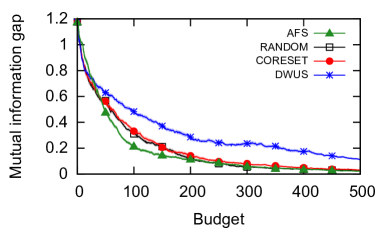
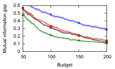
Figure 4: AFS vs baseline: BASEHOCK, $k=20$. Top: full experiment. Bottom: Zoom in.

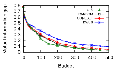
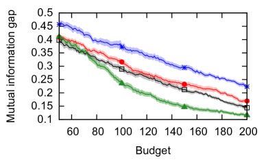
Figure 5: AFS vs baseline: PCMAC, $k=20$. Top: full experiment. Bottom: Zoom in.

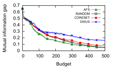
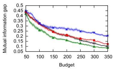
Figure 6: AFS vs baseline: RELATHE, $k=20$. Top: full experiment. Bottom: Zoom in.

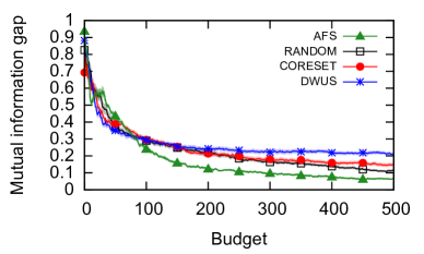
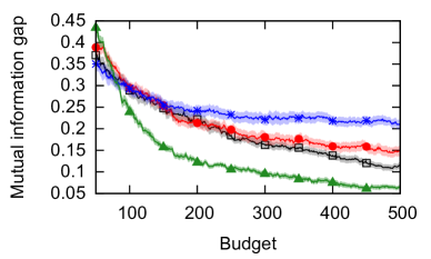
Figure 7: AFS vs baseline: MUSK, $k=20$. Top: full experiment. Bottom: Zoom in.

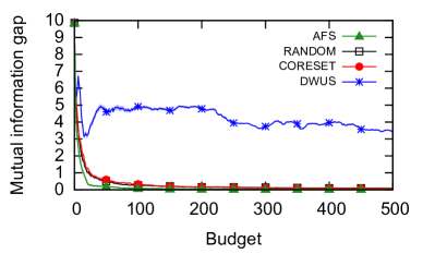
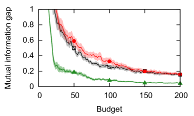
Figure 8: AFS vs baseline: MNIST: 0 vs 1, $k=20$. Top: full experiment. Bottom: Zoom in.

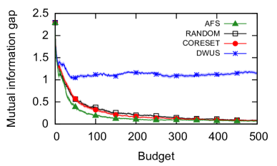
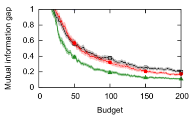
Figure 9: AFS vs baseline: MNIST: 3 vs 5, $k=20$. Top: full experiment. Bottom: Zoom in.

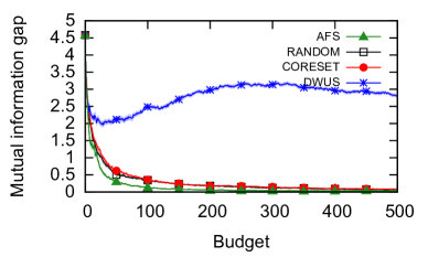
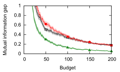
Figure 10: AFS vs baseline: MNIST: 4 vs 6, $k=20$. Top: full experiment. Bottom: Zoom in.

B.2 Comparing to baselines: $k=10$

The first set of graphs shows the experiments for $k=10$.

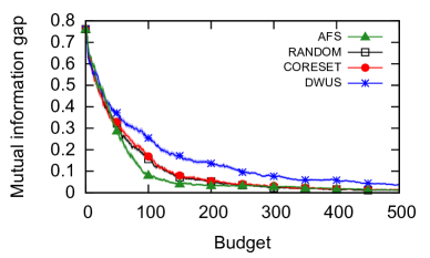
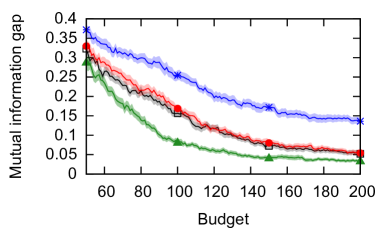
Figure 11: AFS vs baseline: BASEHOCK, $k=10$. Top: full experiment. Bottom: Zoom in.

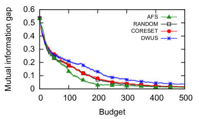
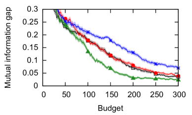
Figure 12: AFS vs baseline: PCMAC, $k=10$. Top: full experiment. Bottom: Zoom in.

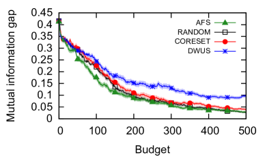
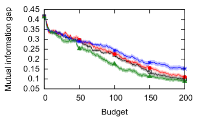
Figure 13: AFS vs baseline: RELATHE, $k=10$. Top: full experiment. Bottom: Zoom in.

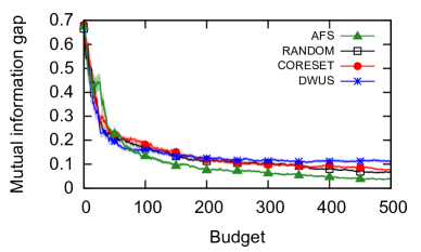
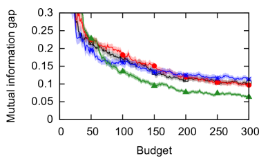
Figure 14: AFS vs baseline: MUSK, $k=10$. Top: full experiment. Bottom: Zoom in.

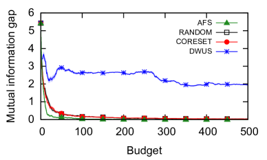
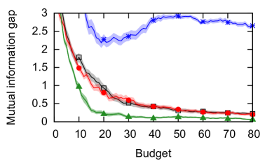
Figure 15: AFS vs baseline: MNIST: 0 vs 1, $k=10$. Top: full experiment. Bottom: Zoom in.

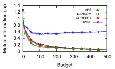
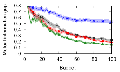
Figure 16: AFS vs baseline: MNIST: 3 vs 5, $k=10$. Top: full experiment. Bottom: Zoom in.

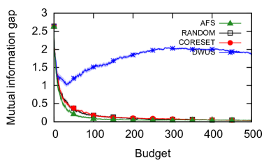
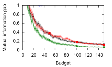
Figure 17: AFS vs baseline: MNIST: 4 vs 6, $k=10$. Top: full experiment. Bottom: Zoom in.

B.3 Comparing to baselines: $k=5$

The next set of graphs shows the experiments for $k=5$. Here too, AFS performs the best compared to the other baselines, although the difference is less pronounced, possibly due to the smaller value of $k$.

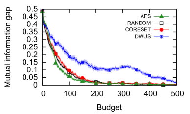
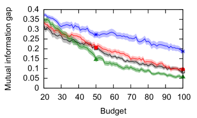
Figure 18: AFS vs baseline: BASEHOCK, $k=5$. Top: full experiment. Bottom: Zoom in.

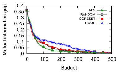
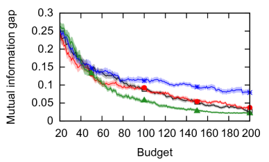
Figure 19: AFS vs baseline: PCMAC, $k=5$. Top: full experiment. Bottom: Zoom in.

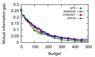
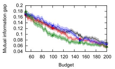
Figure 20: AFS vs baseline: RELATHE, $k=5$. Top: full experiment. Bottom: Zoom in.

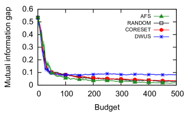
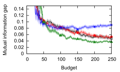
Figure 21: AFS vs baseline: MUSK, $k=5$. Top: full experiment. Bottom: Zoom in.

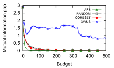
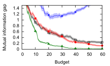
Figure 22: AFS vs baseline: MNIST: 0 vs 1, $k=5$. Top: full experiment. Bottom: Zoom in.

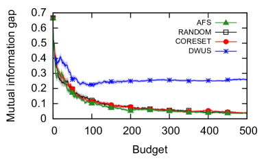
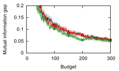
Figure 23: AFS vs baseline: MNIST: 3 vs 5, $k=5$. Top: full experiment. Bottom: Zoom in.

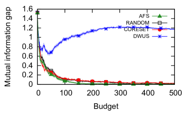
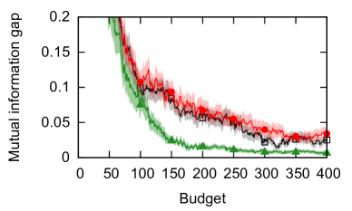
Figure 24: AFS vs baseline: MNIST: 4 vs 6, $k=5$. Top: full experiment. Bottom: Zoom in.

B.4 Comparing to baselines: $k=1$

The last set of graphs shows the experiments comparing AFS to the baseline for $k=1$. For $k=1$, AFS performs comparably with CORESET and RANDOM. However, the DWUS baseline performs significantly worse in many of the experiments.

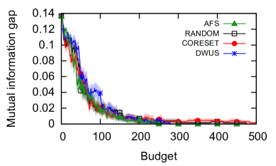
Figure 25: AFS vs baseline: BASEHOCK, $k=1$.

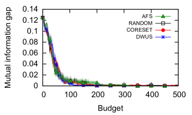
Figure 26: AFS vs baseline: PCMAC, $k=1$.

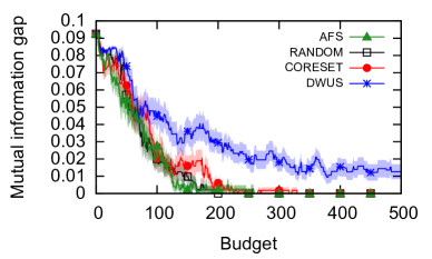
Figure 27: AFS vs baseline: RELATHE, $k=1$.

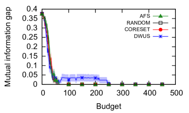
Figure 28: AFS vs baseline: MUSK, $k=1$.

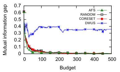
Figure 29: AFS vs baseline: MNIST: 0 vs 1, $k=1$.

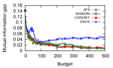
Figure 30: AFS vs baseline: MNIST: 3 vs 5, $k=1$.

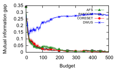
Figure 31: AFS vs baseline: MNIST: 4 vs 6, $k=1$.

Appendix C Experiments: Ablation tests

The following graphs show the results of the ablation experiments. The $x$ axis is the label budget, and the $y$ axis is the mutual information gap, calculated via $\sum_{j\in F^{*}}H_{j}-\sum_{j\in F}H_{j}$, as explained in Section 6. Each graph averages $30$ runs with budgets up to $500$ queries. The shaded areas provide the 95% confidence intervals. For each experiment, we show the full graph at the top and a zoomed-in version at the bottom, which allows better visibility of the interesting parts of the graph.

AVG-SEL, which avoids the bias-correction term, performs quite poorly in many of the cases. SINGLE, which uses a single feature for scoring, is also usually worse than AFS. AVG-ALL, which averages the score over all the features, is inconsistent and sometimes performs very poorly, although it sometimes performs better than the other options.

Lastly, AFS-NOSG, which has no safeguard in case the estimates converge to a wrong value, usually performs similarly to AFS, but in some cases (most significantly, the RELATHE data set, Figure 41 and Figure 48) it is significantly worse even compared to the random baseline. It also sometimes performs better than AFS. Nonetheless, AFS-NOSG is overall less robust due to its failure to converge to a low gap in some cases. These results show that the full AFS algorithm performs well the most consistently.

C.1 Ablation tests: $k=20$

The following graphs gives the results of the ablation tests for $k=20$.

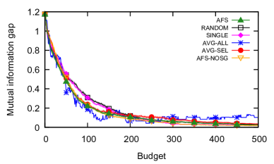
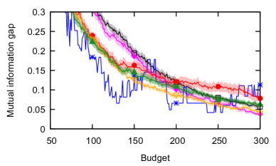
Figure 32: Ablation tests: BASEHOCK ($k=20$). Top: full experiment. Bottom: Zoom in.

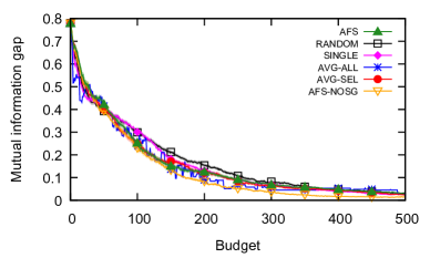
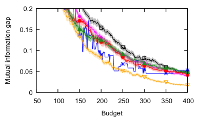
Figure 33: Ablation tests: PCMAC ($k=20$). Top: full experiment. Bottom: Zoom in.

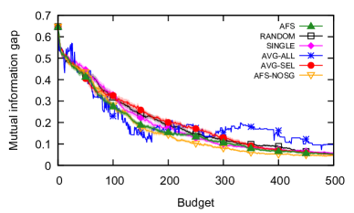
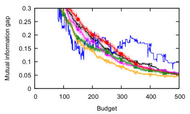
Figure 34: Ablation tests: RELATHE ($k=20$). Top: full experiment. Bottom: Zoom in.

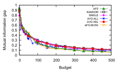
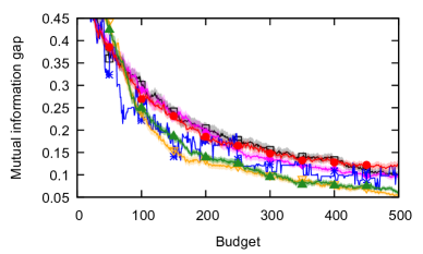
Figure 35: Ablation tests: MUSK ($k=20$). Top: full experiment. Bottom: Zoom in.

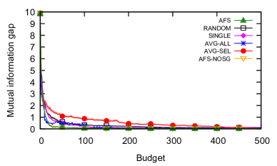
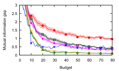
Figure 36: Ablation tests: MNIST: 0 vs 1 ($k=20$). Top: full experiment. Bottom: Zoom in.

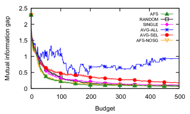
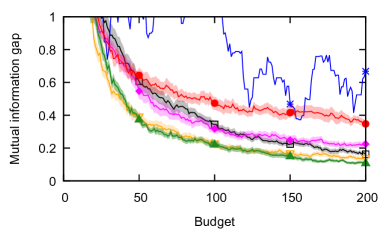
Figure 37: Ablation tests: MNIST: 3 vs 5 ($k=20$). Top: full experiment. Bottom: Zoom in.

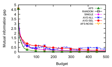
Figure 38: Ablation tests: MNIST: 4 vs 6 ($k=20$). Top: full experiment. Bottom: Zoom in.

C.2 Ablation tests: $k=10$

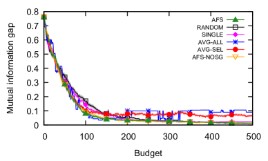
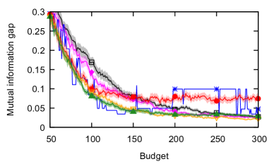
Figure 39: Ablation tests: BASEHOCK ($k=10$). Top: full experiment. Bottom: Zoom in.

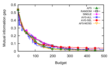
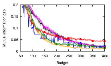
Figure 40: Ablation tests: PCMAC ($k=10$). Top: full experiment. Bottom: Zoom in.

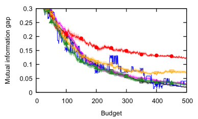
Figure 41: Ablation tests: RELATHE ($k=10$). Top: full experiment. Bottom: Zoom in. Here, AFS-NOSG is significantly worse than AFS and does not converge to a low gap.

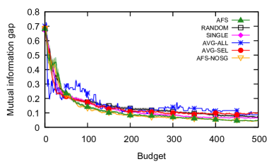
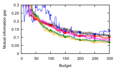
Figure 42: Ablation tests: MUSK ($k=10$). Top: full experiment. Bottom: Zoom in.

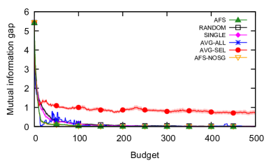
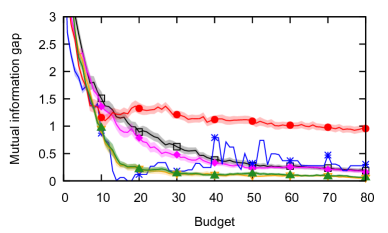
Figure 43: Ablation tests: MNIST: 0 vs 1 ($k=10$). Top: full experiment. Bottom: Zoom in.

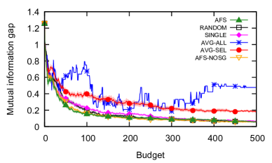
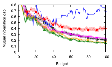
Figure 44: Ablation tests: MNIST: 3 vs 5 ($k=10$). Top: full experiment. Bottom: Zoom in.

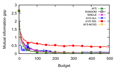
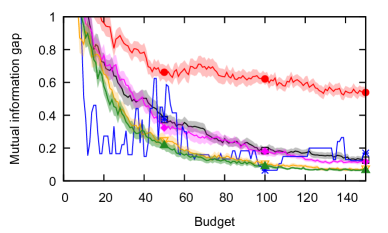
Figure 45: Ablation tests: MNIST: 4 vs 6 ($k=10$). Top: full experiment. Bottom: Zoom in.

C.3 Ablation tests: $k=5$

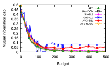
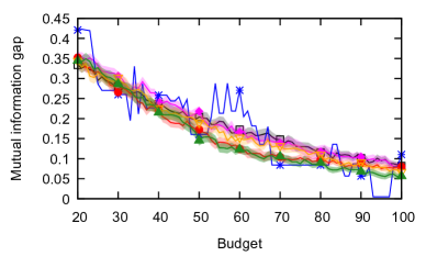
Figure 46: Ablation tests: BASEHOCK ($k=5$). Top: full experiment. Bottom: Zoom in.

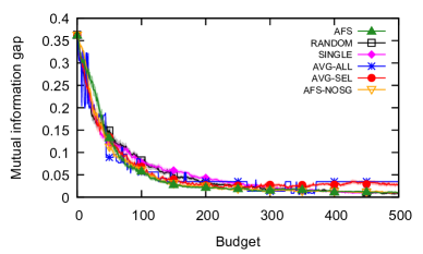
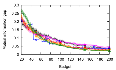
Figure 47: Ablation tests: PCMAC ($k=5$). Top: full experiment. Bottom: Zoom in.

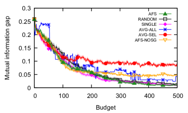
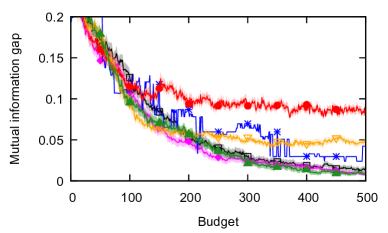
Figure 48: Ablation tests: RELATHE ($k=5$). Top: full experiment. Bottom: Zoom in. Here, AFS-NOSG is significantly worse than AFS and does not converge to a low gap.

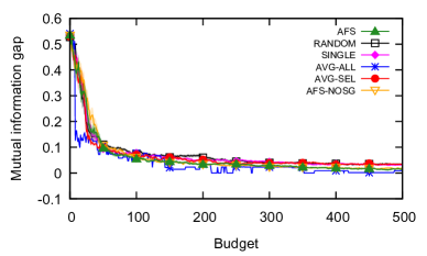
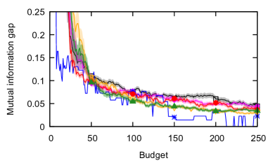
Figure 49: Ablation tests: MUSK ($k=5$). Top: full experiment. Bottom: Zoom in.

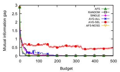
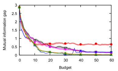
Figure 50: Ablation tests: MNIST: 0 vs 1 ($k=5$). Top: full experiment. Bottom: Zoom in.

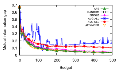
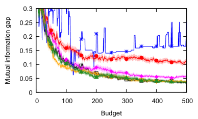
Figure 51: Ablation tests: MNIST: 3 vs 5 ($k=5$). Top: full experiment. Bottom: Zoom in.

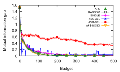
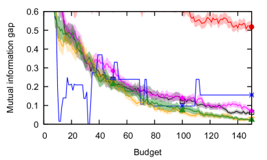
Figure 52: Ablation tests: MNIST: 4 vs 6 ($k=5$). Top: full experiment. Bottom: Zoom in.

Appendix D Experiments: Comparing aggregation functions

We report experiments comparing possible choices of the aggregation function $\psi$. We tested the $\ell_{1},\ell_{\infty}$ and $\ell_{2}$ norms. It can be seen that the results are similar for $\ell_{1}$ and $\ell_{2}$, while $\ell_{\infty}$ is sometimes slightly worse. Thus, while we chose $\ell_{1}$, setting $\psi\mathrel{\mathop{\ordinarycolon}}=\ell_{2}$ is also a valid choice. For easy comparison, the graphs show the RANDOM baseline as well.

D.1 Comparing aggregation functions: $k=20$

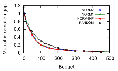
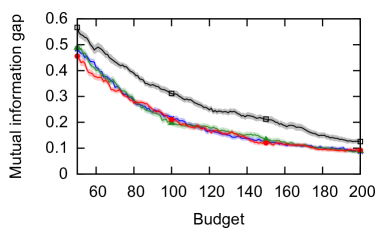
Figure 53: Choices of $\psi$: BASEHOCK ($k=20$). Top: full experiment. Bottom: Zoom in.

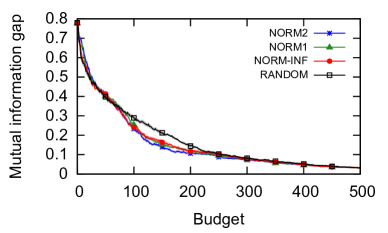
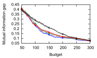
Figure 54: Choices of $\psi$: PCMAC ($k=20$). Top: full experiment. Bottom: Zoom in.

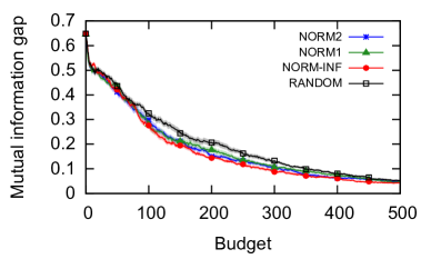
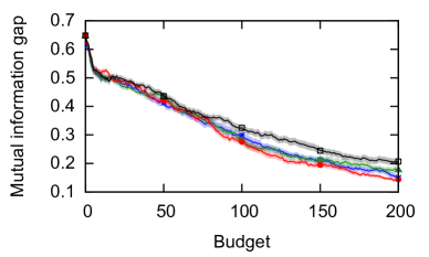
Figure 55: Choices of $\psi$: RELATHE ($k=20$). Top: full experiment. Bottom: Zoom in.

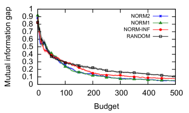
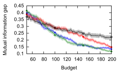
Figure 56: Choices of $\psi$: MUSK ($k=20$). Top: full experiment. Bottom: Zoom in.

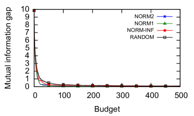
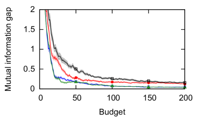
Figure 57: Choices of $\psi$: MNIST: 0 vs 1 ($k=20$). Top: full experiment. Bottom: Zoom in.

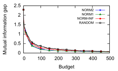
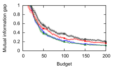
Figure 58: Choices of $\psi$: MNIST: 3 vs 5 ($k=20$). Top: full experiment. Bottom: Zoom in.

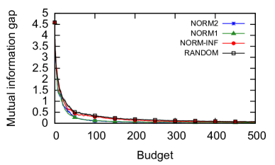
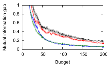
Figure 59: Choices of $\psi$: MNIST: 4 vs 6 ($k=20$). Top: full experiment. Bottom: Zoom in.

D.2 Comparing aggregation functions: $k=10$

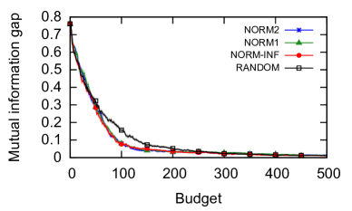
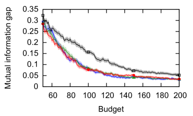
Figure 60: Choices of $\psi$: BASEHOCK ($k=10$). Top: full experiment. Bottom: Zoom in.

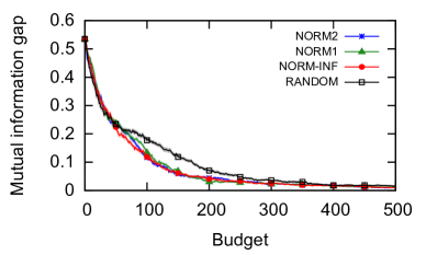
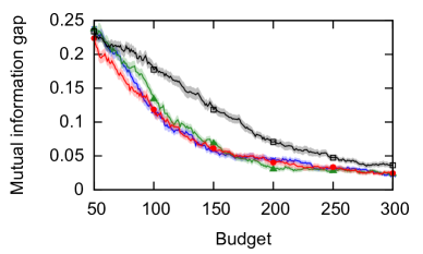
Figure 61: Choices of $\psi$: PCMAC ($k=10$). Top: full experiment. Bottom: Zoom in.

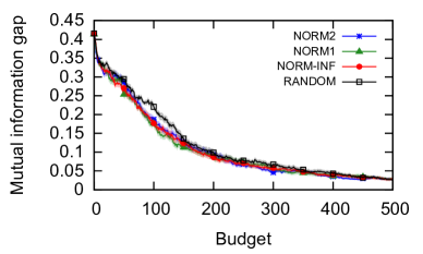
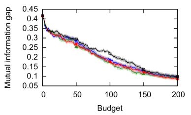
Figure 62: Choices of $\psi$: RELATHE ($k=10$). Top: full experiment. Bottom: Zoom in.

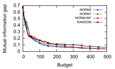
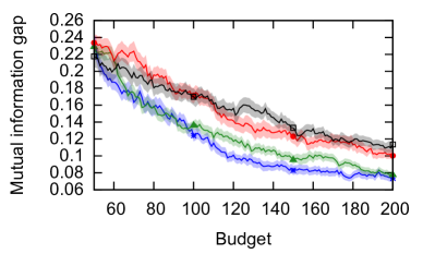
Figure 63: Choices of $\psi$: MUSK ($k=10$). Top: full experiment. Bottom: Zoom in.

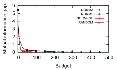
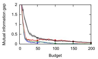
Figure 64: Choices of $\psi$: MNIST: 0 vs 1 ($k=10$). Top: full experiment. Bottom: Zoom in.

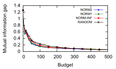
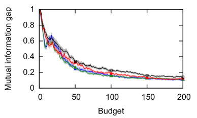
Figure 65: Choices of $\psi$: MNIST: 3 vs 5 ($k=10$). Top: full experiment. Bottom: Zoom in.

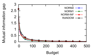
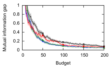
Figure 66: Choices of $\psi$: MNIST: 4 vs 6 ($k=10$). Top: full experiment. Bottom: Zoom in.

D.3 Comparing aggregation functions: $k=5$

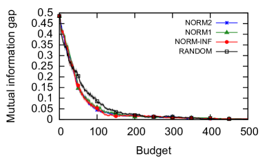
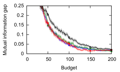
Figure 67: Choices of $\psi$: BASEHOCK ($k=5$). Top: full experiment. Bottom: Zoom in.

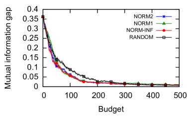
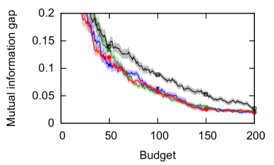
Figure 68: Choices of $\psi$: PCMAC ($k=5$). Top: full experiment. Bottom: Zoom in.

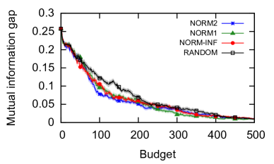
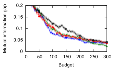
Figure 69: Choices of $\psi$: RELATHE ($k=5$). Top: full experiment. Bottom: Zoom in.

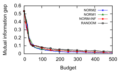
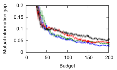
Figure 70: Choices of $\psi$: MUSK ($k=5$). Top: full experiment. Bottom: Zoom in.

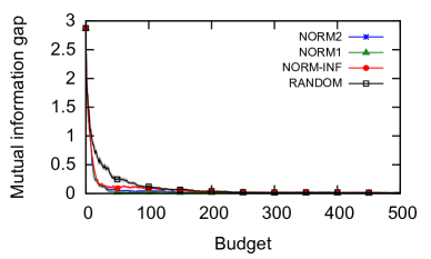
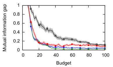
Figure 71: Choices of $\psi$: MNIST: 0 vs 1 ($k=5$). Top: full experiment. Bottom: Zoom in.

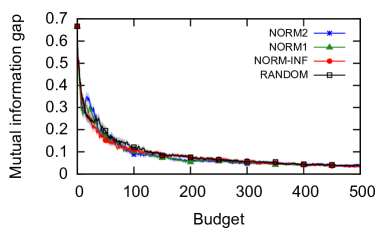
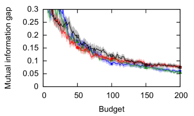
Figure 72: Choices of $\psi$: MNIST: 3 vs 5 ($k=5$). Top: full experiment. Bottom: Zoom in.

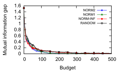
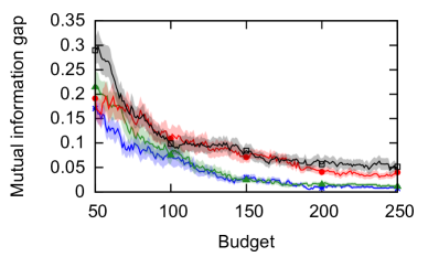
Figure 73: Choices of $\psi$: MNIST: 4 vs 6 ($k=5$). Top: full experiment. Bottom: Zoom in.

D.4 Comparing aggregation functions: $k=1$

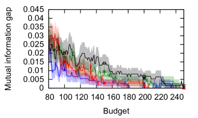
Figure 74: Choices of $\psi$: BASEHOCK ($k=1$). Top: full experiment. Bottom: Zoom in.

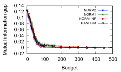
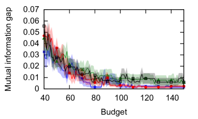
Figure 75: Choices of $\psi$: PCMAC ($k=1$). Top: full experiment. Bottom: Zoom in.

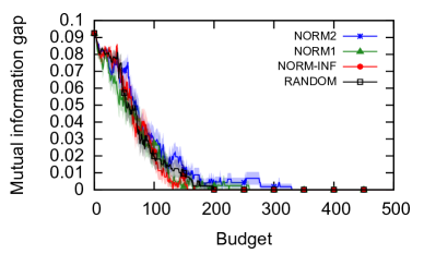
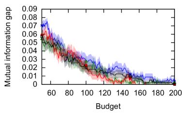
Figure 76: Choices of $\psi$: RELATHE ($k=1$). Top: full experiment. Bottom: Zoom in.

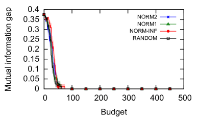
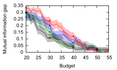
Figure 77: Choices of $\psi$: MUSK ($k=1$). Top: full experiment. Bottom: Zoom in.

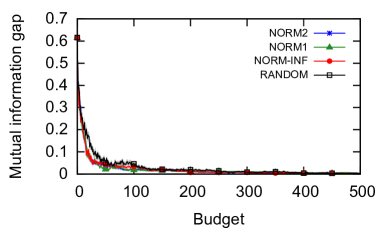
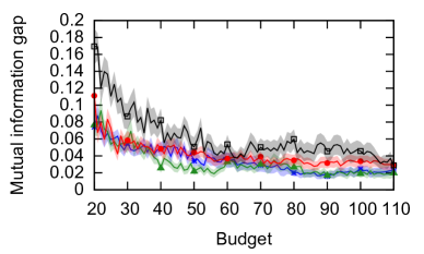
Figure 78: Choices of $\psi$: MNIST: 0 vs 1 ($k=1$). Top: full experiment. Bottom: Zoom in.

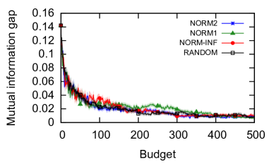
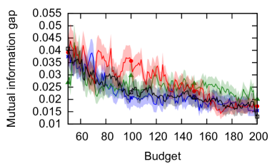
Figure 79: Choices of $\psi$: MNIST: 3 vs 5 ($k=1$). Top: full experiment. Bottom: Zoom in.

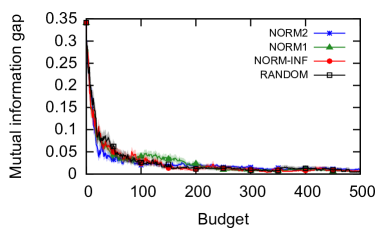
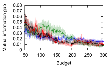
Figure 80: Choices of $\psi$: MNIST: 4 vs 6 ($k=1$). Top: full experiment. Bottom: Zoom in.

References

- Amaldi and Kann (1998) Amaldi, E.; and Kann, V. 1998. On the approximability of minimizing nonzero variables or unsatisfied relations in linear systems. Theoretical Computer Science 209(1-2): 237–260.
- Antos, Grover, and Szepesvári (2008) Antos, A.; Grover, V.; and Szepesvári, C. 2008. Active learning in multi-armed bandits. In International Conference on Algorithmic Learning Theory, 287–302. Springer.
- Benaroya, Han, and Nagurka (2005) Benaroya, H.; Han, S. M.; and Nagurka, M. 2005. Probability models in engineering and science. CRC press.
- Bernstein (1924) Bernstein, S. N. 1924. On a modification of Chebyshev’s inequality and of the error formula of Laplace. Annals Science Institute Sav. Ukraine Sect. Math. 1.
- Carpentier et al. (2011) Carpentier, A.; Lazaric, A.; Ghavamzadeh, M.; Munos, R.; and Auer, P. 2011. Upper-confidence-bound algorithms for active learning in multi-armed bandits. In International Conference on Algorithmic Learning Theory, 189–203. Springer.
- Chen et al. (2014) Chen, S.; Lin, T.; King, I.; Lyu, M. R.; and Chen, W. 2014. Combinatorial pure exploration of multi-armed bandits. In Advances in Neural Information Processing Systems, 379–387.
- Clopper and Pearson (1934) Clopper, C. J.; and Pearson, E. S. 1934. The use of confidence or fiducial limits illustrated in the case of the binomial. Biometrika 26(4): 404–413.
- Cohn, Atlas, and Ladner (1994) Cohn, D.; Atlas, L.; and Ladner, R. 1994. Improving generalization with active learning. Machine Learning 15: 201–221.
- Dua and Graff (2019) Dua, D.; and Graff, C. 2019. UCI Machine Learning Repository. URL http://archive.ics.uci.edu/ml.
- Garivier and Kaufmann (2016) Garivier, A.; and Kaufmann, E. 2016. Optimal best arm identification with fixed confidence. In Conference on Learning Theory, 998–1027.
- Guyon et al. (2008) Guyon, I.; Gunn, S.; Nikravesh, M.; and Zadeh, L. A. 2008. Feature extraction: foundations and applications, volume 207. Springer.
- Hastie, Tibshirani, and Friedman (2001) Hastie, T.; Tibshirani, R.; and Friedman, J. 2001. The Elements of Statistical Learning. Springer.
- Hoeffding (1963) Hoeffding, W. 1963. Probability inequalities for sums of bounded random variables. Journal of the American Statistical Association 58(301): 13–30.
- Kalyanakrishnan and Stone (2010) Kalyanakrishnan, S.; and Stone, P. 2010. Efficient Selection of Multiple Bandit Arms: Theory and Practice. In ICML, volume 10, 511–518.
- Kira and Rendell (1992) Kira, K.; and Rendell, L. A. 1992. The feature selection problem: Traditional methods and a new algorithm. In Aaai, volume 2, 129–134.
- LeCun and Cortes (2010) LeCun, Y.; and Cortes, C. 2010. MNIST handwritten digit database. http://yann.lecun.com/exdb/mnist/. URL http://yann.lecun.com/exdb/mnist/.
- Li et al. (2018) Li, J.; Cheng, K.; Wang, S.; Morstatter, F.; Trevino, R. P.; Tang, J.; and Liu, H. 2018. Feature selection: A data perspective. ACM Computing Surveys (CSUR) 50(6): 94. URL –http://featureselection.asu.edu˝.
- Liu, Motoda, and Yu (2004) Liu, H.; Motoda, H.; and Yu, L. 2004. A selective sampling approach to active feature selection. Artificial Intelligence 159(1-2): 49–74.
- Liu et al. (2003) Liu, H.; Yu, L.; Dash, M.; and Motoda, H. 2003. Active feature selection using classes. In Pacific-Asia Conference on Knowledge Discovery and Data Mining, 474–485. Springer.
- McCallum and Nigam (1998) McCallum, A. K.; and Nigam, K. 1998. Employing EM and pool-based active learning for text classification. In Proc. International Conference on Machine Learning (ICML), 359–367. Citeseer.
- Nguyen and Smeulders (2004) Nguyen, H. T.; and Smeulders, A. 2004. Active learning using pre-clustering. In Proceedings of the twenty-first international conference on Machine learning, 79.
- Paninski (2003) Paninski, L. 2003. Estimation of entropy and mutual information. Neural computation 15: 1191–1253.
- Ros and Guillaume (2017) Ros, F.; and Guillaume, S. 2017. DIDES: a fast and effective sampling for clustering algorithm. Knowledge and information systems 50(2): 543–568.
- Ros and Guillaume (2020) Ros, F.; and Guillaume, S. 2020. Sampling Techniques for Supervised Or Unsupervised Tasks. Springer.
- Sabato and Shalev-Shwartz (2008) Sabato, S.; and Shalev-Shwartz, S. 2008. Ranking Categorical Features Using Generalization Properties. Journal of Machine Learning Research 9: 1083–1114.
- Yang et al. (2017) Yang, Y.-Y.; Lee, S.-C.; Chung, Y.-A.; Wu, T.-E.; Chen, S.-A.; and Lin, H.-T. 2017. libact: Pool-based Active Learning in Python. Technical report, National Taiwan University. URL https://github.com/ntucllab/libact. Available as arXiv preprint https://arxiv.org/abs/1710.00379.
- Zhang (2018) Zhang, C. 2018. Efficient active learning of sparse halfspaces. arXiv preprint arXiv:1805.02350 .