Largest similar copies of convex polygons amidst polygonal obstacles

Abstract

Given a convex polygon $P$ with $k$ vertices and a polygonal domain $Q$ consisting of polygonal obstacles with total size $n$ in the plane, we study the optimization problem of finding a largest similar copy of $P$ that can be placed in $Q$ without intersecting the obstacles. We improve the time complexity for solving the problem to $O(k^{2}n^{2}\lambda_{4}(k)\log{n})$. This is progress of improving the previously best known results by Chew and Kedem [SoCG89, CGTA93] and Sharir and Toledo [SoCG91, CGTA94] on the problem in more than 25 years.

1 Introduction

Finding a largest object of a certain shape that can be placed in a polygonal environment has been considered as a fundamental problem in computational geometry. This kind of optimization problem arises in various applications, including the metal industry where we want to find a largest similar pattern containing no faults in a piece of material. There is also a correspondence to motion planning problems [18, 14, 12] and shape matching [10].

Polygon placement. In the polygon containment problem, we are given a container and a fixed shape, and want to find a largest object of the shape that can be inscribed in the container. There are various assumptions on the object to be placed, the motions allowed, and the environment the object is to be placed within. In many cases, the container is a convex or simple polygon, possibly with holes. Typical shapes are squares, triangles with fixed interior angles, and rectangles with fixed aspect ratios. For the motions, we may allow translation or both translation and rotation, together with scaling. When scaling is not allowed, the problem is to find a copy of a given object under translation or rigid motion that can be inscribed in a polygon [6, 4]. When both translation and scaling are allowed, the objective becomes to find a largest homothetic copy of a given object that can be inscribed in a polygonal domain [11, 16]. When rotation is allowed, together with translation and scaling, the problem is to find a largest similar copy of a given object and it becomes more involved; it may require to capture every change induced by the rotation to the underlying structure maintained by the algorithms, and therefore the complexity of the algorithms may depend on the changes during the rotation.

In this paper, we consider the polygon containment problem under translation, rotation, and scaling. We aim to find a largest similar copy of a given convex polygon $P$ with $k$ vertices that can be inscribed in a polygonal domain $Q$ consisting of $n$ points and line segments. This problem has been considered fairly well in computational geometry community for many years. See Chapter 50 of the Handbook of Discrete and Computational Geometry [12].

The earliest result was perhaps the SoCG’89 paper by Chew and Kedem [7]. They considered the problem and gave an incremental technique for handling all the combinatorial changes to the Delaunay triangulation of the polygonal domain $Q$ under the distance function induced by the input polygon $P$ while $P$ is rotating. They gave an upper bound $O(k^{4}n\lambda_{4}(kn))$ on the combinatorial changes, that is, the number of critical orientations, together with a deterministic $O(k^{4}n\lambda_{4}(kn)\log{n})$-time algorithm, where $\lambda_{s}(n)$ the length of the longest Davenport–Schinzel sequence of order $s$ including $n$ distinct symbols. A few years later, the bound was improved to $O(k^{4}n\lambda_{3}(n))$ by them, and thus the running time of the algorithm became $O(k^{4}n\lambda_{3}(n)\log{n})$ [8].

Toledo [21], and Sharir and Toledo [19] studied this problem (they called this problem the extremal polygon containment problem) and applied the motion-planning algorithm [14] to solve this problem. They gave an algorithm with running time $O(k^{2}n\lambda_{4}(kn)\log^{3}(kn)\allowbreak\log\log(kn))$ that uses the parametric search technique of Megiddo [17].

These two results, $O(k^{4}n\lambda_{3}(n)\log{n})$ and $O(k^{2}n\lambda_{4}(kn)\log^{3}(kn)\allowbreak\log\log(kn))$, are comparable to each other. The latter one implies a better time bound for large $k$ ($k>n$) while the former one implies a better time bound for small $k$.

There was a randomized algorithm by Agarwal et al. [2] that finds a largest similar copy in $O(kn\lambda_{6}(kn)\log^{3}(kn)\log^{2}{n})$ expected time using parametric search technique of Megiddo [17]. The problem was also considered for special cases. Agarwal et al. [1] considered the problem of finding largest similar copy of a given convex $k$-gon with contained in a convex $n$-gon and gave an $O(kn^{2}\log{n})$-time algorithm. Very recently, there were results on two variants. Bae and Yoon [5] gave an $O(n^{2}\log{n})$-time algorithm for finding a largest empty square among a set of $n$ points in the plane. Lee et al. [15] gave an algorithm for finding a largest triangle with fixed interior angles in a simple polygon with $n$ vertices in $O(n^{2}\log{n})$ time.

However, no improvement to the worst-case time bounds by Chew and Kedem, and Sharir and Toledo has been known for the polygon placement problem.

New result. We make progress of improving the upper bound on the combinatorial changes considered during the rotation and the algorithm to compute a largest similar copy. We present an upper bound $O(k^{2}n^{2}\lambda_{4}(k))$ on the combinatorial changes, and this directly improves the time bound for the algorithm to $O(k^{2}n^{2}\lambda_{4}(k)\log{n})$. This improves the previously best known results by Chew and Kedem [8] and Sharir and Toledo [19] in more than 25 years.

Compared to the combinatorial upper bound $O(k^{4}n\lambda_{3}(n))$ by Chew and Kedem, our bound is smaller than their bound asymptotically for both $k$ and $n$. Since $\lambda_{4}(k)=o(k\log^{*}k)$ [20] and $\lambda_{3}(n)=\Theta(n\alpha(n))$, our bound is $o(k^{3}n^{2}\log^{*}k)$ while their bound is $O(k^{4}n^{2}\alpha(n))$. Therefore, our algorithm outperforms theirs. Compared to the time bound $O(k^{2}n\lambda_{4}(kn)\log^{3}(kn)\allowbreak\log\log(kn))$ by Sharir and Toledo [19], our running time outperforms theirs for both $k$ and $n$ without resorting to parametric search technique, because $n\lambda_{4}(k)\log n=o(\lambda_{4}(kn)\log^{3}(kn)\allowbreak\log\log(kn))$.

Thus our result improves the best result for the problem introduced in Chapter 50 of the Handbook of Discrete and Computational Geometry [12], and the result could be a stepping stone to closing the problem.

Overview of techniques. We achieve the improved upper bound by carefully analyzing the combinatorial changes in the edge Delaunay triangulation of $Q$ (to be defined later, shortly eDT) while rotating $P$ and by reducing the candidate size to consider for the changes. Following the approach of Chew and Kedem [8], our strategy consists of two parts: Counting the combinatorial changes in eDT for a constant $k$, and then counting the combinatorial changes with respect to $k$.

1. In the first part, we analyze the combinatorial changes for a fixed $k$. We consider a family of functions defined for each vertex and edge of $P$ and compute their lower envelope. Since there are $O(k)$ vertices and edges of $P$, we compute $O(k)$ lower envelopes. We show that the complexity of each lower envelope is $O(n)$. Then we compute the breakpoints on the lower envelope of the $O(k)$ lower envelopes. To bound the number of combinatorial changes in eDT, we consider a placement of a scaled copy of $P$ such that a vertex of $Q$ and a vertex of $P$ are in contact, which we call a hinge, and show that the number of breakpoints on the lower envelope defined for each hinge is $O(n)$. Since there are $O(n)$ hinges for a constant $k$, the number of combinatorial changes in eDT for $\theta$ increasing from 0 to $2\pi$ is $O(n^{2})$.

2. In the second part, we analyze the combinatorial changes to eDT with respect to $k$. A combinatorial change to eDT corresponds to a quadruplet of pairs, each pair consisting of an element of $Q$ and an element of $P$ touching each other in some placement of a scaled copy of $P$ simultaneously. To count the quadruplets inducing combinatorial changes to eDT, we consider the triplets of such pairs and define a function for each triplet implying the size of the scaled copy of $P$ defined by the triplet, satisfying the followings: For the lower envelope $L$ of the functions, a combinatorial change corresponds to an intersection of two such functions appearing on $L$. That is, every combinatorial change to eDT occurs at a breakpoint on the lower envelope of the functions. So, the complexity of the lower envelope bounds the number of combinatorial changes that occur during the rotation of $P$. We reduce the complexity bound on the lower envelope by classifying the combination of pairs for the quadruplets.

While this high-level strategy may appear similar to the previous one [8], there are a few major differences and difficulties in improving the bound. In the first part, we improve the previous bound $O(n\lambda_{3}(n))$ by Chew and Kedem as follows. We partition the family of functions to subfamilies such that the functions in the same subfamily have the same domain length, and therefore the complexity of their lower envelope becomes linear to the number of functions [5, 15]. Thus, the total upper bound is improved to $O(n^{2})$.

In the second part, instead of the quadruplets considered by Chew and Kedem, we consider the triplets of pairs only and show that the functions for the triplets, in their lower envelope, give us an upper bound on the number of the combinatorial changes to eDT. These functions must reflect the placement of a scaled copy of $P$ that can be inscribed in $Q$ as well as the scaling factor. We present a function definition satisfying this requirement and show that every combinatorial change to eDT occurs at a breakpoint on the lower envelope of the functions. There are $O(k^{3}n^{2})$ such functions and two functions intersect at most four times. Thus, the complexity of the lower envelope of the functions is $O(\lambda_{6}(k^{3}n^{2}))$ as the lower envelope corresponds to a Davenport-Schinzel sequence of order 6. To reduce the bound, we classify the functions into types based on the combinations of pairs defining the functions and show that any two functions belonging to the same type intersect each other less than four times. By applying the partition method in the first part and the classification above on the functions, we show that the complexity of the lower envelope becomes $O(k^{2}n^{2}\lambda_{4}(k))$.

Due to the limit of space, the proofs of some lemmas and corollaries are given in Appendix.

2 Preliminary

2.1 Davenport–Schinzel sequences and lower envelopes

A Davenport–Schinzel sequence is a sequence of symbols in which the frequency of any two symbols appearing in alternation is limited. We call a Davenport–Schinzel sequence of order $s$ that includes $n$ distinct symbols a $\mathrm{DS}(n,s)$-sequence, and denote by $\lambda_{s}(n)$ the length of the longest $\mathrm{DS}(n,s)$-sequence. For a $\mathrm{DS}(n,s)$-sequence $U$, let $U(j)$ denote the $j$-th entry of $U$. We say a symbol $a_{i}$ of $U$ is active at $j$ if $U(j^{\prime})=a_{i}$ and $U(j^{\prime\prime})=a_{i}$ for some $j^{\prime}\leq j$ and $j^{\prime\prime}>j$. Let $\nu(j)$ denote the number of active symbols of $U$ at $j$. We say $U$ is a $\mathrm{DS}(n,s,m)$-sequence if $\nu(j)\leq m$ for each $j$. We denote by $\lambda_{s,m}(n)$ the length of the longest $\mathrm{DS}(n,s,m)$-sequence.

We use some properties and lemmas related to Davenport–Schinzel sequences in analyzing algorithms. Let $\mathcal{F}=\{f_{1},\dots,f_{n}\}$ be a collection of $n$ partially-defined, continuous, one-variable real-valued functions. The points at which two functions intersect in their graphs and endpoints of function graphs are called the breakpoints. If any two functions $f_{i}$ and $f_{j}$ intersect in their graphs at most $s$ times, the lower envelope of $\mathcal{F}$ has at most $\lambda_{s+2}(n)$ breakpoints [3]. We introduce some technical lemmas that are used in Section 3.

Lemma 1 (Lemma 14 of [15]).

Assume any two functions $f_{i}$ and $f_{j}$ intersect in their graphs at most once and each function $f_{i}$ has domain $D_{i}$ of length $d$. If there is a constant $c$ such that $|{\bigcup}{D_{i}}|=cd$, then the lower envelope of $\mathcal{F}$ has $O(n)$ breakpoints.

Proof.

Let $D_{\mathcal{F}}$ be the union of all ${D_{i}}$’s. Let $l_{i}$ be the point of $D_{\mathcal{F}}$ at distance $di$ from the leftmost point of $D_{\mathcal{F}}$, for $i=0,1,\ldots,\lceil c\rceil$. Then $l_{j}<l_{j^{\prime}}$ for any two indices $0\leq j<j^{\prime}\leq\lceil c\rceil$. Then these points $l_{i}$’s partition $D_{\mathcal{F}}$ into intervals such that each interval has length $d$, except the last one of length smaller than or equal to $d$. Observe that each $D_{i}$ intersects at most two consecutive intervals.

Let $L(j)=\{f_{i}|_{[l_{j-1},l_{j}]}\mid l_{j}\in{D_{i}}\}$ and $R(j)=\{f_{i}|_{[l_{j},l_{j+1}]}\mid l_{j}\in{D_{i}}\}$ be the sets of functions defined on the intervals with $0<j<\lceil c\rceil$. Since any two functions in $L(j)$ intersect in their graphs at most once and their domains have $l_{j}$ as the right endpoint, the lower envelope of $L(j)$ forms a Davenport–Schinzel sequence of order 2, and therefore the lower envelope of $L(j)$ has complexity $O(|L(j)|)$. Similarly, the lower envelope of $R(j)$ has complexity $O(|R(j)|)$. Since the union $U_{L}$ of all $L(j)$’s and the union $U_{R}$ of all $R(j)$’s have $O(n)$ functions, the lower envelope of each union has complexity $O(n)$.

Now, consider a new partition of $D_{\mathcal{F}}$ obtained by slicing it at every breakpoint on the lower envelopes of $U_{L}$ and $U_{R}$. Since there are $O(n)$ such breakpoints and the lower envelope of $\mathcal{F}$ restricted to a component of the new partition has a constant complexity, the complexity of the lower envelope of $\mathcal{F}$ is $O(n)$. ∎

Lemma 2 (Lemma 1 of [13]).

$\lambda_{s,m}(n)$ is $O(\frac{n}{m}\lambda_{s}(m))$.

Corollary 3.

Let $\mathcal{G}=\{g_{1},\dots,g_{m}\}$ be a collection of $m$ partially-defined, piecewise continuous, one-variable real-valued functions. Let $n$ be the total number of continuous pieces in the function graphs of $\mathcal{G}$. If any pair of continuous pieces intersect in at most $s$ points, the lower envelope of $\mathcal{G}$ has $O(\frac{n}{m}\lambda_{s+2}(m))$ breakpoints.

Proof.

Let $\mathcal{G^{\prime}}=\{g^{\prime}_{1},\dots,g^{\prime}_{n}\}$ be the set of all continuous pieces in $\mathcal{G}$. Let $I_{1},\dots,I_{l}$ be the interior-disjoint intervals induced by the breakpoints of lower envelope of $\mathcal{G^{\prime}}$, such that $I_{j}$ lies to the left of $I_{j^{\prime}}$ if $j<j^{\prime}$ for any two indices $j$ and $j^{\prime}$. Note that the set of intervals $I_{1},\dots,I_{l}$ is a partition of the domain of $\mathcal{G}$. Then the lower envelope of $\mathcal{G}$ restricted to interval $I_{j}$ consists of exactly one continuous piece of $\mathcal{G^{\prime}}$. Let $u_{j}$ be the index of the continuous piece appearing in the lower envelope in $I_{j}$. Then $U=<u_{1},\dots,u_{l}>$ is the sequence representing the lower envelope of $\mathcal{G}$. Since the number of active symbols at any position of the domain of $\mathcal{G}$ is at most one, $U$ is a $\mathrm{DS}(n,s+2,m)$-sequence. Therefore, the lower envelope of $\mathcal{G}$ has $O(\frac{n}{m}\lambda_{s+2}(m))$ breakpoints by Lemma 2. ∎

2.2 Edge Voronoi diagrams and edge Delaunay triangulations

We introduce the edge Voronoi diagram and its dual, the edge Delaunay triangulation (eDT), which are described in [8]. The set $S$ of sites consists of the edges (open line segments) and their endpoints in the polygonal domain $Q$ of size $n$. For a convex polygon $P$ with $k$ vertices, the $P$-distance from a point $p$ to a point $q$ is $d_{P}(p,q)=\inf\{\mu|q\in{p+\mu P}\}$. The Voronoi diagram is a subdivision of the plane into regions such that the points in the same region all have the same nearest site under the $P$-distance. See Figure 1(a).

Figure 1: (a) The edge Voronoi diagram of sites under $P$-distance when $P$ is an axis-aligned square. (b) The edge Delaunay triangulation dual to the edge Voronoi diagram in (a).

The edge Voronoi diagram consists of Voronoi vertices and Voronoi edges (bisectors). A point in the plane is a Voronoi vertex if and only if there is an empty circle defined by the $P$-distance centered at the point and touching three or more sites. It is known that the number of Voronoi vertices is linear to the complexity of the sites [11]. The bisector between two sites defines a Voronoi edge if and only if there is an empty circle defined by the $P$-distance centered at a point on the bisector and touching the sites. A Voronoi edge is a polygonal line that connects two adjacent Voronoi vertices and each point on the edge is equidistant from the two sites defining the edge under the $P$-distance. The edge Voronoi diagram can be built in $O(kn\log{kn})$ time and $O(kn)$ space.

Just as the standard Delaunay triangulation is the dual of the standard Voronoi diagram, the edge Delaunay triangulation (eDT) is the dual of the edge Voronoi diagram. It has three types of generalized edges: edges, wedges, and ledges. An edge connects two point sites, a wedge connects a point site and a segment site, and a ledge connects two segment sites. See Figure 1(b). The edge Delaunay triangulation is a planar graph consisting of point sites, segment sites, generalized edges, and empty triangles. Since a ledge is a trapezoid or a degenerate trapezoid, eDT is actually not a true triangulation in general.

The edge Delaunay triangulation can be constructed by first building the edge Voronoi diagram and then tracing the diagram to determine the sites that define each portion of the Voronoi edges and vertices. The type of a generalized edge is determined by the sites defining the corresponding Voronoi edge.

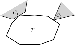
Figure 2: $\mathcal{P}$ satisfies a side contact pair $C_{1}$ and a corner contact pair $C_{2}$.

An ordered pair $(A,B)$ is a side contact pair if $A$ is a side of $Q$ and $B$ is a corner of $P$, and a corner contact pair if $A$ is a corner of $Q$ and $B$ is a side of $P$. A side contact pair or a corner contact pair is called a contact pair. We denote by $\mathcal{P}$ a homothetic copy of $P$. We say $\mathcal{P}$ satisfies a contact pair $(A,B)$ if $B$ in $\mathcal{P}$ touches $A$. See Figure 2. We say $\mathcal{P}$ is feasible if $\mathcal{P}$ is inscribed in $Q$. Note that $\mathcal{P}$ is not necessarily feasible even if $\mathcal{P}$ satisfies a contact pair.

2.3 The Algorithm of Chew and Kedem

We introduce the algorithm by Chew and Kedem. Imagine we rotate $P$ by angle $\theta$ in counterclockwise direction. Let $P_{\theta}$ be the rotated copy of $P$, and let $\mathcal{P}_{\theta}$ be a homothetic copy of $P_{\theta}$. Let $\textsf{eDT}_{\theta}$ denote the edge Delaunay triangulation of the sites in $S$ with respect to the $P_{\theta}$-distance. For a face $T$ of $\textsf{eDT}_{\theta}$, we say a $\mathcal{P}_{\theta}$ is associated to $T$ if it touches all the sites defining $T$. For $\mathcal{P}_{\theta}$ associated to $T$, the set of the elements (vertices or edges) of $\mathcal{P}_{\theta}$ touching the sites defining $T$ becomes the label of $T$. See Figure 3(a). For a site $s$ of $S$, the label of $s$ is the set of elements of $\mathcal{P}_{\theta}$’s touching $s$, for $\mathcal{P}_{\theta}$’s associated to the faces incident to $s$. See Figure 3(b).

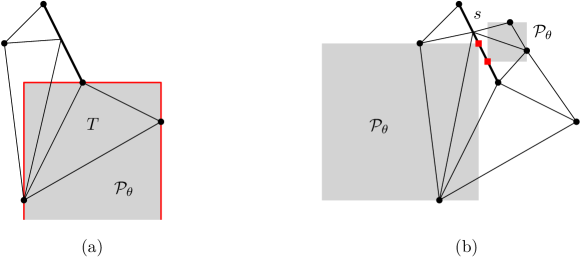
Figure 3: Labels of faces of $\textsf{eDT}_{\theta}$ and edge sites of $S$ for an axis-aligned square $P_{\theta}$. (a) The label of face $T$ is the set of red edges of $\mathcal{P}_{\theta}$. (b) The label of edge site $s$ is the set of red corners of $\mathcal{P}_{\theta}$’s.

Their algorithm classifies two possible types of changes, an edge change and a label change in $\textsf{eDT}_{\theta}$ while $\theta$ increases. In an edge change, a new generalized edge appears or an existing edge disappears. This change occurs when $\mathcal{P}_{\theta}$ touches four elements of $Q$, resulting in a flip of the diagonals in the quadrilateral formed by the four edges of $\textsf{eDT}_{\theta}$. In a label change, the label of a face in $\textsf{eDT}_{\theta}$ changes. This occurs when two or more elements of $\mathcal{P}_{\theta}$ touch the same site, but the structure of $\textsf{eDT}_{\theta}$ may be unchanged. An edge change or a label change is called a combinatorial change to $\textsf{eDT}_{\theta}$.

Their algorithm constructs and maintains a representation for $\textsf{eDT}_{\theta}$ while $\theta$ increases. It starts by creating $\textsf{eDT}_{\theta}$ at $\theta=0$. For each generalized edge in $\textsf{eDT}_{\theta}$, it determines at which orientation this edge ceases to be valid due to an interaction with its neighbors. For each face in $\textsf{eDT}_{\theta}$, the algorithm determines at which orientation the label of this face changes. An edge change is detected by checking the edges of $\textsf{eDT}_{\theta}$ and a label change is detected by checking the faces of $\textsf{eDT}_{\theta}$. The algorithm maintains the edges and faces of $\textsf{eDT}_{\theta}$ in a priority queue, ordered by the orientations at which they are changed. At each succeeding stage of the algorithm, it determines which generalized edge is the next one to disappear or which face has its label changed as $\theta$ increases. Then, it updates $\textsf{eDT}_{\theta}$ and the priority queue information for the new edge and its neighbors. Note that a new edge may change the priority for its neighbors. A priority queue can be implemented such that each operation can be done $O(\log{m})$ time, where $m$ is the maximum number of items in the queue. Since there are never more than $O(n)$ edges and faces in the queue at any one time, each priority queue operation takes time $O(\log{n})$.

For each event of a face $T$ disappearing at $\theta_{e}$, the algorithm finds the maximal interval $\mathcal{I}=[\theta_{s},\theta_{e}]$ of $\theta$ such that $T$ appears on $\textsf{eDT}_{\theta}$. To find $\mathcal{I}$ in $O(1)$ time, it stores at $T$ the orientation at which it starts to appear on $\textsf{eDT}_{\theta}$. Then it computes the orientation $\theta^{*}\in\mathcal{I}$ that maximize the area of each $\mathcal{P}_{\theta}$ that satisfies the contacts induced by $T$. Since $\mathcal{I}$ is the maximal interval, $\mathcal{P}_{\theta}$ is feasible for every $\theta\in\mathcal{I}$ but not for any $\theta\notin\mathcal{I}$ sufficiently close to $\mathcal{I}$. Thus, the algorithm considers all orientations that $\mathcal{P}_{\theta}$ is feasible and computes the placement and orientation of the largest similar copy of $P$. Note that the area function of $\mathcal{P}_{\theta}$ can be computed in $O(1)$ time and the number of $\mathcal{P}_{\theta}$ that satisfies the contacts induced by $T$ is $O(1)$. Chew and Kedem gave an upper bound $O(k^{4}n\lambda_{3}(n))$ on the combinatorial changes, and their algorithm takes $O(k^{4}n\lambda_{3}(n)\log{n})$ time [8].

3 The number of changes in $\textsf{eDT}_{\theta}$

We show that the number of combinatorial changes during the rotation is $O(k^{2}n^{2}\lambda_{4}(k))$ in this section. This directly improves the time bound for the algorithm to $O(k^{2}n^{2}\lambda_{4}(k)\log{n})$. We analyze the number of combinatorial changes in $\textsf{eDT}_{\theta}$ for a constant $k$ in Section 3.1, and then analyze the number of combinatorial changes with respect to $k$ in Section 3.2 using the observation in Section 3.1. We use the reference point $(x,y)$, the reference orientation $\theta$, and the expansion factor $\delta$ of $\mathcal{P}_{\theta}$ defined in [8], which represent a placement of $\mathcal{P}_{\theta}$ in the plane by a quadruplet $(x,y,\theta,\delta)$.

3.1 The number of changes for fixed $k$

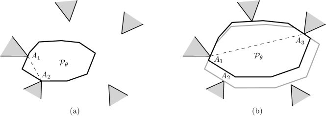
Figure 4: (a) The segment $A_{1}A_{2}$ is a reported edge with $Q_{H}=A_{2}$. (b) The segment $A_{1}A_{3}$ is an unreported edge because no hinge is involved in the segment for a feasible $\mathcal{P}_{\theta}$.

For a constant $k$, we improve the previously best upper bound $O(n\lambda_{3}(n))$ by Chew and Kedem [8] to $O(n^{2})$. A key idea is to consider the lower envelope of some functions related to the expansion factor, one for each edge and vertex of $P$, and then to analyze the lower envelope of those lower envelopes. By careful analysis on the complexities of the lower envelopes, we show that the number of combinatorial changes to $\textsf{eDT}_{\theta}$ for $\theta$ increasing from 0 to $2\pi$ is $O(n^{2})$.

An ordered pair $(Q_{H},P_{H})$ is a hinge if $Q_{H}$ is a corner of $Q$ and $P_{H}$ is a corner of $P$. For a hinge $H=(Q_{H},P_{H})$ and a contact pair $C=(A,B)$, the generalized edge connecting $Q_{H}$ and $A$ is a reported edge if there is a feasible $\mathcal{P}_{\theta}$ for some $\theta$ satisfying both $H$ and $C$. An edge of $\textsf{eDT}_{\theta}$ is an unreported edge if it is not a reported edge. See Figure 4.

Changes to the reported edges and the label changes to point sites. We count the changes to the reported edges and the changes to the labels of point sites in $\textsf{eDT}_{\theta}$ for $\theta$ increasing from $0$ to $2\pi$. We define the expansion function $E_{HC}(\theta)$ for a hinge $H$ and a contact $C$ to be the minimal expansion factor of $\mathcal{P}_{\theta}$ satisfying $H$ and $C$. For a hinge $H=(Q_{H},P_{H})$, let $\mathcal{F}_{H}$ be the set of all expansion functions satisfying $H$ and another contact pair. An expansion function $E_{HC}(\theta)$ of $\mathcal{F}_{H}$ for a contact $C=(A,B)$ appears on the lower envelope of $\mathcal{F}_{H}$ at $\theta$ if the generalized edge connecting $Q_{H}$ and $A$ is a reported edge in $\textsf{eDT}_{\theta}$. Then the number of changes to the reported edges in $\textsf{eDT}_{\theta}$ which involve $H$ is bounded by the number of breakpoints on the lower envelope of $\mathcal{F}_{H}$.

Every label change to a point site involves a hinge. See Figure 5(a). An intersection of $E_{HC_{1}}$ and $E_{HC_{2}}$ of $\mathcal{F}_{H}$ for contact pairs $C_{1}$ and $C_{2}$ appears on the lower envelope of $\mathcal{F}_{H}$ if a label change to a point site is induced by $C_{1},C_{2}$ and $H$. Then the number of label changes to the point sites in $\textsf{eDT}_{\theta}$ which involve $H$ is bounded by the number of breakpoints on the lower envelope of $\mathcal{F}_{H}$.

Proposition 4 (Proposition 3 of [8]).

Two expansion functions $E_{HC_{1}}$ and $E_{HC_{2}}$ intersect each other in at most one point in their graphs if both $C_{1}$ and $C_{2}$ are corner contact pairs, or both are side contact pairs. If one is a corner contact pair and the other is a side contact pair, $E_{HC_{1}}$ and $E_{HC_{2}}$ intersect in at most two points in their graphs.

Let $v_{i}$ and $e_{i}$ denote the vertices and edges of $P$ for $i=1,\dots,k$. For each $i=1\dots k$, let $\mathcal{C}_{1i}=\{(e,v_{i})\mid\text{$e$ is an edge of $Q$}\}$ be the set of side contact pairs and let $\mathcal{C}_{2i}=\{(v,e_{i})\mid\text{$v$ is a vertex of $Q$}\}$ be the set of corner contact pairs. Let $\mathcal{F}_{ji}=\{E_{HC}\mid C\in\mathcal{C}_{ji}\}$ for $j=1,2$.

Lemma 5.

The number of breakpoints on the lower envelope of $\mathcal{F}_{ji}$ is $O(n)$ for each $j=1,2$ and $i=1,\dots,k$.

Proof.

The number of breakpoints on the lower envelope of $\mathcal{F}_{1i}$ is $O(n)$ for each $i$ since $E_{HC_{1}}$ and $E_{HC_{2}}$ intersect only at the boundaries of their intervals for $C_{1},C_{2}\in\mathcal{C}_{1i}$.

Consider now the number of breakpoints on the lower envelope of $\mathcal{F}_{2i}$. Two expansion functions $E_{HC_{1}}$ and $E_{HC_{2}}$ intersect in at most one point for $C_{1},C_{2}\in\mathcal{C}_{2i}$. Also, $E_{HC}$ has the same length of domain for all $C\in\mathcal{C}_{2i}$. Thus, the number of breakpoints on the lower envelope of $\mathcal{F}_{2i}$ is $O(n)$ by Lemma 1. ∎

From Corollary 3, Proposition 4, and Lemma 5, we achieve an upper bound on the number of breakpoints on the lower envelope of $\mathcal{F}_{H}$.

Lemma 6.

The number of breakpoints on the lower envelope of $\mathcal{F}_{H}$ is $O(\lambda_{3}(k)n)$.

Proof.

Let $\mathcal{F}_{j}=\{f_{j1},\dots,f_{jk}\}$ for $j=1,2$, where $f_{ji}$ is the lower envelope of $\mathcal{F}_{ji}$ for each $i=1,\dots,k$ and $j=1,2$. Let $\mathcal{L}_{j}$ denote the lower envelope of $\mathcal{F}_{j}$. Then, the lower envelope of $\mathcal{F}_{H}$ is the lower envelope of $\mathcal{L}_{1}$ and $\mathcal{L}_{2}$. The number of breakpoints on $\mathcal{L}_{j}$ is $O(\lambda_{3}(k)n)$ for $j=1,2$ by Corollary 3, Proposition 4, and Lemma 5. The number of breakpoints on the lower envelope of $\mathcal{F}_{H}$ is also $O(\lambda_{3}(k)n)$, because two continuous pieces, one from $\mathcal{L}_{1}$ and one from $\mathcal{L}_{2}$, intersect at most two points by Proposition 4. ∎

By Lemma 6, the number of changes to the reported edges and the number of label changes to the point sites are $O(k\lambda_{3}(k)n^{2})$.

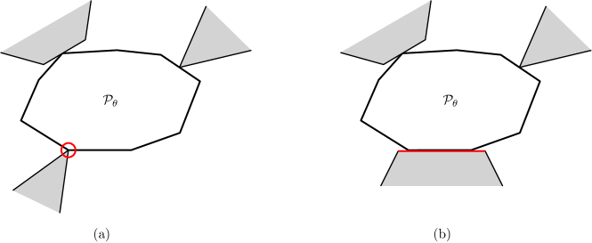
Figure 5: The label changes to the red sites. (a) Label change to a point site (hinge). (b) Label change to an edge site.

Label changes to edge sites. We count the changes to the labels of edge sites in $\textsf{eDT}_{\theta}$ for $\theta$ increasing from 0 to $2\pi$. Imagine we fix an edge $e$ of $Q$ and an edge $g$ of $P$. See Figure 5(b). Then, the number of label changes to edge site $e$ with $g$ is $O(n)$ because the edge site and the edge of $P$ are aligned. The number of label changes to all edge sites is $O(kn^{2})$.

Changes to unreported edges. We count the changes to unreported edges using the numbers of changes to the reported edges and to the labels, and Lemma 7.

Lemma 7 (Lemma 2 of [8]).

Every edge of $\textsf{eDT}_{\theta}$ is either a reported edge or a diagonal in a convex $l$-gon, $l\leq 3k$, whose sides are either reported edges or portions of edge sites.

Let $G_{\theta}$ be the graph whose edges are the reported edges in $\textsf{eDT}_{\theta}$ and portions of edge sites in Lemma 7. We count the changes to the unreported edges which are diagonals in a face of $G_{\theta}$ for an interval of $\theta$ with no label change to $\textsf{eDT}_{\theta}$. Observe that no combinatorial change occurs to $G_{\theta}$ for the interval. Any change to an unreported edge involves four sites lying on a face boundary of $G_{\theta}$. There are at most four changes for a group of four sites. We describe the details on this bound in Section 4. Since each face has at most $3k$ edges by Lemma 7, there are at most $\binom{3k}{4}$ such groups. Since $O(k^{4})$ changes occur to the unreported edges for the boundary of a face $g$ of $G_{\theta}$ during an interval of $\theta$ with no label change to the faces of $\textsf{eDT}_{\theta}$ intersecting $g$, there are $O(k^{5}n^{2}\lambda_{3}(k))$ combinatorial changes to $\textsf{eDT}_{\theta}$.

Theorem 8.

For a polygonal domain $Q$ of size $n$ and a convex $k$-gon $P$, the number of combinatorial changes to $\textsf{eDT}_{\theta}$ for $\theta$ increasing from 0 to $2\pi$ is $O(n^{2})$ for a constant $k$.

3.2 The number of changes with respect to $k$

We now consider $k$ as a variable and bound the number of changes to $\textsf{eDT}_{\theta}$. Since each triangular face in $\textsf{eDT}_{\theta}$ is defined by three elements (edges or vertices) of $P$, we choose three elements of $P$ then use their convex hull in the counting. Then the number of faces in $\textsf{eDT}_{\theta}$ for all these convex hulls is at most $O(k^{3}n^{2})$ for $\theta$ increasing from 0 to $2\pi$, by Theorem 8. Let $\mathcal{T}$ be the set of all faces of $\textsf{eDT}_{\theta}$ for the convex hull $P^{\prime}$ for three elements $B_{1},B_{2},B_{3}$ of $P$ such that the contact pairs inducing the face have $B_{1},B_{2}$, and $B_{3}$ as their elements.

Consider two faces $T$ and $T^{\prime}$ of $\textsf{eDT}_{\theta}$ for two distinct orientations $\theta=\theta_{1}$ and $\theta=\theta_{2}$ with $\theta_{1}<\theta_{2}$ that are defined by the same sites. We consider $T$ and $T^{\prime}$ as distinct faces if there is any change to $T$ or $T^{\prime}$ in $\textsf{eDT}_{\theta}$ for $\theta$ from $\theta_{1}$ to $\theta_{2}$. For a face $T\in\mathcal{T}$, let $C(T)$ be the set of contact pairs which defines $T$, and let $I(T)$ be the interval of $\theta$ at which $T$ appears to $\textsf{eDT}_{\theta}$.

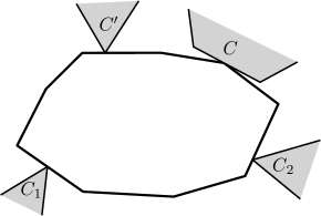
Figure 6: The combinatorial change induced by $C_{1},C_{2},C$, and $C^{\prime}$.

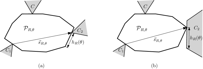
Figure 7: $\mathcal{P}_{R,\theta},\vec{s}_{R,\theta},$ and $h_{R}(\theta)$ for a restricted contact pair $R=(C,I)$ and $\theta$. Let $h_{R}(\theta)$ be the distance from the clockwise endpoint (with respect to $\vec{s}_{R,\theta}$) of the side element of $C_{2}$ to point element of $C_{2}$. (a) $h_{R}(\theta)$ when $C_{2}$ is a corner contact. (b) $h_{R}(\theta)$ when $C_{2}$ is a side contact.

For any two fixed contact pairs $(C_{1},C_{2})$, we count the combinatorial changes involving $(C_{1},C_{2})$, and other contact pairs $C$ and $C^{\prime}$ given in counterclockwise order $C_{1},C_{2},C,$ and $C^{\prime}$ along the boundary of $P$. See Figure 6. Note that for $(C_{1},C_{2})$ with $C_{i}=(A_{i},B_{i})$ for $i=1,2$, we do not count the combinatorial changes for the pair if $A_{1}=A_{2}$ or $B_{1}=B_{2}$. The combinatorial changes not counted are counted for other two fixed contact pairs.

We use $(C,I)$ to denote a contact pair $C$ restricted to an interval $I$ of $\theta$. Let $\mathcal{R}$ be the set of restricted contact pairs $(C,I)$ such that $C(T)=\{C_{1},C_{2},C\}$ and $I=I(T)$ for a face $T\in\mathcal{T}$, and $C_{1},C_{2},C$ appear in counterclockwise order along $P$. For a fixed restricted contact pair $R\in\mathcal{R}$ and $\theta\in I$ for $R=(C,I)$, let $\mathcal{P}_{R,\theta}$ denote the homothet of $P_{\theta}$ which satisfies $C_{1},C_{2}$, and $C$. We use $\vec{s}_{R,\theta}$ to denote the ray from the point element of $C_{1}$ to the point element of $C_{2}$ in $\mathcal{P}_{R,\theta}$. Let $h_{R}(\theta)$ be the function that denotes the distance from the clockwise endpoint (with respect to $\vec{s}_{R,\theta}$) of the side element of $C_{2}$ to point element of $C_{2}$ with respect to $\mathcal{P}_{R,\theta}$. See Figure 7.

Figure 8: Partitioning $\mathcal{R}$ by classes using the intersections of function graphs of $\mathcal{F}$. Class $\mathcal{R}^{\prime}$ has $R$ and $R^{\prime}$, and there is a sequence $f_{1},\dots,f_{j}$ with $f_{1}=h_{R},f_{j}=h_{R^{\prime}}$ such that $f_{j^{\prime}}$ and $f_{j^{\prime}+1}$ intersect each other for every $j^{\prime}=1,\dots,j-1$.

Observe that $h_{R}$ is a partially defined continuous function on $R\in\mathcal{R}$. Let $\mathcal{F}=\{h_{R}\mid R\in\mathcal{R}\}$. Two restricted contact pairs $R,R^{\prime}\in\mathcal{R}$ are in the same class if and only if there is a subset $\{f_{1},\dots,f_{j}\}\subset\mathcal{F}$ with $f_{1}=h_{R},f_{j}=h_{R^{\prime}}$ such that $f_{j^{\prime}}$ and $f_{j^{\prime}+1}$ intersect each other for every $j^{\prime}=1,\dots,j-1$. Figure 8 illustrates the classes of $\mathcal{R}$.

If a combinatorial change is induced by $C_{1},C_{2},C,$ and $C^{\prime}$ at $\theta$, we have $h_{R}(\theta)=h_{R^{\prime}}(\theta)$ for distinct restricted contact pairs $R=(C,I)$ and $R^{\prime}=(C^{\prime},I^{\prime})$. See Figure 6. Let $\mathcal{R^{\prime}}\subset{\mathcal{R}}$ be a subclass of $\mathcal{R}$ and let $\mathcal{F}^{\prime}=\{h_{R}\mid R\in\mathcal{R^{\prime}}\}$. We verify that if $\mathcal{P}_{R,\theta}$ is feasible, then $h_{R}(\theta)$ appears on the lower envelope or upper envelope of $\mathcal{F}^{\prime}$.

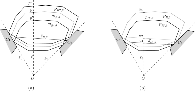
Figure 9: Proof of Lemma 9.

Lemma 9.

Let $R,R^{\prime},R^{\prime\prime}\in\mathcal{R}$ be the restricted contact pairs in the same class. If $h_{R^{\prime}}(\theta)<h_{R}(\theta)<h_{R^{\prime\prime}}(\theta)$, then $\mathcal{P}_{R,\theta}$ is not feasible.

Proof.

Let $R=(C,I),R^{\prime}=(C^{\prime},I^{\prime})$, and $R^{\prime\prime}=(C^{\prime\prime},I^{\prime\prime})$. Let $\ell_{1}$ be the line through the edge element of $C_{1}$, $\ell_{2}$ be the line through the edge element of $C_{2}$, and $O$ be the intersection of $\ell_{1}$ and $\ell_{2}$ unless they are parallel. For a fixed point $\bar{p}$ on the boundary of $P$, let $p^{\prime},p,$ and $p^{\prime\prime}$ be the points on the boundaries of $\mathcal{P}_{R^{\prime},\theta},\mathcal{P}_{R,\theta},$ and $\mathcal{P}_{R^{\prime\prime},\theta}$, respectively, corresponding to $\bar{p}$. Then $p^{\prime},p,$ and $p^{\prime\prime}$ are on the same line $\ell$ and the order of $p^{\prime},p,$ and $p^{\prime\prime}$ (with $p$ in between $p^{\prime}$ and $p^{\prime\prime}$) on $\ell$ remains the same for any choice of $\bar{p}$ because $h_{R^{\prime}}(\theta)<h_{R}(\theta)<h_{R^{\prime\prime}}(\theta)$. Observe that $\ell$ passes through $O$ (if exists) and crosses both $\vec{s}_{R,\theta}$ and $\vec{s}_{R^{\prime\prime},\theta}$. See Figure 9(a).

Let $p_{R^{\prime},\theta}$ be the position of the point element of $C^{\prime}$ in $\mathcal{P}_{R^{\prime},\theta}$. Let $\ell_{3}$ be the line through $O$ and $p_{R^{\prime},\theta}$ if $O$ exists. Otherwise, let $\ell_{3}$ be the line through $p_{R^{\prime},\theta}$ and parallel to $\ell_{1}$ and $\ell_{2}$. Let $a_{1}=\vec{s}_{R^{\prime},\theta}\cap\ell_{3},a_{2}=\vec{s}_{R,\theta}\cap\ell_{3}$ and let $a_{3}$ be the point on the boundary of $\mathcal{P}_{R,\theta}$ corresponding to $p_{R^{\prime},\theta}$ on $\mathcal{P}_{R^{\prime},\theta}$. Without loss of generality, assume that $\ell_{3}$ is vertical, and $p_{R^{\prime},\theta}$ lies above $a_{1}$.

Consider the case that $p_{R^{\prime},\theta}$ lies below $a_{3}$. See Figure 9(b). We show that $p_{R^{\prime},\theta}$ does not lie on the segment $a_{1}a_{2}$. Since $R^{\prime},R$ are in the same class, there is a subset $\{f_{1},\dots,f_{j}\}\subset\mathcal{F}$ with $f_{1}=h_{R^{\prime}},f_{j}=h_{R}$ such that $f_{j^{\prime}}$ and $f_{j^{\prime}+1}$ intersect each other for every $j^{\prime}=1,\dots,j-1$. Let $R_{j^{\prime}}=(C_{j^{\prime}},I_{j^{\prime}})$ be the restricted contact pair with angle interval $I_{j^{\prime}}$ such that $h_{R_{j^{\prime}}}=f_{j^{\prime}}$ for $j^{\prime}=1,\dots,j$. Let $\mathcal{P}^{\prime}_{R_{j^{\prime}},\theta^{\prime}}$ be the rotated and scaled copy of the convex hull of $B_{1},B_{2}$, and $B^{\prime}$ of $C_{j^{\prime}}=(A^{\prime},B^{\prime})$, satisfying $C_{1},C_{2}$ and $C_{j^{\prime}}$. Then $\vec{s}_{R_{j^{\prime}},\theta^{\prime}}$ never intersects $p_{R^{\prime},\theta}$ for any $\theta^{\prime}\in I_{j^{\prime}}$ and $j^{\prime}=1,\dots,j$ since $p_{R^{\prime},\theta}$ does not lie in the interior of $\mathcal{P}^{\prime}_{R_{j^{\prime}},\theta^{\prime}}$ but $\vec{s}_{R_{j^{\prime}},\theta^{\prime}}$ is contained in the interior of $\mathcal{P}^{\prime}_{R_{j^{\prime}},\theta^{\prime}}$. Let $\theta_{j^{\prime}}\in I_{j^{\prime}}$ be one of the orientations at which an intersection of $f_{j^{\prime}}$ and $f_{j^{\prime}+1}$ occurs for each $j^{\prime}=1,\dots,j-1$. Then, $\vec{s}_{R_{j^{\prime}},\theta_{j^{\prime}-1}}$ can be translated continuously to $\vec{s}_{R_{j^{\prime}},\theta_{j^{\prime}}}$ for $\theta$ from $\theta_{j^{\prime}-1}$ to $\theta_{j^{\prime}}$ for each $j^{\prime}=2,\dots,j-1$. Also, $\vec{s}_{R^{\prime},\theta}$ can be translated continuously to $\vec{s}_{R^{\prime},\theta_{1}}$, and $\vec{s}_{R,\theta_{j-1}}$ can be translated continuously to $\vec{s}_{R,\theta}$. If $p_{R^{\prime},\theta}$ lies on $a_{1}a_{2}$, $p_{R^{\prime},\theta}$ lies on $\vec{s}_{R_{j^{\prime}},\theta^{\prime}}$ for some $j^{\prime}=1,\dots,j$ and $\theta^{\prime}\in I_{j^{\prime}}$. This contradicts to the fact that $\vec{s}_{R_{j^{\prime}},\theta^{\prime}}$ never intersects $p_{R^{\prime},\theta}$. Thus, $p_{R^{\prime},\theta}$ lies above $a_{1}a_{2}$. Then $p_{R^{\prime},\theta}$ lies in the interior of $a_{2}a_{3}$, that is, $p_{R^{\prime},\theta}$ lies in the interior of $\mathcal{P}_{R,\theta}$, and therefore $\mathcal{P}_{R,\theta}$ is not feasible.

Now consider the case that $p_{R^{\prime},\theta}$ lies above $a_{3}$. Then by an argument similar to the one for the previous case, we can show that $p_{R^{\prime\prime},\theta}$ is contained in the interior of $\mathcal{P}_{R,\theta}$, where $p_{R^{\prime\prime},\theta}$ is the position of the point element of $C^{\prime\prime}$ in $\mathcal{P}_{R^{\prime\prime},\theta}$. Therefore $\mathcal{P}_{R,\theta}$ is not feasible. ∎

Let $\mathcal{R^{\prime}}_{1i}$ be the subset of $\mathcal{R^{\prime}}$ such that $R=(C,I)\in\mathcal{R^{\prime}}$ belongs to $\mathcal{R^{\prime}}_{1i}$ if $C=(e,v_{i})$ is a side contact pair for some edge $e\in Q$. Let $\mathcal{R^{\prime}}_{2i}$ be the subset of $\mathcal{R^{\prime}}$ such that $R=(C,I)\in\mathcal{R^{\prime}}$ belongs to $\mathcal{R^{\prime}}_{2i}$ if $C=(v,e_{i})$ is a corner contact pair for some vertex $v\in Q$. Suppose that $\left\lvert\mathcal{R^{\prime}}\right\rvert=m$ and $\left\lvert\mathcal{R^{\prime}}_{1i}\right\rvert=m_{1i},\left\lvert\mathcal{R^{\prime}}_{2i}\right\rvert=m_{2i}$ for $i=1,\dots,k$. Let $\mathcal{F}^{\prime}_{ji}=\{h_{R}\mid R\in\mathcal{R^{\prime}}_{ji}\}$ for $j=1,2$. First, we count the breakpoints on the lower envelope of $\mathcal{F}^{\prime}_{1i}$ and the lower envelope $\mathcal{F}^{\prime}_{2i}$. The number of breakpoints on the lower envelope of $\mathcal{F}^{\prime}_{1i}$ is $O(m_{1i})$ since $h_{R}$ and $h_{R^{\prime}}$ can intersect only at the boundaries of their intervals for $R,R^{\prime}\in\mathcal{R^{\prime}}_{1i}$. Let $d_{i}$ be the number of intersections of the function graphs of $\mathcal{F}^{\prime}_{2i}$, and let $d=\sum_{i=1}^{k}d_{i}$. Then the number of breakpoints on the lower envelope of $\mathcal{F}^{\prime}_{2i}$ is $O(m_{2i}+d_{i})$.

Lemma 10.

The number of breakpoints on the lower envelope of $\mathcal{F}^{\prime}_{1i}$ is $O(m_{1i})$ and $\mathcal{F}^{\prime}_{2i}$ is $O(m_{2i}+d_{i})$ for each $i=1,\dots,k$.

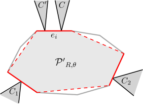
Figure 10: For $R=(C,I)$ and $R^{\prime}=(C^{\prime},I^{\prime})$ in $\mathcal{R^{\prime}}_{2i}$, and orientation $\theta$ with $h_{R}(\theta)=h_{R^{\prime}}(\theta)$, there exists a rotated and scaled copy of the convex hull of $B_{1},B_{2}$, and $e_{i}$, satisfying $C_{1},C_{2}$ and $C,C^{\prime}$, and feasible. The intersection $h_{R}(\theta)=h_{R^{\prime}}(\theta)$ corresponds to a combinatorial change to $\textsf{eDT}_{\theta}$ for the convex hull of $B_{1},B_{2},$ and $e_{i}$.

Observe that each intersection of the function graphs of $\mathcal{F}^{\prime}_{2i}$ corresponds to a combinatorial change to eDT for the convex hull of $B_{1},B_{2},$ and $e_{i}$. See Figure 10. By Lemma 9, every combinatorial change appears on the lower envelope or upper envelope of $\mathcal{F}^{\prime}$. Here, we describe the case for the lower envelope of $\mathcal{F}^{\prime}$. We count the breakpoints of certain types on the lower envelope of $\mathcal{F}^{\prime}$. The combinatorial changes corresponding to the breakpoints not counted here will be counted for other choices of the fixed pair. We use $(a,b)$-change to denote a combinatorial change induced by $a$ side contact pairs and $b$ corner contact pairs.

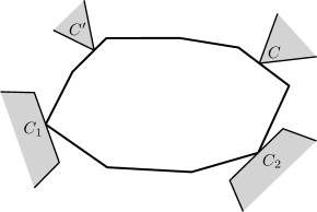
Figure 11: The $(2,2)$-change induced by $C_{1},C_{2},C$ and $C^{\prime}$ is counted when $C_{2}$ and $C$ are chosen as the fixed pair.

Two side contact pairs. We count only $(4,0)$-changes in this case. We count $(3,1)$ and $(2,2)$-changes appearing on the lower envelope in other choices of the fixed pair. See Figure 11. By Corollary 3 and Lemma 10, the number of breakpoints on the lower envelope of $\mathcal{F}^{\prime}_{1}=\{f_{i}\mid i=1,\dots,k\}$ is $\sum_{i=1}^{k}O(m_{1i}\lambda_{4}(k)/k)=O(m\lambda_{4}(k)/k)$, where $f_{i}$ is the lower envelope of $\mathcal{F}^{\prime}_{1i}$. In Section 4, we show that any two continuous pieces in $\mathcal{F}^{\prime}_{1}$ intersect each other in at most two points. Since each $(4,0)$-change corresponds to a breakpoint on the lower envelope of $\mathcal{F}^{\prime}_{1}$, the number of $(4,0)$-changes is $O(m\lambda_{4}(k)/k)$.

Two corner contact pairs. We count only $(0,4)$-combinatorial changes in this case. Other changes are counted for other choices of the fixed pair. By Corollary 3 and Lemma 10, the number of breakpoints on the lower envelope of $\mathcal{F}^{\prime}_{2}=\{f_{i}\mid i=1,\dots,k\}$ is $\sum_{i=1}^{k}O((m_{2i}+d_{i})\lambda_{4}(k)/k)=O((m+d)\lambda_{4}(k)/k)$, where $f_{i}$ is the lower envelope of $\mathcal{F}^{\prime}_{2i}$. In Section 4, we show that any two continuous pieces in $\mathcal{F}^{\prime}_{2}$ intersect each other in at most two points. Since each $(0,4)$-change corresponds to a breakpoint of the lower envelope of $\mathcal{F}^{\prime}_{2}$, the number of $(0,4)$-changes is $O((m+d)\lambda_{4}(k)/k)$.

One side contact pair and one corner contact pair. We count all combinatorial changes other than $(4,0)$-changes and $(0,4)$-changes. First, we count the breakpoints of the lower envelope of $\mathcal{F}^{\prime}_{1}=\{h_{R}\mid R\in\bigcup_{i=1}^{k}\mathcal{R^{\prime}}_{1i}\}$ and of the lower envelope of $\mathcal{F}^{\prime}_{2}=\{h_{R}\mid R\in\bigcup_{i=1}^{k}\mathcal{R^{\prime}}_{2i}\}$, then count the breakpoints of the lower envelope of $\mathcal{F}^{\prime}_{1}\cup\mathcal{F}^{\prime}_{2}$. In Section 4, we show that any two continuous pieces, both from either $\mathcal{F}^{\prime}_{1}$ or $\mathcal{F}^{\prime}_{2}$, intersect each other in at most two points. The number of breakpoints of the lower envelope of $\mathcal{F}^{\prime}_{1}$ can be computed in the same way as for counting $(4,0)$-changes, and the result is $O(m\lambda_{4}(k)/k)$. The number of breakpoints of the lower envelope of $\mathcal{F}^{\prime}_{2}$ can be computed in the same way as for counting $(0,4)$-changes, and the result is $O((m+d)\lambda_{4}(k)/k)$. The number of breakpoints of the lower envelope of $\mathcal{F}^{\prime}$ is $O((m+d)\lambda_{4}(k)/k)$, since the number of breakpoints of the lower envelope of $\mathcal{F}^{\prime}_{1}$ and of the lower envelope of $\mathcal{F}^{\prime}_{2}$ is $O((m+d)\lambda_{4}(k)/k)$, and any two continuous pieces, one from $\mathcal{F}^{\prime}_{1}$ and one from $\mathcal{F}^{\prime}_{2}$, intersect each other in at most four points by Section 4. Thus, the number the combinatorial changes for the fixed contact pair is $O((m+d)\lambda_{4}(k)/k)$.

Consider the sum $\sigma$ of the complexity $|\mathcal{F}^{\prime}|=m$ of $\mathcal{F}^{\prime}$ over all classes for a fixed pair. Then the total sum of $\sigma$’s for all enumerations of fixed pairs is $O(k^{3}n^{2})$ since $|\mathcal{T}|=O(k^{3}n^{2})$. Similarly, consider the sum $\xi$ of the number of intersections ($d$ in the complexities in the previous paragraphs) over all classes for a fixed pair. Then the total sum of $\xi$’s for all enumerations of fixed pairs is $O(k^{3}n^{2})$ since $\xi$ is bounded by the number of combinatorial changes to $\textsf{eDT}_{\theta}$ for the convex hulls of three elements of $P$. Therefore, we conclude with the following theorem.

Theorem 11.

For a polygonal domain $Q$ of size $n$ and a convex $k$-gon $P$, the number of combinatorial changes to the edge Delaunay triangulation of $Q$ under $P_{\theta}$-distance for $\theta$ increasing from 0 to $2\pi$ is $O(k^{2}n^{2}\lambda_{4}(k))$.

Theorem 11 directly improves the time complexity of the algorithm by Chew and Kedem.

Corollary 12.

Given a polygonal domain $Q$ of size $n$ and a convex $k$-gon $P$, we can find a largest similar copy of $P$ that can be inscribed in $Q$ in $O(k^{2}n^{2}\lambda_{4}(k)\log{n})$ time using $O(kn)$ space.

4 The number of critical orientations for four contact pairs

The orientation $\theta$ at which a combinatorial change to $\textsf{eDT}_{\theta}$ occurs is called a critical orientation. We consider the critical orientations $\theta$ at which $\mathcal{P}_{\theta}$ has contact with four contact pairs. We count the number of critical orientations for each $(a,b)$-change type. The number of critical orientations of $(0,4)$-change is 2, which is shown in Appendix B of [8]. So in this section, we count the critical orientations for the other types of combinatorial changes. The following table summarizes the results.

Types of $(a,b)$-change	$(4,0)$	$(3,1)$	$(2,2)$	$(1,3)$	$(0,4)$
Number of critical orientations	1	2	4	2	2

4.1 Common intersection and directed angles

We need some technical lemmas before computing the critical orientations. For any two lines $\ell$ and $\ell^{\prime}$ crossing each other in the plane, the directed angle, denoted by $\measuredangle{(}\ell,\ell^{\prime})$, is the angle from $\ell$ to $\ell^{\prime}$, measured counterclockwise around their intersection point. This definition can be extended for three points $A,O,$ and $B$, and we use $\measuredangle{AOB}=\measuredangle{(}AO,BO)$ to denote the directed angle from the line through $AO$ to the line through $BO$, measured counterclockwise around $O$. There are some properties of directed angles which we use in this section.

Proposition 13.

The following properties hold:

1. For any three points $A,B,$ and $O$, we have $\measuredangle{AOB}=-\measuredangle{BOA}$ modulo $\pi$.

2. For any four points $A,B,X,$ and $Y$ such that no three of them are collinear, they are concyclic if and only if $\measuredangle{XAY}=\measuredangle{XBY}$ modulo $\pi$.

3. For any three lines $\ell_{1},\ell_{2},$ and $\ell_{3}$ such that no two lines are parallel, we have $\measuredangle{(}\ell_{1},\ell_{2})+\measuredangle{(}\ell_{2},\ell_{3})=\measuredangle{(}\ell_{1},\ell_{3})$ modulo $\pi$. For any four points $A,B,C,$ and $O$, we have $\measuredangle{AOB}+\measuredangle{BOC}=\measuredangle{AOC}$ modulo $\pi$.

4. For any three lines $\ell_{1},\ell_{2},$ and $\ell_{3}$ such that no two lines are parallel, we have $\measuredangle{(}\ell_{1},\ell_{2})+\measuredangle{(}\ell_{2},\ell_{3})+\measuredangle{(}\ell_{3},\ell_{1})=0$ modulo $\pi$.

Figure 12: Some possible configurations of Lemmas 14 and 15.

See Figure 12 for an illustration of Lemmas 14 and 15.

Lemma 14 (Miquel’s Theorem [9]).

Let $A,B$, and $C$ be the corners of a triangle, and let $D,E$, and $F$ be the points on the lines containing $CB$, $AC$, and $AB$, respectively. Then the three circumcircles to triangles $EAF$, $FBD$ and $DCE$ have a common point of intersection.

Lemma 15.

Let $A,B$, and $C$ be the corners of a triangle, and let $D,E$, and $F$ be the points on the lines containing $CB$, $AC$, and $AB$, respectively. Let $G$ be the intersection of three circumcircles to triangles $EAF$, $FBD$ and $DCE$, and let $\measuredangle{BAC}=\alpha,\measuredangle{CBA}=\beta,\measuredangle{ACB}=\gamma,\measuredangle{EDF}=\alpha^{\prime},\allowbreak\measuredangle{FED}=\beta^{\prime},\measuredangle{DFE}=\gamma^{\prime}$ modulo $\pi$ for fixed angles $\alpha,\beta,\gamma,\alpha^{\prime},\beta^{\prime}$, and $\gamma^{\prime}$.

1. $\measuredangle{AGB}=\gamma-\alpha^{\prime}-\beta^{\prime},\measuredangle{BGC}=\alpha-\beta^{\prime}-\gamma^{\prime}$, and $\measuredangle{CGA}=\beta-\gamma^{\prime}-\alpha^{\prime}$ modulo $\pi$, regardless of $\measuredangle{EFA}$.

2. If $ABC$ or $DEF$ remains unchanged while $\measuredangle{EFA}$ is changing, $G$ remains unchanged.

3. $\measuredangle{GDF},\measuredangle{EDG},\measuredangle{GED},\measuredangle{FEG},\measuredangle{GFE},$ and $\measuredangle{DFG}$ remain unchanged while $\measuredangle{EFA}$ is changing.

Proof.

See Figure 12 for an illustration.

1. Suppose that $\measuredangle{GDF}=\alpha_{1},\measuredangle{EDG}=\alpha_{2},\measuredangle{GED}=\beta_{1},\measuredangle{FEG}=\beta_{2},\measuredangle{GFE}=\gamma_{1}$, and $\measuredangle{DFG}=\gamma_{2}$ modulo $\pi$. Then,

   $$\alpha=\beta_{2}+\gamma_{1}, \beta=\gamma_{2}+\alpha_{1}, \gamma=\alpha_{2}+\beta_{1}, (\text{by Proposition~{}}\ref{prop:directed_angle}.2)$$

   $$\alpha^{\prime}=\alpha_{1}+\alpha_{2}, \beta^{\prime}=\beta_{1}+\beta_{2}, \gamma^{\prime}=\gamma_{1}+\gamma_{2}$$

   modulo $\pi$. Using the equations above, we have

   $$\measuredangle{AGB} =-\measuredangle{GBA}-\measuredangle{BAG}=-\measuredangle{GBF}-\measuredangle{FAG}=-\measuredangle{GDF}-\measuredangle{FEG}$$

   $$=-\alpha_{1}-\beta_{2}=\gamma-\alpha^{\prime}-\beta^{\prime}$$

   modulo $\pi$. We can show $\measuredangle{BGC}=\alpha-\beta^{\prime}-\gamma^{\prime}$, and $\measuredangle{CGA}=\beta-\gamma^{\prime}-\alpha^{\prime}$ modulo $\pi$ in the same way.

2. Suppose that triangle $ABC$ remain unchanged while $\measuredangle{EFA}$ is changing. By Lemma 15.1, the circumcircles to triangles $ABG,BCG,$ and $CAG$ remain unchanged. Thus, their common intersection $G$ also remains unchanged. When the triangle $DEF$ remains unchanged, $G$ also remains unchanged since the circumcircles to triangles $EAF,FBD,$ and $DCE$ remain unchanged.

3. It is deduced by Lemma 15.2.

∎

4.2 Counting critical orientations

Now we count the critical orientations which is induced by the same set of contact pairs. To do this, we count the orientations $\theta$ at which $\mathcal{P}_{\theta}$ satisfies the four contact pairs, $C_{i}=(A_{i},B_{i})$ for $i=1,\ldots,4$. We consider each type of $(a,b)$-changes in the following.

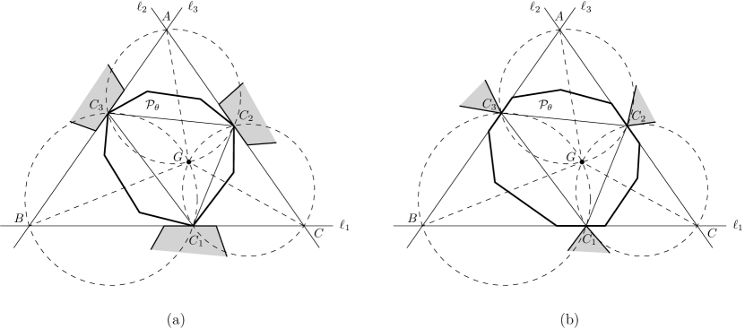
Figure 13: (a) $\mathcal{P}_{\theta}$ satisfies the side contact pairs $C_{i}=(A_{i},B_{i})$ for $i=1,2,3$. (b) $\mathcal{P}_{\theta}$ satisfies the corner contact pairs $C_{i}=(A_{i},B_{i})$ for $i=1,2,3$.

$(4,0)$-changes and $(3,1)$-changes. Suppose that $C_{1},C_{2}$, and $C_{3}$ are side contact pairs and $\mathcal{P}_{\theta}$ satisfies them. Let $\ell_{i}$ be the line through $A_{i}$ for each $i=1,2,3$, and let $A=\ell_{2}\cap\ell_{3},B=\ell_{1}\cap\ell_{3}$, and $C=\ell_{1}\cap\ell_{2}$. By Lemma 14, the circumcircles to triangles $AB_{2}B_{3},BB_{3}B_{1},$ and $CB_{1}B_{2}$ have a common intersection point, denoted by $G$. See Figure 13(a). By Lemma 15.2, $G$ remains unchanged for any $\theta$ since $A,B,$ and $C$ remain unchanged. Also, $\measuredangle{B_{2}B_{1}G}$ and $\measuredangle{GB_{2}B_{1}}$ remain unchanged by Lemma 15.3.

We use $\overrightarrow{XY}$ to denote the vector from point $X$ to point $Y$. Let $\Phi_{s,\vartheta}$ denote the affine transformation with scale factor $s$ and rotation angle $\vartheta$ in counterclockwise direction. Then there exist $s$ and $\vartheta$ such that $\overrightarrow{GB_{2}}=\Phi_{s,\vartheta}\overrightarrow{GB_{1}}$ for every $\mathcal{P}_{\theta}$ satisfying $C_{1},C_{2}$, and $C_{3}$. For a vertex $V$ of $\mathcal{P}$, $\overrightarrow{GV}=t_{1}\overrightarrow{GB_{1}}+t_{2}\overrightarrow{GB_{2}}$ for constants $t_{1}$ and $t_{2}$. Therefore, $\overrightarrow{GV}=\Phi_{s^{\prime},\vartheta^{\prime}}\overrightarrow{GB_{1}}$ for some $s^{\prime}$ and $\vartheta^{\prime}$, and the trace of $V$ is a line segment.

If $C_{4}$ is also a side contact pair, the traces of $B_{4}$ and $A_{4}$ intersect each other at most once since the trace of $B_{4}$ is a line segment. Therefore, there is at most one critical orientation for a $(4,0)$-change. Consider the case that $C_{4}$ is a corner contact pair. Assume that $B_{4}=V_{1}V_{2}$, for vertices $V_{1}$ and $V_{2}$ of $P$. Since the trace of $V_{1}$ is a segment, $\overrightarrow{GV_{1}}$ can be parametrized to $t\vec{v}_{1}+\vec{c}_{1}$ for some $\vec{v}_{1},\vec{c}_{1}$ and $t=t(\theta)$. Since $GV_{2}=\Phi_{s_{1},\vartheta_{1}}\overrightarrow{GV_{1}}$ for some $s_{1}$ and $\vartheta_{1}$, $\overrightarrow{GV_{2}}$ can be parametrized to $t\vec{v}_{2}+\vec{c}_{2}$ for some $\vec{v}_{2},\vec{c}_{2}$ and $t=t(\theta)$. If $\mathcal{P}_{\theta}$ satisfies $C_{4}$, we have $\overrightarrow{GA_{4}}=t^{\prime}\overrightarrow{GV_{1}}+(1-t^{\prime})\overrightarrow{GV_{2}}=t^{\prime}t(\vec{v}_{1}-\vec{v}_{2})+t^{\prime}(\vec{c}_{1}-\vec{c}_{2})+t\vec{v}_{2}+\vec{c}_{2}$ for some $t$ and $t^{\prime}\in[0,1]$. Thus, we obtain two equations for $t^{\prime}$ and $t$ in $x$- and $y$-coordinates. By eliminating $t^{\prime}$ using these two equations, we obtain a quadratic equation for $t$ which has at most two solutions. Therefore, there are at most two critical orientations for a $(3,1)$-change.

$(1,3)$-changes. Suppose that $C_{1},C_{2}$, and $C_{3}$ are corner contact pairs and $C_{4}$ is a side contact pair. Let $\mathcal{P}_{\theta}$ satisfies these three corner contact pairs. Let $\ell_{i}$ be the lines through $B_{i}$ for each $i=1,2,3$, and let $A=\ell_{2}\cap\ell_{3},B=\ell_{1}\cap\ell_{3}$, and $C=\ell_{1}\cap\ell_{2}$. By Lemma 14, the circumcircles to triangles $AA_{2}A_{3},BA_{3}A_{1}$, and $CA_{1}A_{2}$ have a common intersection point $G$. See Figure 13(b). By Lemma 15.2, $G$ remains unchanged while $\theta$ increases since $A_{1},A_{2},$ and $A_{3}$ remain unchanged. Also, $\measuredangle{ABG}$ and $\measuredangle{GAB}$ remain unchanged by Lemma 15.3. Therefore, $\overrightarrow{GB}=\Phi_{s,\vartheta}\overrightarrow{GA}$ for some $s$ and $\vartheta$. Then, $\overrightarrow{GB_{4}}=t_{1}\overrightarrow{GA}+t_{2}\overrightarrow{GB}$ for constants $t_{1}$ and $t_{2}$. Therefore, $\overrightarrow{GB_{4}}=\Phi_{s^{\prime},\vartheta^{\prime}}\overrightarrow{GA}$ for some $s^{\prime}$ and $\vartheta^{\prime}$, and the trace of $B_{4}$ is an arc of a circle through $G$. Since the traces of $B_{4}$ and $A_{4}$ intersect each other in at most two points, there are at most two critical orientations for a $(1,3)$-change.

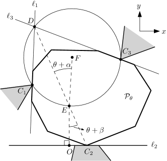
Figure 14: $\mathcal{P}_{\theta}$ satisfies the contact pairs $C_{i}=(A_{i},B_{i})$ for $i=1,2,3$.

$(2,2)$-changes. Suppose that $C_{1}$ and $C_{3}$ are corner contact pairs and $C_{2}$ and $C_{4}$ are side contact pairs, and $\mathcal{P}_{\theta}$ satisfies $C_{1},C_{2}$, and $C_{3}$. Let $\ell_{1},\ell_{2},$ and $\ell_{3}$ be the lines through $B_{1},A_{2},$ and $B_{3}$, respectively, and let $D=\ell_{1}\cap\ell_{3}$. Let $F$ be the center of the circumcircle to triangle $A_{1}A_{3}D$, and let $E$ be the intersection of the circumcircle and $B_{2}D$, other than $D$. Let $O$ be the perpendicular foot of $E$ to $\ell_{2}$. Let $\theta+\alpha$ be the angle from $\overrightarrow{EF}$ to $\overrightarrow{ED}$ and $\theta+\beta$ be the angle from $\overrightarrow{EO}$ to $\overrightarrow{EB_{2}}$ counterclockwise. See Figure 14. Since the angle between $\overrightarrow{DA_{1}}$ and $\overrightarrow{DB_{2}}$ remains unchanged while $\theta$ increases, $E,F$ and $O$ remain unchanged. We have $\overrightarrow{B_{2}B_{4}}=\Phi_{s,\vartheta}\overrightarrow{B_{2}D}$ for some $s$ and $\vartheta$. We also have $\overrightarrow{OB_{4}}=\overrightarrow{OB_{2}}+\overrightarrow{B_{2}B_{4}}=\overrightarrow{OB_{2}}+\Phi_{s,\vartheta}\overrightarrow{B_{2}D}=(|EO|\tan(\theta+\beta),0)+\Phi_{s,\vartheta}(-|EO|\tan(\theta+\beta)-2|EF|\cos(\theta+\alpha)\sin(\theta+\beta),|EO|+2|EF|\cos(\theta+\alpha)\cos(\theta+\beta))$. Observe that each point $V$ on segment $A_{4}$ can be parametrized to $\overrightarrow{OV}=s\vec{v}+\vec{c}$ for some $\vec{v}$ and $\vec{c}$. If $B_{4}$ touches $A_{4}$, then $s\vec{v}+\vec{c}=\overrightarrow{OB_{4}}$ is satisfied for some $s$. Thus, we obtain two equations for $\theta$ and $s$ in $x$- and $y$-coordinates. By eliminating $s$ using these two equations, we obtain the equation for $\theta$. By substituting $t=\tan{\frac{\theta+\beta}{2}}$, we obtain a quartic equation for $t$ which has at most four solutions. Therefore, there are at most four critical orientations for a $(2,2)$-change.

References

- [1] Pankaj K Agarwal, Nina Amenta, and Micha Sharir. Largest placement of one convex polygon inside another. Discrete & Computational Geometry, 19(1):95–104, 1998.
- [2] Pankaj K Agarwal, Boris Aronov, and Micha Sharir. Motion planning for a convex polygon in a polygonal environment. Discrete & Computational Geometry, 22(2):201–221, 1999.
- [3] Mikhail J Atallah. Dynamic computational geometry. In Proceedings of the 24th Annual Symposium on Foundations of Computer Science (FOCS 1983), pages 92–99. IEEE, 1983.
- [4] Francis Avnaim and Jean Daniel Boissonnat. Polygon placement under translation and rotation. In Robert Cori and Martin Wirsing, editors, STACS 88, pages 322–333. Springer Berlin Heidelberg, 1988.
- [5] Sang Won Bae and Sang Duk Yoon. Empty squares in arbitrary orientation among points. In Proceedings of the 36th International Symposium on Computational Geometry (SoCG 2020). Schloss Dagstuhl-Leibniz-Zentrum für Informatik, 2020.
- [6] Bernard Chazelle. The polygon containment problem. In F.P. Preparata, editor, Advances in Computing Research, Vol I: Computational Geometry, pages 1–33. JAI Press Inc., 1983.
- [7] L Paul Chew and Klara Kedem. Placing the largest similar copy of a convex polygon among polygonal obstacles. In Proceedings of the 5th Annual Symposium on Computational Geometry (SoCG 1989), pages 167–173, 1989.
- [8] L Paul Chew and Klara Kedem. A convex polygon among polygonal obstacles: Placement and high-clearance motion. Computational Geometry, 3(2):59–89, 1993.
- [9] Harold Scott Macdonald Coxeter and Samuel L Greitzer. Geometry revisited, volume 19. The Mathematical Association of America, 1967.
- [10] Rudolf Fleischer, Kurt Mehlhorn, Günter Rote, Emo Welzl, and Chee Yap. Simultaneous inner and outer approximation of shapes. Algorithmica, 8(1):365, 1992.
- [11] Steven Fortune. A fast algorithm for polygon containment by translation. In Proceedings of the 12th International Colloquium on Automata, Languages, and Programming (ICALP 1985), pages 189–198. Springer, 1985.
- [12] Jacob E. Goodman, Joseph O’Rourke, and Csaba D. Tóth, editors. Handbook of Discrete and Computational Geometry. CRC Press LLC, 3rd edition, 2017.
- [13] Daniel P Huttenlocher, Klara Kedem, and Jon M Kleinberg. On dynamic Voronoi diagrams and the minimum Hausdorff distance for point sets under Euclidean motion in the plane. In Proceedings of the 8th Annual Symposium on Computational Geometry (SoCG 1992), pages 110–119, 1992.
- [14] Klara Kedem and Micha Sharir. An efficient motion-planning algorithm for a convex polygonal object in two-dimensional polygonal space. Discrete & Computational Geometry, 5:43–75, 1990.
- [15] Seungjun Lee, Taekang Eom, and Hee-Kap Ahn. Largest triangles in a polygon. arXiv preprint arXiv:2007.12330, 2020.
- [16] Daniel Leven and Micha Sharir. Planning a purely translational motion for a convex object in two-dimensional space using generalized voronoi diagrams. Discrete & Computational Geometry, 2:9–31, 1987.
- [17] Nimrod Megiddo. Applying parallel computation algorithms in the design of serial algorithms. Journal of the ACM, 30(4):852–865, 1983.
- [18] Colm Ó’Dúnlaing and Chee K Yap. A retraction method for planning the motion of a disc. Journal of Algorithms, 6(1):104–111, 1985.
- [19] Micha Sharir and Sivan Toledo. Extremal polygon containment problems. Computational Geometry, 4(2):99–118, 1994.
- [20] Endre Szemerédi. On a problem by davenport and schinzel. Acta Arithmetica, 25:213–224, 1974.
- [21] Sivan Toledo. Extremal polygon containment problems. In Proceedings of the 7th Annual Symposium on Computational Geometry (SoCG 1991), pages 176–185. ACM, 1991.