First approximation for spacecraft motion relative to (99942) Apophis

S. Aljbaae^1,*, D. M. Sanchez¹, A. F. B. A. Prado¹, J. Souchay², M. O. Terra³, R. B. Negri¹, L. O. Marchi¹

1 Division of Space Mechanics and Control, INPE, C.P. 515, 12227-310 São José dos Campos, SP, Brazil.
2 SYRTE, Observatoire de Paris, PSL Research University, CNRS, Sorbonne Universités, UPMC Univ. Paris 06, LNE, 61 avenue de l’Observatoire, 75014 Paris, France.
3 Instituto Tecnológico de Aeronáutica, São José Campos, SP, 12228-900, Brazil.

* safwan.aljbaae@gmail.com

Abstract

We aim at providing a preliminary approach on the dynamics of a spacecraft in orbit about the asteroid (99942) Apophis during its Earth close approach. The physical properties from the polyhedral shape of the target are derived assigning each tetrahedron to a point mass in its center. That considerably reduces the computation processing time compared to previous methods to evaluate the gravitational potential. The surfaces of section close to Apophis are build considering or not the gravitational perturbations of the Sun, the planets, and the SRP. The Earth is the one that most affects the invisticated region making the vast majority of the orbits to collide or escape from the system. Moreover, from numerical analysis of orbits started on March 1, 2029, the less perturbed region is characterized by the variation of the semimajor axis of 40-days orbits, which do not exceed 2 km very close to the central body ($a<4$ km, $e<0.4$). However, no regions investigated could be a possible option for inserting a spacecraft into natural orbits around Apophis during the close approach with our planet. Finally, to solve the stabilization problem in the system, we apply a robust path following control law to control the orbital geometry of a spacecraft. At last, we present an example of successful operation of our orbit control with a total $\bigtriangleup v$ of 0.495 m/s for 60 days. All our results are gathered in the CPM-ASTEROID database, which will be regularly updated by considering other asteroids.
Key words: Celestial mechanics — minor planets, asteroids: individual (Apophis) — gravitation.

1 Introduction

The asteroid (99942) Apophis was discovered 16 years ago, on June 13th. 2004 (Smalley et al. (2005), cf. MPEC 2004-Y25). Soon after this discovery, its orbit was a particular subject of investigations. First simulations, badly constrained, lead to a hypothetic impact with the Earth in 2029, which although being quite improbable, could not be completely rejected. Then the hypothesis of impact with our planet was definitely rejected after more and more rigorous orbital simulations were carried out (Sansaturio and Arratia, 2008; Bancelin et al., 2012). Nowadays, after numerous refinements on the determination of initial conditions and orbital simulations, it is a well-established fact that (99942) Apophis will pass at a distance of $\sim$ 38,000 km, roughly six planetary radii, from the Earth’s center, on April 13${}^{\text{th}}$, 2029. Note that the asteroid will drive particular attention in the future, for other close encounters with our planet that are scheduled to occur in the XXI${}^{\text{th.}}$ centuty. In addition to the dramatic orbital changes caused by the 2029 close encounter with the Earth, complementary studies were oriented towards two objectives: first, the study of the Yarkovsky effect, which has to be taken into account for post-2029 refined orbital models (Bottke et al., 2006; Giorgini et al., 2008; Chesley et al., 2009); second, the modeling of important changes of rotational parameters, as the rotation rate and the orientation of the axis of rotation (Scheeres et al., 2005; Souchay et al., 2014, 2018).

In this paper we orientate our study towards an additional field of investigations: in a first step we determine the polyhedral shape and the gravity field of Apophis and, in a second step, we study the behavior of a test particle close to the asteroid, mainly perturbed by the gravitational action of the Earth and the Solar Radiation Pressure (referred as SRP hereafter) during the 2029 close encounter. In fact, Apophis appears to be in a state of non-principal axis rotation (tumbling). During the exceptional close approach, the tidal stresses and torques may cause resurfacing or reshaping of the body. However, this still a completely unknown interaction and very difficult to predict. As a preliminary step to propose a rendezvous mission to Apophis, we neglected the possible changes of the spin of the target and tried to approach a realistic analysis during the close approach. However, addressing this issue will be fundamental in future studies. In Sect. 2 we gather the necessary information to model the polyhedral shape of Apophis, from which we compute a 3D inertia tensor and calculate the spherical harmonic coefficients of the gravitational potential. Then, we construct a gravity model from which we can display the zero-gravity curves. In Sect. 3 we build the surfaces of section in a body-fixed frame. Sect. 4 concerns the specific case of the 2029 close encounter with the Earth, for which we model the modifications of the surfaces of section established in Sect.3 and by taking into account the SRP, we deduce the equations of motion of a test particle surrounding the asteroid, during the close approach. In Sect. 5, as an application of our inversions, we identify the less perturbed region around Apophis suitable to place a spacecraft around the asteroid. To compensate all the perturbations in the Apophis system, we apply orbital correction maneuvers in Sect. 6. Finally, a general presentation of our CPM-Asteroid (Close Proximity Motion relative to an Asteroid) database is presented in Sect. 7, which enables one to acquire insights into the orbital dynamics of a spacecraft near the asteroid (99942) Apophis.

2 Apophis shape model and Gravity field

To derive our model, we first describe some physical properties of Apophis, based in its polyhedral shape, considering an uniform density. We then consider a cloud of point masses (ideal spheres), which reproduces the total mass and moments of inertia of our target, as well as its gravitational field.

2.1 Physical Properties

Müller et al. (2014) observed Apophis with the Herschel Space Observatory Photodetector Array Camera and Spectrometer (PACS) instrument and classified our target as a Sq-class object most closely resembling LL ordinary chondrite meteorites. The author considered an Itokawa-like density ($\rho=1.75\pm 0.11$ g/cm³ (Lowry et al., 2014)) and estimated a mass ($M$) between $4.4$ and $6.2\times 10^{10}$ kg.

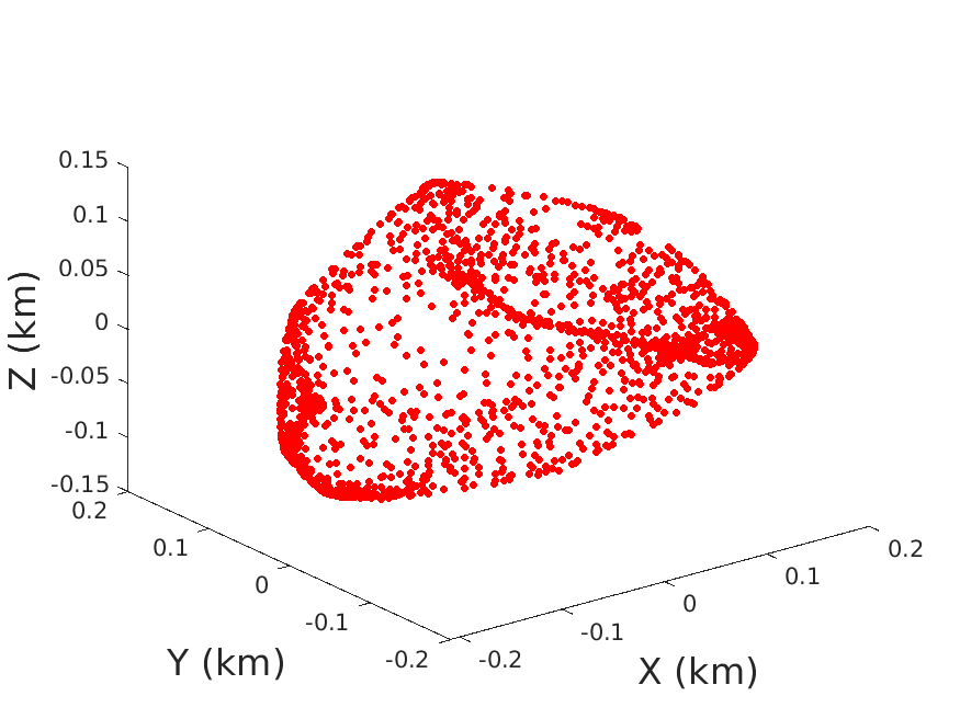
Our research focused on the real Apophis polyhedral shape obtained from extensive photometric observations by Pravec et al. (2014) and available in the 3D Asteroid Catalogue website. The authors showed that Apophis rotation is retrograde with a spin period of 30.4 h. According to Durech et al. (2010) and Hanuš et al. (2017), the photometry alone cannot provide information on asteroid sizes. Note that, concerning the asteroid (216) Kleopatra, Descamps et al. (2011) showed that, although its shape appears to be correct, the difference in the dimensions obtained from radar shape reconstruction and photometry can reach 20%. Moreover, Chanut et al. (2015b) found that the behavior of the zero velocity curves and the dynamics differ substantially if one applies a scale-size of 1.15 relative to the original shape of (216) Kleopatra. For that reason, we started our work by checking if the dimension of the reconstructed shape of Pravec et al. (2014) corresponds to the observed diameter (Müller et al., 2014). We determine the coefficient ($\gamma$), which links the volume of the polyhedral shape ($V$) with the mass ($M_{P}=V\rho$) to be compatible with the mass ($M$), when considering the Itokawa-like density ($\rho$). In other words, we choose suitable coefficients that multiply the coordinates x, y and z of the shape to find the polyhedral volume compatible with the mass and density estimated from the observation. Our results are presented in Table 1. Recently, Hanuš et al. (2017) presented shape models and volume for 40 asteroids from DAMIT shape modeling. The authors derived shape models and volumes for 41 asteroids using the ADAM algorithm from the inversion of their optical light curves, disk-integrated images from the Near-InfraRed Camera (Nirc2) at the Keck II telescope located at Maunakea in Hawaii and stellar occultation measurements. In this work, we just combined the volume with the mass estimation from the literature to derive the bulk density. We found a scale-size of $\gamma=0.285\pm 0.158$ relative to the polyhedral shape derived from Pravec et al. (2014), that must be applied to obtain a mass of $5.31\mp 0.9\times 10^{10}$ kg and a diameter of 0.387 km. Recently, Brozović et al. (2018) used the radar data to improve the shape of Pravec et al. (2014). The authors obtained a shape with 2000 vertices and 3996 faces. We also found a scale-size of 1.152 should be applied to obtain the mass and density already mentioned.

Table 1: The volume of (99942) Apophis with its correction coefficients relative to mass (2${}^{\text{nd}}$ column) and density (5${}^{\text{th}}$ column). The corrected diameter is displayed in the sixieme column.

Compatibility of Vol. with				Diameter	Diameter	shape
Mass		Density		(Original)	(Corrected)
Compatible	Coefficient	Compatible	Coefficient	km	km
NO	$0.285\mp 0.158$	NO	$0.285_{-0.0057}^{+0.0062}$	1.358	0.387	Pravec et al. (2014)
NO	$1.152\mp 0.638$	NO	$1.152_{-0.0232}^{+0.0252}$	0.336	0.387	Brozović et al. (2018)

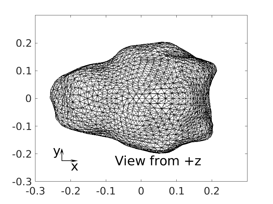
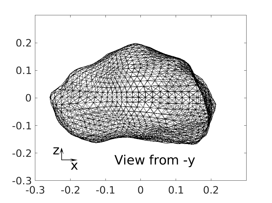
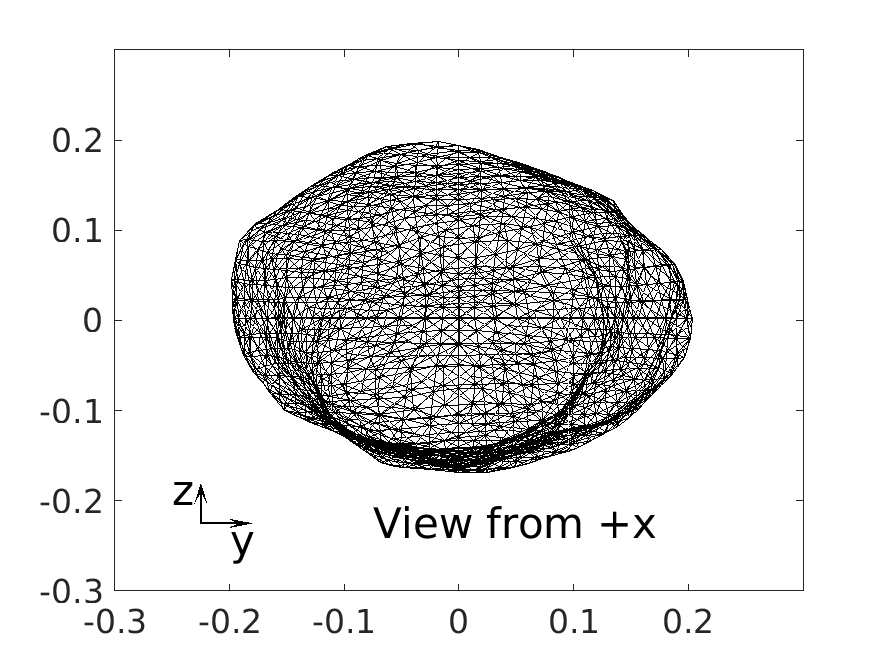
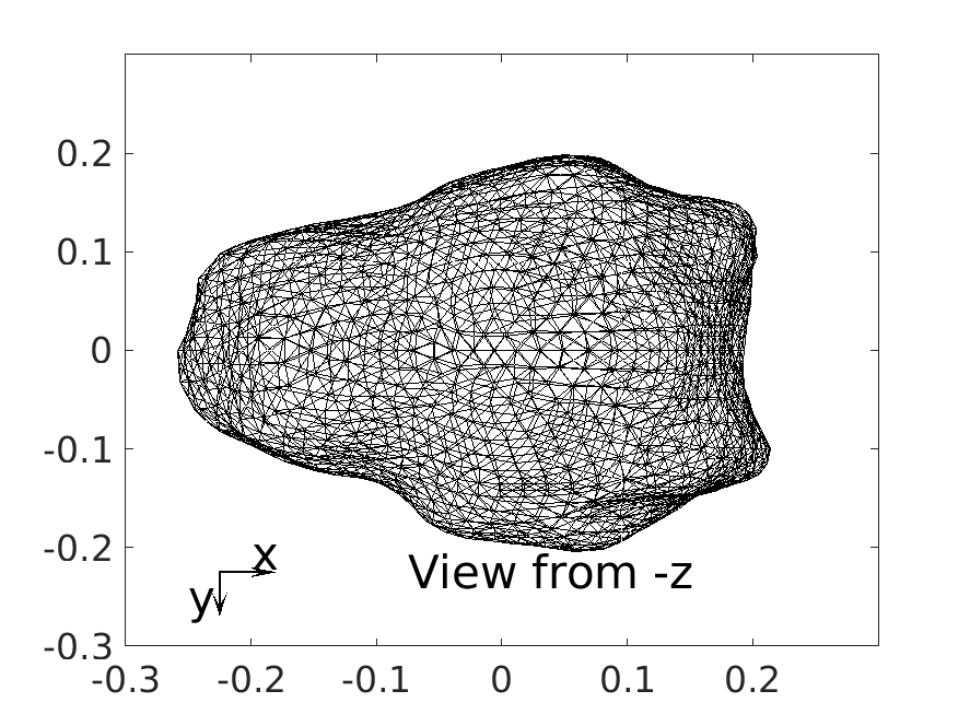
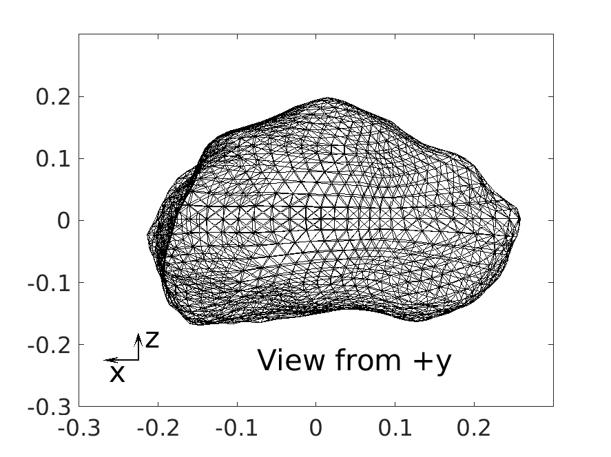
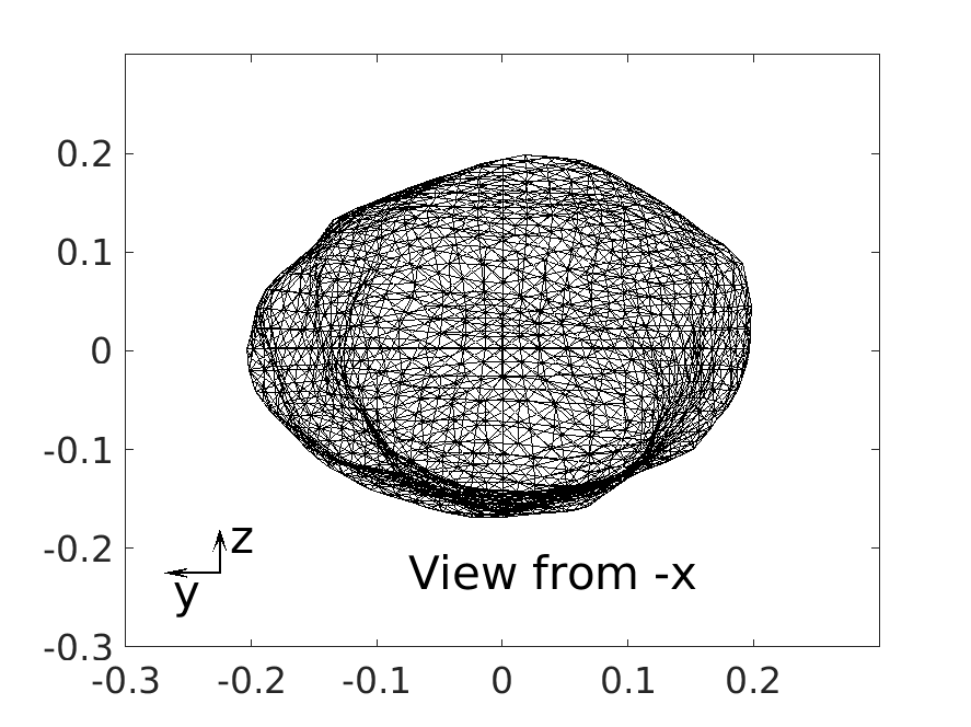
Using the algorithm of Mirtich (1996), we computed the 3D inertia tensor derived from each polyhedral shape of (99942) Apophis with a uniform Itokawa-like density. We found that this tensor is diagonal. This means that the body is perfectly oriented along its principal axes of inertia. The shape of our target is presented in Fig. 1. The overall dimensions of this shape are $(-0.280,0.259)\times(-0.184,0.191)\times(-0.156,0.169)$ km in the x-, y-, and z-directions, respectively, and the polyhedral volume is $0.03034285$ km³ (volume-equivalent diameter of 0.387 km).

The shape derived from Pravec et al. (2014): 1014 vertices and 2024 faces


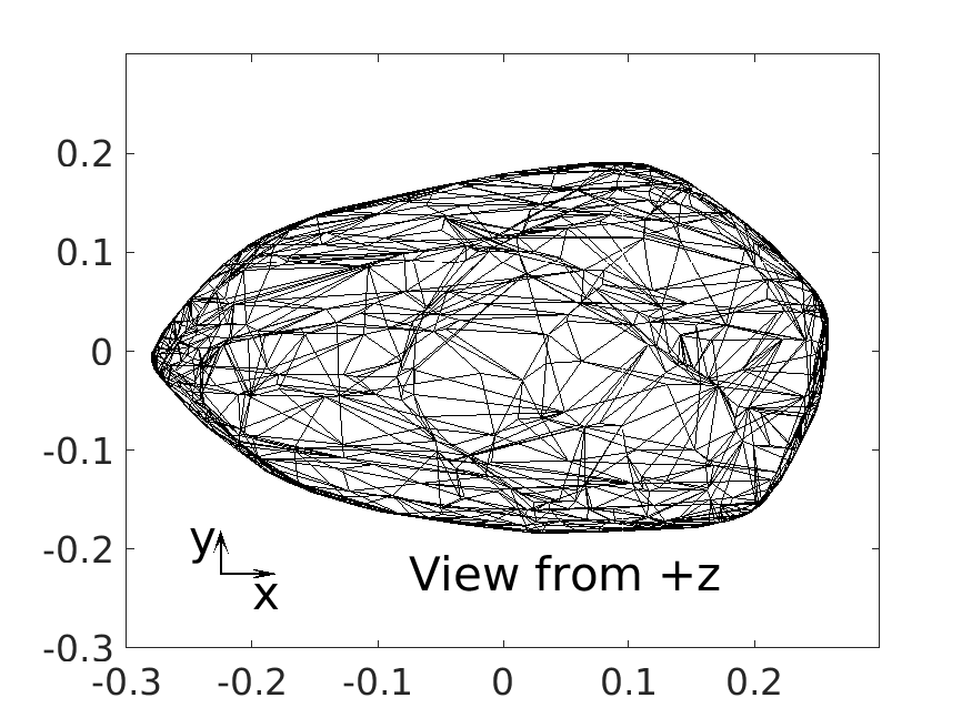
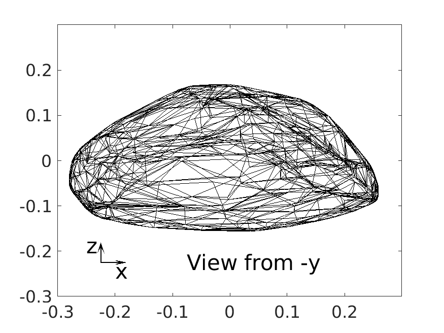
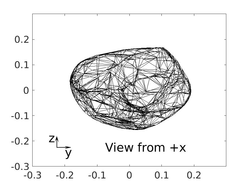
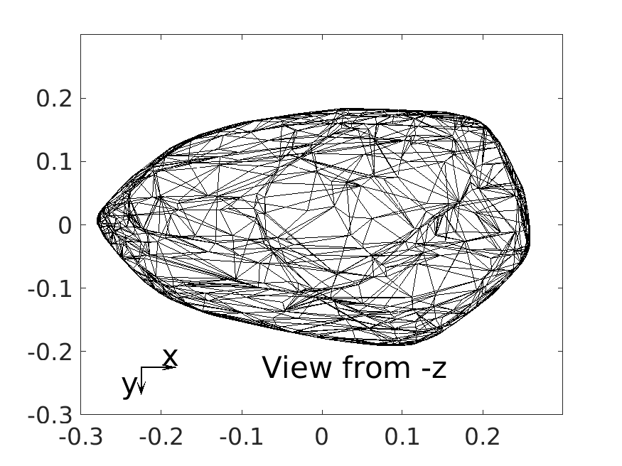
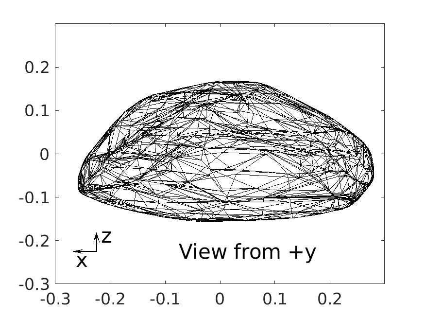
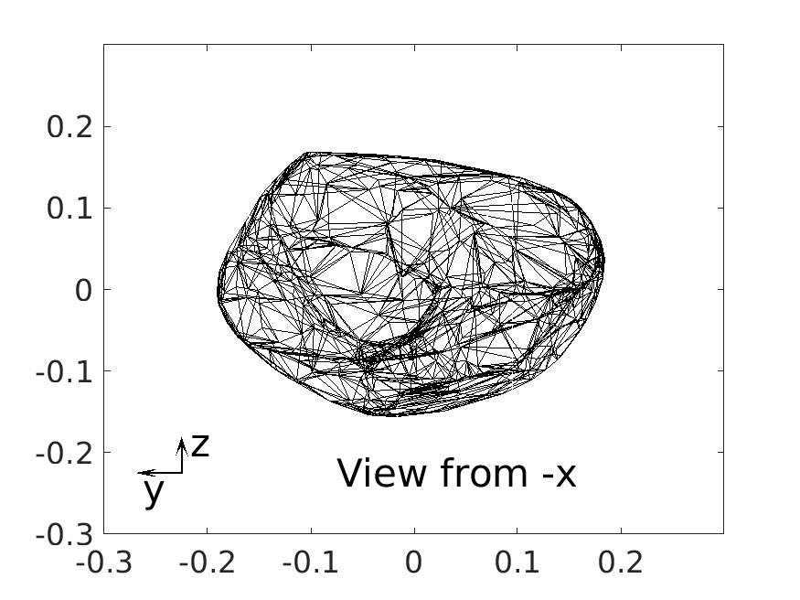
The shape derived from Brozović et al. (2018): 2000 vertices and 3996 faces

Figure 1: The polyhedral shape of (99942) Apophis shown in 6 perspective views ($\pm$ x, $\pm$ y, and $\pm$ z) after rescaling the shape with the reported volume-equivalent.

We then applied the algorithm of Werner (1997) to calculate the spherical harmonic coefficients $C_{n,m}$ and $S_{n,m}$ (up to degree 4, see Table 2). These coefficients are dimensionless, unnormalized parameters that describe the exterior gravitational potential $U$ of the body. They allow us to verify if the coordinate axes of the polyhedral shape are oriented with its principal axes of inertia. $C_{1,1}$ and $S_{1,1}$ should be zero if the expansion of the gravitational field is fixed around the center of mass; $C_{2,1}$, $S_{2,1}$ and $S_{2,2}$ should be zero if the axes are precisely oriented along the principal axes of inertia (Scheeres et al., 2000). However, we will not use these coefficients in our analyses. Our approach to calculating the exterior gravitational potential around the asteroid employs the polyhedral shape, that will be more accurate than the harmonic coefficients, even if these coefficients were measured up to a degree higher than four.

Table 2: Apophis Gravity Field Coefficients up to order 4, using 3996 triangular plates of the nonconvex shape model provided by Brozović et al. (2018). This coefficients are computed with the respect to a constant density of 1.75 $g.cm^{-3}$, a total mass of 5.310 $\times 10^{10}$ kg (derived from the polyhedron volume) and a reference distance of 0.193 km.

order	degree	$C_{nm}$	$S_{nm}$
0	0	1.0000000000	-
1	0	0.0000000000	-
1	1	0.0000000000	0.0000000000
2	0	-0.0783221323	-
2	1	0.0000000000	0.0000000000
2	2	0.0263789204	-0.0000000000
3	0	0.0448720700	-
3	1	0.0071441362	-0.0022479382
3	2	-0.0086800988	-0.0031712753
3	3	-0.0045154950	0.0001852096
4	0	0.0063633515	-
4	1	-0.0036166896	-0.0009014188
4	2	-0.0004122196	0.0002392422
4	3	0.0001533535	0.0002872799
4	4	0.0000804961	0.0000311549

2.2 The gravity model

Werner (1997) derived expressions to precisely evaluate the gravitational potential and acceleration components of a homogeneous polyhedron whose surface consists of a combination of planar triangles. Tsoulis and Petrović (2001) analyzed the singularities of the potential field caculated by the polyhedron. This method is considered as the best one to describe the gravitational field near or on the surface of a constant density polyhedron (Scheeres et al., 1998, 2000). Using the classical polyhedron method of Tsoulis and Petrović (2001), we compared the polyhedral shape derived from Pravec et al. (2014) and Brozović et al. (2018) in terms of the computational time and precision of orbit determination close to Apophis. A 60 days circular orbit with mechanical energy of $1.5\times 10^{-9}$ km²s${-2}$ at a distance of 1 km from the center the target could be integrated with 463 minutes using the shape of Pravec et al. (2014) and in 884 minutes using the shape of Brozović et al. (2018). The total variation distance of this orbit from the central body is 90.30 m in the first case and 88.60 m in the second one. In fact, the difference between the 2 shapes is inversely proportional to the distance from the center. Based on these results, taking into consideration the fact that we did not investigate collisions with Apophis, we think that using the shape of Pravec et al. (2014) with 1014 vertices and 2024 faces is a reasonable approach for the suit of this preliminary study, noting the difference in the execution time. Yet, the main problem of the classical polyhedral approach is the large computational effort, depending on the number of triangular faces chosen. This issue has been reported in Chanut et al. (2015a) and Aljbaae et al. (2017) applying the mascon gravity framework using a shaped polyhedral source, dividing each tetrahedron into several parts (Venditti, 2013). Inspired by this last idea, we first calculated the mass of each tetrahedron of the Apophis shape and assigned it to a point mass in the center of the tetrahedron. Thus, we considered the asteroid as a sum of 2024 points that correspond to the number of faces in the shape (Fig. 2).

Figure 2: Representation of (99942) Apophis modeled by a cloud of 2024 point masses.

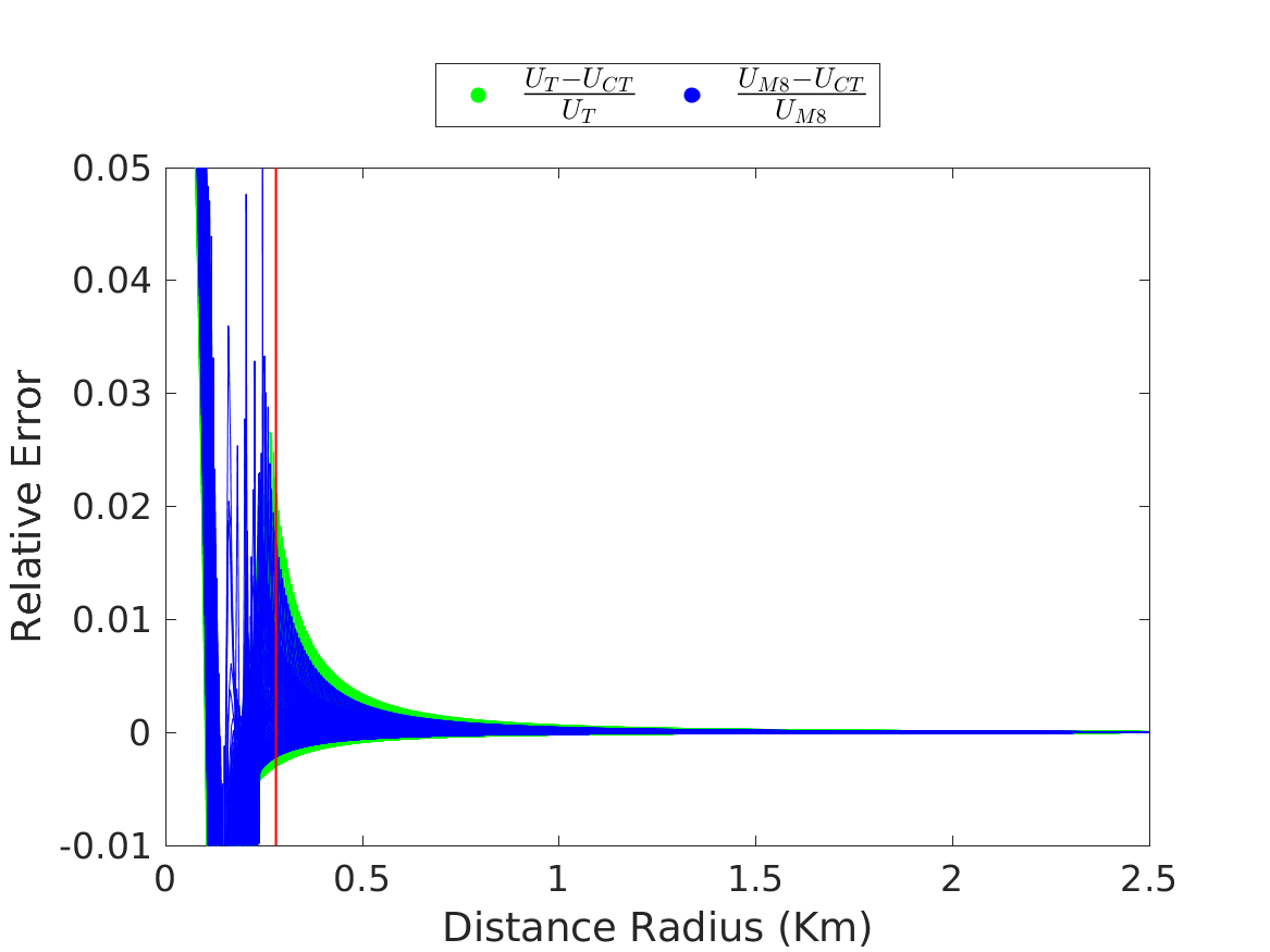
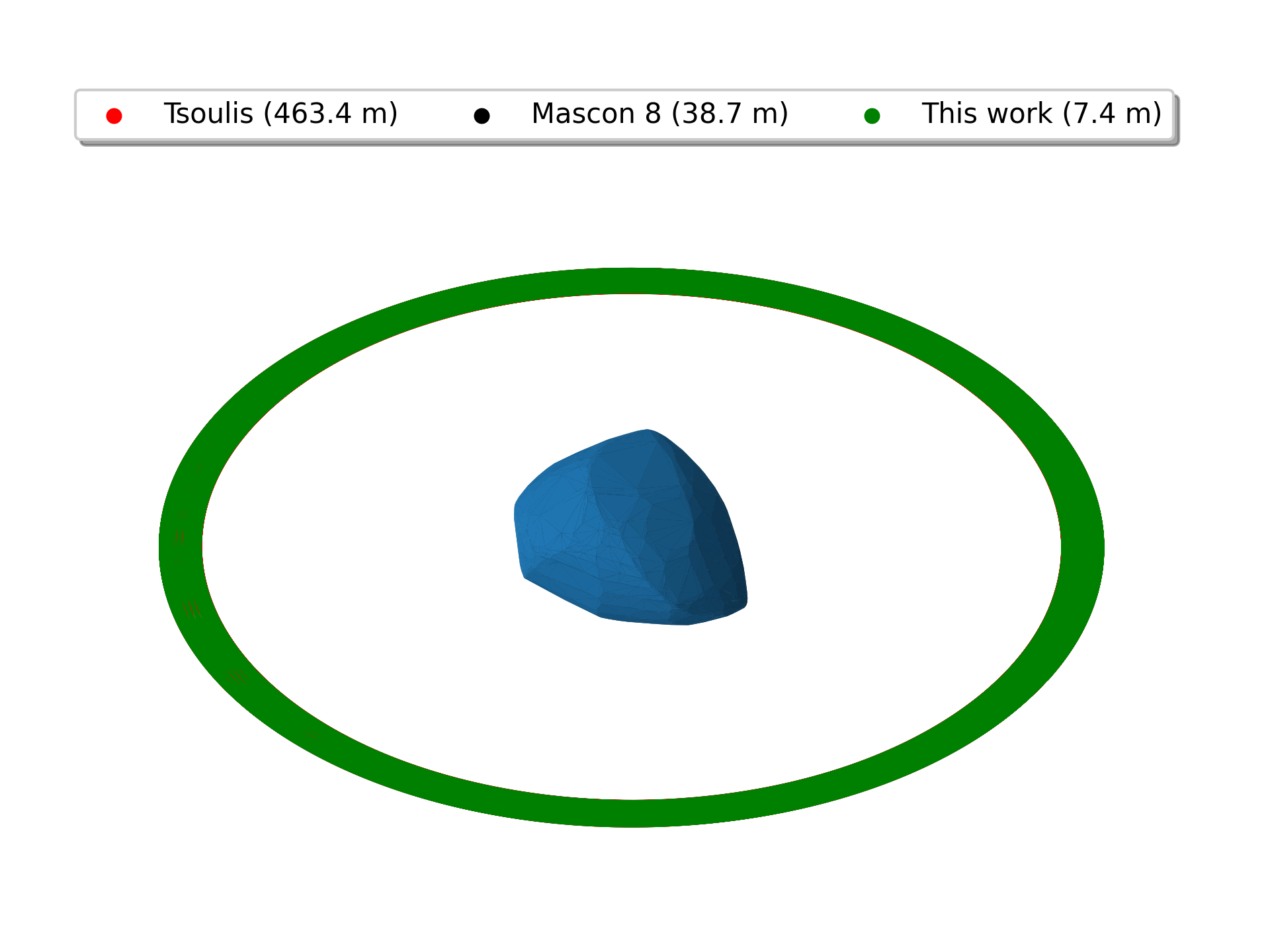
To show the efficiency of the method presented here to calculate the gravitational potential, we performed a series of tests comparing the potential, $U_{CT}$, calculated by our method (considering the asteroid as a sum of 2024 points in the center of the tetrahedron) with the classical polyhedron method, $U_{T}$, Tsoulis and Petrović (2001) and the Mascon gravity approach, dividing the asteroid into 8 layers, $U_{M8}$, Chanut et al. (2017); Aljbaae et al. (2017). In the top panel of Fig. 3, we present the relative errors between $U_{CT}$ and $U_{T}$ or $U_{M8}$, which show that our results are in good agreement with these models outside the body (right side of the red line). In the bottom panel of Fig. 3, we present three circular orbits around Apophis with the same initial conditions integrated using the three methods. The total variation distance from the central body, in each case, are presented in Table 5. In fact, we tried, in this work, to approach a realistic suite of simulations for motion about Apophis considering the real positions of the planets in our Solar System. To reach the minimum distance Earth-Apophis provided by the JPL’s HORIZONS ephemerides, we considered a step-size of 30 seconds in our integration, that makes the use of the classical polyhedron method very heavy in terms of the execution time, as shown in Table 5. Even with this small step of integration our introduction of the gravitational potential modeling considerably reduced the processing time keeping the accuracy at satisfactory levels.

Figure 3: Top: Relative error of the gravitational potential considering the asteroid as a sum of 2024 points in the center of the tetrahedron ($U_{CT}$) with the classical polyhedron method ($U_{T}$) or the model Mascon 8 ($U_{M8}$). Bottom: Three circular orbits around Apophis with the same initial conditions integrated using three methods. The execution time of each orbit is shown in parentheses in the legend

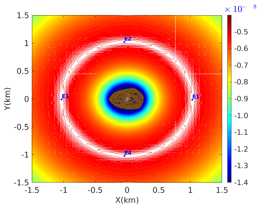
As we already mentioned, Apophis is a tumbling asteroid, by consequence, there are no equilibrium points in the real problem. However, in order to ensure that our model has no deadlocks, we use the three already mentioned above methods to calculate the Zero-velocity curves, neglecting the tumbling state of the target and the existence of other celestial bodies. Generaly speaking, the geometry of these curves has important implications for the stability of the trajectories around the asteroid (Yu and Baoyin, 2012). In Figs. 4 and 5 we present our results considering the asteroid as a sum of 2024 points (one point in the center of each tetrahedron). We identified four equilibrium points, two points along the x-axis and two points along the y-axis. The locations of the equilibrium points and the errors (%) with respect to the classical polyhedron method (Tsoulis and Petrović, 2001) are listed in Table 3.

Figure 4: Zero-velocity surfaces in Apophis equatorial plane (z = 0) assuming a uniformly rotating 2024 points gravity field.

Figure 5: Zero-velocity surfaces around Apophis with different values of the Jacobi constant.

Table 3: Locations of the 4 equilibrium points of (99942) Apophis, with the relative errors (%) with respect to the classical polyhedron method (Tsoulis and Petrovic, 2001) and the value of the Jacobi constant C (using the shape model with 1014 vertices and 2024 faces).

	x (km)	y (km)	z (km)	Errors (%)	$C(km^{2}s^{-2}$)
Tsoulis and Petrovic
$E_{1}$	1.031511633	-0.015403571	-0.001193548		-0.521305965 $\times 10^{-8}$
$E_{2}$	-0.047314147	1.020569106	0.000543576		-0.517908205 $\times 10^{-8}$
$E_{3}$	-1.032399019	-0.008968726	-0.001245442		-0.521512451 $\times 10^{-8}$
$E_{4}$	-0.044140503	-1.020703353	0.000489828		-0.517905804 $\times 10^{-8}$
Chanut et al. (2015a); Aljbaae et al. (2017)
$E_{1}$	1.031356216	-0.015946043	-0.001144834	0.01427	-0.521254519 $\times 10^{-8}$
$E_{2}$	-0.045642642	1.020709220	0.000513721	0.00625	-0.517929162 $\times 10^{-8}$
$E_{3}$	-1.031250000	-0.044075355	-0.001210880	0.02388	-0.521445551 $\times 10^{-8}$
$E_{4}$	-0.043612570	-1.020784265	0.000466467	0.00569	-0.517925320 $\times 10^{-8}$
This work
$E_{1}$	1.031020908	-0.014074537	-0.000975681	0.04942	-0.521130609 $\times 10^{-8}$
$E_{2}$	-0.041280470	1.021029506	0.000441225	0.01941	-0.517974994 $\times 10^{-8}$
$E_{3}$	-1.031741294	-0.007887703	-0.001003436	0.06458	-0.521297563 $\times 10^{-8}$
$E_{4}$	-0.039861524	-1.021073280	0.000403140	0.01895	-0.517971558 $\times 10^{-8}$

We also examined the stability of the equilibrium points by calculating the eigenvalues of the linearized system (Table 4). We found three pairs of purely imaginary eigenvalues for $E_{2}$ and $E_{4}$ points, showing that these solutions are linear stable with the linearized vector field exhibiting a behavior of the kind center x center x center. On the other hand, the linear analysis reveals that $E_{1}$ and $E_{3}$ points are unstable equilibria of the kind center x center x saddle, given that we obtained one pair of real eigenvalues with opposite signals and two pairs of purely imaginary eigenvalues for this case. Therefore, according to the classification proposed by Jiang et al. (2014) and Wang et al. (2014), these solutions belong to Case 1 and 2, respectively. Moreover, our target can be classified as a type-I asteroid, according to the classification proposed by Scheeres (1994).

Table 4: Eigenvalues of the coefficient matrix of the 4 external equilibrium points.

eigenvalues	$E_{1}$	$E_{2}$	$E_{3}$	$E_{4}$
	$\times 10^{-4}$	$10^{\times-4}$	$10^{\times-4}$	$\times 10^{-4}$
Tsoulis and Petrović (2001)
$\lambda_{1}$	+0.5826 $i$	+0.5752 $i$	+0.5862 $i$	+0.5755 $i$
$\lambda_{2}$	-0.5826 $i$	-0.5752 $i$	-0.5862 $i$	-0.5755 $i$
$\lambda_{3}$	+0.5805 $i$	+0.5547 $i$	+0.5813 $i$	+0.5535 $i$
$\lambda_{4}$	-0.5805 $i$	-0.5547 $i$	-0.5813 $i$	-0.5535 $i$
$\lambda_{5}$	-0.1314	+0.1438 $i$	-0.1497	+0.1473 $i$
$\lambda_{6}$	+0.1314	-0.1438 $i$	+0.1497	-0.1473 $i$
Chanut et al. (2015a); Aljbaae et al. (2017)
$\lambda_{1}$	+0.5805 $i$	+0.5749 $i$	+0.5812 $i$	+0.5749 $i$
$\lambda_{2}$	-0.5805 $i$	-0.5749 $i$	-0.5812 $i$	-0.5749 $i$
$\lambda_{3}$	+0.4709 $i$	+0.3662 $i$	+0.4744 $i$	+0.3671 $i$
$\lambda_{4}$	-0.4709 $i$	-0.3662 $i$	-0.4744 $i$	-0.3671 $i$
$\lambda_{5}$	-0.1727	+0.2571 $i$	-0.1822	+0.2559 $i$
$\lambda_{6}$	+0.1727	-0.2571 $i$	+0.1822	-0.2559 $i$
This work
$\lambda_{1}$	+0.5821 $i$	+0.5752 $i$	+0.5851 $i$	+0.5754 $i$
$\lambda_{2}$	-0.5821 $i$	-0.5752 $i$	-0.5851 $i$	-0.5754 $i$
$\lambda_{3}$	+0.5802 $i$	+0.5561 $i$	+0.5807 $i$	+0.5551 $i$
$\lambda_{4}$	-0.5802 $i$	-0.5561 $i$	-0.5807 $i$	-0.5551 $i$
$\lambda_{5}$	-0.1272	+0.1384 $i$	-0.1426	+0.1416 $i$
$\lambda_{6}$	+0.1272	-0.1384 $i$	+0.1426	-0.1416 $i$

Finally, It is important to recall that, in terms of the execution time on computers Pentium 3.60GHz, our model reduced the computation processing time by more than 95% compared to the classical polyhedron method, losing less than 2% of the precision in the tested area (Table 5). However, this point will be much more important if we need integration for larger times. That motivated us to represent our target as a cloud of 2024 point masses for the rest of this work.

Table 5: CPU execution time to caculate the potential around (99942) Apophis, using a Pentium 3.60GHz computers.

	Tsoulis	Mascon 8	This work
1,002,000 points	65m27.337s	8m9.347s	0m18.337s
60 days orbit	463m24.751s	38m39.966s	7m21.495s
grey80$\bigtriangleup r$ (m)	90.30	90.05	89.50

3 Surfaces of Section

In this section, we build the surfaces of section related to the potential of Apophis in the body-fixed frame. Our model is similar to that presented in Borderes-Motta and Winter (2018); Jiang et al. (2016). However, we use the mechanical energy of orbits around our target, as presented in Scheeres et al. (2000); Aljbaae et al. (2019)

$$H = \frac{1}{2}(\dot{x}^{2}+\dot{y}^{2}+\dot{z}^{2})-\frac{1}{2}\omega^{2}(x^{2}+y^{2})-U$$

$$U = +\sum_{i=1}^{2024}\frac{\mathcal{G}m_{i}}{r_{i}}$$

.
where: $x,y,z$ and $\dot{x},\dot{y},\dot{z}$ are the location and velocity of the particle in the body-fixed frame of reference. $U$ is the gravitational potential of the asteroid, calculated using one point fixed in the center of each tetrahedron, as explained in the previous section. $\mathcal{G}m_{i}$ is the gravitational parameter of the $i$th. tetrahedron, with $\mathcal{G}=6.6741\times 10^{-20}$ km³kg^-1s^-2. $r_{i}$ is the distance between the center of mass of the tetrahedron and the particle. The equatorial prograde motion of a massless particle around Apophis is determined numerically with the Runge-Kutta 7/8 integrator with variable step size, optimized for the accuracy of $10^{-12}$, covering a maximum of 200 years. We stop our integration after 3000 intersections between the trajectory and the plane $y=0$. However, this does not necessarily ensure that the nature of all orbits remains unchanged in time, because some orbits may manifest a nonlinear behavior as time goes on. We distributed our initial conditions in the y-axis, with $x_{0}=z_{0}=\dot{y}_{0}=\dot{z}_{0}=0$ and $\dot{x}_{0}$ was computed according to Eq. 3. The values of $y_{0}$ are taken between 0.5 and 10 km from the asteroid center with an interval of 0.1 km. We first consider our target significantly far from any other celestial body, where the motion is dominated by the asteroid own gravitational field. In this section, we also neglected the SRP. The equation of motion used in this analysis is as follows:

$$\ddot{\text{r}} = -2\Omega\times\dot{\text{r}}-\Omega\times(\Omega\times\text{r})+U_{\text{r}}$$

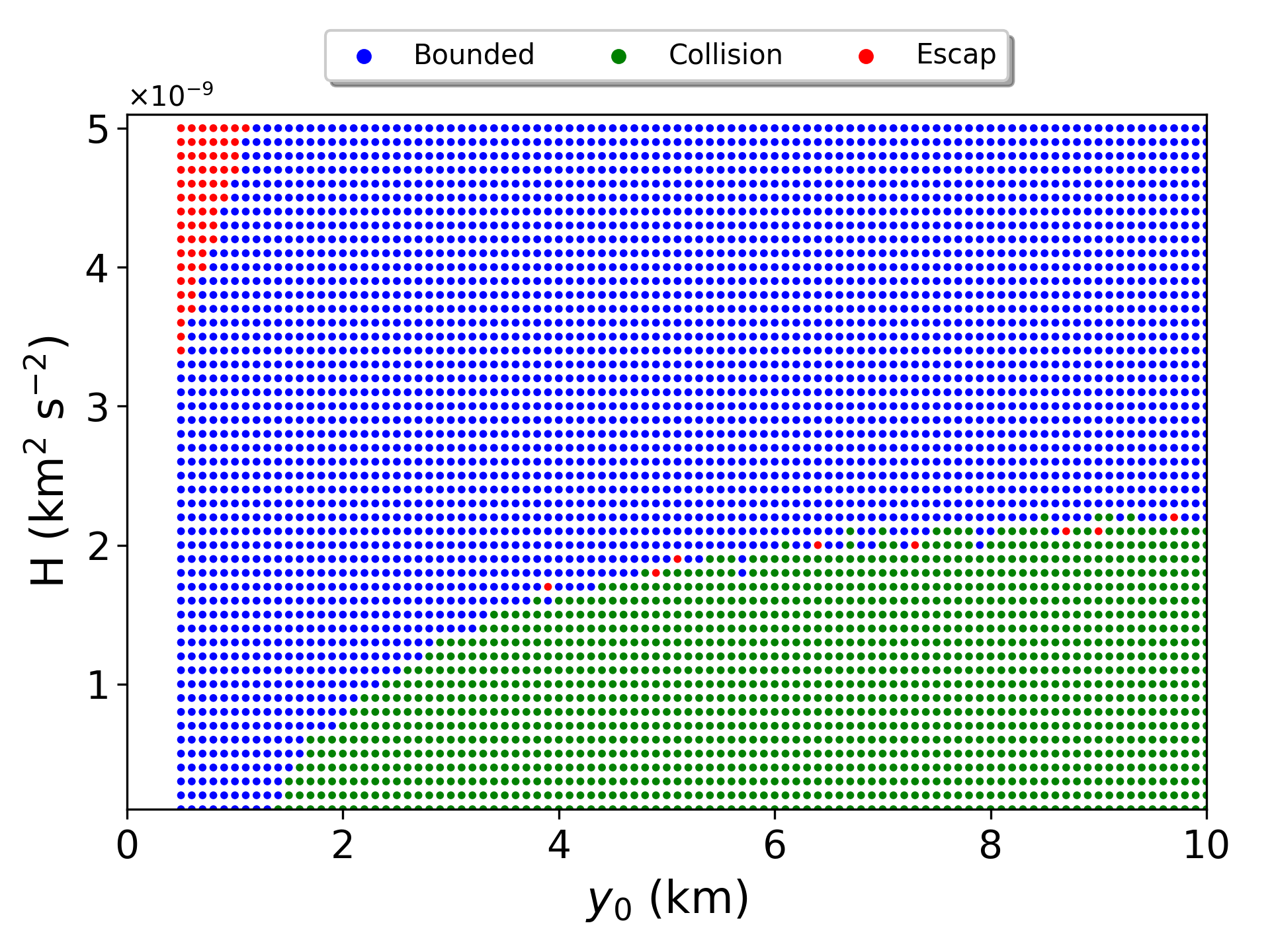
where r is the coordinate vector of the particle in the body-fixed frame, $\Omega$ is the rotation vector from the uniform rotation of (99942) Apophis, and $U_{\text{r}}$ is the gradient of the gravitational potential of the central body, calculated considering it as a sum of 2024 points (Sect. 2). In Fig. 6, we present the initial conditions that generate orbits escaping from the system (red points), colliding with the central body (green points), and bounded orbits around our target (blue points). The orbit escapes from Apophis system when the distance from the central body becomes 10 times greater than the Apophis Hill sphere (34 km). We considered a relatively high distance to be sure that the orbits beyond this limit will certainly not return back. The collision with the central body occurs when the particle crosses the limit of the polyhedral shape of Apophis using the Computational Geometry Algorithms Library (CGAL). We notice that, no collision with the central body occurs for $H>2.2\times 10^{-9}$. The escapes from the system occur for an initial $H>3.4\times 10^{-9}$ with some particles escaping with $1.7\times 10^{-9}\leq H\leq 2.2\times 10^{-9}$. In agreement with Aljbaae et al. (2019, 2020), the particles escape from Apophis system when they are very close to the central body and have sufficient energy.

Figure 6: Type of orbits around the asteroid (99942) Apophis. Neglecting the perturbations of the planets in our Solar System and the SRP.

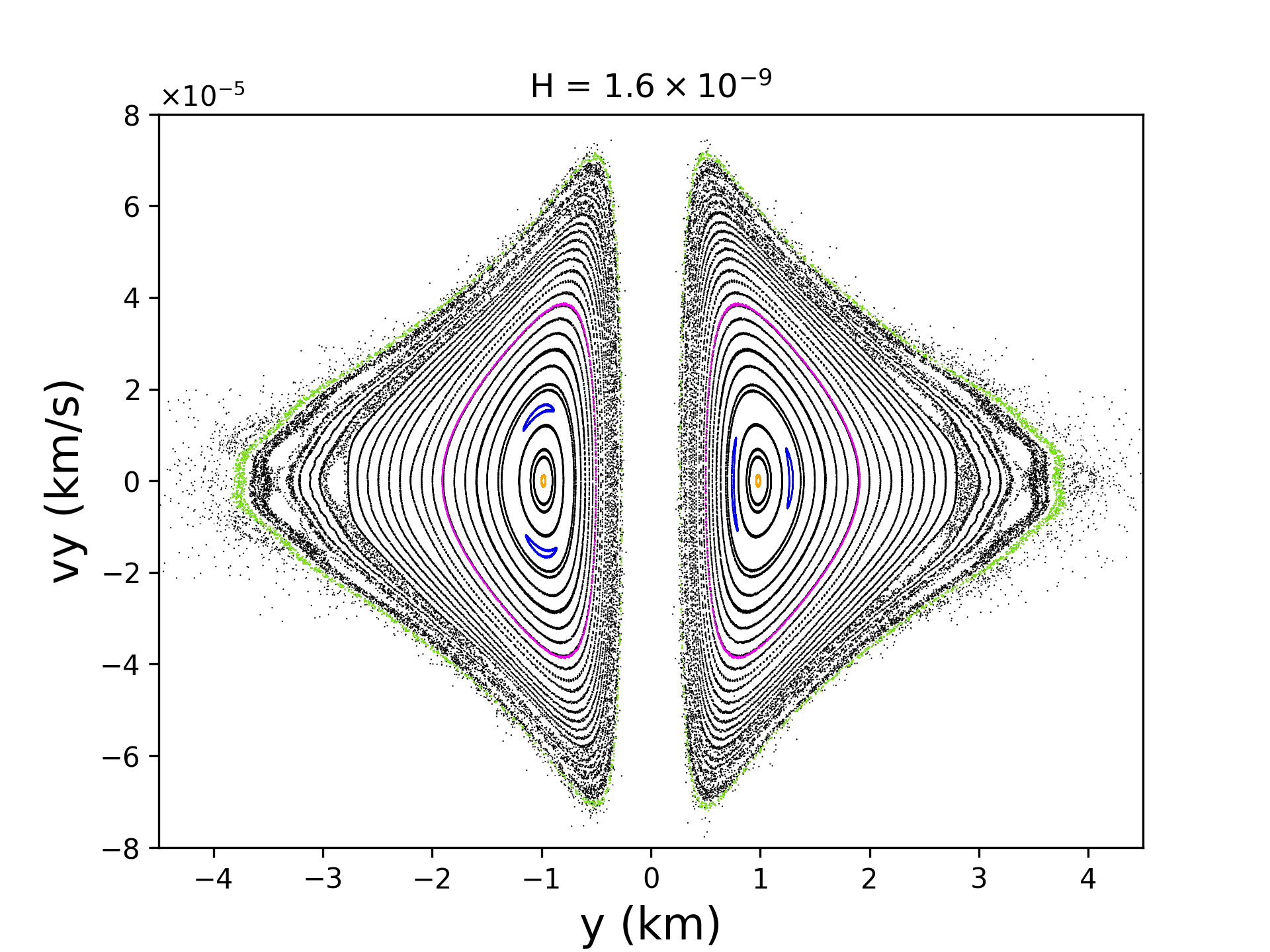
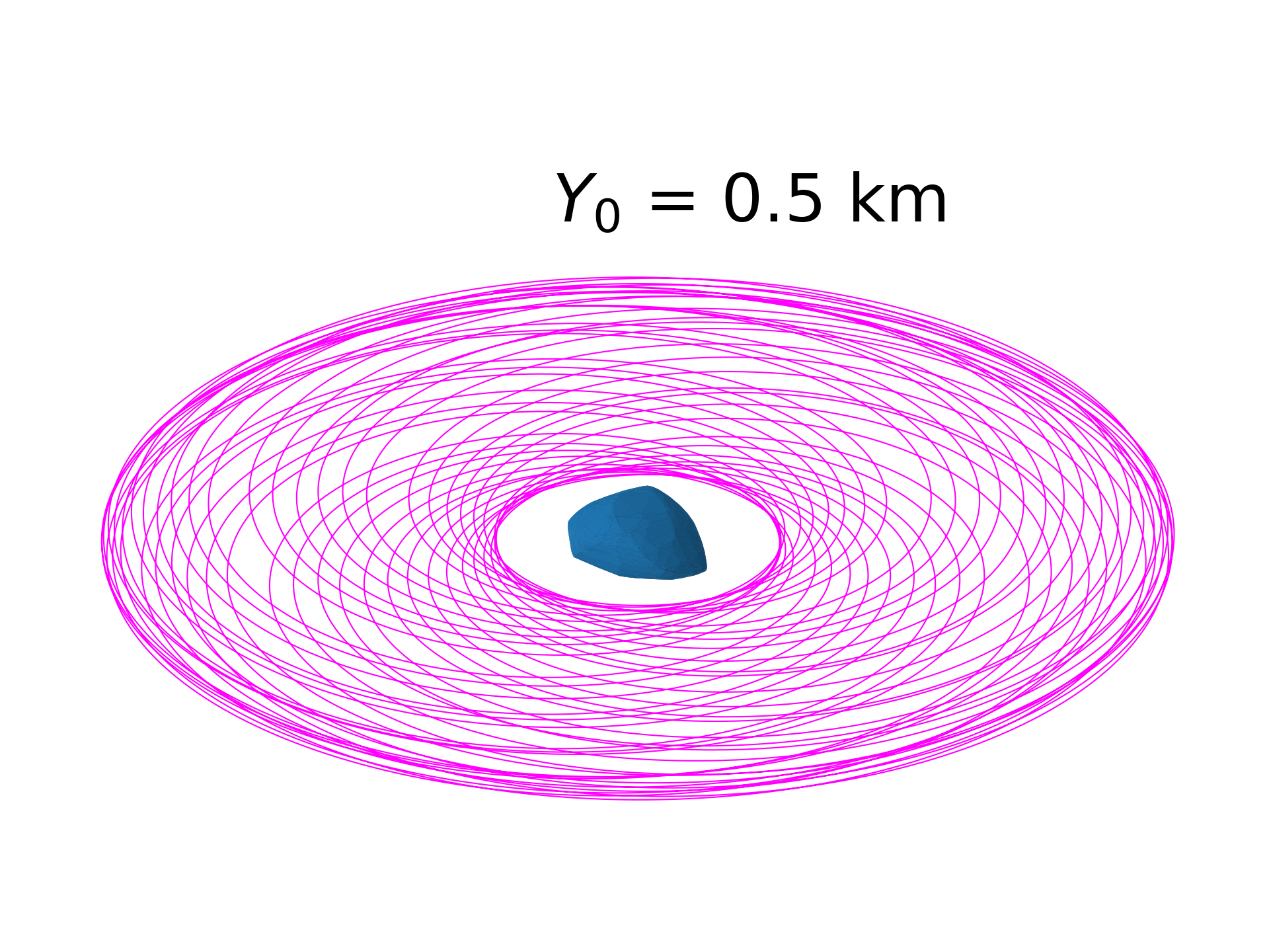
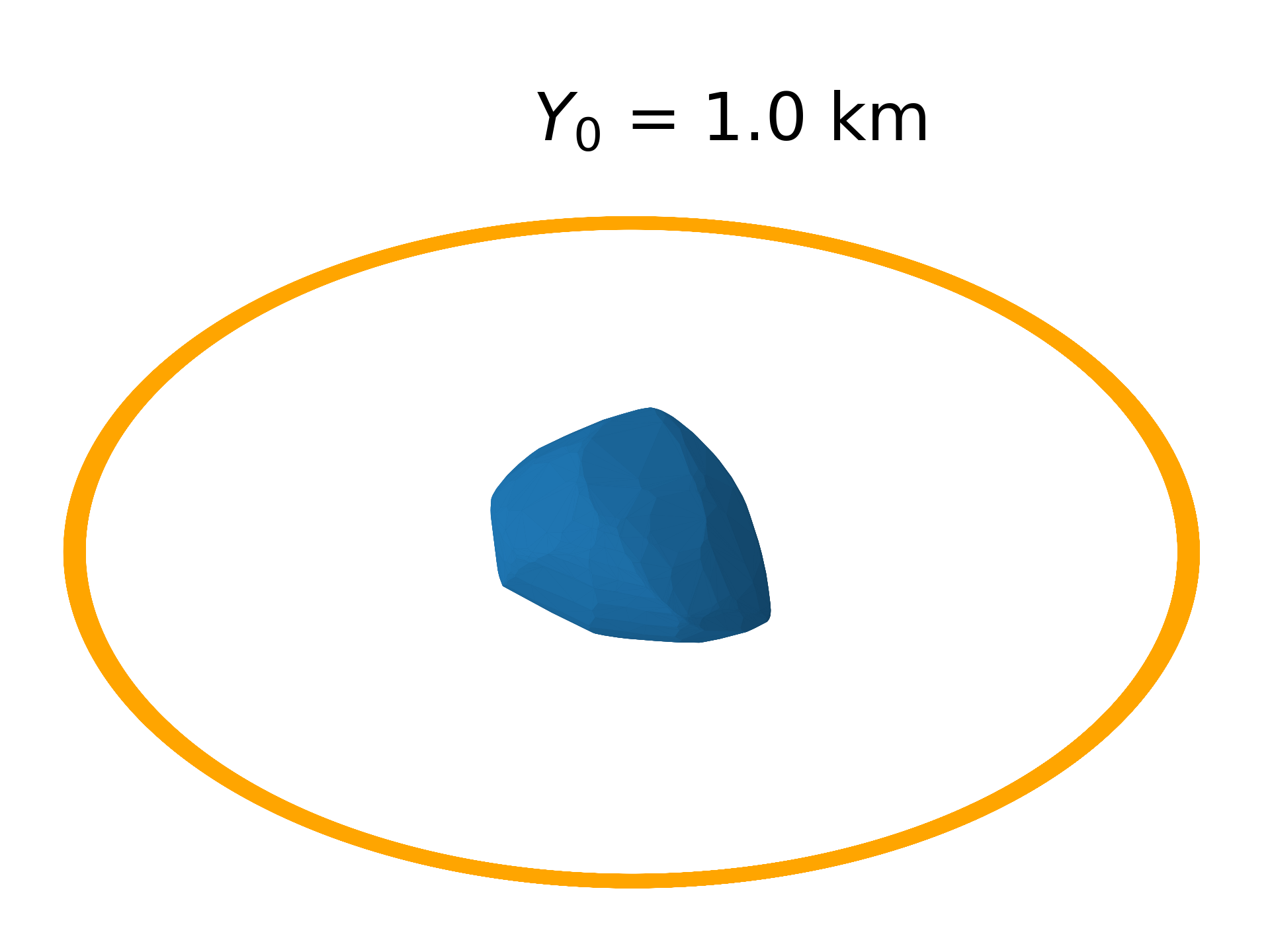
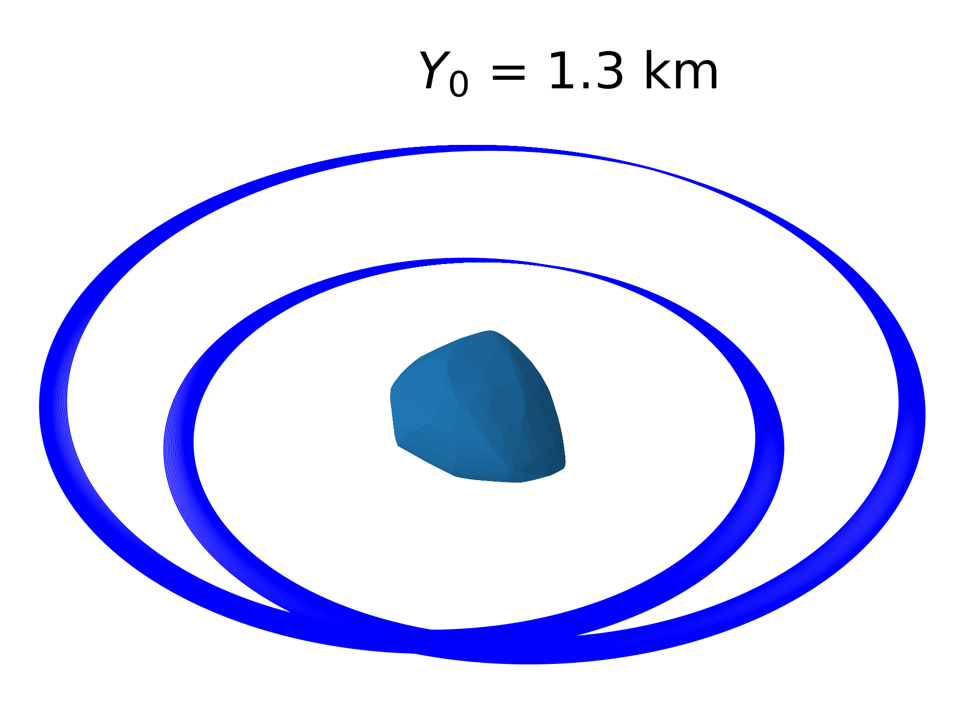
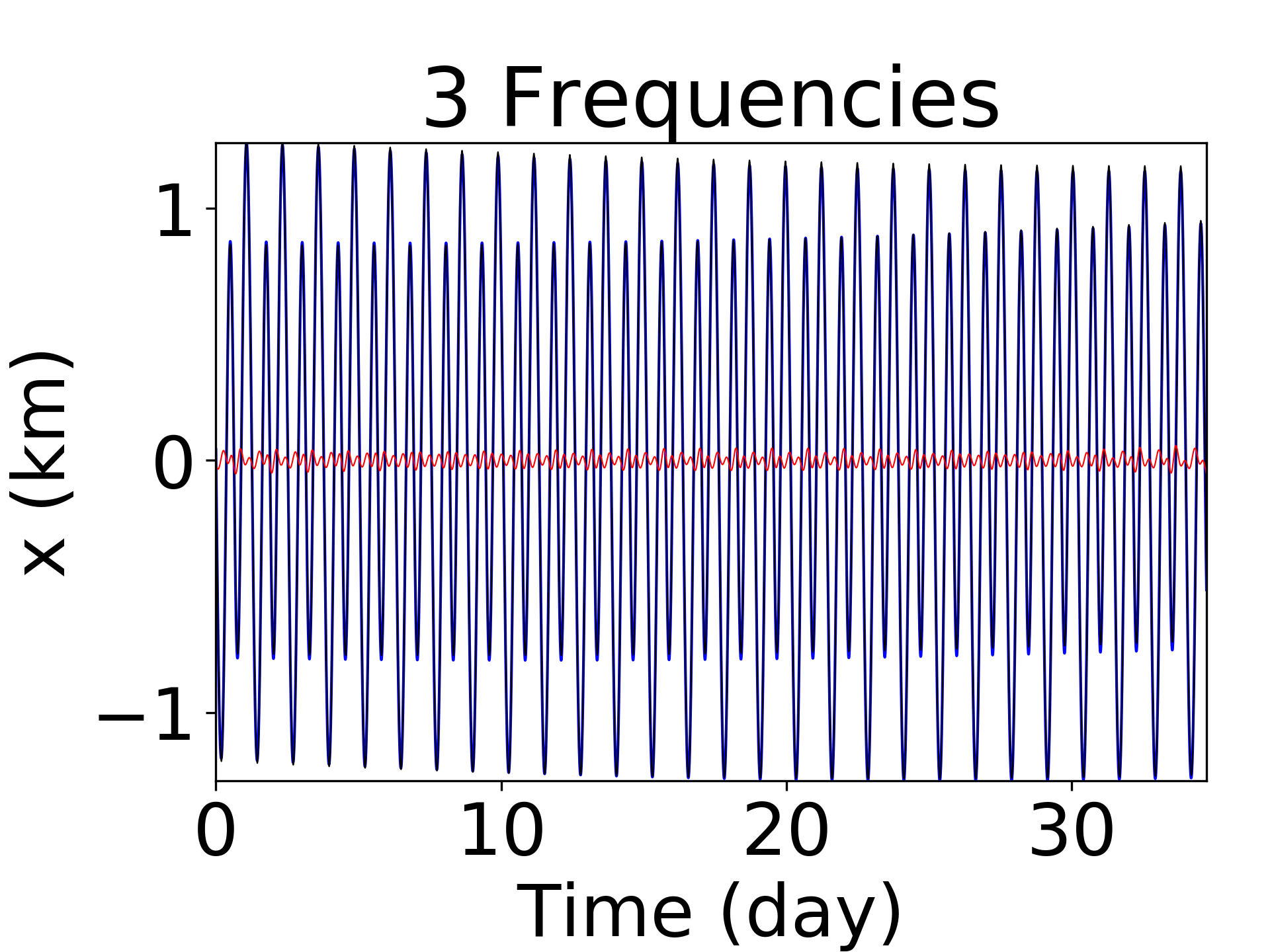
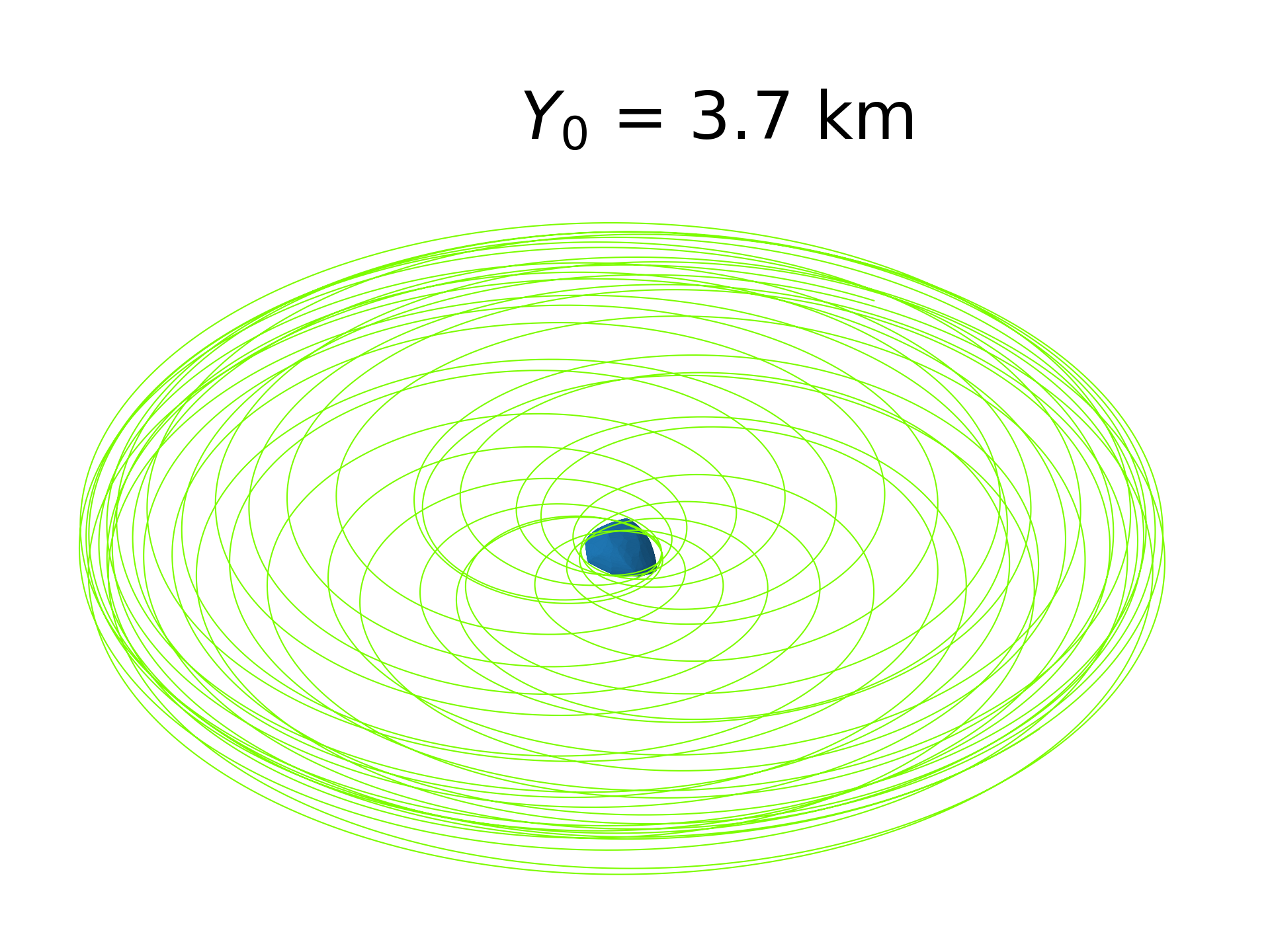
An example of our results for $H=1.6\times 10^{-9}$ is presented in Fig. 7. This plot gives quick overview of the orbital structure. We can easily distinguish between regular and chaotic motion. The isolated points, for instance, represent chaotic orbits, while areas with no points represent areas that are not reachable by any orbit. When we have one point in the Surface of Section, we get a periodic orbit, while a quasi-periodic motion is depicted by a closed curve. In fact, the period of an orbit is not defined by the Surface of Section itself, because the number of dots depend on which section is chosen. In Fig. 7, we also present some orbits in the Apophis system. To characterize the periodicity of these orbits, we perform a frequency analysis of the x, y, and z-coordinate of each orbit and determine the leading frequencies. For that purpose, we first evaluated and removed the quadratic variation of the coordinate of the form

$$\alpha+\beta t+\gamma t^{2}.$$

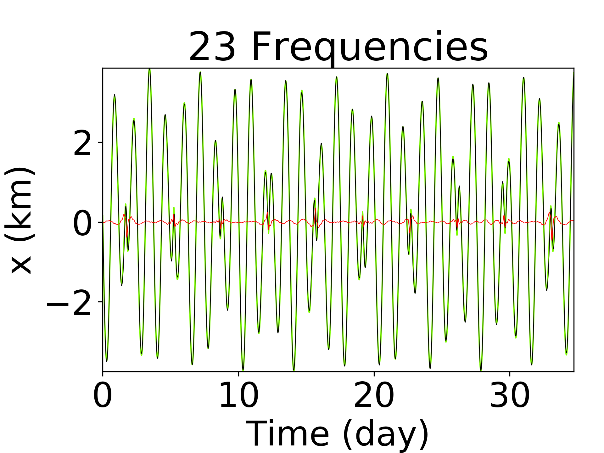
Then, we use the Fast Fourier Transform (FFT) to determine the leading frequencies. Our analysis is well adapted for dense polynomials using the software TRIP, developed at the IMCCE-Paris Observatory by Gastineau and Laskar (2011). For the sake of clarity and to limit the computational time cost, we restrict our analysis to the first 30 days of integration time. We find complex periods and amplitudes representing our signal. Finally, we fit a nonlinear regression approach to model our signal using the Least-Square method, following an expression combining Fourier-type and Poisson-type components in the form:

$$x(t)=\sum_{i=1}^{N} \bigg{[} A_{i}\sin(f_{i}t)+B_{i}\cos(f_{i}t)+$$

$$C_{i}t\sin(f_{i}t)+D_{i}t\cos(f_{i}t)\bigg{]}.$$

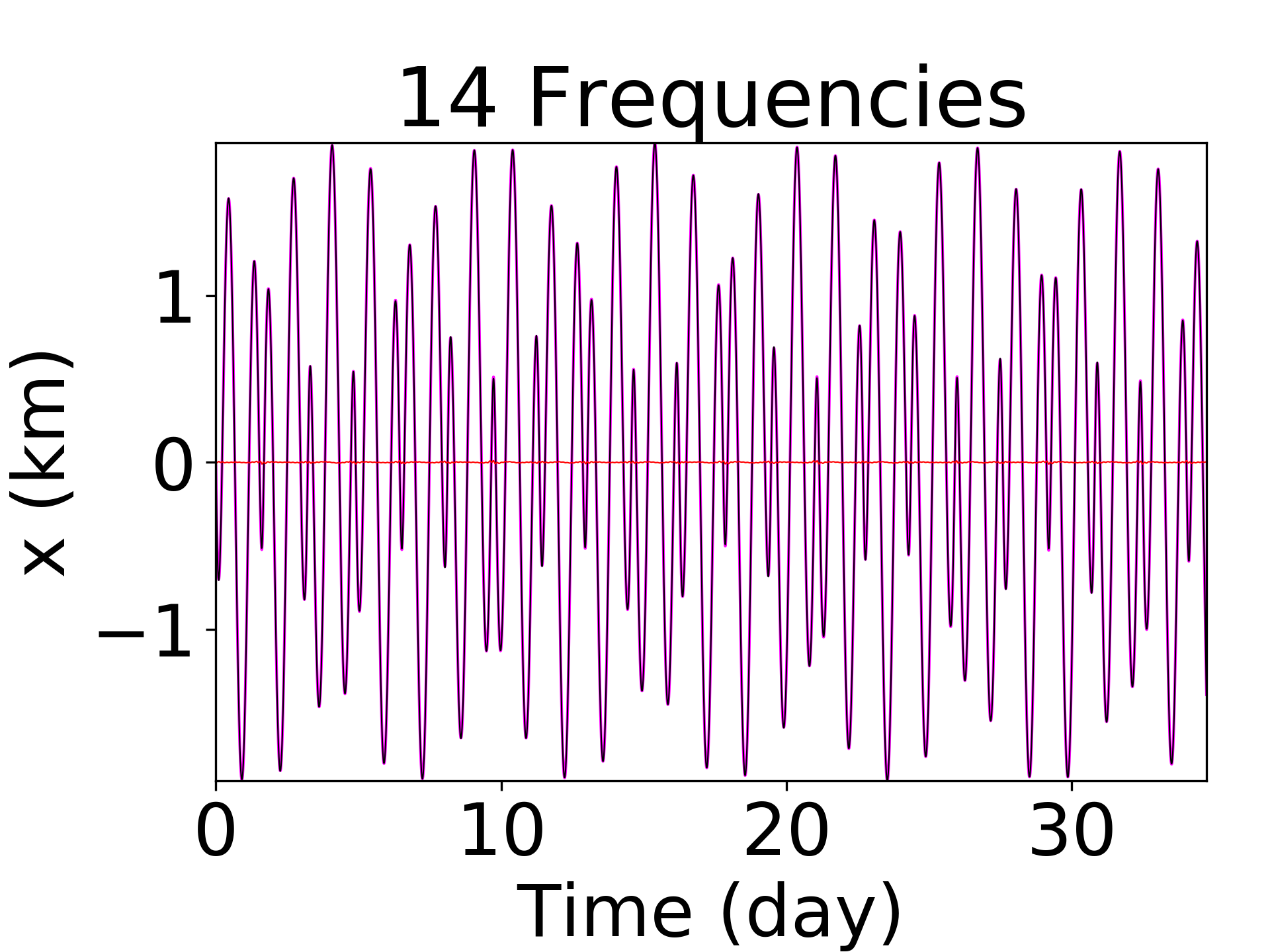
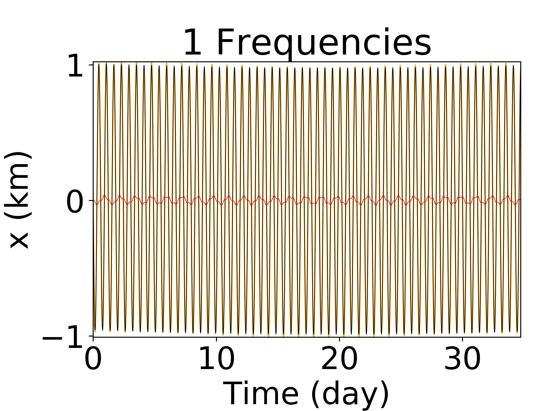
For the sake of simplicity and completeness, we present our results on the x-coordinate in the right-hand side of Fig. 7. We can observe a good quality of the fit resulting from the least-squares-analysis. The flat red curves represent the residuals obtained after subtracting a combination of the sinusoids (black curves) from the original signal. These sinusoids are listed in Table 6. For more details about our frequency analysis, the interested reader can refer to Aljbaae and Souchay (2012) and Aljbaae (2013). Overall, our frequency analysis perfectly determines the orbits around our target. Our results consist of different mechanical energy gathered in the CPM-Asteroid database (Close Proximity Motion relative to an Asteroid). Moreover, we include in this database the influence of close approach with our planet, witch is the subject of the next section.

Table 6: Coefficients of Fourier and Poisson series for the x-coordinate of some orbits.

$Y_{0}=0.5$ km
$\alpha$: -0.175134$\times 10^{-1}$         $\beta$: 0.371340$\times 10^{-2}$         $\gamma$:-0.132787$\times 10^{-3}$
Period (days)	$A_{i}\times 10^{-3}$	$B_{i}\times 10^{-7}$	$C_{i}\times 10^{-7}$	$D_{i}\times 10^{-7}$
5.005097	1060.429636	-41727.356973	-708.137062	1.147953
8.879365	-987.100624	35536.946087	-109.801098	-0.973850
12.753623	-268.809728	7370.387359	83.234385	0.375540
16.627881	-108.634779	2038.475917	67.728599	0.356383
1.130352	-63.980540	2874.906050	205.567497	-2.799160
20.502139	-51.875076	233.489164	54.129184	0.436433
24.376396	-27.178968	-0.322973	43.711115	0.184518
28.250654	-15.102884	-227.821751	29.804747	0.195668
0.198953	0.621542	-18981.383234	-691.424041	4.343197
2.744033	12.580168	116.637427	78.171624	-0.603787
32.124911	-8.742252	-395.521096	20.368620	0.222374
35.999166	-5.218701	-679.446427	18.204319	0.348981
39.873423	-3.170148	-932.064314	0.838382	0.367507
6.614609	2.731951	2781.713423	-259.831928	-0.129600
$Y_{0}=1.0$ km
$\alpha$: 0.267806$\times 10^{-1}$         $\beta$: -0.331719E$\times 10^{-2}$         $\gamma$: 0.853069$\times 10^{-4}$
Period (days)	$A_{i}\times 10^{0}$	$B_{i}\times 10^{-2}$	$C_{i}\times 10^{-6}$	$D_{i}\times 10^{-4}$
10.261697	-0.982367	0.134383	-0.973593	-0.565243
$Y_{0}=1.3$ km
$\alpha$: 0.434399$\times 10^{-1}$         $\beta$: -0.480825E$\times 10^{-2}$         $\gamma$: 0.110765$\times 10^{-3}$
Period (days)	$A_{i}\times 10^{0}$	$B_{i}\times 10^{-3}$	$C_{i}\times 10^{-6}$	$D_{i}\times 10^{-5}$
9.975383	-0.980238	21.335815	0.662484	-18.411893
4.999458	-0.424993	0.464195	268.456684	0.980552
14.951223	0.134310	-6.183156	-71.496261	6.445293
$Y_{0}=3.7$ km
$\alpha$: -0.134317$\times 10^{+1}$         $\beta$: 0.251937E$\times 10^{0}$         $\gamma$: -0.657195$\times 10^{-2}$
Period (days)	$A_{i}\times 10^{-2}$	$B_{i}\times 10^{-3}$	$C_{i}\times 10^{-5}$	$D_{i}\times 10^{-5}$
5.016080	-262.495691	13.636583	35.273369	-21.921920
6.820045	-111.897686	36.362375	21.796639	22.360328
8.624110	39.974526	-23.612523	36.174524	-15.594241
3.212095	-33.123935	-6.247984	-0.322134	-8.746280
10.428166	-21.850022	18.579728	21.580907	6.209745
12.232221	13.306911	-15.523684	4.718020	-4.800397
14.036276	-9.339702	12.601490	14.215852	7.664860
1.408633	9.103327	5.895655	2.617009	2.211337
15.840326	6.559770	-11.331941	-1.487833	-3.552058
17.644372	-5.078517	9.401595	11.830137	6.625115
19.448412	3.800195	-8.697650	-4.270305	-2.767244
0.439118	-4.761676	-59.022149	124.021966	271.103923
0.185284	-94.915949	1548.827683	7129.717648	-3068.896937
21.252446	-3.094827	7.330216	10.334042	5.300542
4.012193	2.332160	-13.063991	45.039407	17.509439
2.198787	-2.582965	8.099549	-4.761521	-31.158042
23.056472	2.401123	-6.811102	-5.787199	-2.369398
24.860492	-2.008734	5.899593	9.013578	3.774695
5.417179	2.416741	2.600684	-31.006796	20.533877
5.841547	0.882406	0.655588	25.089849	-96.524539
26.664625	1.603889	-5.257909	-6.937826	-3.018056
7.784807	-1.230749	14.766599	20.567543	-190.389295
28.468681	-1.336557	5.267708	6.749202	0.250524

In the top panel of Fig. 7, we notice the existence of an island of a dual quasi-periodic response (blue closed curve). The evolution of this island in the Surface of Section is presented in Fig. 8.

Figure 7: Intersection points of orbits around (99942) Apophis with the Surface of Section $x_{0}=z_{0}=\dot{x}_{0}=\dot{z}_{0}=0$ and $\dot{y}_{0}$ was computed according to Eq. 3. Here, we neglect any perturbation from the remaining bodies in the Solar System, including solar perturbations.

Figure 8: The evolution of the Dual quasi-period periodic island with H in the Surface of Section.

4 Close approach with Earth

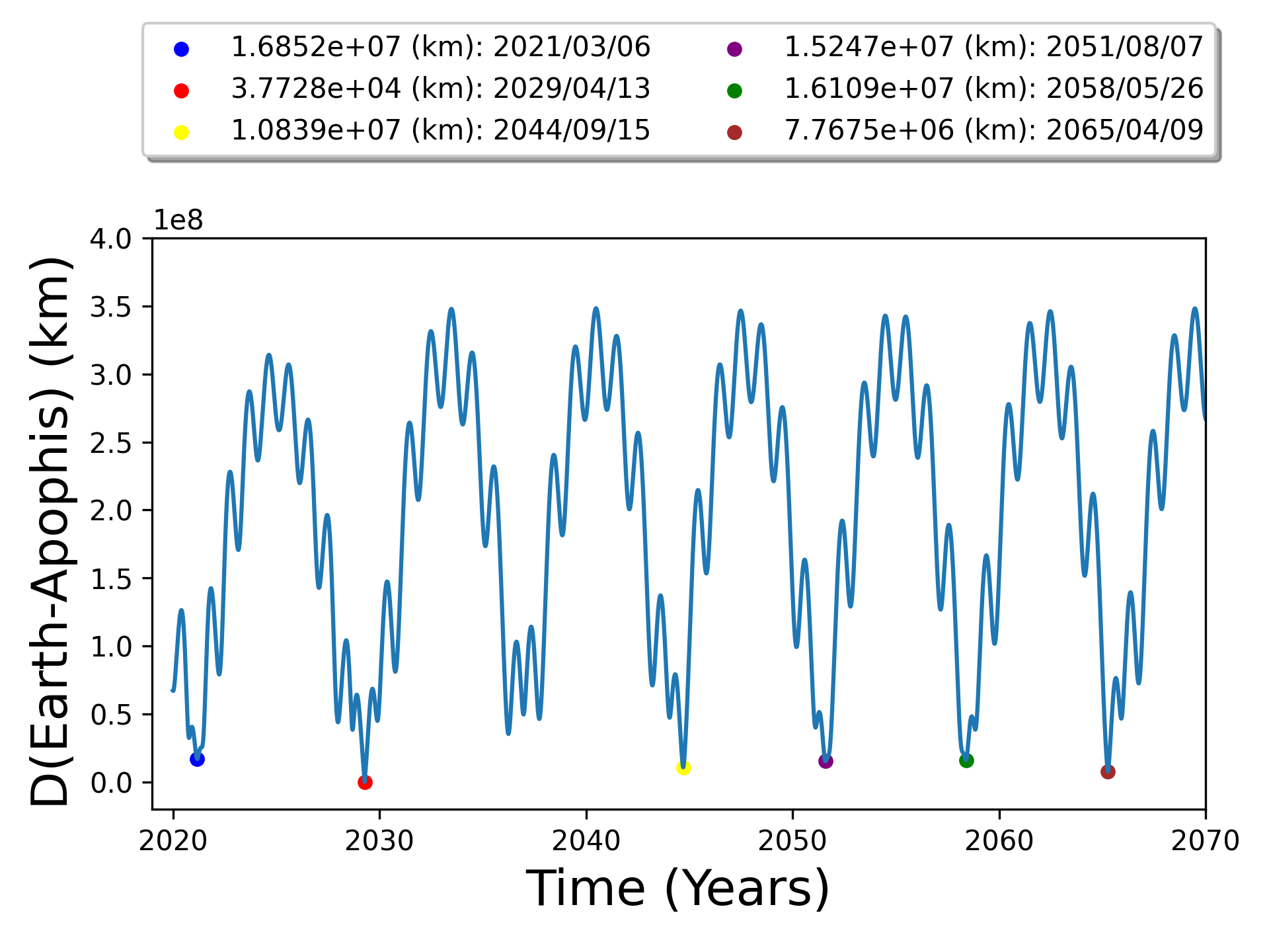
In this section, we study the dynamical system around (99942) Apophis during the close approach with our planet at $\sim$ 38,000 km on April 13${}^{\text{th}}$ 2029 (Fig. 9). For that purpose, we re-build the surfaces of section as presented in the previous section, with the difference that here we take into account the gravitational perturbations of the Sun, the 10 planet size bodies of our Solar System, including the Moon and Pluto, and the biggest 3 asteroids (Ceres, Pallas, and Vesta).

Figure 9: The close approach (Apophis-Eearth) provided by our numerical integration using Runge-Kutta methods with variable step size.

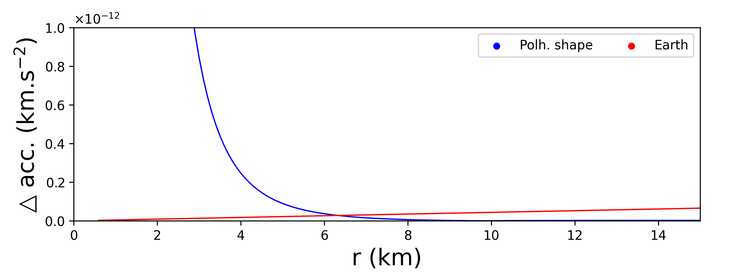
In fact, the Earth is by far the celestial body that most affects the dynamics around our target. In Fig. 10, we present the gravitational perturbation due to the polyhedral shape of Apophis (blue) and to the Earth (red) on the acceleration of a spacecraft close to the asteroid, 10 days before the minimum distance Apophis-Earth. We can see that the perturbation of our planet exceeds the perturbations of the shape beyond $\sim$6.4 km from the center of Apophis. This value is in accordance with the critical semimajor axis mentioned in Sanchez and Prado (2017) and Kinoshita and Nakai (1991), which is 5.719 km. However, this distance varies according to the position of our planet, as we can see in Fig. 11. At the instant of the close approach, for instance, the critical semimajor axis becomes $\sim$0.6 km. That justifies our focus on a region that stretches only 10 km from the center of our target.

Figure 10: The perturbation on the acceleration of a spacecraft close to (99942) Apophis, due to the perturbation of the polyhedral shape of the central body (Blue) and due to the Earth (Red), 10 days before the close approach.

The initial conditions (heliocentric positions and velocities) for all the bodies in Apophis system were provided by the JPL’s HORIZONS ephemerides on March 1, 2029, at a distance of 0.156 au from our planet, 43 days before the closest distance Apophis-Earth. We use the spherical harmonics up to degree and order four to expand the gravitational potential of the Earth and Moon, as presented in Sanchez et al. (2014); Sanchez and Prado (2017).

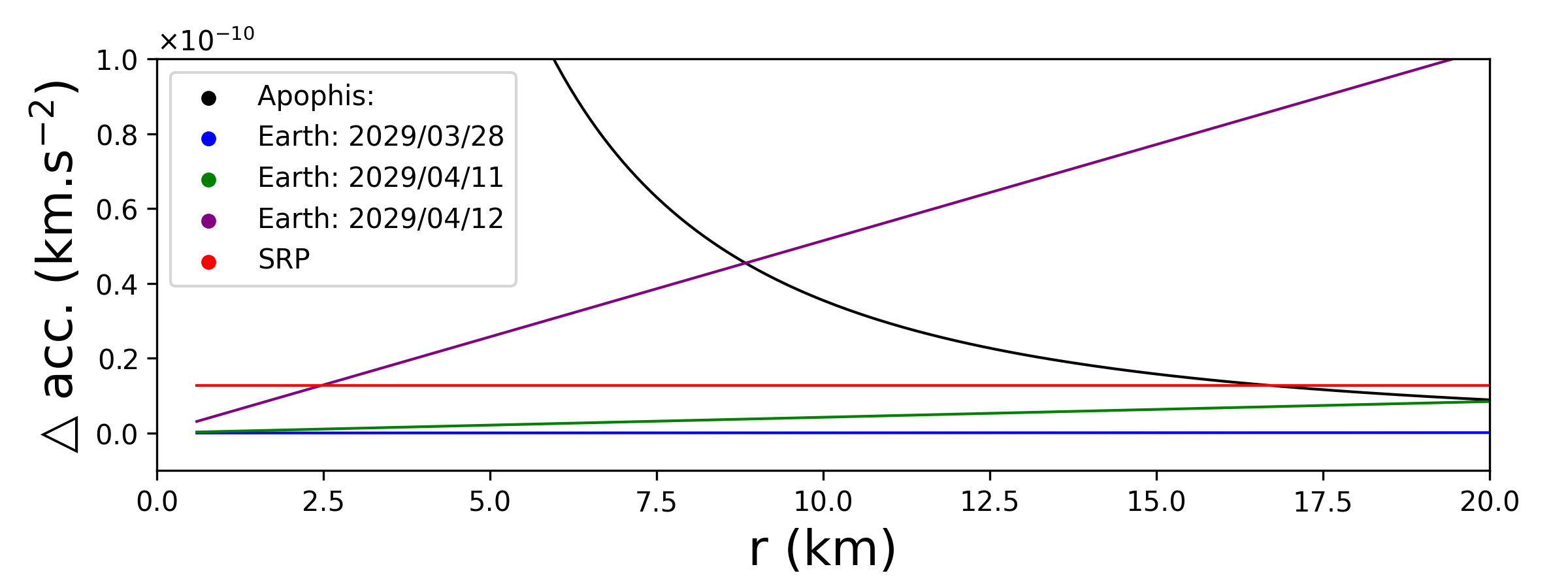
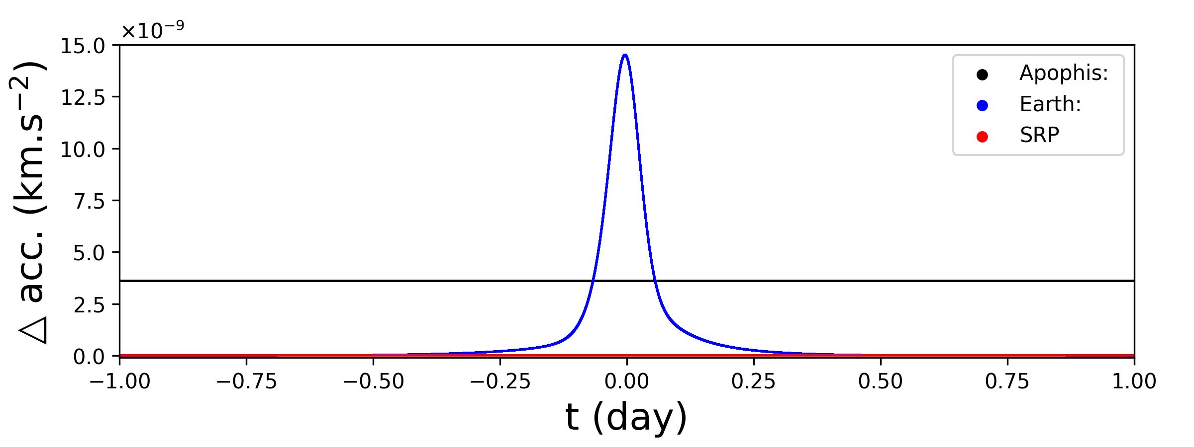
An important perturbation that arises from the Sun is the SRP. Besides the gravitational perturbations of the planets in our Solar System, above mentioned, we also considered the SRP in our study as described in Beutler (2005), where the radiation field due to the solar radiation is considered as parallel to the direction Sun-spacecraft. In this work, an OSIRIS-REx-like spacecraft is considered, presenting the following properties: a reflectance of 0.4, a mass of 1500 kg, and a cross-section of the spacecraft normal to the direction Sun-spacecraft of 25 m² with a mass-to-area ratio of 60 kg.m^-2, which yield a perturbation on the acceleration of the spacecraft that exceed the asteroid’s gravitational attraction at distances beyond $\sim$16.8 km close to the time of the close approach with Earth (1.00295 au from the Sun), as shown in Fig. 11 top panel, where we compare the perturbations on the acceleration of the spacecraft that is due to the SRP and due to our planet at different epochs in a region extending from 0.5 to 20 km from the surface of Apophis. In the bottom panel of this figure, we present the effect of these perturbations with respect to time, from one day before to one day after the CE on the acceleration of a spacecraft on a circular orbit at a distance of 1 km from the surface of our target. We can notice that the Earth perturbations quickly increases and becomes larger than the asteroid’s gravitational attraction itself. That leads to highly perturbed orbits in Apophis system, as we show later in this work.

Figure 11: Top panel: the perturbation on the acceleration of a spacecraft close to (99942) Apophis: due to SRP (Red), due to the Earth at different epoch (blue, green, and purple). Bottom panel: the evolution of these perturbations overtime on the acceleration of a spacecraft fixed at a distance of 1 km from the surface of Apophis.

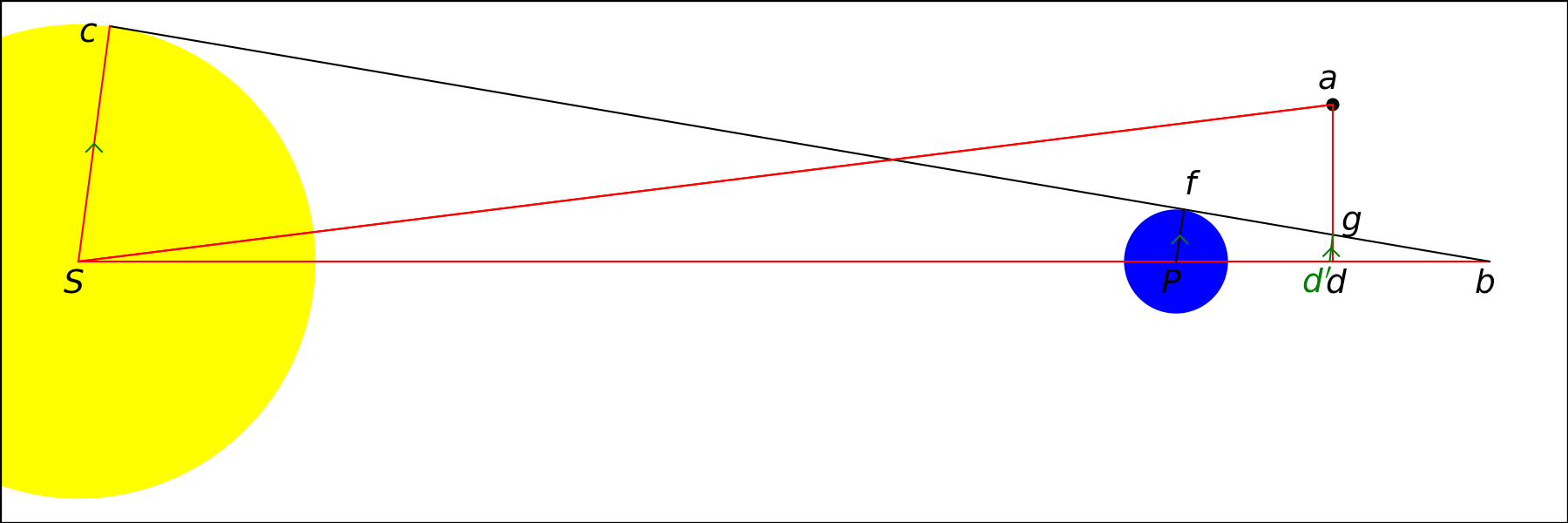
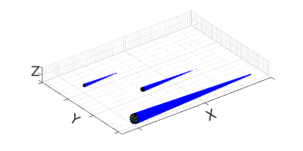
The shadowing of the sunlight by all the bodies in the system is also considered in our work. We assume that the Sun and the body in question are spherical with a radius of $R_{S}$ and $R_{P}$, respectively. The top panel of Fig. 12 illustrates the non-scaled shadow geometry for a body in the system. In fact, the sun is always far enough to consider the merger of $d$ and $d^{\prime}$ and $\cos(\widehat{aSd})\simeq 1$. With this consideration in mind, the spacecraft enters the shadow when $|\vec{ad}|\leq|\vec{gd}|$ and the vectors $\vec{PS}$ and $\vec{Pa}$ are in opposite directions, where the point $a$ is the position of the spacecraft where one want to define if shadow occurs or not. To demonstrate the effectiveness of this algorithm, we present, in the bottom panel of Fig. 12, the shadow of 3 spherical bodies in our simulation. However, it would be possible to consider the real shape of the body in the shadowing phenomenon by varying the value of $R_{P}$ at the point $f$, according to the polyhedral shape, using the CGAL library, which will affect significantly the execution time of our integration.

Figure 12: Non-scaled shadow geometry approach.

Overall, the equations of motion that describe the motion of a test particle around (99942) Apophis during the close approach with the Earth are given by:

$$\ddot{\text{r}}_{j} = -2\Omega\times\dot{\text{r}}_{j}-\Omega\times(\Omega\times\text{r}_{j})+U_{\text{r}_{j}}+\mathcal{A}(\mathcal{P})+$$

$$\text{P}_{\text{E}}+\text{P}_{\text{M}}+\nu\mathcal{A}(\text{P}_{\text{R}})$$

.
where: $i,j=1,2,...,15$ refer to the concerned body (spacecraft, Sun, 10 planets, and the biggest 3 asteroids). r is the position vector of the concerned body in the body-fixed frame, $\text{P}_{\text{E}}$ and $\text{P}_{\text{M}}$ are the accelerations due to the deformation of the Earth and of the moon, respectively. The vector $\mathcal{P}$ indicates the interaction between components $i$ and $j$ in the inertial frame.

$$\mathcal{P}=\sum_{i=1,i\neq j}^{15}\mathcal{G}m_{i}\big{(}\frac{\varUpsilon_{i}-\varUpsilon_{j}}{|\varUpsilon_{i}-\varUpsilon_{j}|^{3}}-\frac{\varUpsilon_{i}}{|\varUpsilon_{i}|^{3}}\big{)}$$

$\varUpsilon$ is the position vector in the inertial frame, $\mathcal{A}$ is an instantaneous rotation that takes the vector $\mathcal{P}$ from an inertial frame into a body-fixed frame. $\text{P}_{\text{R}}$ is the acceleration due to the direct radiation pressure applied only on the spacecraft, and $\nu$ is representing the shadowing phenomenon, taking the values 1 or 0, as defined earlier in this work.

$$\text{P}_{\text{R}}=(1+\eta)\leavevmode\nobreak\ \text{au}^{2}\leavevmode\nobreak\ \frac{A}{m}\frac{S}{c}\frac{\text{r}_{\text{s}}-\text{r}_{\odot}}{|\text{r}_{\text{s}}-\text{r}_{\odot}|^{3}}$$

.
where: $\eta$ is the reflectance properties of the spacecraft surface. au is the Astronomical Unit, $A$ is the cross section of the spacecraft normal to its direction to the Sun. $m$ is the mass of the spacecraft. $S$ is the solar constant and $c$ is the speed of light in vacuum. The value of $\frac{S}{c}$ is $4.56316\times 10^{-6}$ N/m² (Beutler, 2005). $\text{r}_{\text{s}}$ and $\text{r}_{\odot}$ are the coordinate vector of the spacecraft and the Sun, respectively. As we already mentioned, we considered the case of a spacecraft with low area-to-mass ratio ($\sim$ 0.017).

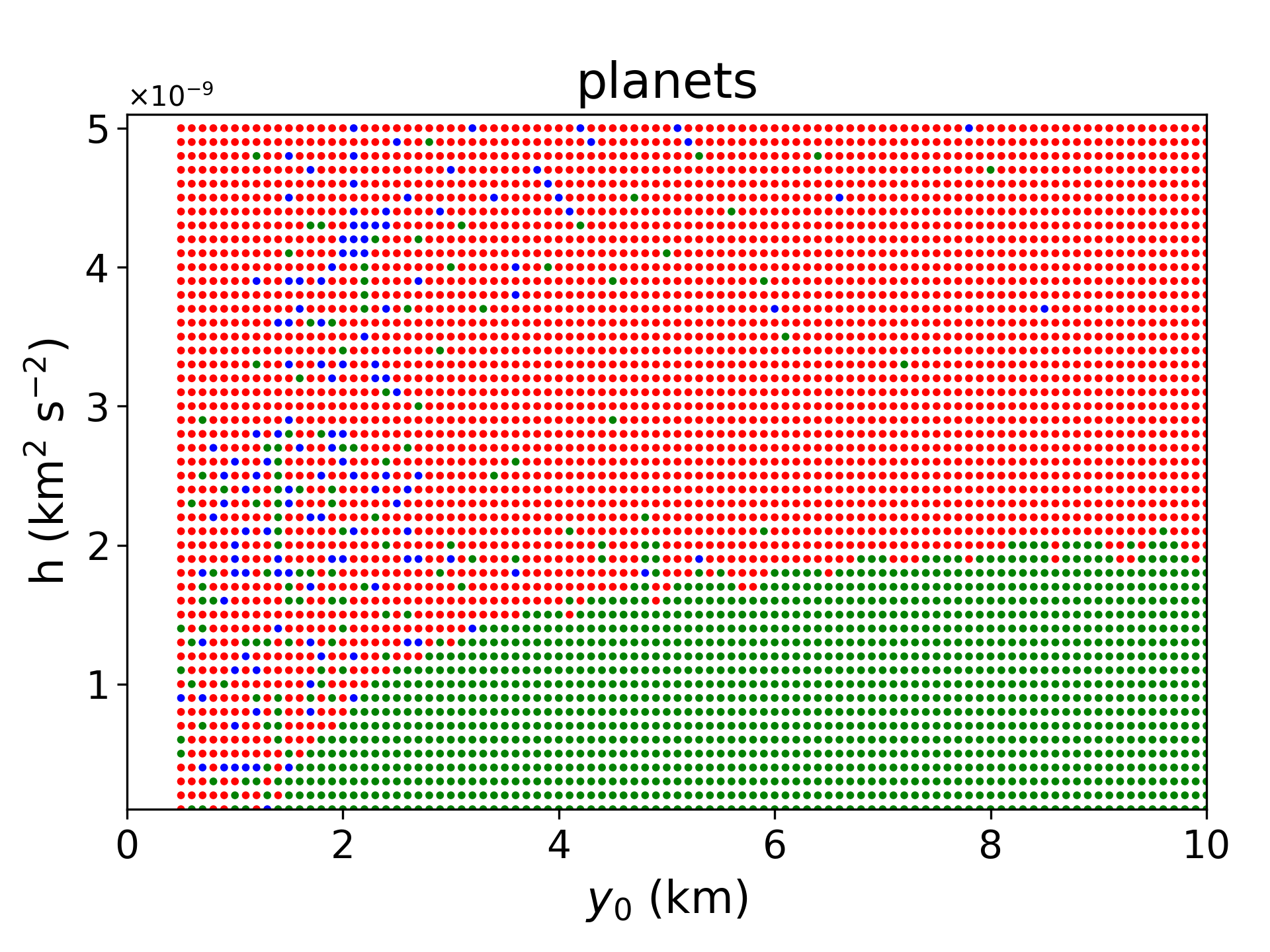
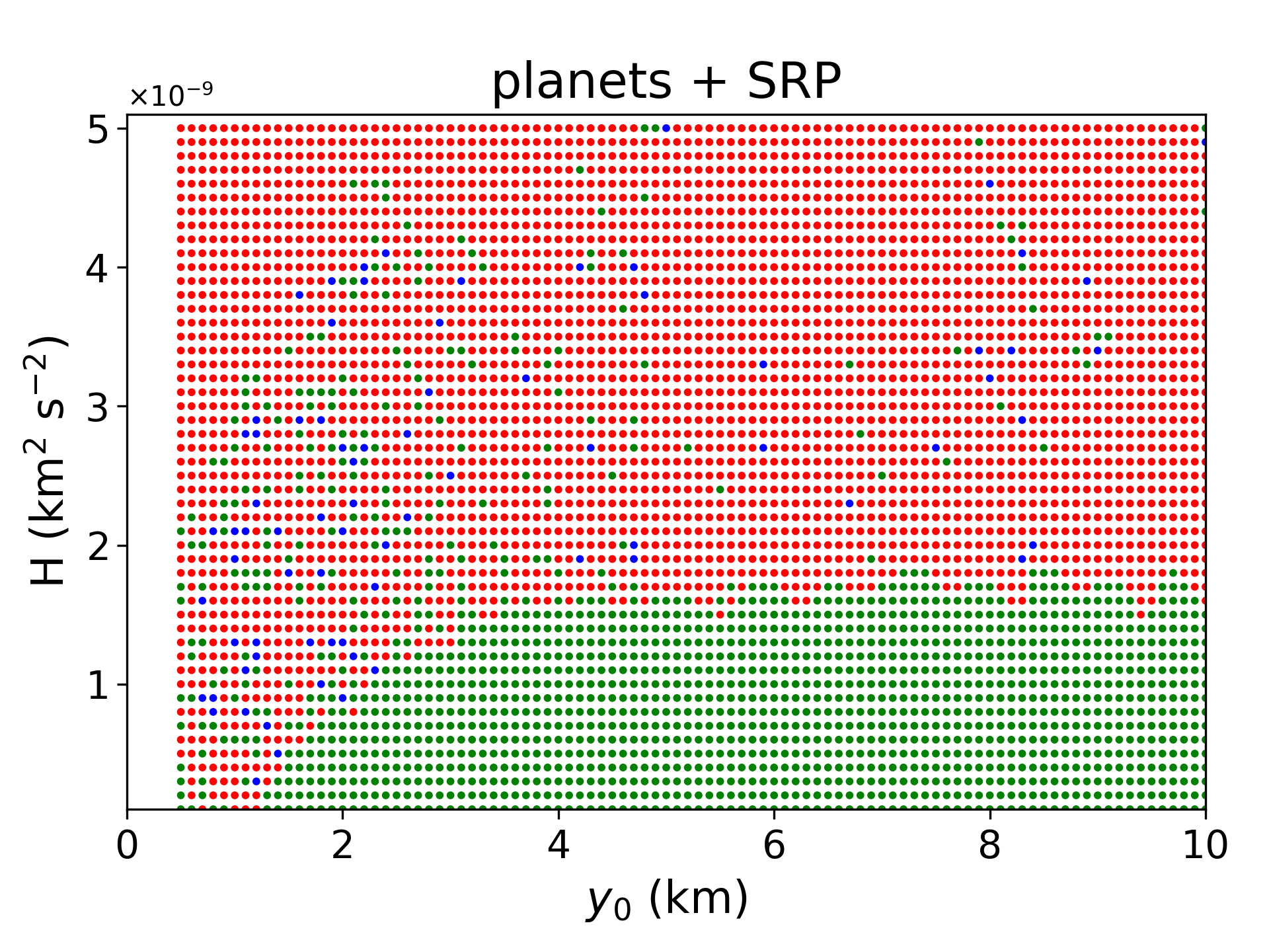
In Fig. 13, we present the type of all the orbits generated with our complete model, considering the planets in our Solar System without the SRP (top panel) and with the SRP (bottom panel). Comparing with Fig. 6 we can see that the planets in our Solar System destroyed the most of the orbits around Apophis, making the spacecraft collide or escape from the system, as we will see in more details later on in this section. We only found some bounded orbits very close to the central body. However, the SRP destabilized about 50% of them, changing their distribution in the ($dy_{0}$, h) plane. Such a drastic effect of the SRP was already seen in Chanut et al. (2017) studying the dynamics around the asteroid Bennu, and also in Sanchez and Prado (2019) studying the Less-Disturbed Orbital Regions Around the Near-Earth Asteroid 2001 SN₂₆₃.

Figure 13: Type of orbits around the asteroid (99942) Apophis. Considering or not the perturbations of the planets in our Solar System and the SRP. The colour symbols are the same as in Fig. 6.

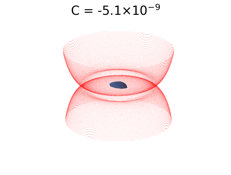
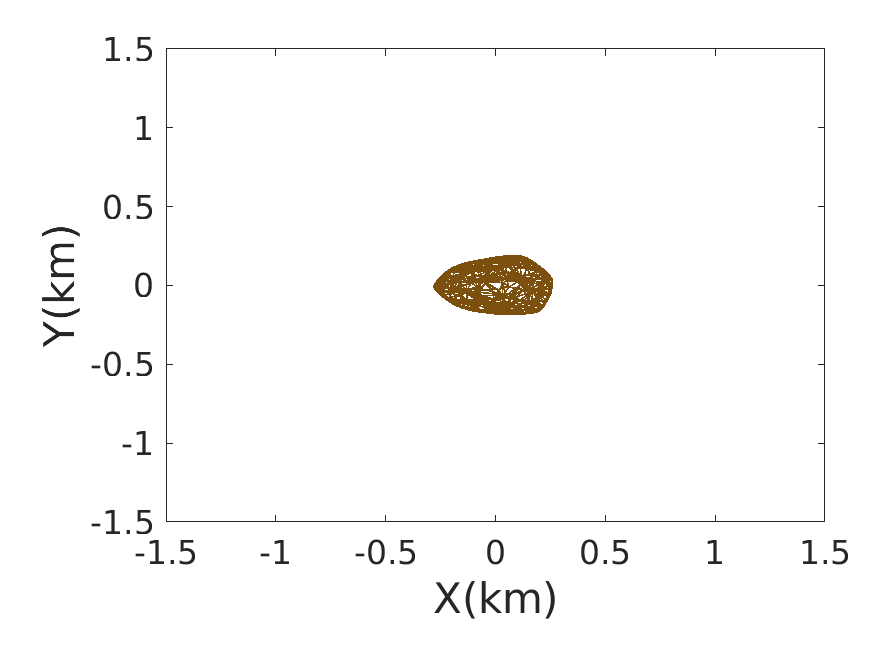
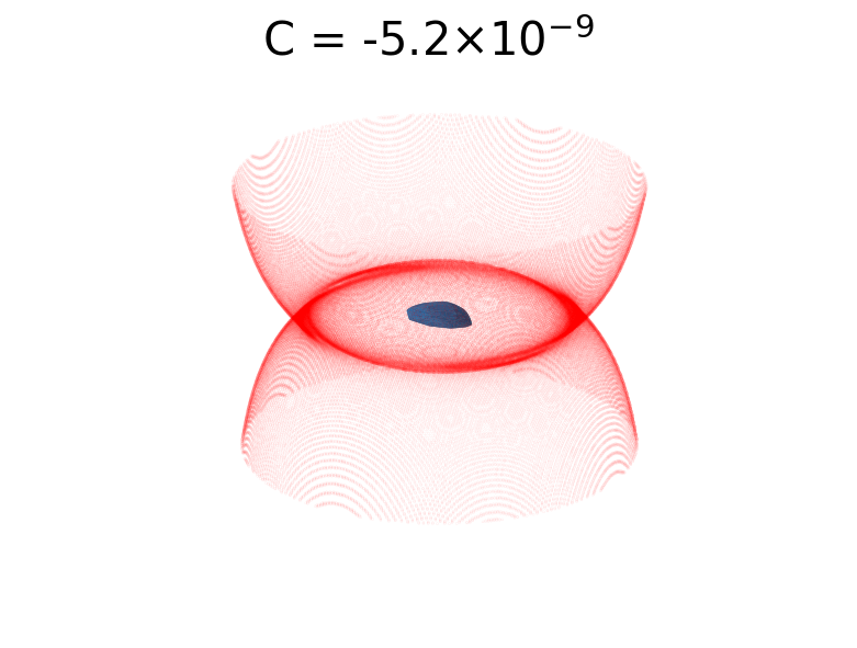
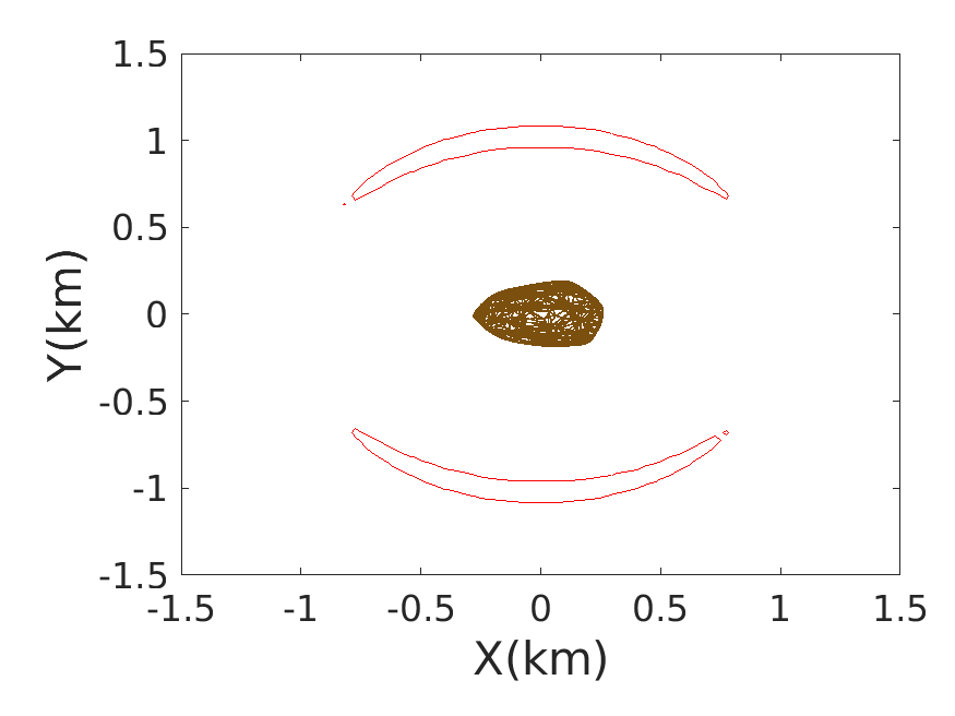
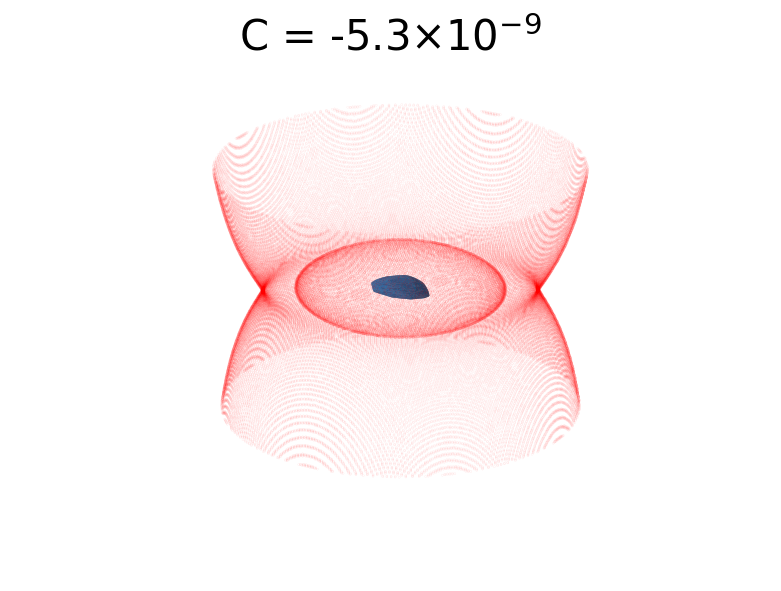
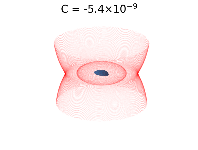
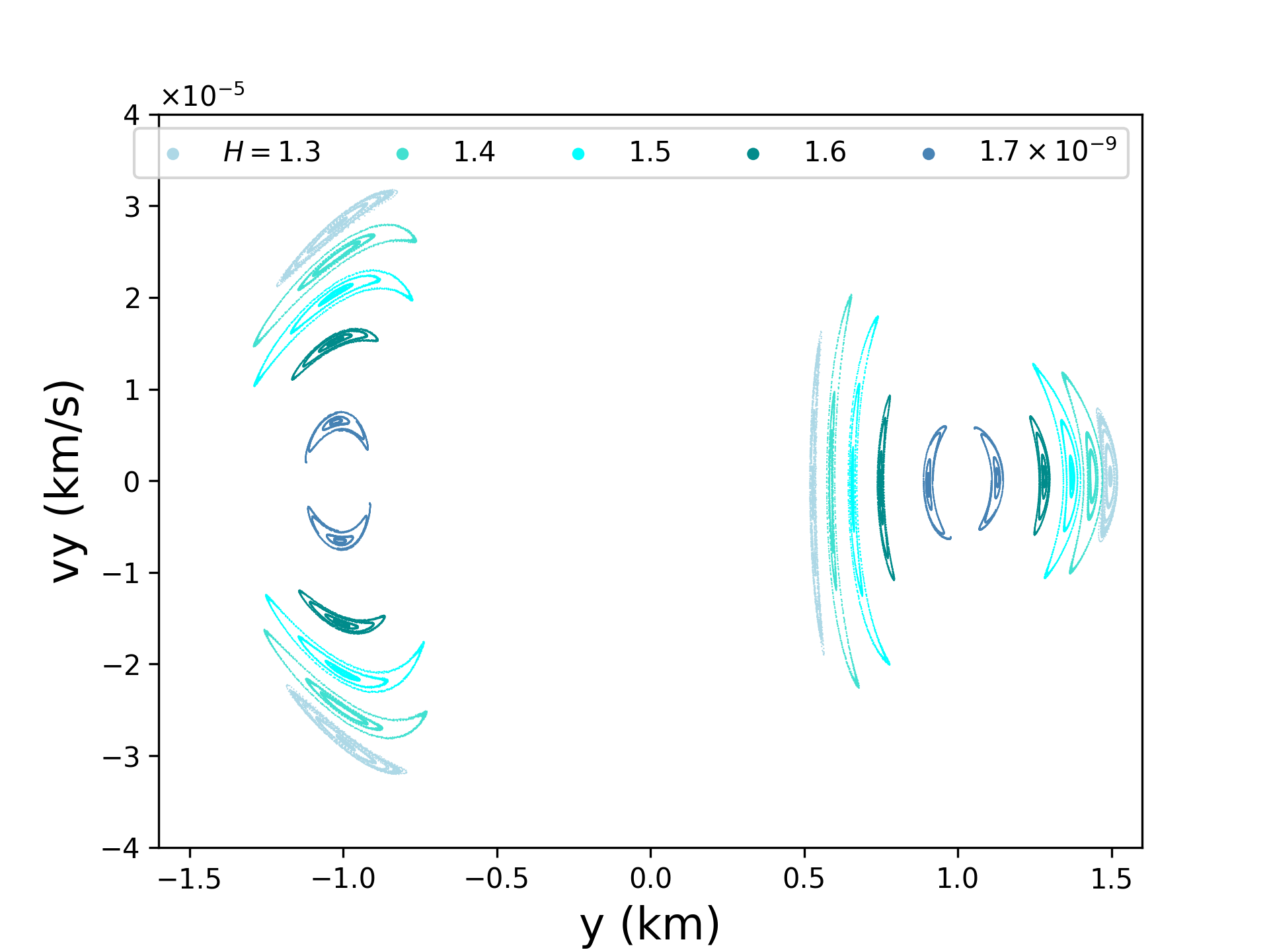
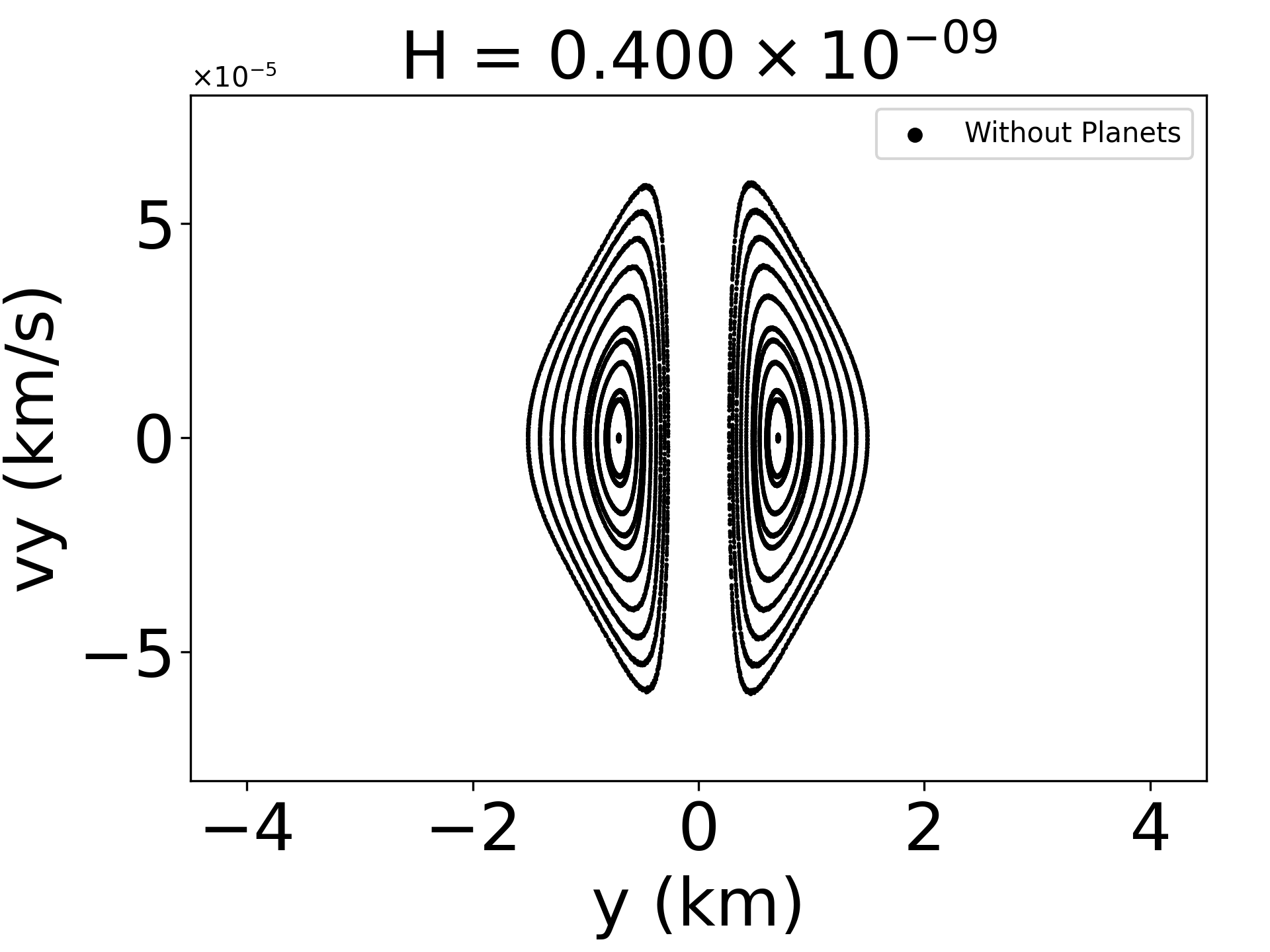
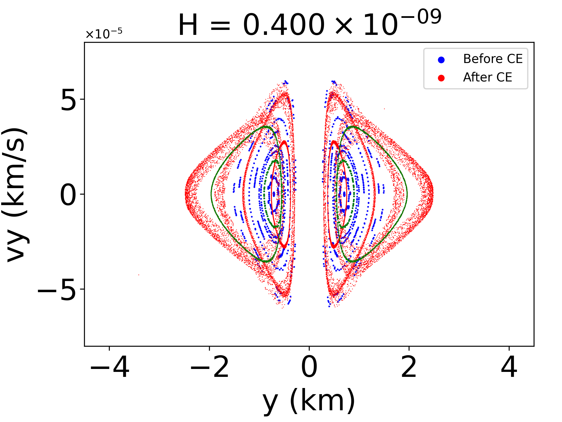
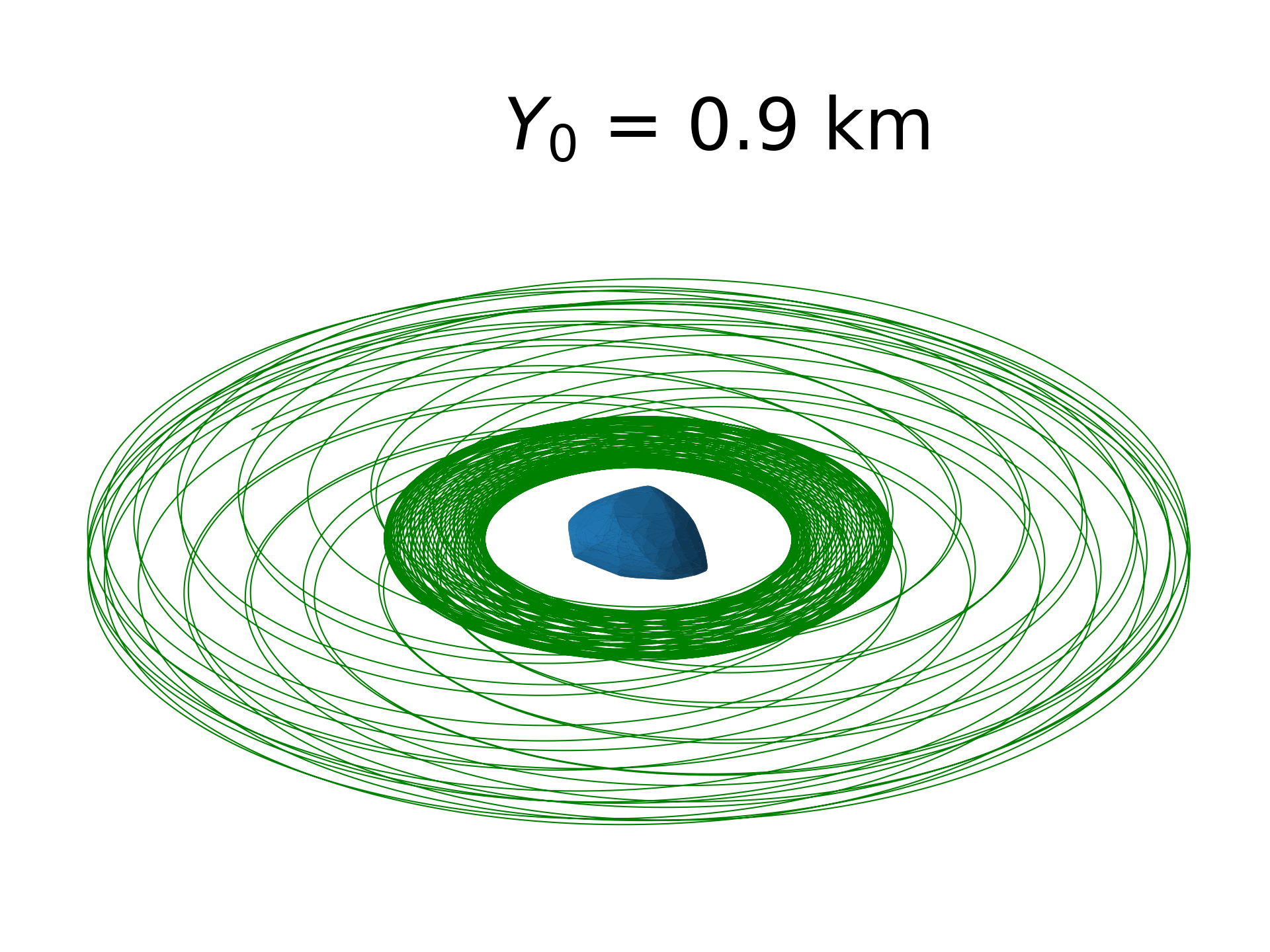
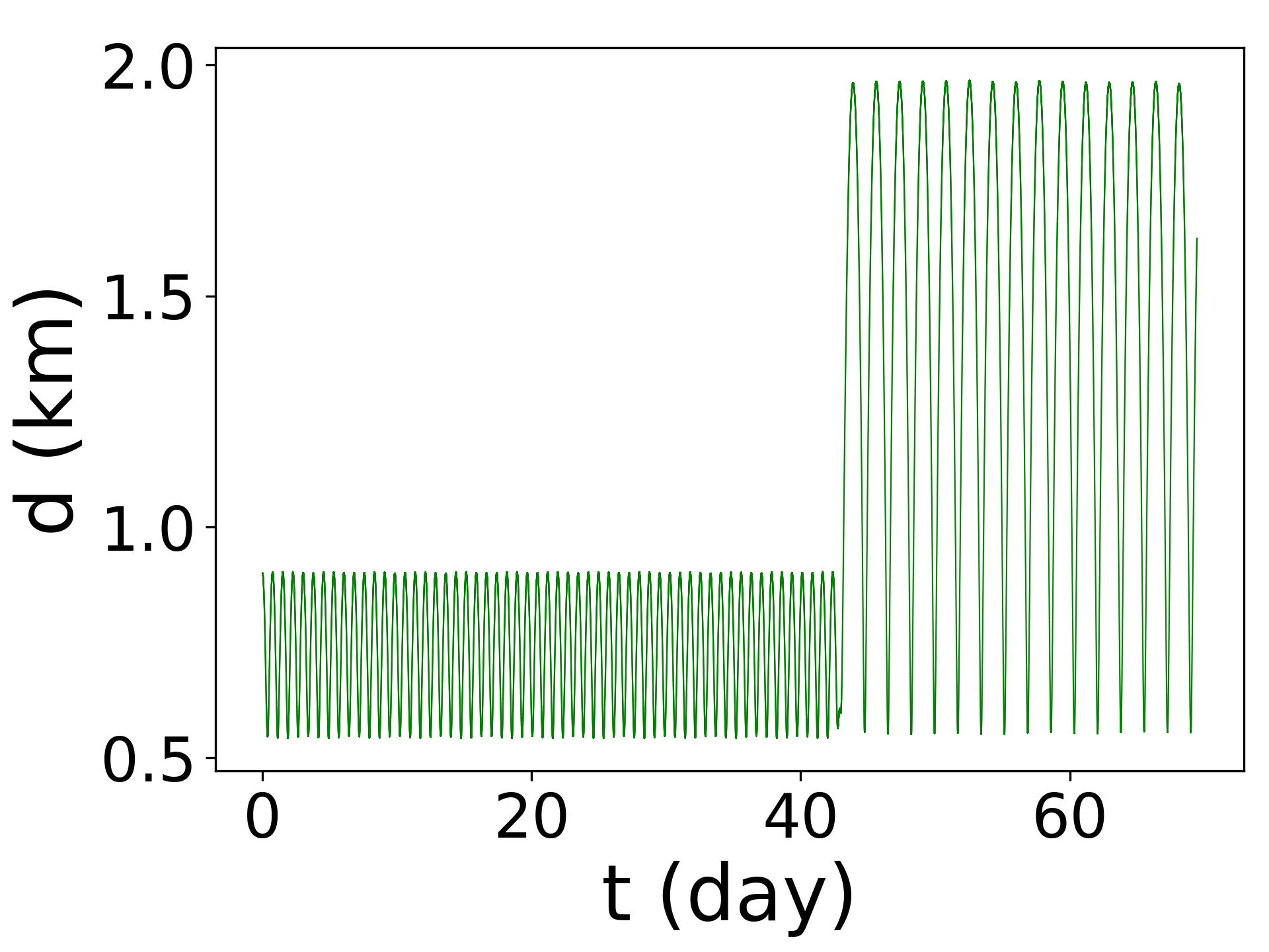
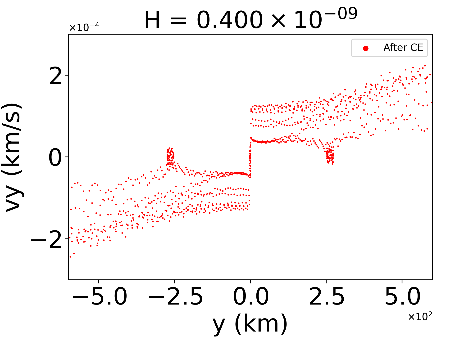
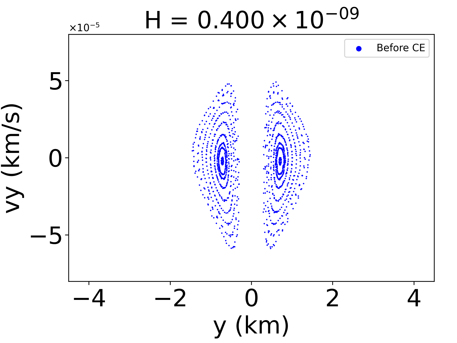
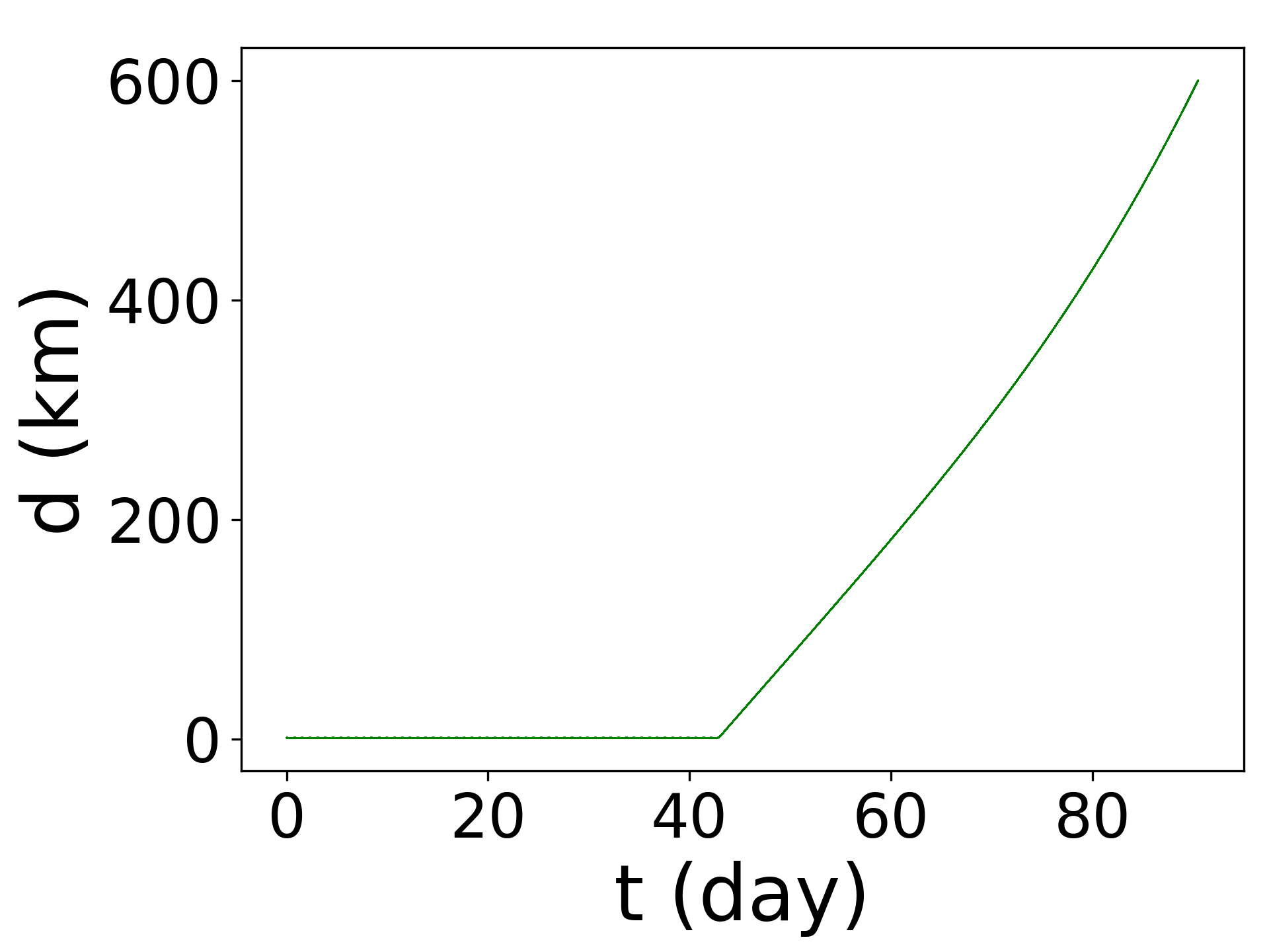
In order to better understand the dynamics around our target, we present, in Fig. 14, the surfaces of the section for $H=0.4\times 10^{-9}$, starting from March 1, 2029 considering (top right panel) or not (top left panel) the perturbations of the planets in the Solar System and neglecting the SRP. Comparing these two panels, we can notice that a new configuration appears after 43 days of our integration, that correspond to the instant of the close approach with our planet. This point will be seen clearly by following the evolution of the distance between our test particle and the central body, as in the bottom panels in Fig. 14, where we show an example of bounded orbits around Apophis. For the seek of clarity, we presented the first 70 days of the orbit. However, including the SRP in our model changes completely the structure of the surfaces of the section, giving the tendency for highly chaotic orbits. In Fig. 15 we present our results for $h=0.4\times 10^{-9}$. Again, we notice that the distance between our test particle and the central body significantly changed just after the close approach with our planet. We should now turn our attention to identify the less perturbed region around Apophis.

Figure 14: Intersection points of orbits around (99942) Apophis, starting from March 1, 2029. Here, we considered the perturbation from the remaining bodies in the Solar System and neglected the SRP.

Figure 15: Intersection points of orbits around (99942) Apophis, starting from March 1, 2029. Here, we considered the perturbation from the remaining bodies in the Solar System and the SRP.

5 Search for less perturbed regions around (99942) Apophis

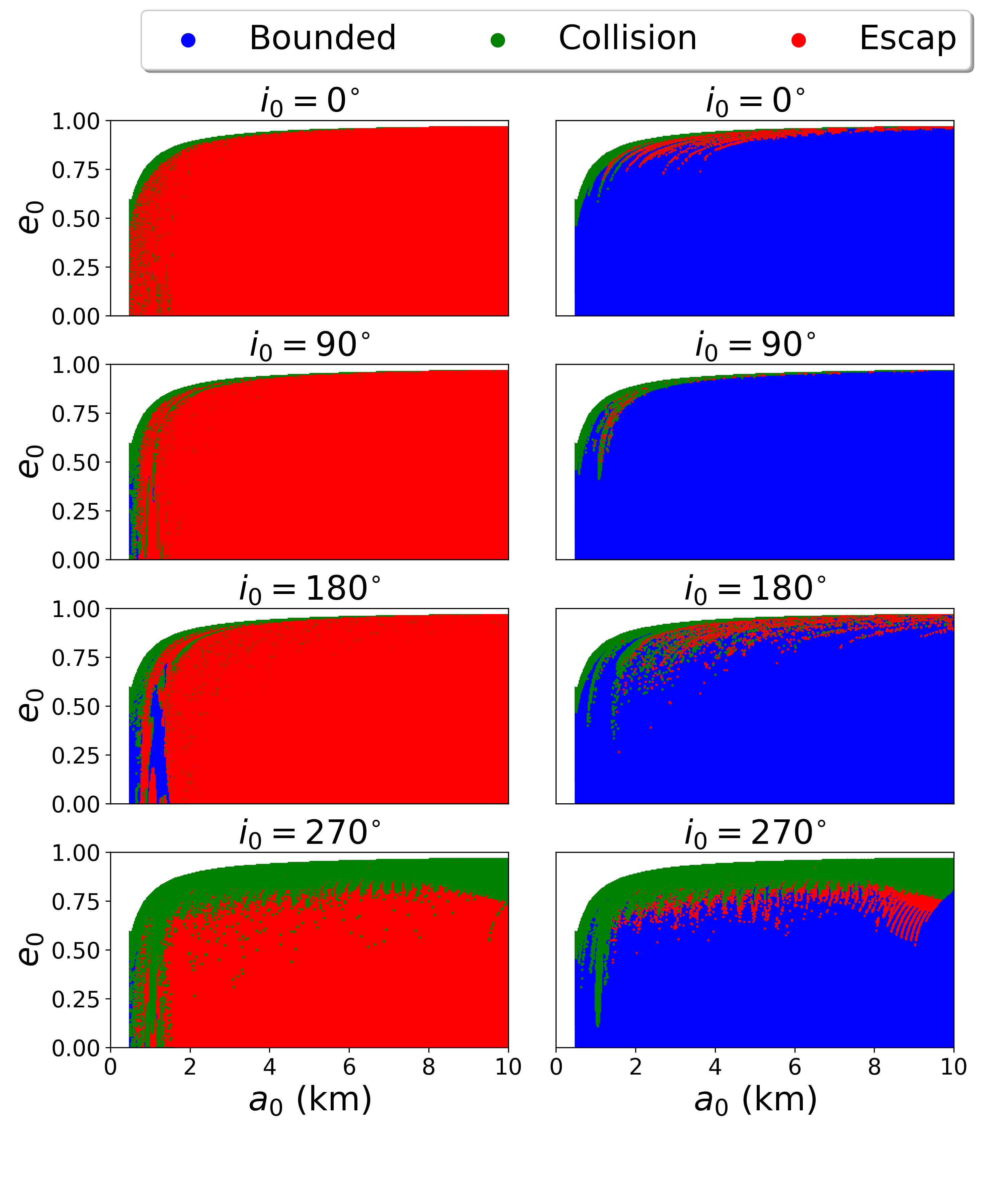
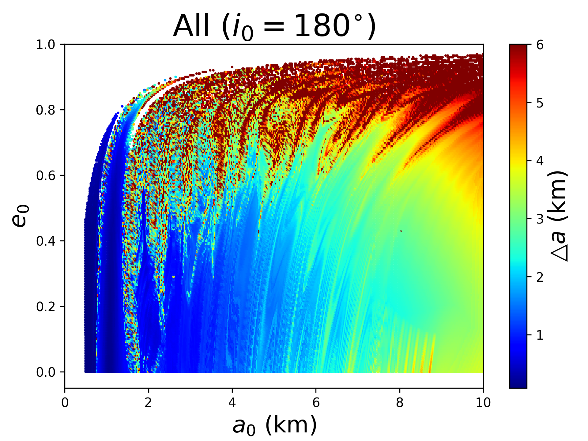
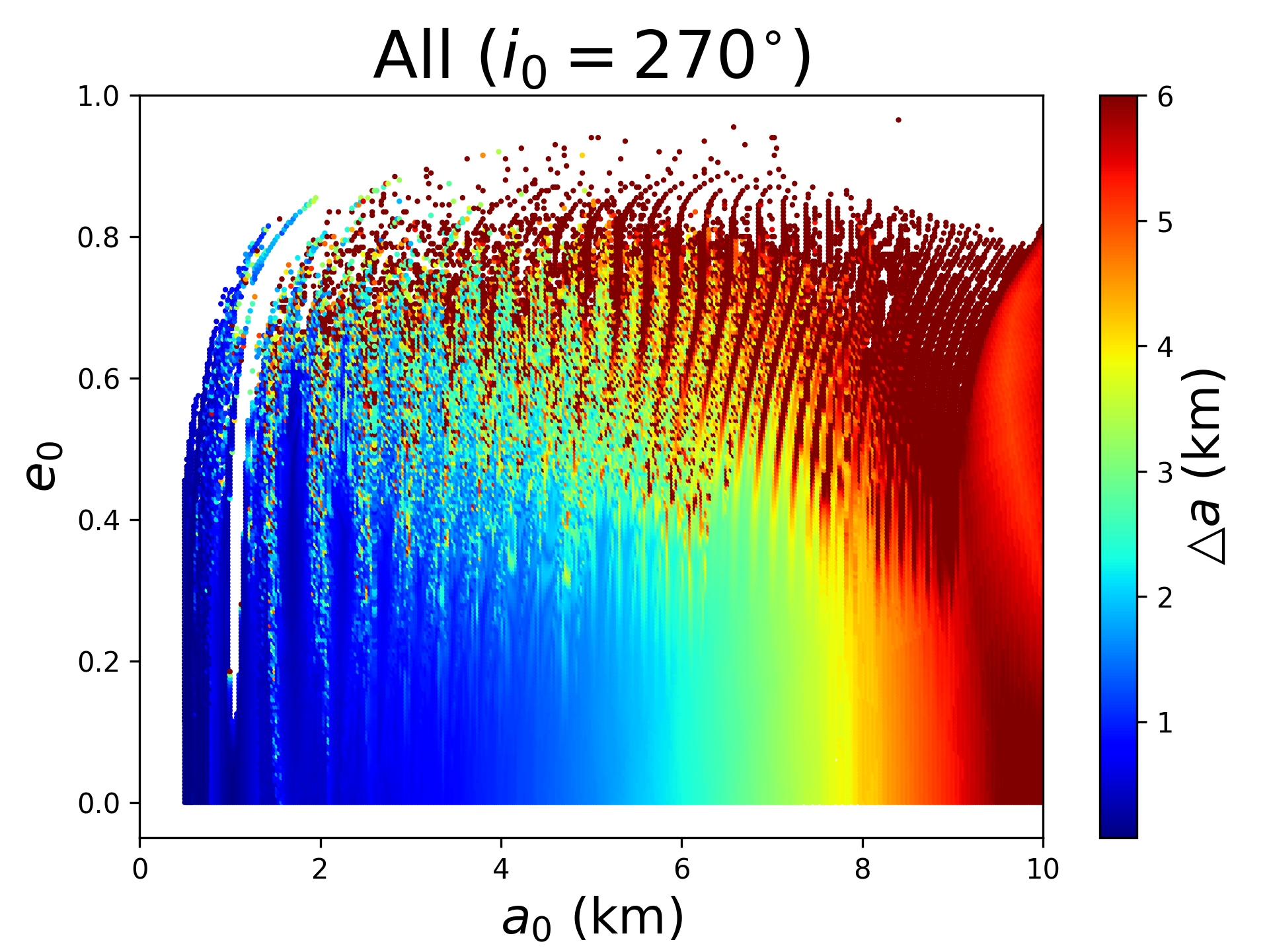
In order to identify suitable regions to place a spacecraft around (99942) Apophis on March 1, 2029, we made a numerical analysis of orbits in a region with a semimajor axis between 0.5 and 10 km from the center of (99942) Apophis with an interval of 25 m. We vary the initial eccentricities from 0 to 1 with a step size of 0.005, and tested 4 different inclinations ($0^{\circ}$, $90^{\circ}$, $180^{\circ}$, $270^{\circ}$). The argument of the perigee ($\omega$), the longitude of ascending node ($\Omega$), and the mean anomaly of the small probes are initially $0^{\circ}$. Again, the vast majority of the tested orbits collide or escape from the system at the time of the close approach with Earth. In Fig. 16 we present the type of all the tested orbits integrated for 40 days (right column) and 60 days (left column). Considering that left and right panels correspond to the same initial conditions evolved by the same equations but for a different final time, it means that most of the orbits escape after 40 days of integration due to the close approach with the Earth.

Figure 16: Type of orbits around the asteroid (99942) Apophis for 60 days (left column) and 40 days (right column) starting from March 1, 2029.

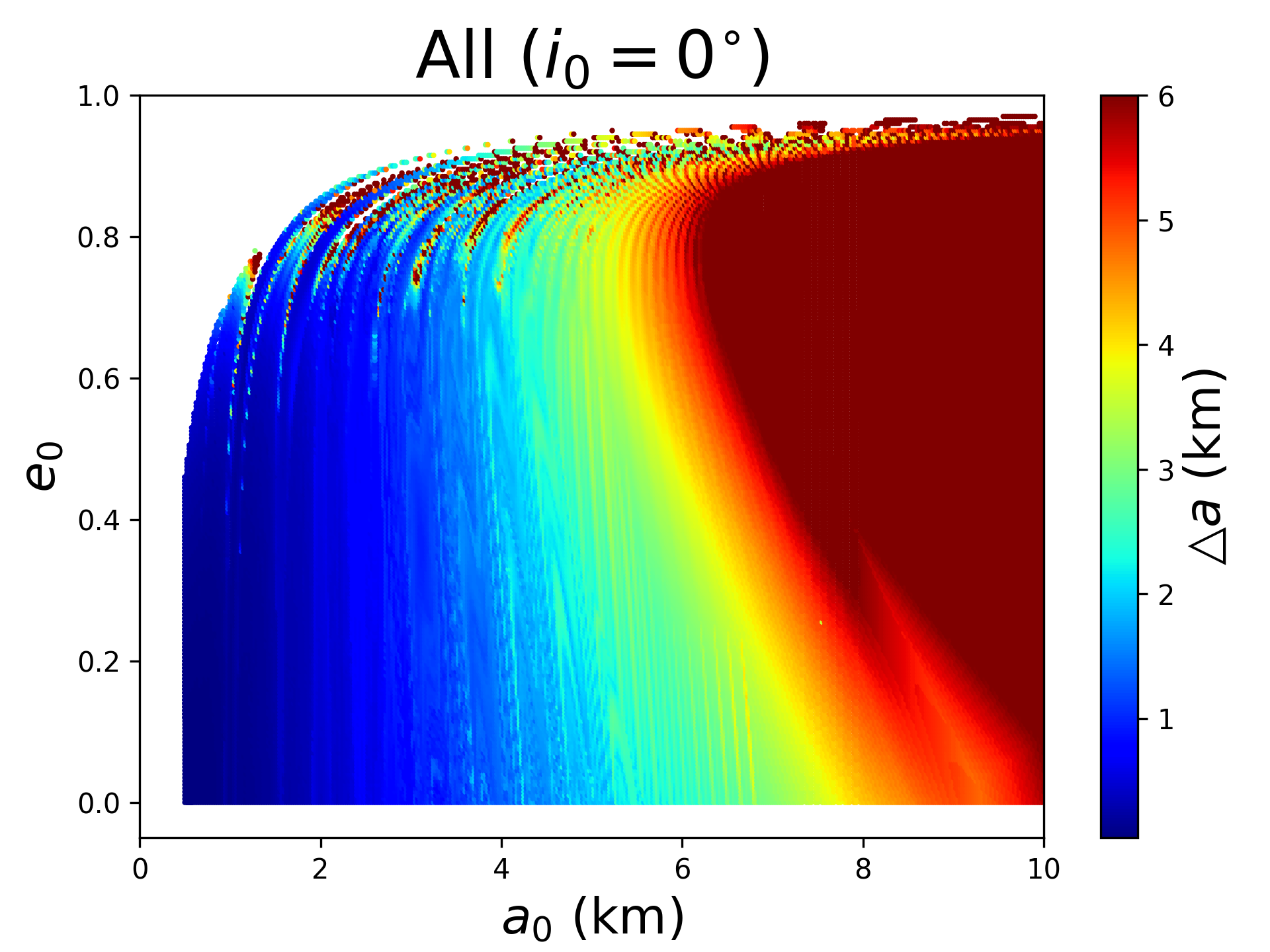
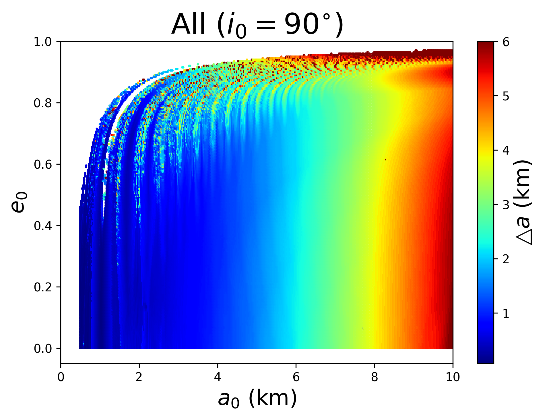
Considering our results for 40 days of integration, we use the variation of the semimajor axis ($\bigtriangleup a$) as a criterion to identify the less perturbed regions in the system. Our results are presentd in Fig. 17. The smooth parts of the map with small values of $\bigtriangleup a$ could be a possible option to insert a spacecraft into natural orbits around Apophis before the close approach with our planet. The minimum value founded of this variation is 0.05 km and a variation of the corresponding eccentricity is ($\bigtriangleup e$) of 0.128, which is still a non-negligible variation presented in Fig. 18. However, an interesting part of the region around Apophis is heavily perturbed, that appears in the map beyond 4 km from the center of Apophis.

Figure 17: The variation maps of the semimajor axis coming from the ensemble perturbations on real system of Apophis.

Figure 18: An example of the less perturbed orbits close of Apophis over 40 days.

6 Orbital control around (99942) Apophis

As we already saw in this paper, the most problematic behaviors of the dynamics around our target come from the close approach with our planet. In order to solve the stabilization problem for the system of equation 4, we applied in this section the robust path following control law as presented in Negri and Prado (2020a, b), The advantage of a path following control to a reference tracking control is that in the first situation, only the geometry of the orbit is controlled, with no a priori time parameterization. A detailed discussion of the applicability and practical considerations of the path following the law derived in Negri and Prado (2020a) for asteroid missions is done in Negri and Prado (2020b). The acceleration correction is calculated in the radial-transverse-normal coordinates (RTN), where the versors of the spacecraft are defined as follows:

$$\hat{r}=\frac{\vec{r}}{r},\leavevmode\nobreak\ \leavevmode\nobreak\ \leavevmode\nobreak\ \leavevmode\nobreak\ \leavevmode\nobreak\ \leavevmode\nobreak\ \leavevmode\nobreak\ \leavevmode\nobreak\ \leavevmode\nobreak\ \leavevmode\nobreak\ \leavevmode\nobreak\ \leavevmode\nobreak\ \hat{h}=\frac{\vec{h}}{h},\leavevmode\nobreak\ \leavevmode\nobreak\ \leavevmode\nobreak\ \leavevmode\nobreak\ \leavevmode\nobreak\ \leavevmode\nobreak\ \leavevmode\nobreak\ \leavevmode\nobreak\ \leavevmode\nobreak\ \leavevmode\nobreak\ \leavevmode\nobreak\ \leavevmode\nobreak\ \hat{\theta}=\hat{h}\times\hat{r}$$

where, $\vec{h}=\vec{r}\times\dot{\vec{r}}$ is the angular momentum of the spacecraft, $\vec{r}$ and $\dot{\vec{r}}$ are the position and velocity vectors, in the frame where the orbit will be controlled. We defined the eccentricity vector ($\vec{e}$) and the sliding surface ($\vec{s}$) as

$$\vec{e} = \frac{1}{\mu}\bigg{(}\dot{\vec{r}}\times\vec{h}-\mu\hat{r}\bigg{)}$$

$$\vec{s} = \begin{bmatrix}(\vec{e}-\vec{e}_{d}).(\lambda_{R}\hat{r}+\hat{\theta})\\ h-h_{d}\\ \hat{h}_{d}.(\lambda_{N}\hat{r}+\hat{\theta})\end{bmatrix}$$

where, $\lambda_{R}$ and $\lambda_{N}$ are design parameters. They will determine the asymptotic convergence to the sliding surface. In our application, they are fixed to a value of 0.002. $\vec{e}_{d}$ and $\hat{h}_{d}$ are the desired eccentricity vector and angular momentum versor, respectively. They are given by:

$$\vec{e}_{d} = \begin{bmatrix}\cos(\Omega_{d})\cos(\omega_{d})-\sin(\Omega_{d})\sin(\omega_{d})\cos(i_{d})\\ \sin(\Omega_{d})\cos(\omega_{d})-\cos(\Omega_{d})\sin(\omega_{d})\cos(i_{d})\\ \sin(\omega_{d})\sin(i_{d})\end{bmatrix}$$

$$\hat{h}_{d} = \begin{bmatrix}\sin(i_{d})\sin(\Omega_{d})\\ -\sin(i_{d})\cos(\Omega_{d})\\ \cos(i_{d})\end{bmatrix}$$

where, $i_{d},\Omega_{d},$ and $\omega_{d}$ are the desired inclination, longitude of the ascending node and argument of periapsis, respectively. The acceleration corrections in the RTN coordinates can be written as:

$$\vec{u}_{RTN}=(U_{R},U_{T},U_{N})=-F^{-1}\big{(}G+K\text{sat}(\vec{s},\vec{\Phi})\big{)}$$

where,

$$F = \frac{1}{h\mu}\begin{bmatrix}-h^{2}&(2\lambda_{R}h-(\dot{\vec{r}}.\hat{r})r)h&-\mu r\vec{e}_{d}.\hat{h}\\ 0&\mu rh&0\\ 0&0&\mu r\hat{h}_{d}.\hat{h}\end{bmatrix}$$

$$G = \frac{h}{r^{2}}\begin{bmatrix}(\vec{e}-\vec{e}_{d}).(\lambda_{R}\hat{\theta}-\hat{r})\\ 0\\ \hat{h}_{d}.(\lambda_{N}\hat{\theta}-\hat{r})\end{bmatrix}$$

$$K = \begin{bmatrix}0.001&0.0&0.0\\ 0.000&0.1&0.0\\ 0.000&0.0&0.1\end{bmatrix},\Phi=\begin{bmatrix}0.005\\ 0.500\\ 0.050\end{bmatrix}$$

$\text{sat}(\vec{s},\vec{\Phi})$ is the saturation function, proposed to avoid the discontinuous control input.

$$\text{sat}(\alpha,\beta)=\begin{cases}+1\qquad\alpha>\beta\\ +\frac{\alpha}{\beta}\quad-\beta\leq\alpha\leq\beta\\ -1\qquad\alpha<-\beta\end{cases}$$

Finally, the acceleration corrections in our frame of reference is given by

$$\vec{u}=U_{R}\hat{r}+U_{T}\hat{\theta}+U_{N}\hat{h}$$

For more detailed and deeper analysis on all the theoretical considerations considering all practical aspects, we refer the reader to Negri and Prado (2020a, b).

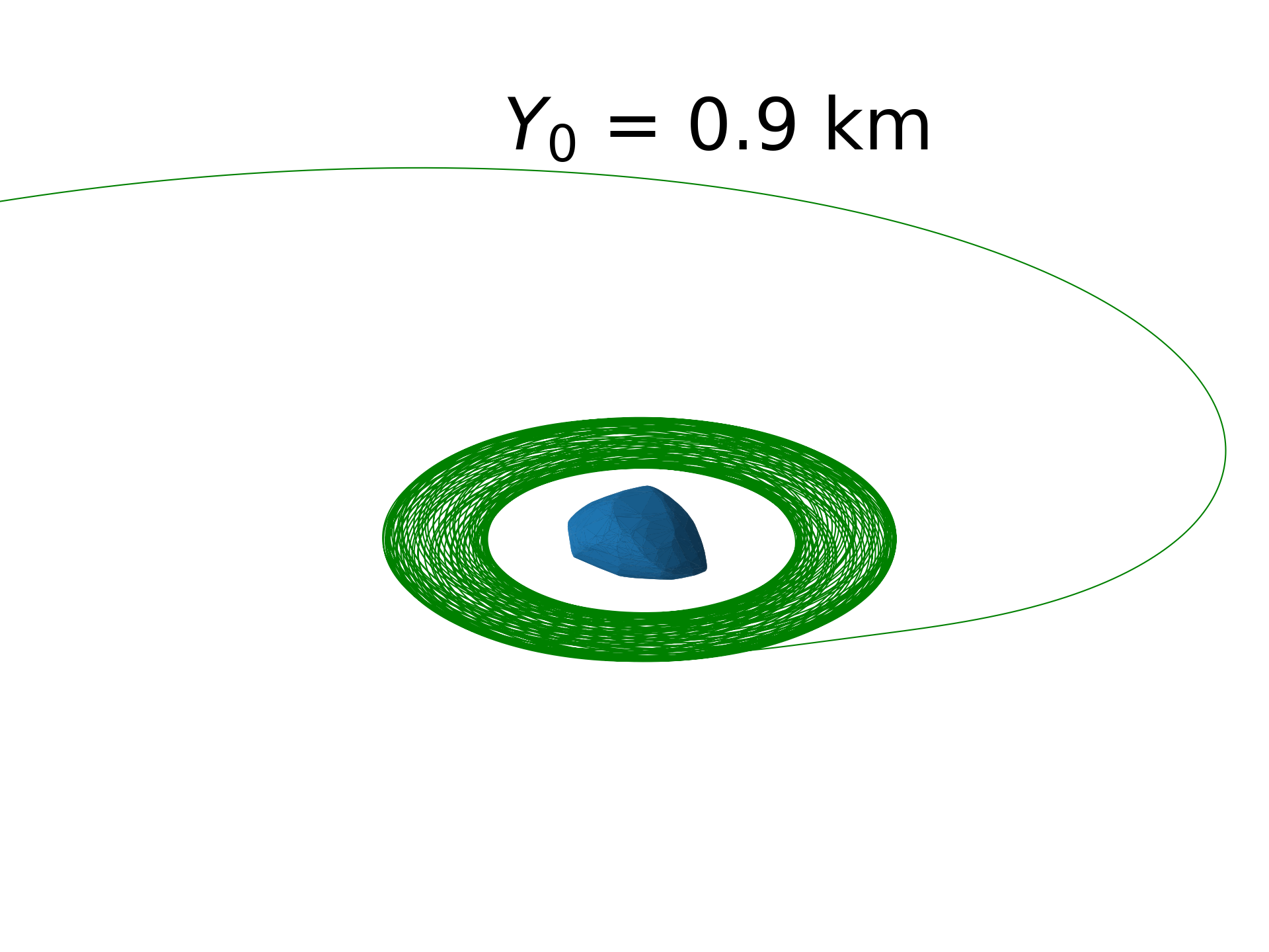
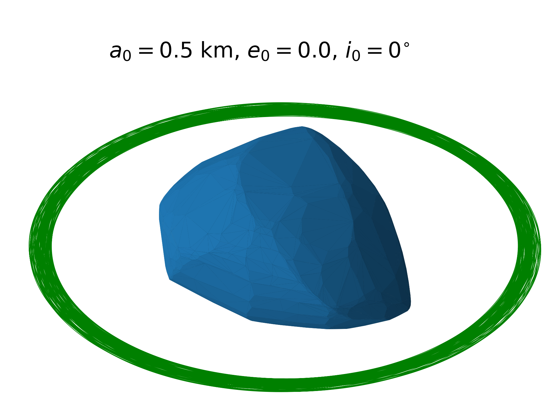
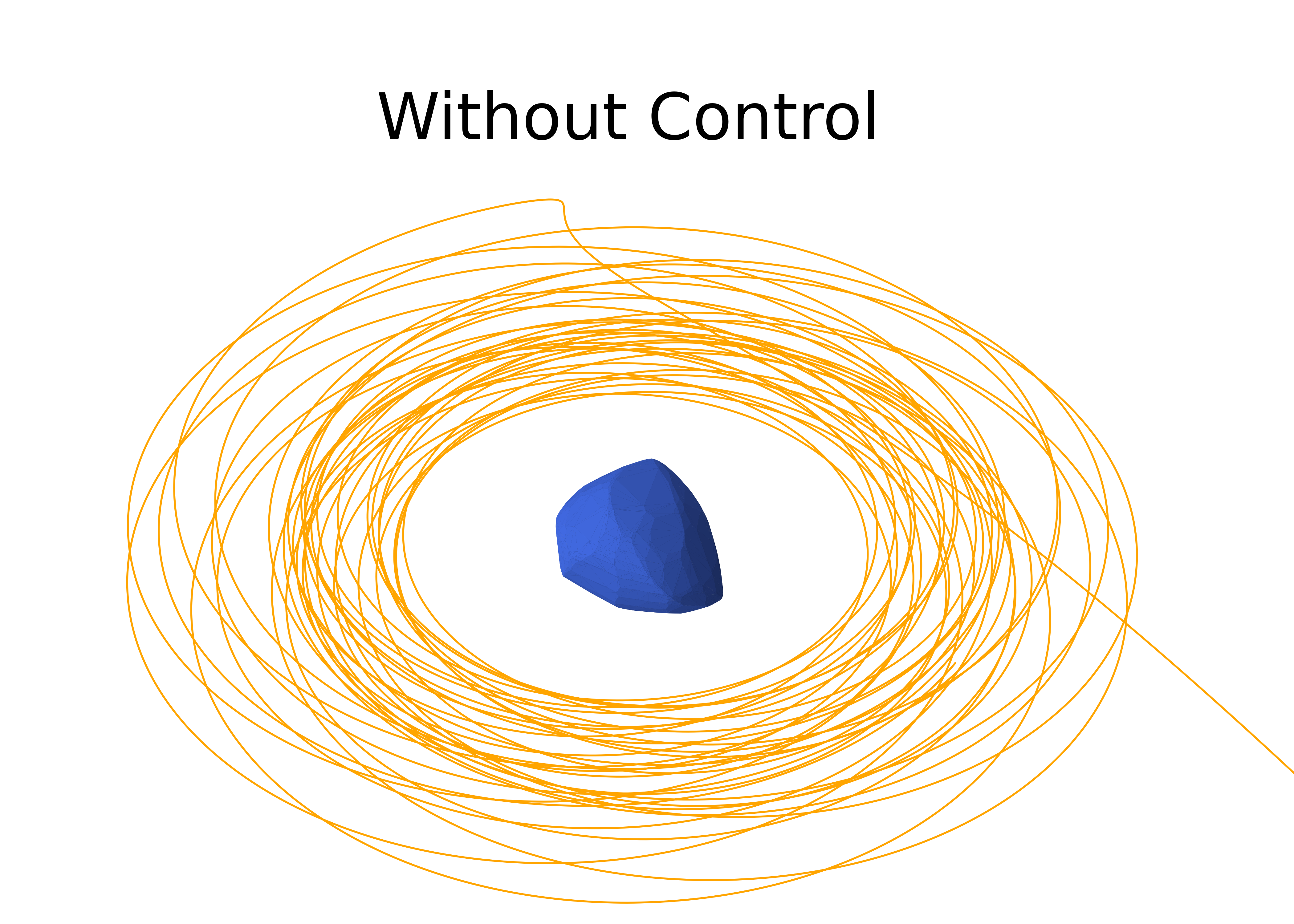
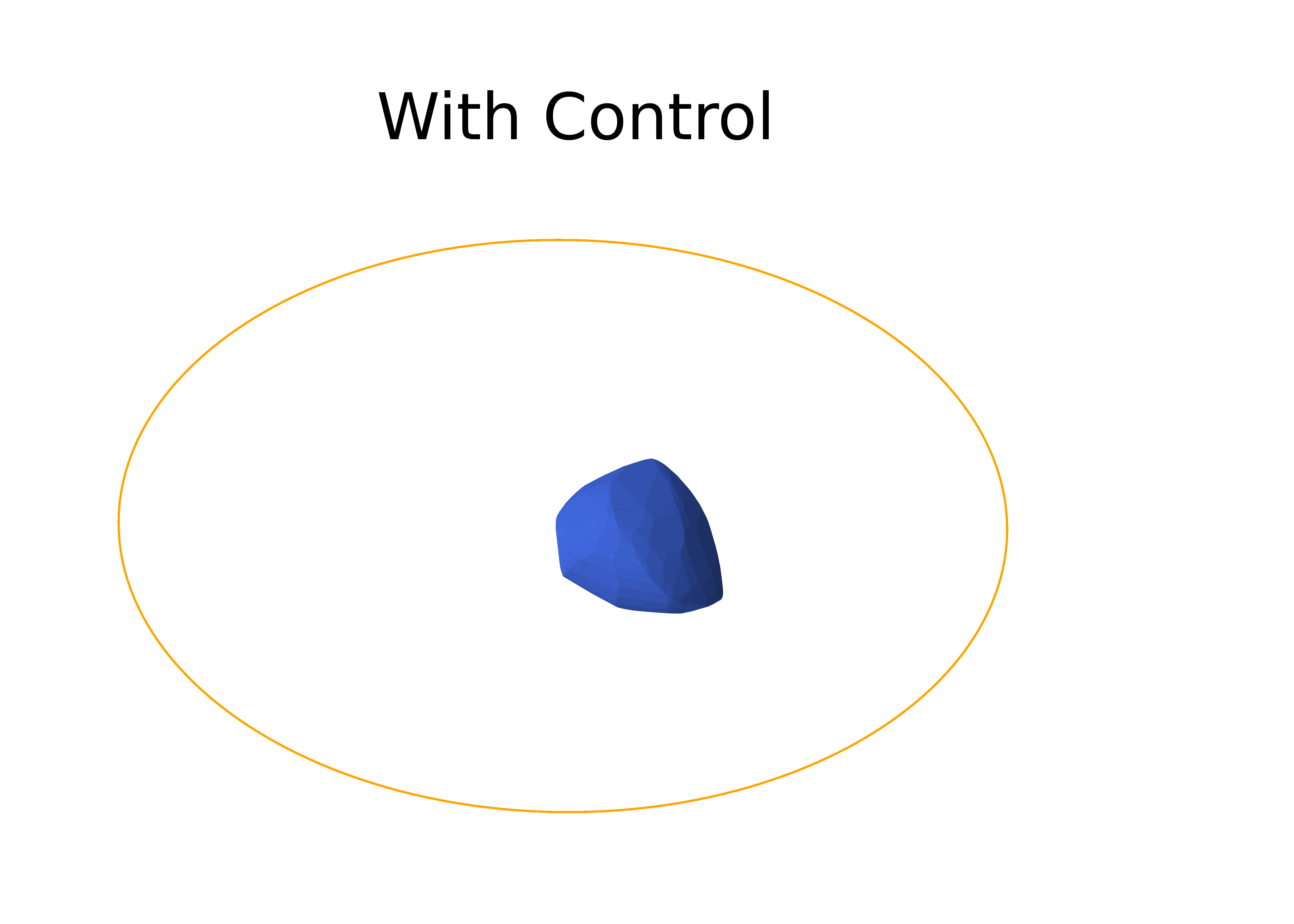
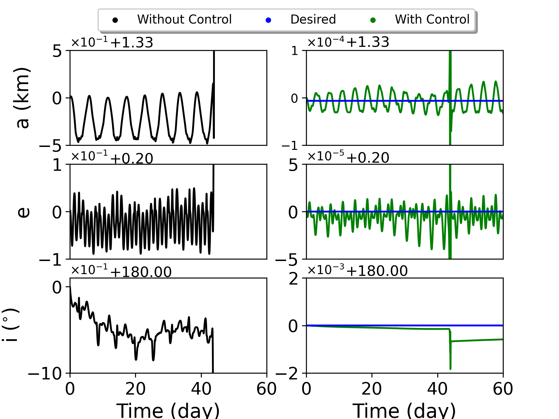
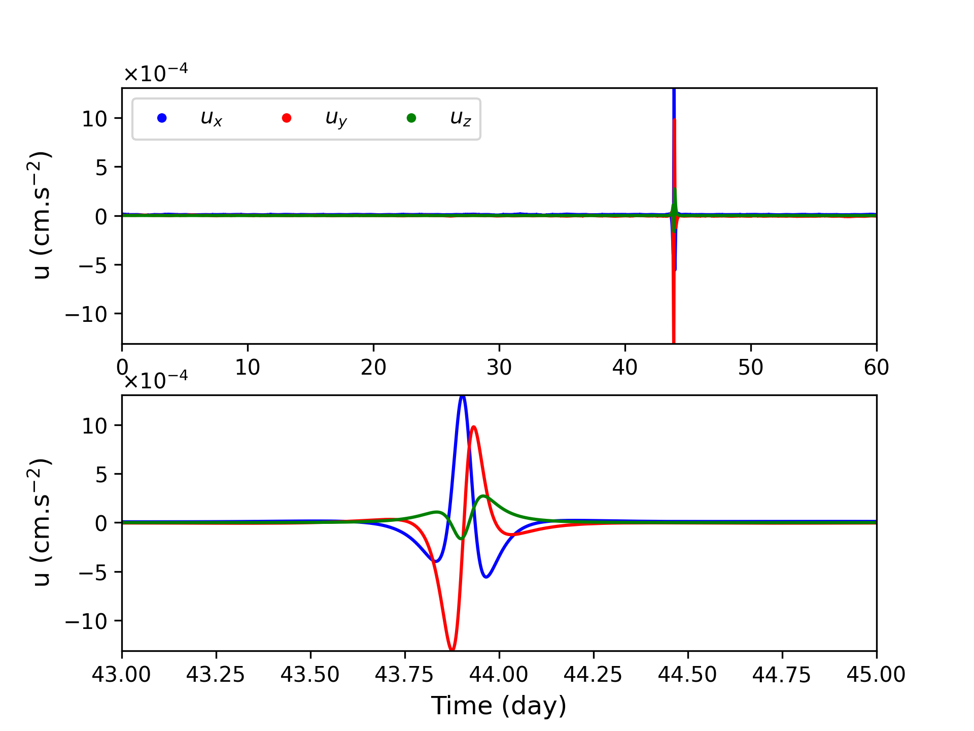
To demonstrate the effectiveness of our control, we considered all the perturbations (as mentioned in Sec. 4 above) on a spacecraft in an orbit with an initial semimajor axis of 1.325 km, initial eccentricity of 0.2 and initial inclination of 180^∘ while the other orbital elements are fixed to 0. In Fig. 19 we present the orbit with (right-hand side) and without (left-hand side) control. The spacecraft without control will escape Apophis in 43 days, just after the close approach with our planet. However, our control, with a desired orbital parameters are the same as the initial ones, successfully stabilizing this orbit with a total $\bigtriangleup V$ of 0.495 m/s for 60 days of operation, which is a very law value. One can notice satisfactory small deviations from the reference orbit with a single peak in the controlled orbital elements, which corresponds to the moment of the close approach with Earth, where the components of the control input become larger and thus require more energy, as shown in Fig 20.

Figure 19: Controlled orbit close to (99942) Apophis, in the inertial frame. $a_{0}=0.5$ km, $e_{0}=0.2$, $i_{0}=180^{\circ}$, and other orbital parameters are fixed to 0.

Figure 20: The control components of the orbit shown in Fig. 19

7 CPM-Asteroid database

As a result of all our computations, we constructed the CPM-Asteroid (Close Proximity Motion relative to an Asteroid) database, which contains at its present extent the surfaces of section in the potential of (99942) Apophis in the body-fixed frame of reference, distributing our initial conditions in the x- and y-axis, which are related to symmetry. We considered 50 values of $H$, varying from $0.1$ to $5.0\times 10^{-9}$. In parallel, we deliver for each orbit the corresponding tables giving the Fourier and Poisson series for the x-, y-, and z-coordinate. We used a web application framework developed with Shiny in R, and made our results available in the GitHub repository under an MIT public license. CPM-Asteroid is available in https://github.com/safwanaljbaae/CPM-Asteroid. Any other data presented in this paper can be obtained directly from the corresponding author upon reasonable request.

Conclusions

In this work, we have carried out a detailed study of the dynamics around the asteroid (99942) Apophis, one of the most interesting Near-Earth Asteroids due to its Earth close approach on April 13th.,2029. We tried to provide a preliminary realistic analysis of the orbit dynamics about the asteroid. Inspired by previous works on modeling the gravitational potential of nonspherical bodies, we calculated the mass of each tetrahedron of the (99942) Apophis shape and assigned it to a point mass in its center, representing our asteroid as a sum of 2024 points that correspond to the number of faces in the shape. That allows us to considerably reduce the computation processing time using other methods. As a preliminary step to propose an Apophis mission, we neglected, in this work, the effect of tumbling and the influence of the Earth’s tides on the spin state. This interaction is still completely unknown and out the scope of this work. We obtained the physical properties and analyzed the equilibria near our target considering only the effects of a uniformly rotating 2024 points gravity field. The surfaces of section are calculated in the potential of (99942) Apophis in the body-fixed frame to show the behaviors of large scale orbits considering or not the perturbations of the planets in our Solar System and the SRP, which can considerably affect the dynamics around our target. The close approach with our planet imposes a fast and relatively strong perturbation making the vast majority of the tested orbits collide or escape from the system. An OSIRIS-REx-like spacecraft is considered for numerical analysis of orbital dynamics associated with (99942) Apophis, considering the full perturbations on the system. We employed the Runge-Kutta 7/8 variable step-size algorithm covering a period of 60 days, starting from March 1, 2029. The initial state vector of the particles is calculated using the classical orbital parameters ($a$, $e$, $i$, $\varpi$, $w$, and $f$). The variations of the semimajor axis are used to identify the less perturbed region in the system. We can state that the region with initial semimajor axis smaller than 4 km and initial eccentricity smaller than 0.4 affected by relatively small perturbations before the close approach with our planet. However, there is no stable regions around our target during the close approach. We applied the sliding mode control theory in order to solve the stabilization problem for the system. With a total $\bigtriangleup V$ of 0.495 m/s for 60 days of operation, we successfully stabilized an orbit with an initial semimajor axis of 0.5 km. Finally, we argue that our computations in this work could be refined in the future by taking into account the changes of the spin axis and rate of (99942) Apophis during the 2029 close encounter with our planet. Nevertheless, we estimate that our work provids a resonable approach of dynamical analysis of future spacecraft missions related to the target. It will be even very difficult, from a ballistic point of view, to launch a probe close to (99942) Apophis, but the idea deserves some interest.

8 acknowledgements

The authors would like to thank the Coordination for the Improvement of Higher Education Personnel (CAPES), which supported this work via the grant 88887.374148/2019-00, and the São Paulo State Science Foundation (FAPESP, grant 2017/20794-2). We are grateful to Dr. Wael Al Zoughbi, MD, PHD from the University of Weill Cornell Medicine for the discussions that motivated us to create the database CPM-Asteroid mentiond in this work.

Conflict of interest

The authors declare that they have no conflict of interest.

References

- Aljbaae (2013) Aljbaae S (2013) Effets des astéroïdes sur les mouvements orbitaux des planètes telluriques. PhD thesis, SYRTE, Paris Observatory
- Aljbaae and Souchay (2012) Aljbaae S, Souchay J (2012) Specific effects of large asteroids on the orbits of terrestrial planets and the ASETEP database. A&A540:A21, DOI 10.1051/0004-6361/201118564
- Aljbaae et al. (2017) Aljbaae S, Chanut TGG, Carruba V, Souchay J, Prado AFBA, Amarante A (2017) The dynamical environment of asteroid 21 Lutetia according to different internal models. MNRAS464:3552–3560, DOI 10.1093/mnras/stw2619, 1610.02338
- Aljbaae et al. (2019) Aljbaae S, Chanut TGG, Prado AFBA, Carruba V, Hussmann H, Souchay J, Sanchez DM (2019) Orbital stability near the (87) Sylvia system. MNRAS486:2557–2569, DOI 10.1093/mnras/stz998
- Aljbaae et al. (2020) Aljbaae S, Prado AFBA, Sanchez DM, Hussmann H (2020) Analysis of the orbital stability close to the binary asteroid (90) Antiope. MNRAS496(2):1645–1654, DOI 10.1093/mnras/staa1634
- Bancelin et al. (2012) Bancelin D, Colas F, Thuillot W, Hestroffer D, Assafin M (2012) Asteroid (99942) Apophis: new predictions of Earth encounters for this potentially hazardous asteroid. A&A544:A15, DOI 10.1051/0004-6361/201117981
- Beutler (2005) Beutler G (2005) Methods of celestial mechanics. Vol. II: Application to planetary system geodynamics and satellite geodesy
- Borderes-Motta and Winter (2018) Borderes-Motta G, Winter OC (2018) Poincaré surfaces of section around a 3D irregular body: the case of asteroid 4179 Toutatis. MNRAS474(2):2452–2466, DOI 10.1093/mnras/stx2958, 1711.06506
- Bottke et al. (2006) Bottke WF, Vokrouhlický D, Rubincam DP, Nesvorný D (2006) The yarkovsky and yorp effects: Implications for asteroid dynamics. Annual Review of Earth and Planetary Sciences 34(1):157–191, DOI 10.1146/annurev.earth.34.031405.125154, URL https://doi.org/10.1146/annurev.earth.34.031405.125154, https://doi.org/10.1146/annurev.earth.34.031405.125154
- Brozović et al. (2018) Brozović M, Benner LAM, McMichael JG, et al (2018) Goldstone and Arecibo radar observations of (99942) Apophis in 2012-2013. Icarus300:115–128, DOI 10.1016/j.icarus.2017.08.032
- Chanut et al. (2015a) Chanut TGG, Aljbaae S, Carruba V (2015a) Mascon gravitation model using a shaped polyhedral source. MNRAS450:3742–3749, DOI 10.1093/mnras/stv845
- Chanut et al. (2015b) Chanut TGG, Winter OC, Amarante A, Araújo NCS (2015b) 3D plausible orbital stability close to asteroid (216) Kleopatra. MNRAS452(2):1316–1327, DOI 10.1093/mnras/stv1383
- Chanut et al. (2017) Chanut TGG, Aljbaae S, Prado AFBA, Carruba V (2017) Dynamics in the vicinity of (101955) Bennu: solar radiation pressure effects in equatorial orbits. MNRAS470:2687–2701, DOI 10.1093/mnras/stx1204, 1705.09564
- Chesley et al. (2009) Chesley SR, Milani A, Tholen D, Bernardi F, Chodas P, Micheli M (2009) An Updated Assessment Of The Impact Threat From 99942 Apophis. In: AAS/Division for Planetary Sciences Meeting Abstracts #41, AAS/Division for Planetary Sciences Meeting Abstracts, p 43.06
- Descamps et al. (2011) Descamps P, Marchis F, Berthier J, Emery ea (2011) Triplicity and physical characteristics of Asteroid (216) Kleopatra. Icarus211:1022–1033, DOI 10.1016/j.icarus.2010.11.016, 1011.5263
- Durech et al. (2010) Durech J, Sidorin V, Kaasalainen M (2010) DAMIT: a database of asteroid models. A&A513:A46, DOI 10.1051/0004-6361/200912693
- Gastineau and Laskar (2011) Gastineau M, Laskar J (2011) Trip: A computer algebra system dedicated to celestial mechanics and perturbation series. ACM Commun Comput Algebra 44(3/4):194–197, DOI 10.1145/1940475.1940518, URL http://doi.acm.org/10.1145/1940475.1940518
- Giorgini et al. (2008) Giorgini JD, Benner LAM, Ostro SJ, Nolan MC, Busch MW (2008) Predicting the Earth encounters of (99942) Apophis. Icarus193(1):1–19, DOI 10.1016/j.icarus.2007.09.012
- Hanuš et al. (2017) Hanuš J, Viikinkoski M, Marchis F, Ďurech J, Kaasalainen M, Delbo’ M, Herald D, Frappa E, Hayamizu T, Kerr S, Preston S, Timerson B, Dunham D, Talbot J (2017) Volumes and bulk densities of forty asteroids from ADAM shape modeling. A&A601:A114, DOI 10.1051/0004-6361/201629956, 1702.01996
- Jiang et al. (2014) Jiang Y, Baoyin H, Li J, Li H (2014) Orbits and manifolds near the equilibrium points around a rotating asteroid. Ap&SS349:83–106, DOI 10.1007/s10509-013-1618-8, 1403.0401
- Jiang et al. (2016) Jiang Y, Baoyin H, Wang X, Yu Y, Li H, Peng C, Zhang Z (2016) Order and chaos near equilibrium points in the potential of rotating highly irregular-shaped celestial bodies. Nonlinear Dynamics 83(1):231–252, DOI 10.1007/s11071-015-2322-8, URL https://doi.org/10.1007/s11071-015-2322-8
- Kinoshita and Nakai (1991) Kinoshita H, Nakai H (1991) Secular Perturbations of Fictitious Satellites of Uranus. Celestial Mechanics and Dynamical Astronomy 52(3):293–303, DOI 10.1007/BF00048489
- Lowry et al. (2014) Lowry SC, Weissman PR, Duddy SR, Rozitis B, Fitzsimmons A, Green SF, Hicks MD, Snodgrass C, Wolters SD, Chesley SR, Pittichová J, van Oers P (2014) The internal structure of asteroid (25143) Itokawa as revealed by detection of YORP spin-up. A&A562:A48, DOI 10.1051/0004-6361/201322602
- Mirtich (1996) Mirtich B (1996) Fast and accurate computation of polyhedral mass properties. Journal of graphics tools 1
- Müller et al. (2014) Müller TG, Kiss C, Scheirich P, Pravec P, O’Rourke L, Vilenius E, Altieri B (2014) Thermal infrared observations of asteroid (99942) Apophis with Herschel. A&A566:A22, DOI 10.1051/0004-6361/201423841, 1404.5847
- Negri and Prado (2020a) Negri RB, Prado AFBA (2020a) A Novel Robust 3-D Path Following Control for Keplerian Orbits. Submitted to Automatica
- Negri and Prado (2020b) Negri RB, Prado AFBA (2020b) Autonomous and Robust Orbit Keeping for Small Body Missions. Submited to Journal of Guidance, Control, and Dynamics
- Pravec et al. (2014) Pravec P, Scheirich P, Ďurech J, et al (2014) The tumbling spin state of (99942) Apophis. Icarus233:48–60, DOI 10.1016/j.icarus.2014.01.026
- Sanchez and Prado (2017) Sanchez DM, Prado AFBA (2017) On the Use of Mean Motion Resonances to Explore the Haumea System. AAS/AIAA Astrodynamics Specialist Conference 162:1507–1524
- Sanchez and Prado (2019) Sanchez DM, Prado AFBA (2019) Searching for Less-Disturbed Orbital Regions Around the Near-Earth Asteroid 2001 SN263. Journal of Spacecraft and Rockets 56(6):1775–1785, DOI 10.2514/1.A34402
- Sanchez et al. (2014) Sanchez DM, Prado AFBA, Yokoyama T (2014) On the effects of each term of the geopotential perturbation along the time I: Quasi-circular orbits. Advances in Space Research 54:1008–1018, DOI 10.1016/j.asr.2014.06.003
- Sansaturio and Arratia (2008) Sansaturio ME, Arratia O (2008) Apophis: the Story Behind the Scenes. Earth Moon and Planets 102(1-4):425–434, DOI 10.1007/s11038-007-9165-3
- Scheeres et al. (2005) Scheeres D, Benner L, Ostro S, Rossi A, Marzari F, Washabaugh P (2005) Abrupt alteration of asteroid 2004 mn4’s spin state during its 2029 earth flyby. Icarus 178(1):281 – 283, DOI https://doi.org/10.1016/j.icarus.2005.06.002, URL http://www.sciencedirect.com/science/article/pii/S0019103505002174
- Scheeres (1994) Scheeres DJ (1994) Dynamics about uniformly rotating triaxial ellipsoids: Applications to asteroids. Icarus110:225–238, DOI 10.1006/icar.1994.1118
- Scheeres et al. (1998) Scheeres DJ, Ostro SJ, Hudson RS, DeJong EM, Suzuki S (1998) Dynamics of Orbits Close to Asteroid 4179 Toutatis. Icarus132(1):53–79, DOI 10.1006/icar.1997.5870
- Scheeres et al. (2000) Scheeres DJ, Williams BG, Miller JK (2000) Evaluation of the Dynamic Environment of an Asteroid: Applications to 433 Eros. Journal of Guidance Control Dynamics 23:466–475, DOI 10.2514/2.4552
- Smalley et al. (2005) Smalley KE, Garradd GJ, Benner LAM, Nolan MC, Giorgini JD, Chesley SR, Ostro SJ, Scheeres DJ (2005) 2004 MN_4. IAU Circ.8477:1
- Souchay et al. (2014) Souchay J, Souami D, Lhotka C, Puente V, Folgueira M (2014) Rotational changes of the asteroid 99942 Apophis during the 2029 close encounter with Earth. A&A563:A24, DOI 10.1051/0004-6361/201322364
- Souchay et al. (2018) Souchay J, Lhotka C, Heron G, Hervé Y, Puente V, Folgueira Lopez M (2018) Changes of spin axis and rate of the asteroid (99942) Apophis during the 2029 close encounter with Earth: A constrained model. A&A617:A74, DOI 10.1051/0004-6361/201832914
- Tsoulis and Petrović (2001) Tsoulis D, Petrović S (2001) On the singularities of the gravity field of a homogeneous polyhedral body. Geophysics 66(2):535, DOI 10.1190/1.1444944
- Venditti (2013) Venditti FCF (2013) Manobras orbitais ao redor de corpos irregulares. PhD thesis, INPE, São José dos Campos
- Wang et al. (2014) Wang X, Jiang Y, Gong S (2014) Analysis of the potential field and equilibrium points of irregular-shaped minor celestial bodies. Ap&SS353:105–121, DOI 10.1007/s10509-014-2022-8, 1403.5025
- Werner (1997) Werner RA (1997) Spherical harmonic coefficients for the potential of a constant-density polyhedron. Computers and Geosciences 23:1071–1077, DOI 10.1016/S0098-3004(97)00110-6
- Yu and Baoyin (2012) Yu Y, Baoyin H (2012) Orbital Dynamics in the Vicinity of Asteroid 216 Kleopatra. AJ143(3):62, DOI 10.1088/0004-6256/143/3/62