The dynamical environment of asteroid 21 Lutetia
according to different internal models

Abstract

One of the most accurate models currently used to represent the gravity field of irregular bodies is the polyhedral approach. In this model, the mass of the body is assumed to be homogeneous, which may not be true for a real object. The main goal of the present paper is to study the dynamical effects induced by three different internal structures (uniform, three- and four-layers) of asteroid (21) Lutetia, an object that recent results from space probe suggest being at least partially differentiated. The Mascon gravity approach used in the present work, consists of dividing each tetrahedron into eight parts to calculate the gravitational field around the asteroid. The zero-velocity curves show that the greatest displacement of the equilibrium points occurs in the position of the E4 point for the four-layers structure and the smallest one occurs in the position of the E3 point for the three-layers structure. Moreover, stability against impact shows that the planar limit gets slightly closer to the body with the four-layered structure.

We then investigated the stability of orbital motion in the equatorial plane of (21) Lutetia and propose numerical stability criteria to map the region of stable motions. Layered structures could stabilize orbits that were unstable in the homogeneous model.

1 Introduction

The main challenge for the navigators of space missions to small irregular bodies is to derive pre-mission plans for the control of the orbits. A lot of studies have already been focused on this issue (Scheeres, 1994; Scheeres et al., 1998a, b; Rossi, Marzari, & Farinella, 1999; Hu, 2002). Generally, the potential of an asteroid can be estimated from its shape assuming a homogeneous density distribution. Yet, it remains an approximation to reality, since real bodies are affected by density irregularities. Therefore, it seems worthwhile to discuss the effects of different mass distributions of objects on their gravity field and, consequently, on their orbital environment. For instance, several studies modeled the gravitational forces of Ceres and Vesta by a spherical harmonic expansion assuming diverse scenarios for interior structure (Tricarico & Sykes, 2010; Konopliv et al., 2011, 2014; Park et al., 2014). In addition, the polyhedral approach (Werner & Scheeres, 1997) seems more appropriate for evaluating the gravitational forces close to the surface. The main problem of these approaches is the heavy computation time of the integrations. This issue has been recently reported in Chanut, Aljbaae, & Carruba (2015a) in developing a new approach that models the external gravitational field of irregular bodies through mascons. The authors applied the mascon gravity framework using a shaped polyhedral source, dividing each tetrahedron into up to three parts. That drives the attention to the possibility of taking into consideration the structure of layers in the gravitational potential computation.

The asteroid (21) Lutetia belongs to the main belt, the orbital space between Mars and Jupiter. An analysis of its surface composition and temperature, Coradini et al. (2011) showed that Lutetia was likely formed during the very early phases of the Solar System. Moreover, measurements by the European Space Agency’s Rosetta have found that this asteroid was unusually dense for an asteroid ($3.4~{}g\cdot cm^{-3}$). Its large density suggests that the asteroid might be a partially differentiated body, with a dense metal-rich core (Pätzold et al., 2011; Weiss et al., 2012). For these reasons, (21) Lutetia represents a suitable object to test the effects of the layers structure on the gravity field.

Thus, this paper aims at computing the gravitational field associated with asteroid (21) Lutetia, considering a model with different density layers. Moreover, we mapped the orbital dynamics of a probe-target close to it, taking into account this in-homogeneous model. For these purposes, first the physical properties of the polyhedral shape of (21) Lutetia are presented in section 2. Then, two models with different internal structures (three- and four-layers) are discussed in section 3. Moreover, the dynamical properties in the vicinity of our target are studied in section 4. Here we calculated the Jacobi integral and obtained the zero-velocity surfaces and the particular solutions of the system. A numerical analysis of the stability of motions in the equatorial plane is presented in section 5. Finally, the main results of our study are given in section 6.

2 Physical properties from the polyhedral shape of Lutetia with uniform density

The relatively large asteroid (21) Lutetia is a primordial object, located in the inner part of the main-belt, with a perihelion of 2.036 AU and an aphelion distance of 2.834 AU. Its eccentricity (0.164) is moderate, and its inclination with respect to the ecliptical plane is quite small (3.0648^∘) (Schulz et al., 2010). The asteroid was encountered by Rosetta spacecraft on its way to its final target (the comet 67P/Churyumov-Gerasimenko), at a distance of $3168\pm 7.5$ $km$ and a relative fly-by velocity of 14.99 $km.s^{-1}$. The asteroid’s mass was estimated by the gravitational field distortion of the flyby trajectory measured by the Doppler shift of the radio signals from Rosetta as $(1.7\pm 0.017)\times 10^{18}~{}kg$,. It is lower than the previous estimation of $(2.59\pm 0.24)\times 10^{18}~{}kg$ obtained from asteroid to asteroid perturbations (Pätzold et al., 2011). Its bulk density of $3.4\pm 0.3~{}g.cm^{-3}$ was calculated using the volume determined by the Rosetta Optical, Spectroscopic, and Infrared Remote Imaging System (OSIRIS) camera. This density is close to the density of M-type asteroids like (216) Kleopatra (Descamps et al., 2011).

Sierks et al. (2011) have modeled a global shape of (21) Lutetia, combining two techniques: stereo-photoclinometry (Gaskell et al., 2008) using images obtained by OSIRIS, and inversion of a set of 50 photometric light curves and contours of adaptive optics images (Carry et al., 2010; Kaasalainen, 2011). Twelve different shape model solutions are listed in the Planetary Data System (PDS).

In this work we selected the shape model that has 2962 faces from the PDS database. The body is aligned with the principal axes of inertia, in such a way that the inertia tensor becomes a diagonal matrix. Thus, the x-axis is aligned with the smallest moment of inertia (longest axis), while the z-axis is aligned with the largest (shortest axis), and the y-axis is aligned with the intermediate one. The spin velocity of (21) Lutetia is assumed to be uniform around its maximum moment of inertia ($z$ axis) with a period of $8.168270\pm 0.000001$ hours (Carry et al., 2010). The algorithm of Werner (1997) was used to calculate the spherical harmonic coefficients $C_{n,m}$ and $S_{n,m}$ up to degree 4 (Table 1), considering a uniform bulk density of $3.4~{}g.cm^{-3}$. Please notice that these coefficients are presented as a reference for describing the exterior gravitational potential. They can be used to verify the orientation of our shape. If we fix the expansion of the gravitational field around the center of mass, we have C 11 = S 11 = 0, and if the axes are exactly oriented along the principal axes of inertia, we have C21 = S 21 = S 22 = 0 (Scheeres, Williams, & Miller, 2000). However, we did not use these coefficients in our analyses, our approach (mascon) employs the shape of the asteroid to calculate the exterior gravitational potential, which is more accurate than the harmonic coefficients even if this coefficients were measured up to a higher degree than four.

The algorithm of Mirtich (1996) provides these values of moments of inertia divided by the total mass of the body:

$$I_{xx}/M = 802.929~{}~{}km^{2}$$

$$I_{yy}/M = 1096.555~{}~{}km^{2}$$

$$I_{zz}/M = 1263.996~{}~{}km^{2}$$

From the moments of inertia, we can solve for the equivalent ellipsoid according to Dobrovolskis (1996). The semi-major axes found are: $62.402\times 49.254\times 39.859$ km

As discussed by Hu & Scheeres (2004), the main gravity coefficients are directly related to the principal moments of inertia (normalized by the body mass) and the unit is the distance squared.

$$C_{20} = -\frac{1}{2M}(2I_{zz}-I_{xx}-I_{yy})=-314.254\,km^{2}$$

$$C_{22} = \frac{1}{4M}(I_{yy}-I_{xx})=73.406\,km^{2}$$

A mass-distribution parameter $\sigma$ can determined to be:

$$\sigma=\frac{I_{yy}-I_{xx}}{I_{zz}-I_{xx}}=-\frac{4C_{22}}{C_{20}-2C_{22}}=0.637$$

this value of $\sigma$ denotes that Lutetia is not close to the rotational symmetry about the z-axis ($\sigma=0$) or x-axis ($\sigma=1$). That clearly appears in the elongated shapes viewed from various perspectives presented in Fig. 1, with overall dimensions ($km$) of $(-66.854,57.959)\times(-54.395,47.920)\times(-44.238,39.721)$ in the x,y, and z directions, respectively, and a polyhedral volume of $495140.993~{}km^{3}$ (volume-equivalent diameter of 98.155 $km$).

Table 1: Lutetia Gravity Field Coefficients up to order 4, using the shape model of 2962 faces. These coefficients are computed with respect to a constant density of 3.4 $g.cm^{-3}$, a total mass of 1.68 $\times 10^{18}$ kg (derived from the polyhedron volume), and a reference distance of 49.1 km.

Order	Degree	$C_{nm}$	$S_{nm}$
0	0	1.0000000000	-
1	0	-2.4161445414 $\times 10^{-16}$	-
1	1	4.4587814343 $\times 10^{-17}$	7.2140102052 $\times 10^{-17}$
2	0	-1.3047303671 $\times 10^{-1}$	-
2	1	2.0156673639 $\times 10^{-16}$	8.9487336812 $\times 10^{-17}$
2	2	3.0477066056 $\times 10^{-2}$	8.6521705057 $\times 10^{-16}$
3	0	-8.1225875136 $\times 10^{-3}$	-
3	1	1.3607877846 $\times 10^{-2}$	6.4377447088 $\times 10^{-3}$
3	2	1.7536608648 $\times 10^{-5}$	-3.1776398240 $\times 10^{-4}$
3	3	-2.3473257023 $\times 10^{-3}$	1.5994949238 $\times 10^{-3}$
4	0	3.5318181727 $\times 10^{-2}$	-
4	1	8.1522038541 $\times 10^{-4}$	-4.7670141468 $\times 10^{-3}$
4	2	-2.4926821394 $\times 10^{-3}$	1.3305167431 $\times 10^{-3}$
4	3	3.8256764962 $\times 10^{-5}$	4.5914129725 $\times 10^{-4}$

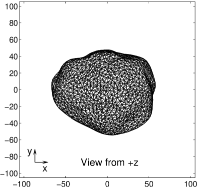
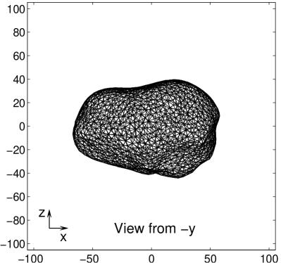
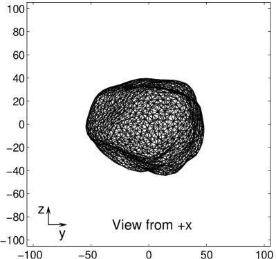
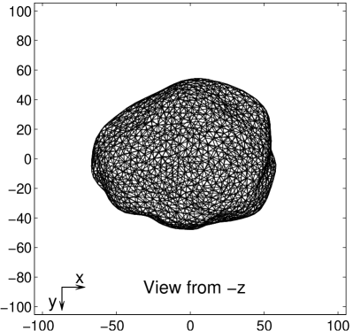
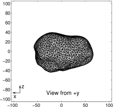
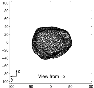
Figure 1: Polyhedral shape of (21) Lutetia shown in 6 perspective views ($\pm$ x, $\pm$ y, and $\pm$ z), using the shape model provided by PDS database with 2962 triangular faces (Sierks et al., 2011), after aligning the asteroid with the principal axes of inertia.

3 Internal structure of Lutetia

Because of its high IRAS albedo of $0.208\pm 0.025$, (21) Lutetia was classified as M-type asteroid by Barucci et al. (1987) and Tholen (1989). Analyzing the visible spectrum, Bus & Binzel (2002) classified it as (Xk) on the basis of SMASS II spectroscopic data. Further spectroscopic observations by Birlan et al. (2004); Barucci et al. (2005); Lazzarin et al. (2004, 2009) suggested a similarity with the carbonaceous chondrite spectra that characterize the C-type asteroids. Analyzing the reflectance spectra, Busarev et al. (2004) indicated the possibility of Lutetia being an M-type body covered with irregular layer of hydrated silicates. The Bus-DeMeo taxonomy of asteroids (DeMeo et al., 2009) put Lutetia in the Xc subclass. Moreover, the available data from ROSETTA OSIRIS images has been analyzed by Magrin et al. (2012) and compared consistently with ground based observations, but no further deep analysis was possible, since Rosetta only made a relatively brief observation covering about 50% of the surface.

According to Neumann, Breuer, & Spohn (2013), (21) Lutetia may have a differentiated interior, i.e., an iron-rich core and a silicate mantle. Notice that the other differentiated asteroid such as (1) Ceres and (4) Vesta have been visited by a spacecraft (DAWN). Because of its large diameter, we think that it is reasonable to expect an internal differentiated structure for (21) Lutetia as well. To understand the effects that such differentiation may have on the orbits of probes, we will study the dynamics in the vicinity of (21) Lutetia examining the effect of its in-homogeneity, considering two distinct models, based on a three-layers and a four-layers assumption, respectively, as already used for other differentiated objects.

3.1 The three-layers internal model

Our three-layers model is similar to that discussed in Park et al. (2014) and Konopliv et al. (2014). It corresponds to a volume-equivalent diameter of 98.155 $km$, in which a crust with a mean thickness of 18.404 $km$ occupies 75.59% of the total volume with a density of 3.2 $g.cm^{-3}$, that represents 71.06% of the total mass. The mantle thickness of the asteroid is also modeled with a 18.404 $km$ thickness (22.85% of the total volume) and a density of 3.8 $g.cm^{-3}$ (25.54% of the total mass). The core, based on iron meteorites characteristics, is considered with a 12.27 $km$ thickness (1.56% of the total volume) and a density of 7.4 $g.cm^{-3}$ (3.4% of the total mass). This structure is exhibited in Figure 2.

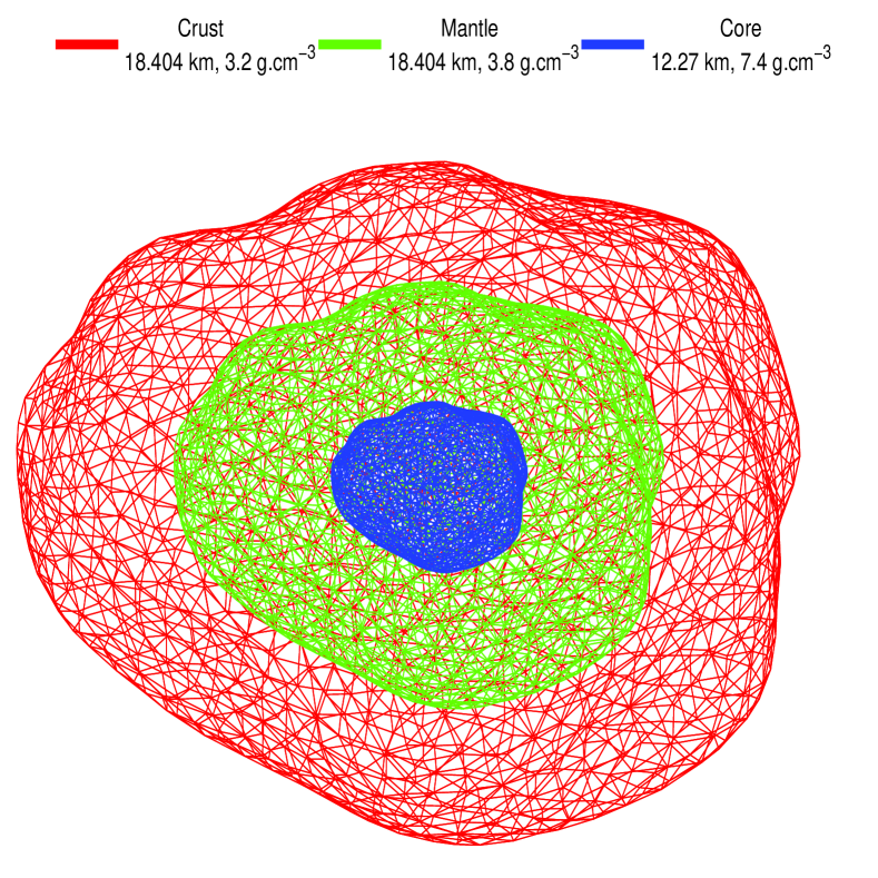
Figure 2: Three-layer structure of (21) Lutetia.

3.2 The four-layers internal model

A more sophisticated model of the internal structure of (21) Lutetia can be based on the model of Vesta discussed in Zuber et al. (2011). It consists in four layers, shown in Figure 3. This model still includes an iron meteorite core with a thickness of 18.404 $km$ (5.27% of the total volume) and a density of 7.8 $g.cm^{-3}$ (12.1% of the total mass). The mantle thickness is supposed to be 12.27 $km$ (19.15 % of the total volume) with a density of 4.0 $g.cm^{-3}$ (22.52% of the total mass). In that specific model the crust itself is divided into an upper and lower layers with limits at respectively 12.27 $km$ and 6,13 $km$ thickness. The upper crust represents 57.81% of the total volume with a density of 2.86 $g.cm^{-3}$ (48.66% of the total mass), whereas the lower crust represents 17.77% of the total volume with a density of 3.2 $g.cm^{-3}$ (16.72% of the total mass).

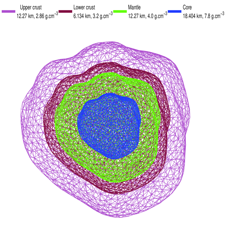
Figure 3: Four-layer structure of (21) Lutetia.

The two internal structures proposed for (21) Lutetia are summarized in Table 2. The layers size and density are constrained to the model of internal structures of Vesta discussed in Park et al. (2014); Konopliv et al. (2014) and Zuber et al. (2011). We preserve the total mass of Lutetia by fixing the medium density at $3.4~{}g.cm^{-3}$. In other words, the distribution of the gravity of Lutetia is changed in the three- and four-layers models to be greater at the center, while the mean density is the same as in the uniform structure.

Table 2: Three- and Four-layered structure of (21) Lutetia

	Thickness	Density	Volume	Mass
	($km$)	($g.cm^{-3}$)	(% of the total volume)	(% of the total mass)
Three-layer model
Core	12.270	7.40	1.56	3.40
Mantle	18.404	3.80	22.85	25.54
Crust	18.404	3.20	75.59	71.06
Four-layer model
Core	18.404	7.80	5.27	12.10
Mantle	12.27	4.00	19.15	22.52
Lower Crust	6.13	3.20	17.77	16.72
Upper Crust	12.27	2.86	57.81	48.66

3.3 Influence of the internal models on the gravitational potential

For assessing the effects of the two different internal structures above described on the external potential of (21) Lutetia, we used the shape model with 2962 triangular faces and applied the approach of Chanut, Aljbaae, & Carruba (2015a), dividing each tetrahedron into up to eight parts (Mascon 8), to at 980396 points placed in an equally spaced grid generated from the surface of the asteroid up to 200 km in the (x,y) plane. Mascon 8 seems to be satisfactory in terms of precision and computational time. Higher divisions could provide somewhat better accuracy but at a heavier computational cost.

Also, using the shape of the asteroid to model the external gravitational field according to the equation 9 in this paper or the equation 4 in Chanut, Aljbaae, & Carruba (2015a) is actually more accurate. According to Park et al. (2014), the spherical harmonic series may not converge close the surface but the polyhedral approach is guaranteed to converge outside of the polyhedron.

In Fig. 4 (left-hand side) we present the relative difference of the gravitational potential considering an uniform density $U_{M1}$ with the four-layers structure (red dots) or the three-layers structure (black dots). The figure shows that the relative difference is inversely proportional to the distance from the surface of the asteroid, and the potential calculated near the surface is affected significantly by the internal structure. Moreover, the shape model with 11954 triangular faces is also used in this work to calculate the same relative difference, and presented in Fig. 4 (right-hand side). A very good agreement between the two shapes was found. In terms of CPU time, the total simulation time on a Pentium 3.8 GHz CPU took about 16 minutes using the first shape model, while required 54 minutes with the second one. That guided us to use the model with 2962 faces for the rest of this work.

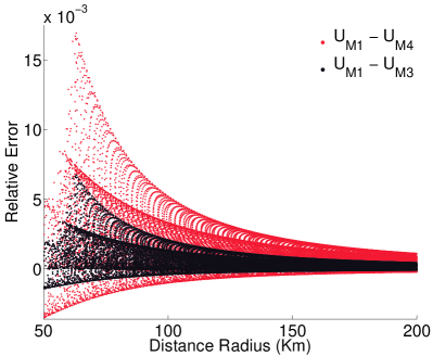
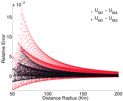
Figure 4: Relative difference of the gravitational potential calculated with Mascon 8 considering a uniform density $U_{M1}$ with the model, considering a four-layers structure (red dots) or a three-layers structure (black dots), using the shape model with 11954 triangular faces (left-hand side) and the shape model with 2962 triangular faces (right-hand side).

4 Equations of motion and dynamical properties in the vicinity of Lutetia

In this section, we evaluate the dynamical environment close to (21) Lutetia caused by its in-homogeneous structure, and its consequences on any spacecraft orbiting around it. First, we consider a zone where the effect of the solar gravity is considerably smaller than the asteroid gravity, that is to say a region inside its Hill sphere. Its Hill radius $R_{H}=r\sqrt[3]{\frac{m}{3M_{\text{\hbox{$\odot$}}}}}$ varies between 20042 $km$ at perihelion $(r_{p})$ and 27897 $km$ at aphelion $(r_{a})$. As an example, within 300 km from the asteroid center of mass, the solar gravity perturbation reaches $1.43\times 10^{-12}~{}m.s^{-2}$ at perihelion and $7.38\times 10^{-13}~{}m.s^{-2}$ at aphelion. That is completely negligible compared with the total gravitational attraction exercised by the asteroid on the spacecraft, which is $1.26\times 10^{-6}km.s^{-2}$.

Another perturbation that arises from the Sun is the Solar radiation pressure (SRP). Generally, the magnitude of the SRP acceleration ($g$) appears in the Hill equation of motion as a linear term in the first integral (Scheeres & Marzari, 2002). Assuming that the spacecraft is a flat plate oriented to the Sun, the SRP acceleration $g$ always acts in the anti-solar direction. It is computed as:

$$g=\frac{\beta}{d^{2}},$$ (1)

where $\beta=\frac{(1+\eta)G1}{B}$ is the SRP parameter, $G1=1\times 10^{8}kg.km^{3}s^{-2}m^{-2}$ is the solar constant (Giancotti et al., 2014), $\eta$ is the reflectance of the spacecraft material (equal to 0 for perfectly absorbing material and to 1 for perfect reflection), $B$ is the spacecraft mass to area ratio in $kg.m^{-2}$ usually computed by dividing the total mass by the projected surface area of the spacecraft and $d$ is the heliocentric distance of the asteroid in $km$. Taking into account the physical characteristics of a Rosetta-like spacecraft, i.e. a maximum projected area of $65~{}m^{2}$ and a mass of $1400~{}kg$ (Scheeres et al., 1998a), the total solar radiation pressure acceleration varies from $2.58\times 10^{-17}~{}m.s^{-2}$ up to $5.00\times 10^{-17}~{}m.s^{-2}$ at the aphelion and perihelion distance from the Sun, respectively. After considering the above calculations, we neglect the effects of both the SRP and the solar gravity in our model.

4.1 Equations of motion

According to Scheeres et al. (1996); Scheeres (1999, 2012), in the absence of any solar perturbations, the equations of motion of a spacecraft orbiting a uniformly rotating asteroid and significantly far from any other celestial body are

$$\ddot{x}-2\omega\dot{y} = \omega^{2}x+U_{x}$$ (2)

$$\ddot{y}+2\omega\dot{x} = \omega^{2}y+U_{y}$$ (3)

$$\ddot{z} = U_{z}.$$ (4)

where $U_{x}$, $U_{y}$ and $U_{z}$ are the first-order partial derivatives of the potential $U(x,y,z)$ and $\omega$ is the spin rate of the asteroid.

Because Eqs. (2) to (4) are time invariant, the Jacobi constant exists as an additional integral of motion. The Jacobi integral for the equations of motion is conserved and is explicitly calculated as

$$C=\underbrace{\frac{1}{2}\omega^{2}(x^{2}+y^{2})+U(x,y,z)}_{\text{Modified potential}}-\underbrace{\frac{1}{2}(\dot{x}^{2}+\dot{y}^{2}+\dot{z}^{2})}_{\text{Kinetic energy}}$$ (5)

4.2 Zero velocity surfaces and equilibria

As shown in Eq. (5), the Jacobi integral is a relation between the possible position of the particle and the kinetic energy with respect to the rotating asteroid. If the particle’s velocity becomes zero, the zero-velocity surfaces are defined by

$$C=\frac{1}{2}\omega^{2}(x^{2}+y^{2})+U(x,y,z)=V(x,y,z)$$ (6)

where $V(x,y,z)$ is the Modified potential.

This equation defines zero-velocity surfaces depending on the asteroid shape and also on the value of $C$. These surfaces are all evaluated close to the critical values of $C$ and intersect or close in upon themselves at points called equilibrium points (Scheeres et al., 1996). The location of these equilibrium points can be found by solving the equation $\nabla V(x,y,z)=0$. The number of solutions depends on the shape and on the spin rate of the asteroid.

Using the shape model of (21) Lutetia with 2962 triangular faces, the projection of the zero-velocity surface onto the $z=0$ plane is shown in Figure 5. The zero-velocity curves of the asteroid have four solutions outside the body, separated by approximately $90^{\circ}$ in longitude. Only the external equilibria are presented in this work since there is not a good agreement between Mascon 8 and the classical polyhedron method inside the body. However, the agreement is better outside and near the body surface (Chanut, Aljbaae, & Carruba, 2015a).

Figs. 5 displays the results from the Mascon 8 model and the four-layers structure. Results for the classical polyhedral model, for the Mascon 8 gravity model with uniform density, and for the Mascon 8 with three-layers are similar and will not be displayed, for brevity. The maximum difference between the classical polyhedral approach and the Mascon 8 considering a uniform density occurs at the location of E4 (0.143 km, which represents 0.11% of the distance from the center of the body), and being less than the null hypothesis level, may therefore be considered satisfactory.

We observe that the positions of the equilibrium points (E1, E2, E3, E4) are moved by up to 0.112, 0.137, 0.0614, and 0.143 km considering the three-layers structure, and up to 0.294, 0.351, 0.173, and 0.417 km considering the four-layers one, respectively.

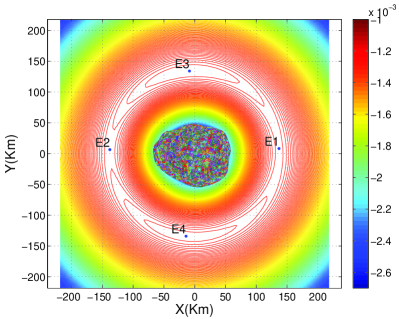
Figure 5: Zero-velocity curves and equilibrium points of (21) Lutetia in the xoy plane, obtained using the shape model with 2962 triangular faces and the four-layers structure. The colour code gives the intensity of the Jacobi constant in $km^{2}s^{−2}$. The equilibrium points outside the body ($E_{1},E_{2},E_{3},E_{4}$) are displayed in the figure.

Table 3: Locations of equilibrium points of (21) Lutetia and their Jacobi constant C (using the shape model of 2962 faces), generated by the classical polyhedral model (Tsoulis & Petrović, 2001) and the Mascon 8 gravity model (Chanut, Aljbaae, & Carruba, 2015a).

	x (km)	y (km)	z (km)	$C(km^{2}s^{-2}$)
Polyhedral model, uniform density
E1	137.10784172	8.44279347	0.08555291	-0.12634256 $\times 10^{-2}$
E2	-138.19144378	6.56551358	0.04185644	-0.12679936 $\times 10^{-2}$
E3	-8.70389476	134.01690523	0.03696436	-0.12441019 $\times 10^{-2}$
E4	-14.61831274	-134.06107222	0.08749509	-0.12467120 $\times 10^{-2}$
Mascon 8, uniform density
E1	137.08769819	8.38960864	0.09077155	-0.12632687 $\times 10^{-2}$
E2	-138.15024726	6.54070646	0.04488269	-0.12677495 $\times 10^{-2}$
E3	-8.66458628	134.02811212	0.03854483	-0.12441517 $\times 10^{-2}$
E4	-14.47666720	-134.07545174	0.09370561	-0.12467157 $\times 10^{-2}$
Mascon 8, three-layered structure
E1	136.99825452	8.32304070	0.08727020	-0.12626501 $\times 10^{-2}$
E2	-138.01547466	6.50802298	0.04322724	-0.12669215 $\times 10^{-2}$
E3	-8.61381286	134.06254558	0.03698190	-0.12443281 $\times 10^{-2}$
E4	-14.33458820	-134.09482376	0.08998671	-0.12467656 $\times 10^{-2}$
Mascon 8, four-layered structure
E1	136.86707031	8.19520730	0.08068557	-0.12617328 $\times 10^{-2}$
E2	-137.81293855	6.44518383	0.04046285	-0.12656817 $\times 10^{-2}$
E3	-8.51569913	134.11522533	0.03433857	-0.12445911 $\times 10^{-2}$
E4	-14.06158951	-134.12920961	0.08318837	-0.12468367 $\times 10^{-2}$

As reported in many previous studies (Szebehely, 1967; Scheeres, 1994; Murray & Dermott, 1999; Hu & Scheeres, 2008; Yu & Baoyin, 2012; Jiang et al., 2014; Wang, Jiang, & Gong, 2014), we can also examine the stability of the equilibria determined above. The linearized state equations in the neighborhood of the equilibrium points are summarized as

$$\ddot{X}-2\omega\dot{Y}+U_{xx}X+U_{xy}Y+U_{xz}Z = 0$$

$$\ddot{Y}+2\omega\dot{X}+U_{xy}X+U_{yy}Y+U_{xz}Z = 0$$ (7)

$$\ddot{Z}+U_{xz}X+U_{xz}Y+U_{zz}Z = 0$$

where $X=x-x_{L}$, $Y=y-y_{L}$,$Z=z-z_{L}$, and ($x_{L}$,$y_{L}$,$z_{L}$) denote the coordinates of the equilibrium point, $U_{\zeta\eta}=\frac{\partial^{2}U}{\partial\zeta\partial\eta}:\zeta,\eta=x,y,z$. The eigenvalues of the equation 7 are calculated by finding the roots of the characteristic equation at the equilibrium point.

$$\lambda^{6}+\alpha\lambda^{4}+\beta\lambda^{2}+\gamma=0$$ (8)

where $\lambda$ is the eigenvalues, $\alpha=U_{xx}+U_{yy}+U_{zz}+4\omega^{2}$, $\beta=U_{xx}U_{yy}+U_{yy}U_{zz}+U_{zz}U_{xx}-U_{xy}^{2}-U_{yz}^{2}-U_{xz}^{2}+4\omega^{2}U_{zz}$, $\gamma=U_{xx}U_{yy}U_{zz}+2U_{xy}U_{yz}U_{xz}-U_{xx}U_{yz}^{2}-U_{yy}U_{xz}^{2}-U_{zz}U_{xy}^{2}$. For more information, we recommend that interested readers review equation 14 in Jiang et al. (2014). The linearization method is applied using the classical polyhedral model and the Mascon 8 approach with uniform density and Mascon 8 gravity model considering the two multiple layers structures. This requires calculating the second derivatives of the potential that results in correcting the analytical form already presented in Chanut, Aljbaae, & Carruba (2015a) with the following expression:

$$U=\sum\limits_{i=1}^{n}\frac{\mu_{i}}{r_{i}} \Rightarrow U_{\zeta}=\sum\limits_{i=1}^{n}-\frac{\mu_{i}\zeta_{i}}{r_{i}^{3}}$$

$$\frac{\partial}{\partial\eta}(U_{\zeta}) = \sum\limits_{i=1}^{n}\bigg{[}-\frac{\mu_{i}}{r_{i}^{3}}\frac{\partial}{\partial\eta}(\zeta_{i})+\frac{3\mu_{i}\zeta_{i}\eta_{i}}{r_{i}^{5}}\bigg{]}$$ (9)

Eq. (7) leads to the second derivatives

$$U_{\zeta\zeta} = \sum\limits_{i=1}^{n}\bigg{[}-\frac{\mu_{i}}{r_{i}^{3}}+\frac{3\mu_{i}\zeta_{i}^{2}}{r_{i}^{5}}\bigg{]}$$

$$U_{\zeta\eta} = \sum\limits_{i=1}^{n}\bigg{[}\frac{3\mu_{i}\zeta_{i}\eta_{i}}{r_{i}^{5}}\bigg{]}$$ (10)

$$\zeta,\eta = x,y,z\text{ and }\zeta\neq\eta$$

where $r=\sqrt{x^{2}+y^{2}+z^{2}}$ represents the distance between the center of mass of each tetrahedron shaping the asteroid and the external point. The eigenvalues of the linearized system are listed in table 4. The classification of the equilibrium points defined in Jiang et al. (2014); Wang, Jiang, & Gong (2014) shows that E1 and E2 belong to Case 2 (two pairs of imaginary eigenvalues and one pair of real eigenvalues). As a consequence, the saddle equilibrium points are unstable, whereas E3 and E4 belong to Case 1 (purely imaginary eigenvalues), that leads to a linear stability of center equilibrium points. Thus, according to the classification originally proposed by Scheeres (1994), (21) Lutetia can be classified as a Type I asteroid . We can conclude that the effects of the two layer structures chosen on the stability of the equilibria are not determining.

Table 4: Eigenvalues of the coefficient matrix at the 4 external equilibrium points.

Eigenvalues	E1		E2		E3		E4
Tsoulis & Petrović (2001) considering the uniform density
	$\times 10^{-3}$		$10^{\times-3}$		$10^{\times-3}$		$\times 10^{-3}$
$\lambda_{1}$	0.220401	$i$	0.225039	$i$	0.215898	$i$	0.217647	$i$
$\lambda_{2}$	-0.220401	$i$	-0.225039	$i$	-0.215898	$i$	-0.217647	$i$
$\lambda_{3}$	0.217889	$i$	0.223367	$i$	0.186893	$i$	0.195130	$i$
$\lambda_{4}$	-0.217889	$i$	-0.223367	$i$	-0.186893	$i$	-0.195130	$i$
$\lambda_{5}$	-0.068854		-0.096044		0.098844	$i$	0.076583	$i$
$\lambda_{6}$	0.068854		0.096044		-0.098844	$i$	-0.076583	$i$
Mascon 8 considering the uniform densities
	$\times 10^{-3}$		$10^{\times-3}$		$10^{\times-3}$		$\times 10^{-3}$
$\lambda_{1}$	0.220329	$i$	0.224875	$i$	0.215878	$i$	0.217595	$i$
$\lambda_{2}$	-0.220329	$i$	-0.224875	$i$	-0.215878	$i$	-0.217595	$i$
$\lambda_{3}$	0.217873	$i$	0.223245	$i$	0.187309	$i$	0.195345	$i$
$\lambda_{4}$	-0.217873	$i$	-0.223245	$i$	-0.187309	$i$	-0.195345	$i$
$\lambda_{5}$	-0.068571		-0.095370		0.098100	$i$	0.076186	$i$
$\lambda_{6}$	0.068571		0.095370		-0.098100	$i$	-0.076186	$i$
Mascon 8 considering the three-layered structure
	$\times 10^{-3}$		$10^{\times-3}$		$10^{\times-3}$		$\times 10^{-3}$
$\lambda_{1}$	0.220074	$i$	0.224448	$i$	0.215787	$i$	0.217422	$i$
$\lambda_{2}$	-0.220074	$i$	-0.224448	$i$	-0.215787	$i$	-0.217422	$i$
$\lambda_{3}$	0.217726	$i$	0.222875	$i$	0.188941	$i$	0.196268	$i$
$\lambda_{4}$	-0.217726	$i$	-0.222875	$i$	-0.188941	$i$	-0.196268	$i$
$\lambda_{5}$	-0.067270		-0.093478		0.095128	$i$	0.074283	$i$
$\lambda_{6}$	0.067270		0.093478		-0.095128	$i$	-0.074283	$i$
Mascon 8 considering the four-layered structure
	$\times 10^{-3}$		$10^{\times-3}$		$10^{\times-3}$		$\times 10^{-3}$
$\lambda_{1}$	0.219691	$i$	0.223786	$i$	0.215654	$i$	0.217165	$i$
$\lambda_{2}$	-0.219691	$i$	-0.223786	$i$	-0.215654	$i$	-0.217165	$i$
$\lambda_{3}$	0.217510	$i$	0.222310	$i$	0.191206	$i$	0.197591	$i$
$\lambda_{4}$	-0.217510	$i$	-0.222310	$i$	-0.191206	$i$	-0.197591	$i$
$\lambda_{5}$	-0.065291		-0.090502		0.090804	$i$	0.071479	$i$
$\lambda_{6}$	0.065291		0.090502		-0.090804	$i$	-0.071479	$i$

5 Orbital stability about Lutetia

The goal of this section is to evaluate what should be the influence of Lutetia internal structure on the trajectory of a spacecraft in a close orbit. Thus we numerically investigate the perturbations on initially equatorial orbits. In particular, we focus our analysis on the effects of the layered structures on limiting stability against impacts, so as to help us choosing the limits for periapsis radius in our stability analysis.

5.1 Stability Against Impact

According to (Scheeres, Williams, & Miller, 2000; Chanut, Winter, & Tsuchida, 2014; Chanut et al., 2015b), the stability against impact is devoted to characterize the spacecraft dynamics, choosing initial conditions in such a way that the spacecraft stays in the outer portion of the zero-velocity curve, and the value of the Jacobi integral is smaller or equal to a specific value, corresponding to the minimum value of the Jacobi constant at the equilibrium point E2 listed in Table 3. A simple check in terms of osculating orbital elements (periapsis radius, eccentricity, and initial longitude) for an equatorial orbit is applied in order to determine the occurrence of an impact with the surface:

$$\frac{-\mu(1+e)}{2r_{p}}+W\sqrt{\mu r_{p}(1+e)}+U(r=r_{p},\lambda)+J_{0}=0$$ (11)

According to this last equation, the limits for the zones of stability against impact for Lutetia are shown in Figure 6. The initial orbits that do not undergo impact with Lutetia correspond to the right-hand side of the curves. We remark that the curves related to the classical polyhedral approach and the Mascon 8 gravity model assuming a uniform density can hardly be distinguished. On the contrary, the curves related to multiple layers structures are quite distinct and get closer to the surface which means that the non impacting zones are larger than in the case of uniform density. The eccentricities in this analysis are limited to 0.4 because orbits with high eccentricities have a small perihelion distance, which implies that the spacecraft will travel at a high relative velocity when encountering the asteroid, and that would make these orbits unpractical for a space mission. We also notice that the initial eccentricity is not a primary parameter in affecting the periapsis distance: the periapsis distance is moved from a little less than 160 km for $e=0.4$ to a little more than 175 km for $e=0$. Thus, studying the stability against impact leads to conclude that orbits must lie outside of 175 km from Lutetia to avoid an impact on the surface.

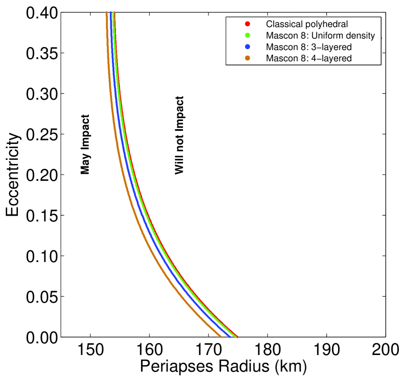
Figure 6: Stability against impact curve for equatorial, direct orbits around (21) Lutetia. The colours correspond to different approaches for calculating the potential : a classical polyhedral approach considering a uniform density and a Mascon 8 gravity model assuming the three- and four-layers structures shown in Table 2.

5.2 Stability analysis

In this section we present a numerical survey performed to find stable orbits around (21) Lutetia, with a period of 45 days, corresponding to more than 70 orbits around the asteroid. For this purpose, we consider the three different models of its internal structure. This work concentrates mainly on equatorial and prograde orbits. An orbit is considered stable if the oscillations of its eccentricity do not exceed a threshold value, although the orientation of these orbits may change. Thus, our task consists in observing the oscillation of $e(t)$ around its initial value. However, an alternative way for finding a stable orbits could be to measure oscillation in the periapsis radius instead of the the oscillation of $e(t)$, that could be enhanced in future work. Following the previous section, orbits with a periapsis distance ($r_{p}$) between 150 and 200 km from the asteroid center with an interval of 2 km are tested using the Bulirsch-Stoer integrator. We consider initially circular ($e_{ini}=0$) or slightly eccentric orbits (with initial eccentricity of respectively 0.05, 0.1 and 0.2). For the sake of simplicity, initial conditions are chosen in such a way that each test particle is at the periapsis distance on the equatorial plane of the body ($i=0$), with 12 different longitudes $\lambda$ varying from $0^{\circ}$ to $330^{\circ}$. Even with this discrete grid, a through exploration of the three-dimensional initial phase space ($r_{p}$, $e$, $\lambda$) requires 26 (periapsis radius) $\times$ 4 (eccentricities) $\times$ 12 (longitudes) = 1248 initial conditions for each model of the internal structure of Lutetia. The initial conditions in inertial space calculated from the two-body problem in the body-fixed reference frame are:

$$x=r_{p}\cos{\lambda} \dot{x}={\color[rgb]{1,1,1}-}\bigg{[}\sqrt{\frac{\mu}{r}(1+e)}-r\omega\bigg{]}\sin\lambda$$

$$y=r_{p}\sin{\lambda} \dot{y}=-\bigg{[}\sqrt{\frac{\mu}{r}(1+e)}-r\omega\bigg{]}\cos\lambda$$

$$z=0\;\;\;\;\;\;\;\;\;\; \dot{z}=0\$$

The orbital position and velocity calculated in the rotating frame can then be transformed into position and velocity in the inertial frame with a simple approach. As already mentioned in the previous section, the new Mascon 8 approach, implemented by Chanut, Aljbaae, & Carruba (2015a), is chosen to calculate the gravitational field of the equations of motions in Eqs. (2),(3), and (4).

After eliminating orbits colliding with the body, Fig. 7 shows the maximum eccentricities of initially circular orbits, after 45 days, considering the uniform (Fig. 7a), three-layers (Fig. 7b) and four-layers (Fig. 7c) structure of Lutetia. As a further general comment, one can notice that, within the considered area, no orbit escapes from the system. Nevertheless, a large majority of orbits suffer strong perturbations due to the irregular structure of Lutetia. An example of this behaviour can be seen in the three panels of Fig. 7. Objects starting with perfectly circular orbits experience changes in eccentricity of 0.06 after 45 days. These changes are not large enough to affect the stability of an eventual probe over the mission period, but could potentially be hazardous for longer timescales. Interested readers could find more information on results for orbits with larger initial eccentricities ($e_{ini}>0$) in appendix 1.

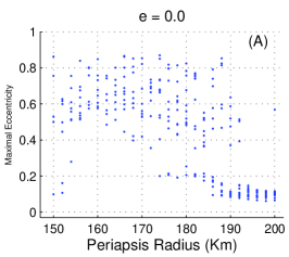
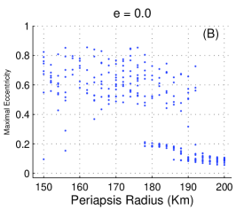
Figure 7: The maximal eccentricity of initially circular orbits about (21) Lutetia after 45 days, considering the one- (A), three- (B) and four-layer structure (C).

Despite similarities among different panels of Fig. 7 and 8, a simple comparison of the tree panels (a,b,c) for each initial eccentricity shows that different internal structures of the asteroid could stabilize or destabilize some orbits. For initially eccentric orbits, (8) shows an increase in the stability region when the initial eccentricity increases. Most important, for all the eccentricities here considered, the stability region increases when the three- and four-layers structures are considered.

Finally, in order to show the effects of the suggested core-mantle structure of (21) Lutetia on the orbital stability, three examples of 3D equatorial orbits after 45 days, are displayed in Figs. 9, 10 and 11. The core-mantle structure can cause orbits to precess or regress around the asteroid, depending on the initial conditions. In the first examples (Fig. 9), considering the uniform structure destabilize the orbit, while the orbit is destabilized considering three-layer structure in the second example. Finally, the four-layer structure stabilizes the orbit of the Fig. 11

6 Conclusion

The computations carried out in this paper were performed based on the suggestion that the asteroid (21) Lutetia, the European space agency’s Rosetta mission target, may have an in-homogeneous density. This lead to the problem of modeling its gravity field considering three different kinds of internal structures (uniform, three-layers and four-layers). Our different models of Lutetia structure were obtained within the Mascon gravity framework, using the shaped polyhedral source, and dividing each tetrahedron into eight equal layers. The shape of Lutetia is presented, viewed from various perspectives after aligning the asteroid with the principal axes of inertia. The harmonic coefficients $C_{n,m}$ and $S_{n,m}$ up to degree 4, considering an uniform bulk density, were computed with respect to the reference radius. Then, two different internal structures for (21) Lutetia were considered to study the orbital dynamics in its vicinity and to examine the effect of the in-homogeneity. Both three-layer and four-layer Lutetia models provided important effects on the external potential. In their study of the gravity field of Vesta, Park et al. (2014) have shown that the thin crust model is the more appropriate representation of Vesta’s internal structure. In our case, the two layer models provide a satisfactory estimation of the gravitational potential, within 150-200 km from the asteroid center of mass, with a maximum relative difference from the uniform density equal to $9.38\times 10^{-4}$. In terms of CPU time requirements, both of the models are somewhat comparable. However, a better close approach of a spacecraft is necessary to fit the real gravity data to found the plausible internal structure of this asteroid.

Correcting the analytical form of the second derivatives of the potential presented in (Chanut, Aljbaae, & Carruba, 2015a), we tested the stability of the equilibria points. We showed that the location of the equilibrium points can be slightly changed by up to 0.351 km. Moreover, the limiting planar figure of the stability against impact gets closer to the body considering the four-layers structure. Finally, in order to examine the potential effects of the in-homogeneity of Lutetia, stability analyses were investigated by testing orbits in an appropriate grid of initial conditions. Generally speaking , the stability region increases when considering the three- and four-layers structure. Future applications of this model could involve the study of the stability of polar orbits, that are more suitable for mapping and reconnaissance purposes.

References

- Barucci et al. (1987) Barucci M. A., Capria M. T., Coradini A., Fulchignoni M., 1987, Icar, 72, 304.
- Barucci et al. (2005) Barucci M. A., et al., 2005, A&A, 430, 313.
- Birlan et al. (2004) Birlan M., Barucci M. A., Vernazza P., Fulchignoni M., Binzel R. P., Bus S. J., Belskaya I., Fornasier S., 2004, NewA, 9, 343.
- Bus & Binzel (2002) Bus S. J., Binzel R. P., 2002, Icar, 158, 146.
- Busarev et al. (2004) Busarev V. V., Bochkov V. V., Prokof’eva V. V., Taran M. N., in The new Rosetta targets, 2004, ASSL, 311, 79–83.
- Carry et al. (2010) Carry B., et al., 2010, A&A, 523, A94.
- Chanut, Aljbaae, & Carruba (2015a) Chanut T. G. G., Aljbaae S., Carruba V., 2015 (a), MNRAS, 450, 374.
- Chanut et al. (2015b) Chanut T. G. G., Winter O. C., Amarante A., Araújo N. C. S., 2015 (b), MNRAS, 452, 1316.
- Chanut, Winter, & Tsuchida (2014) Chanut T. G. G., Winter O. C., Tsuchida M., 2014, MNRAS, 438, 2672
- Coradini et al. (2011) Coradini A., Capaccioni F., Erard S., et al., 2011, Science 334, 492
- DeMeo et al. (2009) DeMeo F. E., Binzel R. P., Slivan S. M., Bus S. J., 2009, Icar, 202, 160
- Descamps et al. (2011) Descamps P., et al., 2011, Icar, 211, 1022
- Dobrovolskis (1996) Dobrovolskis A. R., 1996, Icar, 124, 698
- Gaskell et al. (2008) Gaskell R. W., et al., 2008, M&PS, 43, 1049.
- Giancotti et al. (2014) Giancotti M., Campagnola S., Tsuda Y., Kawaguchi J., 2014, CeMDA, 120, 269.
- Hu & Scheeres (2008) Hu W.-D., Scheeres D. J., 2008, ChJAA, 8, 108.
- Hu & Scheeres (2004) Hu W., Scheeres D. J., 2004, P&SS, 52, 685.
- Hu (2002) Hu W., 2002, Ph.D. Dissertation, University of Michigan.
- Jiang et al. (2014) Jiang Y., Baoyin H., Li J., Li H., 2014, Ap&SS, 349, 83.
- Kaasalainen (2011) Kaasalainen M, 2011, Inverse Problem and Imaging 5, 37-57.
- Konopliv et al. (2014) Konopliv A. S., et al., 2014, Icar, 240, 103.
- Konopliv et al. (2011) Konopliv A. S., Asmar S. W., Bills B. G., Mastrodemos N., Park R. S., Raymond C. A., Smith D. E., Zuber M. T., 2011, SSRv, 163, 461
- Lazzarin et al. (2004) Lazzarin, M., Marchi, S., Magrin, S., Barbieri, C. 2004. Visible spectral properties of asteroid 21 Lutetia, target of Rosetta Mission. Astronomy and Astrophysics 425, L25-L28.
- Lazzarin et al. (2009) Lazzarin M., Marchi S., Moroz L. V., Magrin S., 2009, A&A, 498, 307
- Magrin et al. (2012) Magrin S., et al., 2012, P&SS, 66, 43
- Mirtich (1996) Mirtich B., 1996, Journal of graphics tools, 1, 2.
- Murray & Dermott (1999) Murray C. D., Dermott S. F., 1999, ssd..book.
- Neumann, Breuer, & Spohn (2013) Neumann W., Breuer D., Spohn T., 2013, Icar, 224, 126.
- Park et al. (2014) Park R. S., et al., 2014, Icar, 240, 118.
- Pätzold et al. (2011) Pätzold M., et al., 2011, Sci, 334, 491.
- Rossi, Marzari, & Farinella (1999) Rossi A., Marzari F., Farinella P., 1999, EP&S, 51, 1173
- Scheeres (2012) Scheeres D. J, 2012, JGCD, 35, 987.
- Scheeres & Marzari (2002) Scheeres, D. J.,& Marzari, F., 2002, Journal of the Astronautical Sciences, 50(1), 35
- Scheeres, Williams, & Miller (2000) Scheeres D. J., Williams B. G., Miller J. K., 2000, JGCD, 23, 466
- Scheeres (1999) D. J., Scheeres, 1999, Journal of the Astronautical Sciences, Vol. 47, No. 1, pp. 25-46.
- Scheeres et al. (1998a) Scheeres D. J., Marzari F., Tomasella L., Vanzani V., 1998 (a), P&SS, 46, 649.
- Scheeres et al. (1998b) Scheeres D. J., Ostro S. J., Hudson R. S., DeJong E. M., Suzuki S., 1998 (b), Icar, 132, 53
- Scheeres et al. (1996) Scheeres D. J., Ostro S. J., Hudson R. S., Werner R. A., 1996, Icar, 121, 67.
- Scheeres (1994) Scheeres D. J., 1994, Icar, 110, 225.
- Schulz et al. (2010) Schulz R., Accomazzo A., Küppers M., Schwehm G., Wirth K., 2010, epsc.conf, 18.
- Sierks et al. (2011) Sierks H., et al., 2011, Sci, 334, 487.
- Szebehely (1967) Szebehely V., 1967, torp.book.
- Tholen (1989) Tholen, D., 1989, in Asteroids II (Univ. of Arizona Press), 1139.
- Tricarico & Sykes (2010) Tricarico P., Sykes M. V., 2010, P&SS, 58, 1516
- Tsoulis & Petrović (2001) Tsoulis D., Petrović S., 2001, Geop, 66, 535.
- Wang, Jiang, & Gong (2014) Wang X., Jiang Y., Gong S., 2014, Ap&SS, 353, 105
- Weiss et al. (2012) Weiss B. P., et al., 2012, P&SS, 66, 137
- Werner (1997) Werner R. A., 1997, CG, 23, 1071.
- Werner & Scheeres (1997) Werner R. A., Scheeres D. J., 1997, CeMDA, 65, 313.
- Zuber et al. (2011) Zuber M. T., McSween H. Y., Binzel R. P., Elkins-Tanton L. T., Konopliv A. S., Pieters C. M., Smith D. E., 2011, SSRv, 163, 77.
- Yu & Baoyin (2012) Yu Y., Baoyin H., 2012, AJ, 143, 62.