Non-fundamental Home Bias in International Equity Markets

Abstract

This study investigates the relationship of the equity home bias with 1) the country-level behavioral unfamiliarity, and 2) the home-foreign return correlation. We set the hypotheses that 1) unfamiliarity about foreign equities plays a role in the portfolio set up and 2) the correlation of return on home and foreign equities affects the equity home bias when there is a lack of information about foreign equities. For the empirical analysis, the proportion of respondents to the question “How much do you trust? - People you meet for the first time” is used as a proxy measure for country-specific unfamiliarity. Based on the eleven developed countries for which such data are available, we implement a feasible generalized linear squares (FGLS) method. Empirical results suggest that country-specific unfamiliarity has a significant and positive correlation with the equity home bias. When it comes to the correlation of return between home and foreign equities, we identify that there is a negative correlation with the equity home bias, which is against our hypothesis. Moreover, an excess return on home equities compared to foreign ones is found to have a positive correlation with the equity home bias, which is consistent with the comparative statics only if foreign investors have a sufficiently higher risk aversion than domestic investors. We check the robustness of our empirical analysis by fitting alternative specifications and use a log-transformed measure of the equity home bias, resulting in consistent results with ones with the original measure.

F3, F6, G1, G4

1 Introduction

This paper investigates the role of behavioral bias in international equity markets with information frictions. Investors set an optimal portfolio that offers the highest return, which is equivalent to the highest future wealth. When investors have comprehensive information about foreign equities, they consider a combination of sensible economic factors: returns, transaction costs, risks, and market correlations. In this case, the equity home bias is an outcome of transaction costs, such as differences in regulations and operating costs of local offices for financial institutions. Nevertheless, in reality, investors indeed do not have comprehensive information about foreign financial assets. In this case, a behavioral bias such as unfamiliarity can work as part of the noise on the home country’s information about returns on foreign equities. For example, under a lack of information about foreign equities, home investors may undervalue foreign equities, though they reflect measurable transaction costs. In this study, we investigate whether non-fundamental familiarity about foreign equities is a significant determinant of the equity home bias.

French and Poterba (1991) first pointed out the equity home bias by observing that domestic equities comprise over 90% of equity wealth in the U.S and Japan. Since the 1990s, the equity home bias has been a widely explored puzzle in international financial markets. Lewis (1999) and van Wincoop and Warnock (2010) approach this puzzle with hedge mechanisms. Cooper et al. (2013) suggest that domestic investors expect lower returns on foreign assets due to international transaction costs. Current research analyzes the equity home bias considering both institutional and behavioral frameworks (Lewis (1999) and Cooper et al. (2013)).

Furthermore, despite the high integration of the current international finance market, equity home biases have been relatively stable over time. It is agreed that integration in the international financial market leads to a drastic reduction of the transaction costs incurred from different languages and legal systems. For example, Werner and Tesar (1997) and Coeurdacier and Rey (2013) point out that this bias has been reduced since the onset of financial market integration. However, as Figure 1 shows, the share of domestic equity in the United States and Japan is still over 70%, and its trend is relatively stable, although the global shares of total equity value in each country are less than 60%: ranging from 38% to 54% in the U.S. and from 2% to 3% in Japan between 2001 and 2014. .

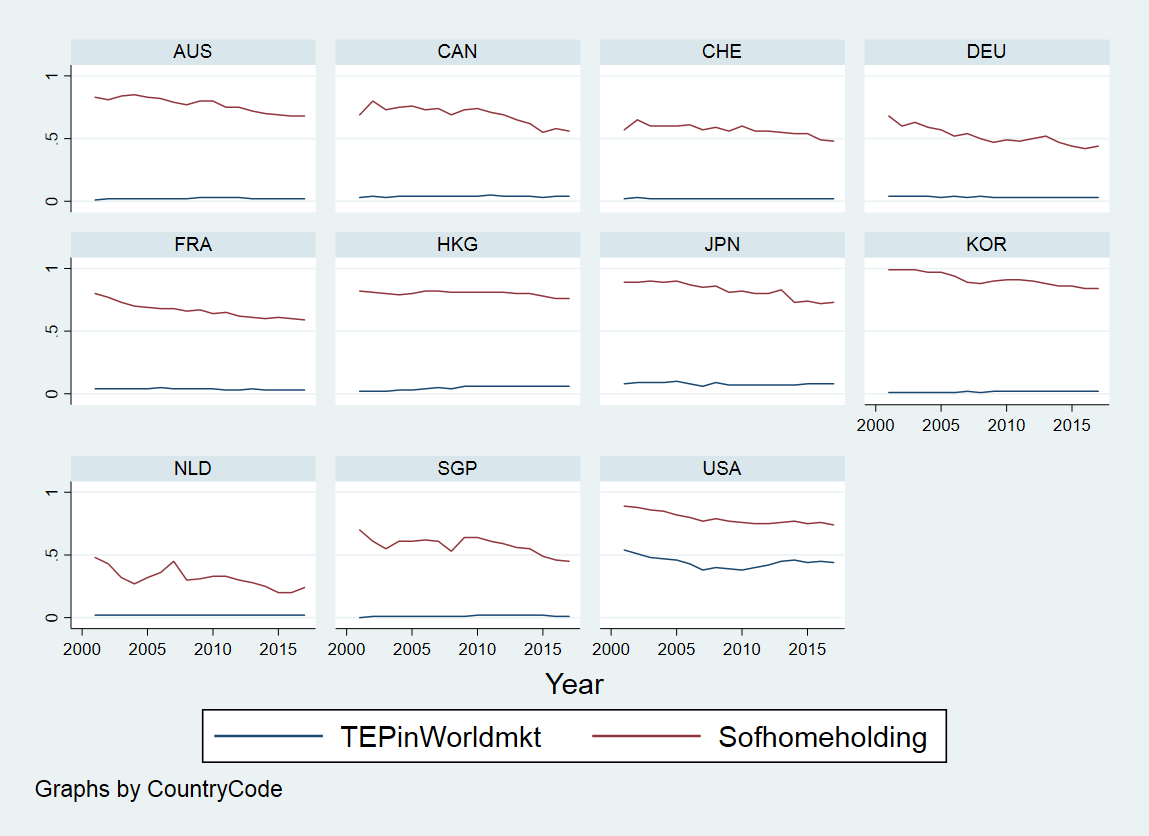
Figure 1: Share of Total Equity Portfolio in World Market Capitalization (Blue) and Share of Holdings of Domestic Equity in Total Equity Portfolio (Red)

• Computed from IMF CPIS and World Bank data

This study focuses on how two factors - namely, 1) information frictions about foreign equities and 2) the correlation between domestic and foreign return on equities - are related to the equity home bias. Moreover, this work empirically shows that non-fundamental unfamiliarity is a significant determinant of the equity home bias. Based on a two-country model modified from that of Chan, Covrig, and Ng (2005) and Foad (2011), the optimal equity shares of both domestic and foreign equity are derived when we employ information frictions on foreign equities. At the optimal share of the portfolio, this study examines how the equity home bias depends on 1) the information frictions on foreign equities and 2) the correlation between domestic and foreign equity returns. For the empirical analysis, we assume that there are information frictions about the foreign equities, and implement a feasible generalized linear squares (FGLS) method. In the empirical analysis, the country-level equity home bias is computed using data from the World Bank and Coordinated Portfolio Invest Survey (CPIS). The country-level proportion of respondents to the survey question, “How much you trust: People you meet for the first time?”, in the World Value Survey (WVS) is exploited as a measure for the level of non-fundamental unfamiliarity, which is an essential factor for noise from the information frictions on foreign equities. In the last part of this research, we conduct additional empirical analyses using transformed measures of the equity home bias.

This work is innovative in two senses. Firstly, we use a novel measure of personal behavior based on publicly available data. The question adopted from the WVS data closely represents the country-level unfamiliarity. Using this data, we support the relationship between country-specific unfamiliarity and the equity home bias when home investors have limited information about foreign equities. Previous studies, such as Huberman (2000), Beugelsdijk and Frijns (2010), and Chan, Covrig, and Ng (2005), investigate the relationship between familiarity and the equity home bias using proxies, such as languages and distance. Secondly, we investigate behavioral factors and market correlation simultaneously.

Comparative statics hypothesize an increase in the equity home bias under the information frictions. Moreover, a positive correlation between domestic and foreign equities leads to a higher equity home bias, which explains that investors have less incentives to buy foreign assets due to higher substitution. In the empirical analysis, assuming that domestic financial markets have information frictions about foreign equities, we verify that unfamiliarity has a significant and positive correlation with the equity home bias. Regarding the correlation of return between home and foreign equities, we find a negative correlation with the equity home bias, which is opposite to the result from the comparative statics. Additionally, an excess return on home equities compared to foreign ones is found to have a positive association with the equity home bias, which is consistent with the comparative statics when foreign investors have a higher risk aversion than domestic investors. To check the robustness of our empirical analysis, we fit alternative estimation models, and use a log-transformed measure of the equity home bias, which turns in consistent results with ones with the original measure.

This paper proceeds as follows. In section 2, related studies are reviewed. Then, we set the theoretical model and provide analytic solutions in section 3. After the theoretical work, in section 4, the hypotheses are tested and the empirical results discussed. Finally, in section 5, the concluding remarks are provided.

2 Related Literature

Traditional studies approach the equity home bias with a transaction cost, such as relevant fees incurred from cross-border financial transactions (Stulz (1981) and Obstfeld and Rogoff (2000)). Beyond transaction costs, there have been numerous studies exploring the determinants of the equity home bias. The ability to hedge domestic or exchange rate risks is considered as one of the most significant determinants of the equity home bias (Cooper and Kaplanis (1986), Cooper and Kaplanis (1994), Mishra (2011), Beck and Fidora (2008) and Coeurdacier and Rey (2013) ). Moreover, asymmetric information (Kang et al. (1997), Ivković and Weisbenner (2005), Foad (2011)) and corporate governance structures (Gelos and Wei (2005)) are suggested as factors associated with the equity home bias.

The equity home bias is also explained as a result of the interaction between financial markets. Quinn and Voth (2008) and Levy and Levy (2014) argue that if markets’ returns move in the same direction, then investors have less incentives to use foreign equities for investment diversification. Comovement of both domestic and foreign returns implies that there is a high substitute relationship between domestic and foreign equities. In this case, foreign equities are not attractive to hedge domestic equity risk. Levy and Levy (2014) show that home bias is proportional to the average correlation between markets, and the proportion is less than 1 .

Recently, there has been a consensus that the equity home bias is an outcome of the combination of behavioral and institutional factors. Using panel data from 38 countries between 2001 and 2010, Bose, MacDonald, and Tsoukas (2015) show that improving financial literacy has a significant impact on reducing the equity home bias, and its impact is amplified in the less financially developed economies. Beugelsdijk and Frijns (2010) suggest that risk aversion and cultural differences relate to unfamiliarity with foreign assets. Huberman (2000) argues that investors overestimate the risk of foreign assets because the foreign assets are less familiar to domestic investors. Most of the familiarity in those works is measured by official languages, the distance between countries or cultural similarities (Grinblatt and Keloharju (2001), Chan, Covrig, and Ng (2005) and Berkel (2007)). Morse and Shive (2011) introduce patriotism. Using the World Values Survey (WVS) data, they show that patriotism can explain marginally five percent of the equity home bias. Barberis and Thaler (2003) introduce belief perseverance, which is the investors’ reluctance to look for evidence that refutes the beliefs.

This study is in line with previous studies, which suggest that the equity home bias arises from a combination of socio-behavioral features, asymmetric information, and financial markets’ interactions. This work is in the context of the results from Huberman (2000), Foad (2010), and Foad (2011) in the sense that investors tend to avoid foreign equities because unfamiliarity plays a role when there is a lack of information about foreign equities. Since this work considers the comovement of domestic-foreign market returns, it is also related to the study by Levy and Levy (2014).

Compared to the previous literature, this work has two distinguishable points. Firstly, it utilizes a novel measure of personal behavior, unfamiliarity, from publicly available data. Secondly, it analyzes both the behavioral factor and market correlation simultaneously.

3 Theoretical Framework

Lewis (1999) and Foad (2011) suggest a mean-variance framework to analyze the equity home bias under information frictions on foreign financial markets. While sharing the spirit of the international capital asset pricing model (ICAPM) of Foad (2011), this work sets the model without inflation and exchange rate. For simplicity, we introduce a mean-variance framework instead of a constant relative risk aversion model (CRRA). Furthermore, to concentrate on the role of unfamiliarity in information frictions about foreign equities, this work does not consider cross-border labor movements such as immigration, which are incorporated in Foad (2011).

Following Ljungqvist and Sargent (2018), we can derive a mean-variance utility from an exponential utility function and a normally distributed return on a portfolio .

In Appendix A, we show how maximizing the expected utility function is equivalent to maximizing the mean-variance utility, which is a linear function of mean and variance of return on a portfolio. Combining the information set, $I_{h}$ for home country and $I_{f}$ for foreign country, and the home investor’s share of both domestic and foreign equity, $w_{h}^{h}$ and $w_{h}^{f}=1-w_{h}^{h}$, we can define the home investor’s portfolio expected return and variance as:

$$E\left(R_{h}^{P}|\,I_{h}\right)=w_{h}^{h}\left[E\left(R^{h}\,|\,I_{h}\right)-c_{h}^{h}\right]+\left(1-w_{h}^{h}\right)\left[E\left(R^{f}\,|\,I_{h}\right)-c_{h}^{f}\right]$$ (1)

$$(\sigma_{h}^{P})^{2}|\,I_{h}=\left(w_{h}^{h}\right)^{2}var\left(R^{h}\,|\,I_{h}\right)+\left(1-w_{h}^{h}\right)^{2}var\left(R^{f}\,|\,I_{h}\right)+$$

$$2\left(w_{h}^{h}\right)\left(1-w_{h}^{h}\right)cov\left(R^{h},\,R^{f}\,|\,I_{h}\right).$$

When it is assumed that short leverage is not allowed, $w_{h}^{h}$ is the non-negative domestic portfolio share of home country’s total investment, while $w_{h}^{f}$ is the foreign portfolio share of domestic portfolio . Also, $R^{h}$ and $R^{f}$ are the expected return of each domestic and foreign equity. $c_{h}^{h}\;\left(c_{h}^{f}\right)$ is defined as the cost of home investors holding domestic (foreign) equity. The objective function of the home investor in mean-variance form is:

$$Max_{w_{h}^{h}}\;w_{h}^{h}\left[E\left(R^{h}\,|\,I_{h}\right)-c_{h}^{h}\right]+\left(1-w_{h}^{h}\right)\left[E\left(R^{f}\,|\,I_{h}\right)-c_{h}^{f}\right]$$ (2)

$$-\dfrac{\lambda_{h}}{2}\left[(\sigma_{h}^{P})^{2}|\,I_{h}\right]$$

where $\lambda_{h}\;(\lambda_{f})$ is home (foreign) investor’s degree of risk aversion. In order to focus on the issue of our interest, we do not incorporate currency differences which are associated with exchange rate risk. Since the mean-variance utility is equivalent to the expected utility of an investor’s future wealth from the portfolio, we can define consumption of a representative investor as the expected future wealth of the portfolio in this framework. Given a positive optimal portfolio share, it implies a positive relationship between domestic equity return and consumption.

From the home investors’ perspective, there are information frictions on foreign equities. Likewise, foreign investors do not have complete information on home equities. Especially, according to Foad (2011), given the information set of $I_{h}$, home investors consider a degree of uncertainty on foreign equities quantified by $\eta_{f}$. Also, foreign investors with $I_{f}$ face risk about home equities in the amount $\eta_{h}$. Denoting $\eta_{h}\;\left(\eta_{f}\right)$ as a variance of return on home (foreign) equity from the perspective of foreign (home) investors with information set $I_{f}\;(I_{h})$, we can describe the following relationships when we assume $u_{f}$ $(u_{h})$ does not have a correlation with $R^{h}\,|\,I_{f}$ $(R^{f}\,|\,I_{h})$:

$$R^{h}\,|\,I_{f}=R^{h}\,|\,I_{h}+u_{f}\;where\;u_{f}\sim\left(0,\,\eta_{f}\right)$$

$$E\left[R^{h}\,|\,I_{f}\right]=E\left[R^{h}\,|\,I_{h}\right]\equiv\mu^{h}$$

$$var\left(R^{h}\,|\,I_{f}\right)=var\left(R^{h}\,|\,I_{h}\right)+\eta_{f}\equiv\left(\sigma^{h}\right)^{2}+\eta_{f}$$

$$R^{f}\,|\,I_{h}=R^{f}\,|\,I_{f}+u_{h}\;where\;u_{h}\sim\left(0,\,\eta_{h}\right)$$

$$E\left[R^{f}\,|\,I_{h}\right]=E\left[R^{f}\,|\,I_{f}\right]\equiv\mu^{f}$$

$$var\left(R^{f}\,|\,I_{h}\right)=var\left(R^{f}\,|\,I_{f}\right)+\eta_{h}\equiv\left(\sigma^{f}\right)^{2}+\eta_{h}$$

where $\left(\sigma^{h}\right)^{2}$ and $\left(\sigma^{f}\right)^{2}$ are the true variances of domestic and foreign assets, respectively. Both home and foreign investors share the expected rate of return of the home (foreign) equity, $\mu^{h}$ and $\mu^{f}$, despite the different information sets. Nevertheless, as foreign investors make more precise predictions regarding the rate of return on foreign equities, the home investors face an additional noise about the foreign equities, with the amount of $\eta_{h}$, beyond the actual variance of foreign equity. Likewise, home investors who are familiar with domestic equities can anticipate the expected return on domestic equities, so foreign investors face an additional noise with the amount of $\eta_{f}$ beyond the real variance of home equity.

For convenience, we assume that the covariance of domestic-foreign equity return is constant and independent of information sets, i.e. $cov\left(R^{h},\,R^{f}\,|\,I_{h}\right)=cov\left(R^{h},\,R^{f}\,|\,I_{f}\right)=\sigma^{hf}$.

From Equation (2), assuming an interior solution, the optimal share of domestic and foreign equities for home investors, $w_{h}^{h}$ and $w_{h}^{f}$, are

$$w_{h}^{h}=\dfrac{1}{\lambda_{h}}\dfrac{\left(\mu^{h}-c_{h}^{h}\right)-\left(\mu^{f}-c_{h}^{f}\right)}{\left(\sigma^{h}\right)^{2}+\left(\sigma^{f}\right)^{2}-2\sigma^{hf}+\eta_{h}}+\dfrac{\left(\sigma^{f}\right)^{2}-\sigma^{hf}+\eta_{h}}{\left(\sigma^{h}\right)^{2}+\left(\sigma^{f}\right)^{2}-2\sigma^{hf}+\eta_{h}}$$ (3)

$$w_{h}^{f}=\dfrac{1}{\lambda_{h}}\dfrac{\left(\mu^{f}-c_{h}^{f}\right)-\left(\mu^{h}-c_{h}^{h}\right)}{\left(\sigma^{h}\right)^{2}+\left(\sigma^{f}\right)^{2}-2\sigma^{hf}+\eta_{h}}+\dfrac{\left(\sigma^{h}\right)^{2}-\sigma^{hf}}{\left(\sigma^{h}\right)^{2}+\left(\sigma^{f}\right)^{2}-2\sigma^{hf}+\eta_{h}}.$$

The market-clearing condition is required for equilibrium in the international financial markets. Let us denote the proportion of global total equity portfolio owned by a home (foreign) country as $\Pi_{h}\;\left(\Pi_{f}\right)$. That is, $\Pi_{h}$ and $\Pi_{f}$, can be interpreted as the share of world wealth belonging to home and foreign countries. The market clearing condition is,

$$\Pi_{h}w_{h}^{h}+\underbrace{\left(1-\Pi_{h}\right)}_{\equiv\Pi_{f}}w_{f}^{h}=w^{h*}=\\ \Pi_{h}\dfrac{1}{\lambda_{h}}\dfrac{\left(\mu^{h}-c_{h}^{h}\right)-\left(\mu^{f}-c_{h}^{f}\right)}{\left(\sigma^{h}\right)^{2}+\left(\sigma^{f}\right)^{2}-2\sigma^{hf}+\eta_{h}}+\Pi_{h}\dfrac{\left(\sigma^{f}\right)^{2}-\sigma^{hf}+\eta_{h}}{\left(\sigma^{h}\right)^{2}+\left(\sigma^{f}\right)^{2}-2\sigma^{hf}+\eta_{h}}\\ +\left(1-\Pi_{h}\right)\dfrac{1}{\lambda_{f}}\dfrac{\left(\mu^{h}-c_{f}^{h}\right)-\left(\mu^{f}-c_{f}^{f}\right)}{\left(\sigma^{h}\right)^{2}+\left(\sigma^{f}\right)^{2}-2\sigma^{hf}+\eta_{f}}+\left(1-\Pi_{h}\right)\dfrac{\left(\sigma^{f}\right)^{2}-\sigma^{hf}}{\left(\sigma^{h}\right)^{2}+\left(\sigma^{f}\right)^{2}-2\sigma^{hf}+\eta_{f}}$$ (4)

$$\Pi_{h}w_{h}^{f}+\underbrace{\left(1-\Pi_{h}\right)}_{\equiv\Pi_{f}}w_{f}^{f}=w^{f*}=\\ \Pi_{h}\dfrac{1}{\lambda_{h}}\dfrac{\left(\mu^{f}-c_{h}^{f}\right)-\left(\mu^{h}-c_{h}^{h}\right)}{\left(\sigma^{h}\right)^{2}+\left(\sigma^{f}\right)^{2}-2\sigma^{hf}+\eta_{h}}+\Pi_{h}\dfrac{\left(\sigma^{h}\right)^{2}-\sigma^{hf}}{\left(\sigma^{h}\right)^{2}+\left(\sigma^{f}\right)^{2}-2\sigma^{hf}+\eta_{h}}\\ +\left(1-\Pi_{h}\right)\dfrac{1}{\lambda_{f}}\dfrac{\left(\mu^{f}-c_{f}^{f}\right)-\left(\mu^{h}-c_{f}^{h}\right)}{\left(\sigma^{h}\right)^{2}+\left(\sigma^{f}\right)^{2}-2\sigma^{hf}+\eta_{f}}+\left(1-\Pi_{h}\right)\dfrac{\left(\sigma^{h}\right)^{2}-\sigma^{hf}+\eta_{f}}{\left(\sigma^{h}\right)^{2}+\left(\sigma^{f}\right)^{2}-2\sigma^{hf}+\eta_{f}}$$

where $w^{h*}\;\left(w^{f*}\right)$ is the home’s (foreign’s) domestic market capitalization share in the international financial market. By combining Equations (3) and (4), one can derive the equity home bias from the perspective of a home country, $(w_{h}^{h}-w^{h*})$:

$$w_{h}^{h}-w^{h*}=\\ \left(1-\Pi_{h}\right)\dfrac{1}{\lambda_{h}}\dfrac{\left(\mu^{h}-c_{h}^{h}\right)-\left(\mu^{f}-c_{h}^{f}\right)}{\left(\sigma^{h}\right)^{2}+\left(\sigma^{f}\right)^{2}-2\sigma^{hf}+\eta_{h}}+\left(1-\Pi_{h}\right)\dfrac{\left(\sigma^{f}\right)^{2}-\sigma^{hf}+\eta_{h}}{\left(\sigma^{h}\right)^{2}+\left(\sigma^{f}\right)^{2}-2\sigma^{hf}+\eta_{h}}\\ -\left(1-\Pi_{h}\right)\dfrac{1}{\lambda_{f}}\dfrac{\left(\mu^{h}-c_{f}^{h}\right)-\left(\mu^{f}-c_{f}^{f}\right)}{\left(\sigma^{h}\right)^{2}+\left(\sigma^{f}\right)^{2}-2\sigma^{hf}+\eta_{f}}-\left(1-\Pi_{h}\right)\dfrac{\left(\sigma^{f}\right)^{2}-\sigma^{hf}}{\left(\sigma^{h}\right)^{2}+\left(\sigma^{f}\right)^{2}-2\sigma^{hf}+\eta_{f}}\;.$$ (5)

Based on the property of the variance of two returns, we can easily verify that $Var(R^{h}-R^{f})=\left(\sigma^{h}\right)^{2}+\left(\sigma^{f}\right)^{2}-2\sigma^{hf}$ is positive. The first two terms of $\left(w_{h}^{h}-w^{h*}\right)$ in Equation (5) are related to domestic investors. The first term explains the relationship between the relative net return on home equity and the equity home bias. It is sensible that home investors tend to increase their share of home equities if the net return on domestic equities is relatively high compared to the one on foreign equities. The second term shows the relationship between the volatility of foreign equity and the equity home bias, given the information frictions of the home country. The latter two terms are associated with foreign investors’ behavior. Foreign investors increase the share of home equities if home equities give a relatively high net return compared to foreign equities (the third term). Also, foreign investors tend to avoid the volatility of foreign equities by purchasing home equities (the fourth term) .

Moreover, assuming symmetric uncertainty, i.e. $\eta_{h}=\eta_{f}$, and transaction cost, i.e. $c_{h}^{h}=c_{h}^{f}$ and $c_{f}^{h}=c_{f}^{f}$, we expect that the equity home bias depends on the correlation between investors’ consumption and return on domestic equities only when the degree of risk aversion $(\lambda)$ is heterogeneous across countries. Based on the current framework, consumption is defined as future wealth from investment. Therefore, we can identify that the correlation between consumption and domestic return is non-negative, as the optimal shares of both home and foreign equities are between zero and one. For example, if there is a higher net return on the domestic equity compared to the foreign equities, $(\mu^{h}>\mu^{f})$, the equity home bias is increasing in return on domestic equity only when foreign investors have a higher degree of risk aversion than domestic investors $(\lambda_{f}>\lambda_{h})$. This implies that domestic investors face a higher correlation between consumption and domestic equity return compared to foreign investors. In such a case, domestic investors tend to increase the domestic equity share when the domestic equities give a relatively higher return. Alternatively, if domestic investors are relatively less sensitive to the portfolio return than foreign investors $(\lambda_{f}<\lambda_{h})$, the equity home bias is decreasing in return on domestic equities because foreign investors would increase their domestic equity share more than domestic investors when a domestic return is higher. When both domestic and foreign investors have symmetric sensitivity of their consumption to the return on the portfolio $(\lambda_{f}=\lambda_{h})$, the equity home bias is independent of the correlation between consumption and domestic equity return, because the same correlation level between consumption and domestic return gives both investors to set the same share of domestic equity.

To simplify the comparative statics, we can additionally assume that investors in both countries have the same levels of degree of risk aversion, i.e., $\lambda_{h}=\lambda_{f}$. Then, the equity home bias described in Equation (5) is simplified without the assumption of an identical net return across countries $(\mu^{h}=\mu^{f})$, such as Equation (6):

$$w_{h}^{h}-w^{h*}=\left(1-\Pi_{h}\right)\left(w_{h}^{h}-w_{h}^{f}\right)=\left(1-\Pi_{h}\right)\dfrac{\eta}{\left(\sigma^{h}\right)^{2}+\left(\sigma^{f}\right)^{2}-2\sigma^{hf}+\eta}.$$ (6)

By taking partial derivatives with respect to either $\eta$ and $\sigma^{hf}$, one can get $\frac{\partial\left(w_{h}^{h}-w^{h*}\right)}{\partial\eta}>0$ and $\frac{\partial\left(w_{h}^{h}-w^{h*}\right)}{\partial\sigma_{hf}}>0$ . Given that $\eta$ is positive, a higher correlation between home and foreign assets leads to a higher equity home bias, which is consistent with the results of Levy and Levy (2014), in which they argue that higher substitution between home and foreign equities leads to a higher home bias because investors do not have incentives to convert their domestic equities to foreign ones. In the case that the home equity is a substitute for the foreign equity, i.e., a positive $\sigma^{hf}$, the existence of information frictions on foreign equity amplifies the equity home bias.

4 Empirical Analysis

4.1 Measures

As there is no specific data about the equity home bias, this study measures the equity home bias following the procedure in Coeurdacier and Rey (2013). We can define the equity home bias in the home country as the difference between (A) the proportion of domestic equity in the total equity portfolio of a home country and (B) the share of a home country’s capitalization in total world equity market capitalization, i.e., (A) - (B). The following equation (7) defines the measure of equity home bias in this study:

$$EHB_{h}=1-\dfrac{\frac{HFE_{h}}{TEP_{h}}}{\frac{DMC_{h}}{World\;Total\;Market\;Cap}}$$ (7)

where $EHB_{h}$ is the equity home bias, $HFE_{h}$ denotes holding of foreign equity by the home country, $TEP_{h}$ is the total equity portfolio in the home country, and $DMC_{h}$ represents domestic market capitalization. Also, in order to get the total equity portfolio in the home country $(TEP_{h})$ in Equation (7), the following relationship should be satisfied:

$$TEP_{h}=DMC_{h}+HFE_{h}-HFE_{f}$$ (8)

where $HFE_{f}$ is the foreign holdings of domestic equity. If the portfolio of the home country is perfectly diversified, $EHB_{h}$ should be zero based on the international capital asset pricing model (ICAPM) (Coeurdacier and Rey (2013)).

For a measure of unfamiliarity under information frictions about foreign equities, this work utilizes the proportion of respondents who answered the survey question, “How much you trust: People you meet for the first time?” from the World Value Survey (WVS) (WVS (2014)). Although Hofstede’s cultural dimensions data set captures several aspects of country-specific differences, this is not precisely consistent with country-specific unfamiliarity about foreign equities. For example, individualism and uncertainty avoidance in Hofstede’s data are not sufficient alternatives to unfamiliarity .

4.2 Data

4.2.1 Equity Home Bias

Equity home bias can be calculated using domestic market capitalization and total portfolio investment across the border with Equations (7) and (8). The World Bank (WB) and the World Federation of Exchanges (WFE) provide domestic market capitalization data in terms of market capitalization in equity. This paper exploits the WB data set because it provides country-level information . Also, total portfolio investment across the border by nations can be extracted from the Coordinated Portfolio Investment Survey (CPIS) of the IMF. In CPIS, there are total portfolio investment assets and liabilities in equity for each country, which are equivalent to domestic holdings of foreign equities and foreign holdings of domestic equities.

The period for the empirical analysis in this study is 17 years, from 2001 to 2017. Data on market capitalization earlier than 2001 are available. In contrast, the data for the cross-border investment in equity in CPIS has been published only since 2001. Data for 2018 are not employed because of missing values for some countries. To construct a balanced panel data set, the sample comprises 11 countries (Australia, Canada, France, Germany, Hong Kong, Japan, South Korea, the Netherlands, Singapore, Switzerland, and the U.S.) that have reported domestic market capitalization to WB and cross-border portfolios to CPIS without missing values among developed countries with the WVS data.

All of the selected countries have equity home bias, as shown in Figure 2. Most of the non-EU countries, for example, Australia, Canada, Hong Kong, Japan, South Korea, and the U.S., show a higher equity home bias compared to the selected EU-countries. For instance, in 2014, the equity home biases in three non-EU countries were 71% (Japan), 57% (U.S.), 53% (Switzerland) and 60% (Canada). Although France has shown temporarily higher home biases than the U.S. and Canada earlier in the 21st century, other selected countries in the EU, for example, Germany and the Netherlands, exhibit significantly lower home equity biases. Capital movement freedom may explain this feature within EU countries .

As shown in Figure 2, the bias of each country was smaller in 2017 compared to 2001, even if there were fluctuations. The simple average of equity home bias in these 11 countries was 74% in 2001, which contrasts with an average home bias of 56% in 2017. Considering those eleven countries are highly developed countries whose financial markets are deeply integrated, the equity home bias puzzle cannot be explained only by the transaction cost, including differences in legal systems and languages.

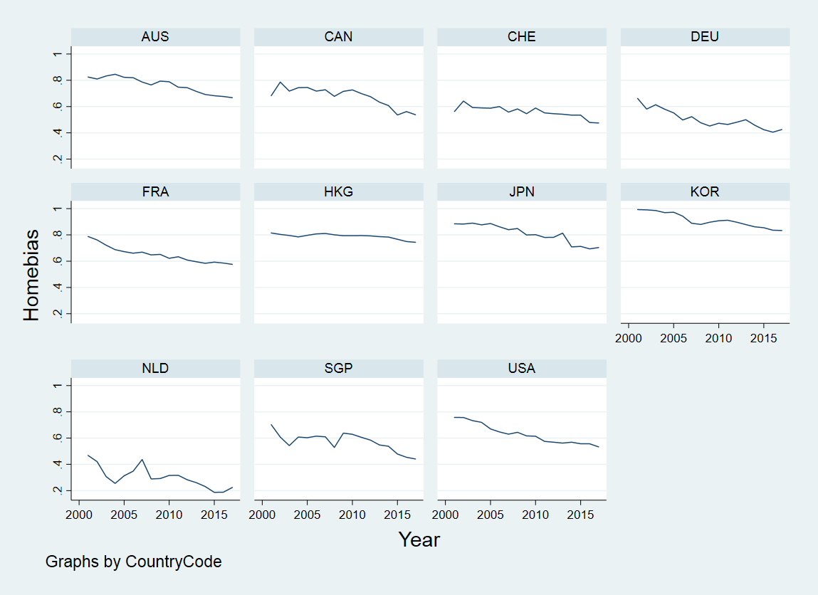
Figure 2: Equity Home Bias in Several Developed Countries

• Computed from IMF CPIS and World Bank data

4.2.2 Non-fundamental unfamiliarity

Non-fundamental unfamiliarity is measured from the WVS dataset, survey data regarding cultural features by nations. WVS has conducted six waves since 1990; it has interviewed between 1,000 and 2,000 people in each nation per wave. Given this dataset, this paper considers the proportion of people who respond “Do not trust much” or “Do not trust at all” to the question: “ I ’d like to ask you how much you trust people from various groups. Could you tell me for each whether you trust people from this group completely, somewhat, not very much or not at all? - People you meet for the first time” in each country .

Figure 3 shows the individual mistrust from unfamiliarity of others by selected nations. Except for Canada and Switzerland, over half of respondents in selected countries stated that they do not trust strangers. Specifically, over 70% of German, Italian and Japanese respondents showed mistrust toward unfamiliar people.

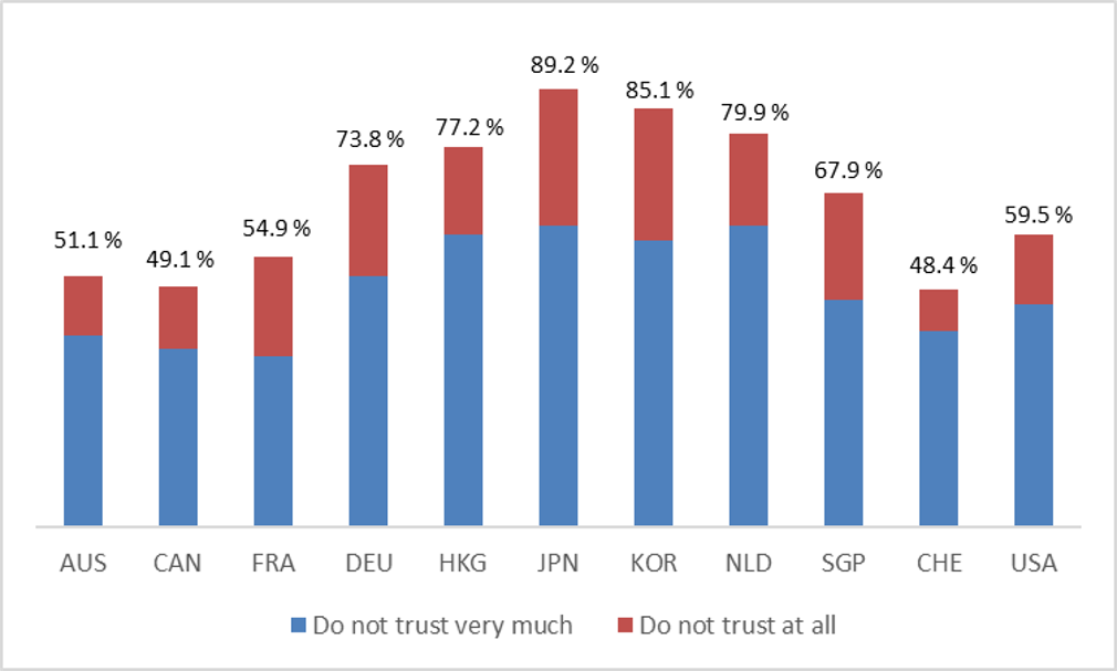
Figure 3: The Portion of Respondents for “Do not trust much” or “Do not trust at all” to the Question: “ I ‘d like to ask you how much you trust people from various groups. Could you tell me for each whether you trust people from this group completely, somewhat, not very much or not at all? - People you meet for the first time.”

• Computed from the WVS data

4.3 Empirical Model and Results

In the empirical analysis, a panel analysis is implemented. As country-specific unfamiliarity is time-invariant in this set up, we conduct a feasible generalized linear squared regression (FGLS) method. Moreover, the FGLS method is useful when the error structure across the panels is heteroskedastic and correlated.

Our variables of interest are 1) country-level unfamiliarity, 2) the correlation of return between domestic and foreign equities, and 3) the difference in annual returns between domestic and foreign equities. Regarding country-level unfamiliarity, we use the portion of respondents for “Do not trust much” or “Do not trust at all” to the WVS question: “Do you trust people you meet for the first time?”

For a measure of the correlation of return between domestic and foreign equities, the rate of return on the Global Dow Jones index is assumed as the return on foreign equity. The benchmark equity index in each nation is treated as the equity of the home country .

Based on the daily rate of return on those indexes, we compute the annual correlation of returns between domestic and foreign equities for sample countries. The difference in annual returns between domestic and foreign equities represents the amount of excess return on the local benchmark index compared to the Global Dow Jones index in each country .

In terms of control variables, we introduce 1) a Euro currency area dummy, and 2) a city-level market dummy, and 3) the GDP growth rate. The Euro currency area dummy stands for free capital movement among the member countries of the currency union in the European Union (EU). Also, we introduce a dummy variable that represents city-level markets, Hong Kong and Singapore. Those financial markets are highly depend on international financial transactions. Table 1 offers summary statistics for the variables used. A country-level summary of statistics is attached in Section C .

Since there is a decreasing trend in equity home bias in each country, we control for the trend in equity home bias by adding year as a control variable. Based on a fixed-effect analysis (FE) by regressing the equity home bias on the year variable, the estimated coefficient for the year variable is -0.11 with a standard error of 0.0005, which is significant at the 1% level.

Table 1: Summary Statistics (Aggregate Level)

Variable	Mean	Std. Dev.	Minimum	Maximum	# of Obs.
Home Bias	0.652	0.173	0.187	0.993	187
Unfamiliarity	0.668	0.144	0.480	0.890	11
Correlation with foreign return	0.582	0.193	0.162	0.869	187
Difference in return between home and foreign equities	-0.012	0.113	-0.312	0.355	187
Hong Kong and Singapore	-	-	0	1	11
GDP growth rate	0.024	0.024	-0.056	0.145	187
Euro currency area	-	-	0	1	11
Year	-	-	2001	2017	17

We construct five estimation models to investigate the relationship of unfamiliarity with the equity home bias. Model 1 is a benchmark model. The equity home bias is treated as the dependent variable. Also, unfamiliarity, GDP growth rate, and the Euro currency area dummy are incorporated as explanatory variables. In model 2, the correlation of returns between home and global equities is included to verify whether a higher substitution between domestic and global equity leads to a higher equity home bias. In model 3, the correlation between local and global equity returns is replaced with the difference in return between domestic and global equities to test whether an excess return on home equities compared to the global equity has a positive relationship with equity home bias. In model 4, both the correlation and the difference with the global returns are considered for the estimation. Finally, in Model 5, we control for the city-level global financial markets, Hong Kong and Singapore.

Table 2: Summary of Empirical Results (Original Equity Home Bias across Sample Countries)

Variables	Model 1	Model 2	Model 3	Model 4	Model 5
Unfamiliarity	0.247***	0.074***	0.239***	0.071***	0.110***
	(0.010)	(0.010)	(0.010)	(0.013)	(0.013)
Correlation with foreign return		-0.305***		-0.302***	-0.313***
		(0.018)		(0.021)	(0.023)
Difference in return b/t			0.090***	0.112***	0.100***
home and foreign equities			(0.010)	(0.013)	(0.014)
Hong Kong and Singapore					-0.100***
					(0.008)
GDP growth rate	-0.036	-0.305***	0.046	-0.211**	0.163
	(0.039)	(0.090)	(0.068)	(0.103)	(0.102)
Euro currency area	-0.238***	-0.149***	-0.235***	-0.137***	-0.154***
	(0.004)	(0.006)	(0.006)	(0.005)	(0.006)
Year	-0.011***	-0.012***	-0.011***	-0.012***	-0.012***
	(0.000)	(0.001)	(0.000)	(0.001)	(0.001)
Constant	22.034***	24.242***	22.599***	24.649***	24.413***
	(0.300)	(1.029)	(0.712)	(1.168)	(1.045)
Wald $\chi^{2}$	37668.14***	3616.48***	9289.05***	1795.88***	2410.58***
(Degree of freedom)	(4)	(5)	(5)	(6)	(7)

• *** $p<0.01$, ** $p<0.05$, and * $p<0.1$

• Estimated coefficients (top) and standard errors (bottom, within parenthesis)

Table 2 reports the results from the empirical analysis. Among the five estimation models, Model 4 is the preferred specification. Model 4 shows the highest degree of goodness-of-fit in terms of the smallest Wald chi-square statistic, as shown in the last row of Table 2. It implies that Model 4 contains significant explanatory variables necessary in the empirical analysis with the least redundancy associated with an insignificant variable. It also suggests that Model 4 is neither under- nor over-specified compared to the other models.

We find a significantly positive relationship of country-level unfamiliarity with the equity home bias. The coefficient estimates from Models 1 and 3 in which the correlation of equity returns between two equities is not included are 0.24. In the case of Models 2 and 4 that incorporate the correlation of returns, the coefficient estimates are 0.07. In model 5 that controls for Hong Kong and Singapore, the coefficient estimate is 0.1. Even though the point estimates are different across the empirical models, they are all positive at a 1% significance level. In sum, the equity home bias is positively related to country-specific unfamiliarity.

As per the correlation between home and foreign equity returns, the results from the empirical analysis show a negative relationship with the equity home bias. The estimates of coefficients are between -0.31 and -0.30 at a 1% significance level across empirical models. Those results contrast with our hypothesis from the comparative statics in Section 3 and the results from Levy and Levy (2014) .

The difference in return between home and foreign equities shows a positive relationship with the equity home bias. The estimated coefficient is between 0.09 and 0.12 at a 1% significance level. Those results are opposite to our expectation under the assumption of symmetric degree of risk aversion $(\lambda_{f}=\lambda_{h})$ and transaction costs of obtaining equities, as shown in Equations (5) and (6) of Section 3. The empirical results suggest that home investors acquire home equities more than foreign investors when there is an excess return on home equities compared to foreign ones. Those results are consistent with the ones from the theoretical framework under the assumption that foreign investors have a higher degree risk aversion than domestic investors $(\lambda_{f}>\lambda_{h})$.

Additionally, we can identify how the equity home bias is associated with other control variables. Firstly, we do not find a consistent result regarding the correlation between the GDP growth rate and the equity home bias. The coefficient is -0.3 ~-0.2 in Models 2 and 4, while we do not find any significant results from Models 1 and 3.

A city dummy that represents the city-level independent financial markets, Hong Kong and Singapore, has a negative relationship with the equity home bias; the estimate of coefficient is -0.1 at a 1% significance level in Model 5. This result is consistent with the fact that both regions have acted as international financial hubs in Asia. Since most of the financial transactions associated with Asian countries depend on international finance in those city-level markets, the equity home bias in those regions is at a lower level compared to Korea and Japan.

Furthermore, freedom of capital movement among Euro currency members (Eurozone) has a negative correlation with the equity home bias. The empirical results show a negative relationship between the Euro currency area dummy and the equity home bias with coefficients ranging between -0.24 and -0.14 depending on the models. In sum, this Euro currency area dummy variable can explain a relatively lower level of home equity bias in the three sample countries whose currency is the Euro (France, Germany, and the Netherlands), and we can interpret those results as a lower equity home bias in the Eurozone because of the free capital movement between member countries.

Regarding a trend of the equity home bias, we determine that the equity home bias has decreased over time. The estimate of coefficient is -0.012 $\sim$ -0.011 at a 1% significance level.

4.4 Empirical Results with A Transformed Measure of Unfamiliarity

As reported in Tables 1 and 5 of the previous subsection, the predicted values of the equity home bias are less than 1, which is consistent with the support of the primary measure of equity home bias defined in Equation (7) , such as $(-\infty,\,1]$.

In this part, we transformed the measure of the equity home bias with a larger support, $(-\infty,\,+\infty)$, and checked whether the empirical results are consistent with ones from the original data set. Specifically, we defined the latter part in the definition of the equity home bias described in Equation (7) as $Q_{h}$, such as:

$$Q_{h}\equiv\dfrac{\frac{HFE_{h}}{TEP_{h}}}{\frac{DMC_{h}}{World\;Total\;Market\;Cap}}$$ (9)

where $Q_{h}$ is the home country’s holding portion of foreign equity normalized by the share of its domestic market capitalization share in the world market. As all the values in Equation (9) are non-negative, $Q_{h}$ should be also non-negative, $(Q_{h}\geq 0)$. Then, we took a log-transformation and defined the measure as $g_{h}$ by converting this transformed value into negative, as in Equation (10):

$$g_{h}\equiv-ln(Q_{h})$$ (10)

where the support of $g_{h}$ is ranging from $-\infty$ to $+\infty$. And, the measure $g_{h}$ is positively associated with the equity home bias.

We maintain the previous five estimation models. Therefore, a benchmark model, Model 1, focuses only on country-level unfamiliarity controlling for GDP growth rate and Euro currency area dummy. We include the correlation of returns between home and global equities in Model 2, while we replace the correlation of equity returns with the difference in return between domestic and global equities in Model 3. In model 4, both correlation and difference of returns between home and global equities are incorporated. Lastly, city-level independent markets are considered in Model 5.

The results from the modified support of the equity home bias are reported in Table 3. It can be observed that the results are consistent with ones in the previous part that utilizes the original measure of the equity home bias defined in Equation (7). Among the five estimation models, Model 5 shows the best fit for the empirical analysis in the log-transformed measure case: The Wald chi-square statistic shows the lowest value, 974.77.

Table 3: Summary of Empirical Results (Transformed Equity Home Bias to the Support between $-\infty$ and $+\infty$, $(-\infty,\,+\infty)$)

Variables	Model 1	Model 2	Model 3	Model 4	Model 5
Unfamiliarity	1.848***	1.292***	1.742***	1.126***	1.292***
	(0.035)	(0.063)	(0.054)	(0.076)	(0.082)
Corr. with foreign return		-1.044***		-1.113***	-1.125***
		(0.064)		(0.084)	(0.100)
Difference in return b/t			0.704***	0.767***	0.624***
home and foreign equities			(0.071)	(0.079)	(0.089)
Hong Kong and Singapore					-0.491***
					(0.062)
GDP growth rate	0.917***	0.119	1.297***	0.189	2.012***
	(0.244)	(0.260)	(0.367)	(0.382)	(0.508)
Euro currency area	-0.773***	-0.464***	-0.732***	-0.401***	-0.479***
	(0.010)	(0.019)	(0.018)	(0.021)	(0.024)
Year	-0.046***	-0.048***	-0.045***	-0.048***	-0.048***
	(0.001)	(0.001)	(0.002)	(0.002)	(0.003)
Constant	92.941***	97.643***	90.537***	97.140***	97.389***
	(2.080)	(2.743)	(4.663)	(4.340)	(5.641)
Wald $\chi^{2}$	18221.04***	3497.20***	2856.06***	1256.26***	974.77***
(Degree of freedom)	(4)	(5)	(5)	(6)	(7)

• *** $p<0.01$, ** $p<0.05$, and * $p<0.1$

• Estimated coefficients (top) and standard errors (bottom, within parenthesis)

• Measure of country-level equity home bias is transformed with the support of $(-\infty,\,+\infty)$

As per the country-level unfamiliarity, we find that it has a positive correlation with the equity home bias. The coefficients of estimates range from 1.29 to 1.87 at a 1% significance level. The estimated coefficients are higher than 1.7 when the empirical model does not incorporate the correlation of returns between two equities. In contrast, the coefficients are smaller when the correlation of equity returns is included in the model.

In terms of other variables of our interest, we also find that the relationships between the equity home bias and other variables of our interest are empirically consistent with the results obtained by the original equity home bias measure. Regarding the correlation between home and foreign equity returns, the negative estimates of coefficients at a 1% significance level offers consistency with ones from the empirical analysis in the previous part; they are still opposed to the hypothesis from the comparative statics. The estimated coefficients are between -1.13 and -1.04 at a 1% significance level across the empirical models. Moreover, the empirical results also show that an excess return on domestic equity positively correlates with the equity home bias. The estimates of coefficients are significantly positive at a 1% level, ranging from 0.62 to 0.76.

Consistent with the empirical results in the previous part, the equity home bias has a negative relationship with the currency union, such as the Euro area, and the modified measure of the equity home bias is also decreasing over time.

5 Conclusion

Equity home bias is relatively stable over time despite a higher international financial market integration. This study incorporates information frictions about the return on foreign equity as a factor causing the equity home bias. We hypothesize that investors depend on country-specific non-fundamental behavioral factors when there are information frictions on foreign equities, which raises the equity home bias. Furthermore, based on the substitutability of equities across countries, we hypothesize that the correlation of return between home and foreign equities positively relates to the equity home bias.

In the first part of this research, we derive comparative statics describing relationships between the equity home bias and either information frictions or the home-foreign return correlation. Assuming an identical degree of 1) risk aversion and of 2) uncertainty about foreign equity return across countries, an analytical relationship is derived stating that the equity home bias is associated with information frictions about return on foreign equities. Comparative statics also hypothesize that the correlation of return between home and foreign equities raises the equity home bias. In the second part, this work assumes that portfolios may depend on the unfamiliarity about foreign equities. In the empirical analysis, we hypothesize that unfamiliarity positively associates with the equity home bias. Also, to account for the effect of substitution of equities across countries, we hypothesize that correlation of return between home and foreign equities raises the equity home bias.

Based on a panel consisting of eleven developed countries, the empirical analysis tests the hypotheses described above. We introduce the proportion of respondents to the question, ”Could you tell me for each whether you trust people from this group completely, somewhat, not very much or not at all? - People you meet for the first time”, as as a proxy for the country-specific unfamiliarity from the WVS. For the measure of return correlation return between home and foreign equities, we use an annual correlation of return between the domestic benchmark index and the Global Dow Jones index. We incorporate 1) the difference in return between the domestic benchmark index and Global Dow Jones index, 2) city-level markets such as Hong Kong and Singapore, 3) GDP growth rate, and 4) Euro currency area to the empirical model. We also include time as a regressor because the equity home bias has a decreasing trend.

Setting up five estimation models, we implement an FGLS method allowing heteroskedasticity and correlation across panels. Model 1 considers only country-level unfamiliarity. Model 2 adds the correlation of return between domestic and foreign equities to Model 1. In contrast, Model 3 replaces this return correlation in Model 2 with the excess return on domestic equity. Model 4 employs all the variables of our interest in Model 4. Model 5 adds a dummy representing the city-level markets in Asia to Model 4.

The results from the empirical analysis show a positive relationship between the country-level unfamiliarity and the equity home bias. The coefficient estimates range from 0.07 to 0.24. In contrast to Levy and Levy (2014), the coefficient estimates for the correlation of return between home and foreign equities are negative at a 1% significance level. Besides, an excess return on home equities compared to foreign ones shows a positive correlation with the equity home bias. This positive correlation is consistent with the comparative statics when foreign investors have a higher risk aversion than domestic investors.

To check the robustness of the empirical analysis, we apply a log-transformed measure of the equity home bias to the five estimation models already defined. The empirical results are consistent with the ones using the original measure. Regarding the country-level unfamiliarity, the coefficient estimates are significantly positive, ranging from 1.1 to 1.8. Counter to the hypothesized theoretical relationships, the correlation of return between domestic and foreign equities shows a negative relationship with the equity home bias; the estimates of coefficients are ranging from -1.1 to -1.0. Moreover, the excess return on domestic equity shows a positive correlation with the equity home bias, which is also opposite to the comparative statics results under the assumption of symmetric degree of risk aversion and transaction costs of purchasing equities.

Both theoretical and empirical results show that country-level unfamiliarity positively relates to the equity home bias. Specifically, in the empirical analysis, the WVS data publicly available is exploited for a measure of unfamiliarity. This work leaves an in-depth exploration with a larger dataset for future research. This work accounts for only countries with a highly integrated equity market. Therefore, most developing markets are not included in the sample of empirical analysis. A dataset with extended time-series is expected to provide additional information about the relationship between the country-specific unfamiliarity and the equity home bias.

Appendix A Getting a Mean-variance Utility from an Expected Utility Function (Ljungqvist and Sargent (2018))

Without loss of generality, a home investor plans to invest his initial wealth $W_{h}$ in domestic and foreign assets. Given $R_{h}^{P}$ as the random rate of aggregate return on the home investor’s portfolio, we can denote the home investor’s future wealth as $\tilde{W}_{h}=W_{h}\left(1+R_{h}^{P}\right)$. Given $W_{h}$, we can simplify the investor’s utility in terms of his future wealth, $U\left(\tilde{W}_{h}\right)$, as $U\left(R_{h}^{P}\right)$ because $\tilde{W}_{h}$ is fully determined by $R_{h}^{P}$. The utility function is described in Equation (11):

$$E\left[U\left(R_{h}^{P}\right)\right]=E\left[-e^{-\lambda_{h}R_{h}^{P}}\right].$$ (11)

where $\lambda_{h}$ is a parameter of exponential utility function. From the property of exponential utility function, we can determine that the parameter in exponential utility function, $\lambda$, is the Arrow-Pratt index of absolute risk aversion because:

$$r.a.=-\frac{U^{\prime\prime}\left(R_{h}^{P}\right)}{U^{\prime}\left(R_{h}^{P}\right)}=-\frac{-\lambda_{h}^{2}e^{-\lambda R_{h}^{P}}}{\lambda_{h}e^{-\lambda R_{h}^{P}}}=\lambda_{h}.$$ (12)

Next, when we suppose that $R_{h}^{P}$ is drawn from normal distribution with mean, $\mu_{h}^{P}$, and standard deviation, $\sigma_{h}^{P}$, the probability density function (PDF), $g(R_{h}^{P})$ is given by:

$$g(R_{h}^{P})=\frac{1}{\sigma_{h}^{P}\sqrt{2\pi}}e^{-\frac{(R_{h}^{P}-\mu_{h}^{P})^{2}}{2(\sigma_{h}^{P})^{2}}}.$$ (13)

Applying this PDF to Equation (11), we can expand the expected utility function such as:

$$E\left[U\left(R_{h}^{P}\right)\right]=-\frac{1}{\sigma_{h}^{P}\sqrt{2\pi}}\int_{-\infty}^{\infty}\left[e^{-\left\{\lambda_{h}R_{h}^{P}+\frac{(R_{h}^{P}-\mu_{h}^{P})^{2}}{2(\sigma_{h}^{P})^{2}}\right\}}\right].$$ (14)

We can rearrange the power term in Equation (15) such as:

$$\lambda_{h}R_{h}^{P}+\frac{(R_{h}^{P}-\mu_{h}^{P})^{2}}{2(\sigma_{h}^{P})^{2}}=\frac{\{R_{h}^{P}-\mu_{h}^{P}+\lambda_{h}(\sigma_{h}^{P})^{2}\}^{2}}{2(\sigma_{h}^{P})^{2}}+\lambda_{h}\left(\mu_{h}^{P}-\frac{\lambda_{h}}{2}(\sigma_{h}^{P})^{2}\right).$$ (15)

Then, we can decompose Equation (15) as in Equation (16):

$$E\left[U\left(R_{h}^{P}\right)\right]=-e^{-\lambda_{h}\left(\mu_{h}^{P}-\frac{\lambda_{h}}{2}(\sigma_{h}^{P})^{2}\right)}\frac{1}{\sigma_{h}^{P}\sqrt{2\pi}}\int_{-\infty}^{\infty}\left[e^{-\left\{\frac{\{R_{h}^{P}-\mu_{h}^{P}+\lambda_{h}(\sigma_{h}^{P})^{2}\}^{2}}{2(\sigma_{h}^{P})^{2}}\right\}}\right].$$ (16)

where $\frac{1}{\sigma_{h}^{P}\sqrt{2\pi}}\int_{-\infty}^{\infty}\left[\exp\left(-\left\{\frac{\{R_{h}^{P}-\mu_{h}^{P}+\lambda_{h}(\sigma_{h}^{P})^{2}\}^{2}}{2(\sigma_{h}^{P})^{2}}\right\}\right)\right]=1$ because it is the area over the entire support when the mean is $\mu_{h}^{P}-\lambda_{h}(\sigma_{h}^{P})^{2}$ and the standard deviation is $\sigma_{h}^{P}$. The simplified form of the expected utility function is

$$E\left[U\left(R_{h}^{P}\right)\right]=-e^{-\lambda_{h}\left(\mu_{h}^{P}-\frac{\lambda}{2}(\sigma_{h}^{P})^{2}\right)}.$$ (17)

Hence, maximization of $E[U\left(\tilde{W}_{h}\right)]$ is equivalent to maximizing the following quadratic expression:

$$E\left[\hat{U}\left(R_{h}^{P}\right)\right]=\mu_{h}^{P}-\frac{\lambda_{h}}{2}(\sigma_{h}^{P})^{2}$$ (18)

where $\lambda_{h}$ measures the degree of home investor’s risk aversion.

Appendix B A Proxy for Country-specific Unfamiliarity

Table 4: The Portion of Respondents for “Do not trust much” or “Do not trust at all” to the Question: “ I ‘d like to ask you how much you trust people from various groups. Could you tell me for each whether you trust people from this group completely, somewhat, not very much or not at all? - People you meet for the first time.”

Country	Unfamiliarity		Sum
	Do not trust much	Do not trust at all
Australia	38.9%	12.2%	51.1%
Canada	36.3%	12.8%	49.1%
France	34.8%	20.1%	54.9%
Germany	51.1%	22.7%	73.8%
Hong Kong	59.5%	17.8%	77.2%
Japan	61.3%	27.9%	89.2%
S. Korea	58.4%	26.7%	85.1%
Netherlands	61.2%	18.7%	79.9%
Singapore	46.2%	21.6%	67.9%
Switzerland	39.8%	8.6%	48.4%
United States	45.5%	14.0%	59.5%

Appendix C Country-level Summary of Statistics

Table 5: Summary Statistics (Country Level)

Country	Variable	Mean	Std. Dev.	Minimum	Maximum
Australia	Home Bias	0.766	0.060	0.668	0.846
	Correlation with foreign return	0.348	0.094	0.168	0.507
	Difference in return between home and foreign equities	-0.016	0.092	-0.157	0.181
	GDP growth rate	0.029	0.007	0.019	0.041
Canada	Home Bias	0.676	0.075	0.536	0.787
	Correlation with foreign return	0.648	0.094	0.476	0.769
	Difference in return between home and foreign equities	-0.015	0.086	-0.165	0.159
	GDP growth rate	0.020	0.015	-0.029	0.032
France	Home Bias	0.651	0.062	0.576	0.788
	Correlation with foreign return	0.775	0.055	0.663	0.850
	Difference in return between home and foreign equities	-0.045	0.074	-0.180	0.066
	GDP growth rate	0.012	0.013	-0.029	0.028
Germany	Home Bias	0.504	0.072	0.405	0.662
	Correlation with foreign return	0.769	0.049	0.702	0.867
	Difference in return between home and foreign equities	0.004	0.095	-0.202	0.182
	GDP growth rate	0.013	0.022	-0.056	0.041
Hong Kong	Home Bias	0.790	0.020	0.744	0.815
	Correlation with foreign return	0.424	0.093	0.264	0.573
	Difference in return between home and foreign equities	0.000	0.156	-0.261	0.243
	GDP growth rate	0.037	0.029	-0.025	0.087

Country	Variable	Mean	Std. Dev.	Minimum	Maximum
Japan	Home Bias	0.810	0.070	0.694	0.890
	Correlation with foreign return	0.388	0.094	0.184	0.520
	Difference in return between home and foreign equities	-0.008	0.137	-0.275	0.303
	GDP growth rate	0.008	0.020	-0.054	0.042
S. Korea	Home Bias	0.912	0.054	0.834	0.993
	Correlation with foreign return	0.375	0.099	0.162	0.521
	Difference in return between home and foreign equities	0.049	0.142	-0.187	0.355
	GDP growth rate	0.038	0.017	0.007	0.074
Netherlands	Home Bias	0.302	0.081	0.187	0.468
	Correlation with foreign return	0.774	0.054	0.651	0.846
	Difference in return between home and foreign equities	-0.049	0.075	-0.177	0.100
	GDP growth rate	0.013	0.018	-0.037	0.038
Singapore	Home Bias	0.573	0.069	0.441	0.702
	Correlation with foreign return	0.443	0.099	0.255	0.594
	Difference in return between home and foreign equities	-0.018	0.132	-0.205	0.282
	GDP growth rate	0.052	0.038	-0.011	0.145
Switzerland	Home Bias	0.560	0.042	0.475	0.642
	Correlation with foreign return	0.706	0.075	0.503	0.796
	Difference in return between home and foreign equities	-0.040	0.095	-0.198	0.136
	GDP growth rate	0.018	0.015	-0.022	0.041
United States	Home Bias	0.630	0.075	0.533	0.758
	Correlation with foreign return	0.756	0.076	0.609	0.869
	Difference in return between home and foreign equities	-0.001	0.120	-0.312	0.173
	GDP growth rate	0.019	0.015	-0.025	0.038

References

- Barberis and Thaler (2003) Barberis, N., and R. Thaler. 2003. “A survey of behavioral finance.” Handbook of the Economics of Finance, 1: 1053–1128.
- Beck and Fidora (2008) Beck, R., and M. Fidora. 2008. “The impact of sovereign wealth funds on global financial markets.” Intereconomics, 43(6): 349–358.
- Berkel (2007) Berkel, B. 2007. “Institutional determinants of international equity portfolios-a country-level analysis.” The BE Journal of Macroeconomics, 7(1).
- Beugelsdijk and Frijns (2010) Beugelsdijk, S., and B. Frijns. 2010. “A cultural explanation of the foreign bias in international asset allocation.” Journal of Banking & Finance, 34(9): 2121–2131.
- Bose, MacDonald, and Tsoukas (2015) Bose, U., R. MacDonald, and S. Tsoukas. 2015. “Education and the local equity bias around the world.” Journal of International Financial Markets, Institutions and Money, 39: 65–88.
- Chan, Covrig, and Ng (2005) Chan, K., V. Covrig, and L. Ng. 2005. “What determines the domestic bias and foreign bias? Evidence from mutual fund equity allocations worldwide.” The Journal of Finance, 60(3): 1495–1534.
- Coeurdacier and Rey (2013) Coeurdacier, N., and H. Rey. 2013. “Home bias in open economy financial macroeconomics.” Journal of Economic Literature, 51(1): 63–115.
- Cooper and Kaplanis (1994) Cooper, I., and E. Kaplanis. 1994. “Home bias in equity portfolios, inflation hedging, and international capital market equilibrium.” The Review of Financial Studies, 7(1): 45–60.
- Cooper and Kaplanis (1986) Cooper, I., and E. Kaplanis. 1986. Recent developments in corporate finance, Cambridge: Cambridge University Press, chap. Costs to crossborder investment and international equity market equilibrium.
- Cooper et al. (2013) Cooper, I., P. Sercu, R. Vanpée, et al. 2013. “The equity home bias puzzle: A survey.” Foundations and Trends® in Finance, 7(4): 289–416.
- Foad (2010) Foad, H. 2010. “Familiarity bias.” Behavioural finance: Investors, corporafions, and markets, pp. 277–294.
- Foad (2011) Foad, H. 2011. “Immigration and equity home bias.” Journal of International Money and Finance, 30(6): 982–998.