Zero Inflated Poisson Model with Clustered Regression Coefficients: an Application to Heterogeneity Learning of Field Goal Attempts of Professional Basketball Players

Abstract

Although basketball is a dynamic process sport, with 5 plus 5 players competing on both offense and defense simultaneously, learning some static information is predominant for professional players, coaches and team mangers. In order to have a deep understanding of field goal attempts among different players, we propose a zero inflated Poisson model with clustered regression coefficients to learn the shooting habits of different players over the court and the heterogeneity among them. Specifically, the zero inflated model recovers the large proportion of the court with zero field goal attempts, and the mixture of finite mixtures model learn the heterogeneity among different players based on clustered regression coefficients and inflated probabilities. Both theoretical and empirical justification through simulation studies validate our proposed method. We apply our proposed model to the National Basketball Association (NBA), for learning players’ shooting habits and heterogeneity among different players over the 2017–2018 regular season. This illustrates our model as a way of providing insights from different aspects.

keywords: Bayesian Nonparametric; MCMC; Mixture of Finite Mixtures; Model Based Clustering

1 INTRODUCTION

Analyzing players’ “hotspots”, i.e., locations where they make the most shooting attempts, is an indispensable part of basketball data analytics. Identifying such hotspots, as well as which players tend to have similar hotspot locations, provides valuable information for coaches as well as for teams who are aiming at making transactions and looking for players of a specific type. One preliminary tool for representing shot locations is the shot chart, but it is rather rough as there is no clear-cut way of defining “similarity”, which calls for the need for more rigorous statistical modeling.

Various tools have been proposed to model point patterns. Among them, spatial point processes is a family of models that assume event locations are random, and realized from an underlying process, which has an intensity surface. Spatial point processes have a wide range of variants, the most prominent of which being the Poisson process (Geyer, 1998), the Gibbs process (Goulard et al., 1996), and the log-Gaussian Cox process (LGCP; Møller et al., 1998). They also have a wide range of applications, including ecological studies, environmental sciences (Jiao et al., 2020b; Hu et al., 2019), and sports analytics. Reich et al. (2006) developed a multinomial logit model that incorporates spatially varying coefficients, which were assumed to follow a heterogeneous Poisson process. Miller et al. (2014) discussed creating low-dimensional representation of players’ shooting habits using several different spatial point processes. These works, however, focus mainly on characterizing the shooting behavior of individual players. Which players are similar to each other, however, remains un-answered by these works.

Towards this end, Jiao et al. (2020a) proposed a marked point process joint modeling approach that takes into account both shot locations and outcomes. The fitted model parameters are grouped using ad hoc approaches to identify similarities among players. In a study of tree locations, Jiao et al. (2020b) proposed a model-based clustering approach that incorporates the Chinese restaurant process (CRP; Ferguson, 1973) to account for the latent grouped structure. The number of clusters is readily inferred from the number of unique latent cluster labels. Yin et al. (2020) improved the model of Jiao et al. (2020b) by using Markov random fields constraint Dirichlet process for the latent cluster belongings, which effectively encourages local spatial homogeneity. Hu et al. (2020) used LGCP to obtain the underlying intensity, and then defined a similarity measure on the intensities of different players, which was later used in a hierarchical model that employed mixture of finite mixtures (MFM; Miller and Harrison, 2018) to perform clustering. Yin et al. (2020) proposed a Bayesian nonparametric matrix clustering approach to analyze the latent heterogeneity structure of estimated intensity surfaces. Note that in all five works, the intensity function always played a certain role, which adds another layer of modeling between the shots and the grouping structure.

One natural way to model the counts directly without employing the intensity surface is the Poisson regression. Zhao et al. (2020) proposed a spatial homogeneity pursuit regression model for count value data, where clustering of locations is done via imposing certain spatial contiguity constraints on MFM. Data of basketball shots, however, poses more challenges. The first challenge comes from the fact that only few shots are made by players in the region near the half court line, which means there is a large portion of the court that corresponds to no attempts. Secondly, existing approaches either only perform clustering on the spatial domain (Zhao et al., 2020; Yin et al., 2020), or utilize the intensity surface and cluster players in terms of shooting habits (Hu et al., 2020). Thirdly, to demonstrate its superiority over heuristic comparison and grouping, a model-based approach should have favorable theoretical properties such as consistent estimation for the number of clusters and clustering configurations.

To tackle the three challenges, we propose a Bayesian zero-inflated Poisson (ZIP) regression approach to model field goal attempts of players with different shooting habits. The contribution of this paper is three-fold. First, the large proportion of the court with zero shot attempts is accommodated in the model structure by zero inflation. Next, non-negative matrix factorization is utilized to decompose the shooting habits of players into linear combinations of several basis functions, which naturally handles the homogeneity pursuit on the spatial dimension. On the dimension across players, we for the first time introduce a MFM prior in ZIP model to jointly estimate regression coefficients and zero inflated probability and their clustering information. Finally, we provide both theoretical and empirical justification through simulations for the model’s performance in terms of both estimation and clustering.

The rest of the paper is organized as follows. In Section 2, we introduce the motivating data from 2017–2018 regular season. In Section 3, we first review zero inflated Poisson regression, and then propose our Bayesian clustering method based on MFM. Details of Bayesian inference are presented in Section 4, including the MCMC algorithm and post MCMC inference methods. Simulation studies are conducted in Section 5. Applications of the proposed methods to NBA players data are reported in Section 6. Section 7 concludes the paper with a discussion.

2 Motivating Data

Our data consists of both made and missed field goal attempt locations from the offensive half court of games in the 2017–2018 National Basketball Association (NBA) regular season. The data is available at http://nbasavant.com/index.php, and also on GitHub (https://github.com/ys-xue/MFM-ZIP-Basketball-Supplemental). We focus on players that have made more than 400 field goal attempts. Also, players who just started their careers in the 2017–2018 season, such as Lonzo Ball and Jayson Tatum, are not considered. A total of 191 players who meet the two criteria above are included in our analysis.

We model a player’s shooting location choices and outcomes as a spatial point pattern on the offensive half court, a 47 ft by 50 ft rectangle, which is the standard size for NBA. The spatial domain for the basketball court is denoted as $D\in\left[0,47\right]\times\left[0,50\right]$. We partition the court to 1 ft $\times$ 2 ft blocks, which means that there are in total $47\times 25=1175$ blocks in the basketball court. The shot charts for five selected players are visualized in Figure 1. The numbers of shot attempts in each of the blocks are counted. Hence, this data consists of non-negative, highly skewed sequence counts with a large proportion of zeros, as most shots are made in the range from the painted area to the three-point line, and many of the blocks between the three-point line and mid-court line have no corresponding positive values. This abundance of 0’s motivates the usage of zero-inflated models for such type of data. Here we define $\bm{y}=\left(\bm{y}_{1},\bm{y}_{2},\ldots,\bm{y}_{n}\right)$ where $\bm{y}_{i}=(y_{i1},y_{i2},\ldots,y_{iJ})^{\top}$ for $i=1,2,\ldots,191$ and $J=1175$. Each $y_{ij}$ for $i=1,\ldots,191$ and $j=1,\ldots,J$ represents the total number of shots made by the $i$-th player in the $j$-th block. For selected players, we counted the number of blocks that have no shot, one shot, two shots, $\ldots$, and more than six shots as presented in Table 1. One thing that can be noticed that Clint Capela has the most number of blocks corresponding to zero shots, which is straightforward as he is center, and barely shoots out of the painted area. LeBron James, on the other hand, has the least number of blocks with no shots, which indicates his wide shooting range. Except for Capela, the four other players have non-trivial, positive number of blocks corresponding to 1, 2, 3, 4, 5, and 6+ shots, indicating that they are comfortable shooting from a larger range. James Harden in particular, has 45 blocks with 6+ shots, indicating that he has the largest range of “hotspots”.

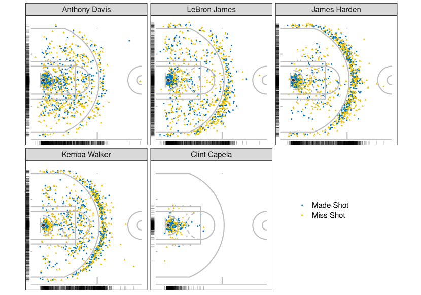
Figure 1: Shot charts for selected NBA players.

Table 1: Number of blocks corresponding to number of shots for selected players.

Observed Value	Davis	James	Harden	Walker	Capela
0	836	788	853	837	1123
1	161	212	149	159	25
2	88	91	69	82	8
3	38	35	31	35	2
4	18	16	23	17	4
5	9	8	5	9	0
6+	25	25	45	36	13

3 Methodology

3.1 Zero Inflated Poisson Regression

In this section, we briefly discuss the zero-inflated Poisson distribution (ZIP). There are some models are capable of dealing with excess zero counts (Mullahy, 1986; Lambert, 1992), and zero-inflated models are one type of them. Zero-inflated models are two-component mixture models that combine a count component and a point mass at zero with a count distribution such as Poisson, geometric or negative binomial (see, Cameron and Trivedi, 2005, for a discussion). We denote the observed count values of the $i$-th player as $\bm{y}_{i}=\left(y_{i1},y_{i2},\ldots,y_{i,1175}\right)^{\top}$. Hence, the probability distribution of the ZIP random variable $y_{ij}$ can be written as, for a nonnegative integer $\kappa$,

$$\mbox{pr}(y_{ij}=\kappa)=\begin{cases}\rho_{i}+\left(1-\rho_{i}\right)\exp{-\mu_{ij}}&\text{if $\kappa=0$}\\ \left(1-\rho_{i}\right)\frac{\mu_{ij}^{y_{ij}}\exp{-\mu_{ij}}}{y_{ij}!}&\text{if $\kappa>0$}\end{cases},$$ (1)

where $\rho_{i}$ is the probability of extra zeros and $\mu_{ij}$ is the mean parameter of Poisson distribution. For the rest of the paper, we denote this distribution as $\mbox{ZIP}(\mu_{ij},\rho_{i})$. It can be seen from (1) that ZIP reduces to the standard Poisson model when $\rho_{i}=0$. Also, we know that $\mbox{pr}(y_{ij}=0)>\exp{-\mu_{ij}}$ indicates zero-inflation. The mean parameter $\mu_{ij}$ is linked to the explanatory variables through log links as

$$\log\left(\mu_{ij}\right)=\bm{x}_{j}^{\top}\bm{\beta}_{i},$$

where $\bm{x}_{j}$ is a vector of covariates $\bm{x}_{j}=\left(1,x_{1,j},\ldots,x_{p,j}\right)^{\top}$ and $\bm{\beta}_{i}=\left(\beta_{0i},\beta_{1i},\ldots,\beta_{pi}\right)^{\top}$ are the corresponding regression coefficients including the intercept $\beta_{0i}$.

3.2 Non-Negative Matrix Factorization for Spatial Basis

To capture shot styles of individual players, following Jiao et al. (2020a), we construct spatial basis functions using historical data. Shot data for a total of 359 players who made over 100 shots in regular season 2016–2017 is used as input. First, kernel density estimation is employed to estimate the shooting frequency matrix $\bm{\lambda}=(\lambda_{1},\ldots,\lambda_{1175})$ for each individual player. Similar checking of empirical correlation between the kernel density values on blocks on the court is performed as in Miller et al. (2014), and the existence of long-range correlations in non-stationary patterns motivates the usage of a basis construction method that captures such long range correlation via global spatial patterns. This need motivates the usage of non-negative matrix factorization (NMF; Sra and Dhillon, 2005) in our modeling effort.

NMF is a dimensionality reduction technique that assumes a matrix $\bm{\Lambda}$ can be approximated by the product of two low-rank matrices

$$\bm{\Lambda}\approx\bm{W}\bm{B},$$

where the matrix $\bm{\Lambda}\in\mathbb{R}_{+}^{N\times V}$ is composed of $N$ data points of length $V$, the basis matrix $\bm{B}\in\mathbb{R}_{+}^{K\times V}$ is composed of $K$ basis vectors, and the weight matrix $\bm{W}\in\mathbb{R}_{+}^{N\times K}$ is composed of the $N$ non-negative weight vectors that scale and linearly combine the basis vectors to reconstruct $\bm{\Lambda}$. The matrices $\bm{W}$ and $\bm{B}$ are obtained by minimizing certain divergence criteria (e.g. Kullback–Leibler divergence, or Euclidean distance), with the constraint that all matrix elements remain non-negative. With the non-negativity restriction for both the weight vectors and basis vectors, NMF eliminates redundant cases where negative bases “cancel out” positive bases. The basis left is often more sparse, and focuses on partial representations, which can be combined to represent the whole story (Lee and Seung, 1999).

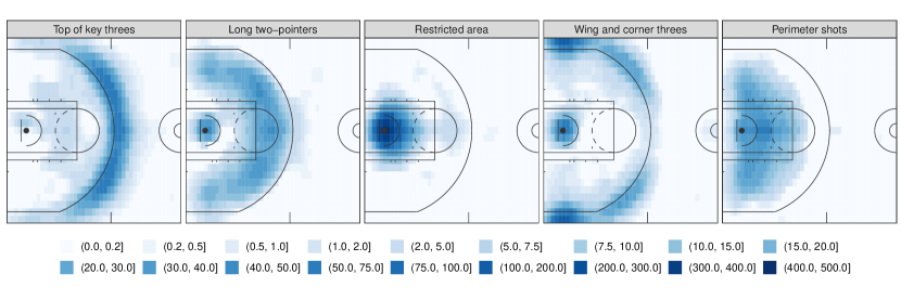
Figure 2: Visualization of basis functions obtained by NMF for $K=5$. Each basis function represents the intensity function of a particular shot type.

In our application, with data for the 359 players as a $359\times 1175$ matrix, we use the R package NMF (Gaujoux and Seoighe, 2010) to obtain $K=5$ bases, each of which correspond to a certain shot type, as illustrated in Figure 2. These five bases correspond to, respectively, top of key threes, long two-pointers, restricted area, wing and corner threes and perimeter shots. A player’s shooting habit can be approximated by a weighted combination of these bases. Nevertheless, looking at the scales, one can see that the maximum value is over 400, and the values are highly skewed. Natural logarithm of the basis values is taken to reduce extreme values, and a normalization step is subsequently performed so that values in each basis vector have mean 0 and standard deviation 1. When such normalized basis functions are used as covariates in modeling individual player’s shots, their corresponding coefficients, or weight vectors, can be regarded as a characterization for the shooting style of a player.

3.3 ZIP with Clustered Regression Coefficients

Consider a zero inflated Poisson regression model with varying coefficients as follows,

$$y_{ij}\sim\text{ZIP}\left(\exp(\bm{x}_{j}^{\top}\bm{\beta}_{i}),\rho_{i}\right),\quad i=1,\ldots,n,\quad j=1,\ldots,J.$$ (2)

where $\bm{\beta}_{i}$ is a $p+1$-dimensional regression coefficients. From Gelfand et al. (2003), a Gaussian process prior can be assigned on regression coefficients to obtain varying patterns. Assuming the existence of clusters in $\bm{\beta}$ and $\rho$, and denote the true cluster label for player $i$ as $z_{i}$, the parameters for cluster $i$ as $\bm{\beta}_{z_{i}}$ and $\rho_{z_{i}}$, then the model in (2) can be rewritten as

$$y_{ij}\sim\text{ZIP}\left(\exp(\bm{x}_{j}^{\top}\bm{\beta}_{z_{i}}),\rho_{z_{i}}\right),\quad i=1,\ldots,n,\quad j=1,\ldots,J.$$ (3)

where $z_{i}\in\left\{1,\ldots,k\right\}$, with $k$ being the total number of clusters.

One popular way to model the joint distribution of $z_{1},\ldots,z_{k}$ is the Chinese restaurant process (CRP; Blackwell et al., 1973), which defines a series of conditional distributions, also know as the a Pólya urn scheme, as:

$$P(z_{i}=c\mid z_{1},\ldots,z_{i-1})\propto\begin{cases}\absolutevalue{c},&\text{at an existing table labeled}\,c\\ \alpha,&\text{if}\,$c$\,\text{is a new table}\end{cases},$$ (4)

where $\absolutevalue{c}$ is the number of elements in cluster $c$. Despite its favorable property as a method to simultaneously estimate the number of clusters and the clustering configuration, it has proved to produce extraneous clusters in the posterior, even when the number of sample size goes to infinity, which renders the estimation for number of clusters inconsistent (Miller and Harrison, 2018). A slowed-down version of the CRP in terms of producing new tables, mixture of finite mixtures (MFM; Miller and Harrison, 2018) is proposed to mitigate this problem:

$$k\sim p(\cdot),\quad(\pi_{1},\ldots,\pi_{k})\mid k\sim\mbox{Dir}(\gamma,\ldots,\gamma),\quad z_{i}\mid k,\pi\sim\sum_{h=1}^{k}\pi_{h}\delta_{h},\quad i=1,\ldots,n,$$ (5)

where $p(\cdot)$ is a proper probability mass function on $\{1,2,\ldots,\}$ and $\delta_{h}$ is a point-mass at $h$. Compared to the CRP, the introduction of new tables is slowed down by the factor $V_{n}(t+1)/V_{n}(t)$, which allows for a model-based pruning of the tiny extraneous clusters. The coefficient $V_{n}(t)$ is precomputed as

$$\begin{split}V_{n}(t)&=\sum_{n=1}^{+\infty}\dfrac{k_{(t)}}{(\gamma k)^{(n)}}p(k),\end{split}$$

where $k_{(t)}=k(k-1)\ldots(k-t+1)$, and $(\gamma k)^{(n)}={\gamma k}(\gamma k+1)\ldots(\gamma k+n-1)$. The conditional distributions of $z_{i},i=2,\ldots,n$ under (5) can be defined in a Pólya urn scheme similar to CRP:

$$P(z_{i}=c\mid z_{1},\ldots,z_{i-1})\propto\begin{cases}\absolutevalue{c}+\gamma,&\text{at an existing table labeled}\,c\\ V_{n}(t+1)/V_{n}(t)\gamma,&\text{if}\,c\,\text{is a new table}\end{cases},$$ (6)

with $t$ being the number of existing clusters. Adapting MFM to our model setting for clustering, the model and prior can be expressed hierarchically as:

$$\begin{split}&y_{ij}\sim\text{ZIP}\left(\exp(\bm{x}_{j}^{\top}\bm{\beta}_{z_{i}}),\rho_{z_{i}}\right),\quad i=1,\ldots,n,\quad j=1,\ldots,J,\\ &\bm{\beta}_{h}\sim\text{N}\left(\textbf{0},\Sigma_{0}\right),\qquad h=1,\ldots,k,\\ &\rho_{h}\sim\text{U}\left(0,1\right),\qquad h=1,\ldots,k,\\ &z_{i}\mid k,\pi\sim\sum_{h=1}^{k}\pi_{h}\delta_{h},\\ &(\pi_{1},\ldots,\pi_{k})\mid k\sim\mbox{Dir}(\gamma,\ldots,\gamma),\\ &k\sim p(\cdot),\end{split}$$ (7)

where $p(\cdot)$ is a $\mbox{Poisson}(\psi)$ distribution truncated to be positive through the rest of the paper, which has been proved by Miller and Harrison (2018) and Geng et al. (2019) to guarantee consistency for the mixing distribution and the number of groups, $\gamma=1$, $\delta_{h}$ denotes the Dirac measure, and $\Sigma_{0}$ is hyperparameter for base distribution of $\bm{\beta}$’s. We refer to the hierarchical model above as MFM-ZIP.

3.4 Theoretical Property

In this section, we study the theoretical property of MFM-ZIP. We assume that the parameter space $\bm{\Theta^{*}}$ is the compact parameter space for all the model parameters (i.e., mixture weights, regression coefficients and zero inflated probability) given a fixed number of clusters. The mixing measure is $G=\sum_{i=1}^{k}\pi_{i}\delta_{\theta_{i}}$, where $\delta$ is the point mass measure, and $\theta_{h}=\{\bm{\beta}_{h},\rho_{h}\}$ is the collection of regression coefficients and zero inflation probability in cluster $h$ for $h=1,\ldots,k$.

Let $K_{0}$, $G_{0}$, $P_{0}$ be the true number of clusters, the true mixing measure, and the corresponding probability measure, respectively. Then the following proposition establishes the posterior consistency and contraction rate for the cluster number $K$ and mixing measure $G$. The proof is based on the general results for Bayesian mixture models in Guha et al. (2020).

Proposition 1

Let $\Pi_{n}(\cdot\mid\bm{y}_{1},\ldots,\bm{y}_{n})$ be the posterior distribution obtained from given a random sample $\bm{y}_{1},\ldots,\bm{y}_{n}$. Assume that the parameters of interest are restricted to a compact space $\bm{\Theta^{*}}$. Then we have

$$\Pi_{n}(K=K_{0}\mid\bm{y}_{1},\ldots,\bm{y}_{n})\rightarrow 1,~{}\text{and}~{}~{}\Pi_{n}(W(G,G_{0})\lesssim(\log n/n)^{-1/2}\mid\bm{y}_{1},\ldots,\bm{y}_{n})\rightarrow 1,$$

almost surely under $P_{0}$ as $n\rightarrow\infty$, where $W$ is Wasserstein distance.

Proposition 1 shows that our proposed Bayesian method is able to correctly identify the unknown number of clusters and the latent clustering structure with posterior probability tending to one as the number of observations increases.

In order to prove the Proposition 1, we need to verify the conditions (P.1)–(P.4) in Guha et al. (2020) hold. Condition (P.1) is satisfied since we restrict our parameters of interest to a compact space $\bm{\Theta^{*}}$ and uniform distribution and multivariate normal distribution are first-order identifiable. Condition (P.2) also holds since we assign an non-zero continuous prior on $\bm{\beta}$’s and $\rho$’s on the parameters within a bounded support. Uniform distribution and multivariate normal distribution is sufficient for Condition (P.3). Condition (P.4) holds since we choose a truncated Poisson distribution on $q(\cdot)$. The proof can be finished by using the results in Theorem 3.1 of Guha et al. (2020)

4 Bayesian Inference

For the hierarchical ZIP model with MFM introduced in (7), the set of parameters is denoted as $\Theta=\{(\bm{\beta}_{i},\rho_{i},z_{i},\bm{\pi},k):i=1,\cdots,n\}$. If we choose $(k-1)\sim\mbox{Poisson}(\psi)$ and $\gamma=1$ in (5), the mixture weights $\pi_{1},\cdots,\pi_{k}$ can be constructed following stick-breaking (Sethuraman, 1994) approximation:

• Step 1. Generate $\eta_{1},\eta_{2},\cdots\overset{\text{iid}}{\sim}\text{Exp}(\psi)$,

• Step 2. $k=\min\{j:\sum_{k=1}^{j}\eta_{k}\geq 1\}$,

• Step 3. $\pi_{h}=\eta_{h}$, for $h=1,\cdots,k-1$,

• Step 4. $\pi_{k}=1-\sum_{h=1}^{k-1}\pi_{h}$.

Prior for the hyperparameter $\psi$ is $\text{Gamma}(1,1)$. With the prior distributions specified above, the posterior distribution of these parameters based on the data $D=\{\bm{y}_{i},\bm{x}_{j}:i=1,\cdots,n,j=1,\cdots,p\}$ is given by

$$\pi(\Theta\mid D) \propto L(\Theta\mid D)\pi(\Theta)$$

$$=\prod_{i=1}^{n}f(\bm{y}_{i},\bm{x}_{1},\ldots,\bm{x}_{j}\mid\bm{\beta}_{z_{i}},\rho_{z_{i}},z_{i})\pi(\Theta),$$

where $\pi(\Theta)$ is the joint prior for all the parameters. Due to the unavailability of the analytical form for the posterior distribution of $\Theta$, we employ the MCMC sampling algorithm to sample from the posterior distribution, and then obtain the posterior estimates of the unknown parameters. Computation is facilitated by the nimble(de Valpine et al., 2017) package in R (R Core Team, 2013). The implementation code is given in supplementary materials at https://ys-xue.github.io/MFM-ZIP-Basketball-Supplemental/. Another important task is to do the posterior inference for clustering labels. We carry out posterior inference on the clustering labels based on Dahl’s method (Dahl, 2006), which proceeds as follows,

• Step 1. Define membership matrices $\mathcal{A}^{(t)}=(\mathcal{A}^{(t)}(i,j))_{i,j\in\left\{1,\ldots,n\right\}}=(\bm{1}(z_{i}^{(t)}=Z_{j}^{(t)}))_{n\times n}$, where $t=1,\ldots,T$ is the index for the retained MCMC draws after burn-in, and $\bm{1}(\cdot)$ is the indicator function.

• Step 2. Calculate the element-wise mean of the membership matrices over MCMC draws $\overline{\mathcal{A}}=\frac{1}{T}\sum_{t=1}^{T}\mathcal{A}^{(t)}$.

• Step 3. Identify the most representative posterior $\overline{\mathcal{A}}$ draw based on minimizing the element-wise Euclidean distance $\sum_{i=1}^{n}\sum_{j=1}^{n}(\mathcal{A}^{(t)}(i,j)-\overline{\mathcal{A}}(i,j))^{2}$ among the retained $t=1,\ldots,T$ posterior draws.

The posterior estimates of cluster memberships $z_{1},\ldots,z_{n}$ and other model parameters $\bm{\beta}$’s and $\rho$’s can be also obtained using Dahl’s method accordingly.

5 Simulation Study

5.1 Simulation Setup

We have two scenarios in our simulation, balanced type and imbalanced type. A total of 75 players are separated to three different groups for each type. Under the balanced design, each group contains equal number of players. Under the imbalanced design, the group sizes are 10, 35 and 30, respectively. The spatial domain is the same as for the motivating data in Section 2. We generate data $\{y_{i,j};~{}\forall i=1,\ldots,75;j=1,\ldots,1175\}$ from ZIP model with different mean parameter and probability parameter of extra zeros. In our simulation setting, our covariates contains an intercept term and five basis function terms (see Section 3.2). Different values of coefficient $\bm{\beta}$ are used: $\left(-1,1.2,0.95,1.1,1,0.8\right)^{\top}$, $\left(-0.4,0.6,0.7,0.5,0.8,0.3\right)^{\top}$, and $\left(-0.9,0.2,0.1,0.3,0.2,0.4\right)^{\top}$, corresponding to each cluster respectively. We set the true probability parameter of extra zeros for each cluster to be $\left(0.1,0.3,0.4\right)$.

We examine both the estimation for number of groups as well as congruence of group belongings with the true setting in terms of modulo labeling by Rand index (RI; Rand, 1971), the computation of which is facilitated by the R-package fossil (Vavrek, 2011). The RI ranges from 0 to 1 with a higher value indicating better agreement between a grouping scheme and the true setting. In particular, a value of 1 indicates perfect agreement.

5.2 Simulation Results

We run our algorithm with 7,000 MCMC iterations, with the first 2,000 iterations as burn-in for each replicate. The chain length has been examined to ensure convergence and stabilization. Proceeding to 100 separate replicates of data, our proposed algorithm was run, and 100 RI values are obtained by comparing with the true setting. We calculate cover rate for both scenario. For each scenario, we also calculate the cover rate, which equals the percentage of replicates that our proposed algorithm accurately recovers the true number of clusters. The cover rate for each scenario are 98% and 93%, respectively. We also compare our method to $K$-means algorithm, high dimensional supervised classification and clustering (hdc; Bergé et al., 2012, R-package HDclassif) and mean shift grouping. The mean shift algorithm is a steepest ascent classification algorithm, where classification is performed by fixed point iteration to a local maxima of a kernel density estimate. This method is originally from Fukunaga and Hostetler (1975), and an implementation in R can be found in the meanShiftR package (Lisic, 2018). Grouping recovery performances of all four methods are measured using the RI. As $K$-means and the mean shift algorithm cannot infer the number of clusters, such values need to be pre-specified, and we supply them with the number of clusters inferred by our method in each replicate. The clustering performances are compared in Table 2. In both designs, our proposed method have the highest RI, indicating its high accuracy in clustering. $K$-means and hdc have RI greater than 0.9, but the average performance is not as good as the proposed model. The mean shift algorithm, however, yields the worst performance.

We provide parameter estimation in Table 3. For each of the three $\bm{\beta}$’s, the average parameter estimate denoted by $\bar{\widehat{\beta}}_{\ell,m}$ $\left(\ell=1,\ldots,75;m=1,\ldots,6\right)$ in 100 simulations is calculated as

$$\bar{\widehat{\beta}}_{\ell,m}=\frac{1}{100}\sum_{r=1}^{100}\widehat{\beta}_{\ell,m,r}$$

where $\widehat{\bm{\beta}}_{\ell,m,r}$ denotes the posterior estimate for the $m$-th coefficient of player $\ell$ in the $r$-th replicate. We use different metrics to evaluate the posterior performance. Those metrics including the mean absolute bias (MAB), the mean standard deviation (MSD), the mean of mean squared error (MMSE) and mean coverage rate (MCR) of the 95% highest posterior density (HPD) intervals in the following ways:

MAB $$=\frac{1}{75}\sum_{\ell=1}^{75}\frac{1}{100}\sum_{r=1}^{100}\absolutevalue{\widehat{\beta}_{\ell,m,r}-\beta_{\ell,m}},$$

MSD $$=\frac{1}{75}\sum_{\ell=1}^{75}\sqrt{\frac{1}{99}\sum_{r=1}^{100}\left(\widehat{\beta}_{\ell,m,r}-\bar{\widehat{\beta}}_{\ell,m}\right)^{2}},$$

MMSE $$=\frac{1}{75}\sum_{\ell=1}^{75}\frac{1}{100}\sum_{r=1}^{100}\left(\widehat{\beta}_{\ell,m,r}-\beta_{\ell,m}\right)^{2},$$

MCR $$=\frac{1}{75}\sum_{\ell=1}^{75}\frac{1}{100}\sum_{r=1}^{100}1_{\left\{\widehat{\beta}_{\ell,m,r}\in\text{95\% HPD interval}\right\}},$$

where $1_{\{\}}$ denotes the indicator function. The four metrics for each $\beta$ under the balanced and imbalanced designs are presented in Table 3. With high clustering accuracy as indicated by the RI, the estimated $\bm{\beta}$ for each cluster is close to its corresponding true value, which can be reflected by the small numerical values in the MAB column. The estimation performance is stable, in the sense that the MSD values are also small. The MCR under the balanced design fluctuate around its nominal value of 0.95, and under the imbalanced design, the values are overall lower due to the influence of mis-clustered players, but still remain close to or greater than 0.9.

Table 2: Comparison of clustering performance for the proposed method and three other competing approaches.

Type	Cover Rate	$\text{RI}_{\mbox{mfm}}$	$\text{RI}_{\mbox{kmeans}}$	$\text{RI}_{\mbox{hdc}}$	$\text{RI}_{\mbox{meanshift}}$
Balanced	98%	0.9955	0.9364	0.9344	0.6757
Imbalanced	93%	0.9836	0.9581	0.9735	0.6126

Table 3: Performance of parameter estimates under the two true cluster designs.

Type		MAB	MSD	MMSE	MCR
Balanced	$\beta_{0}$	0.01610	0.0421	0.001930	0.933
	$\beta_{1}$	0.01340	0.0322	0.001060	0.927
	$\beta_{2}$	0.01190	0.0279	0.000884	0.943
	$\beta_{3}$	0.00928	0.0272	0.000788	0.960
	$\beta_{4}$	0.01150	0.0266	0.000904	0.930
	$\beta_{5}$	0.00920	0.0235	0.000604	0.920
Imbalanced	$\beta_{0}$	0.02680	0.0663	0.005950	0.901
	$\beta_{1}$	0.02340	0.0521	0.003160	0.911
	$\beta_{2}$	0.02030	0.0504	0.002790	0.896
	$\beta_{3}$	0.01880	0.0424	0.002360	0.921
	$\beta_{4}$	0.01960	0.0491	0.002790	0.916
	$\beta_{5}$	0.01740	0.0380	0.001770	0.912

6 Real Data Application

In this section, we apply the proposed method to the analysis of players’ shot data in the 2017-2018 NBA regular season. Only the locations of shots are considered regardless of the player’s positions on the court (e.g., point guard, power forward, etc.). We run 15,000 MCMC iterations and the first 5,000 iterations as burn-in period. The result from the MFM-ZIP model suggests that the 191 players are to be classified into four groups. The sizes of the four groups are 29, 110, 48 and 4 respectively. We visualize the shot attempt counts made by four selected players on blocks of the court in Figure 3. The players for each group are shown in Section 3 of the supplementary materials.

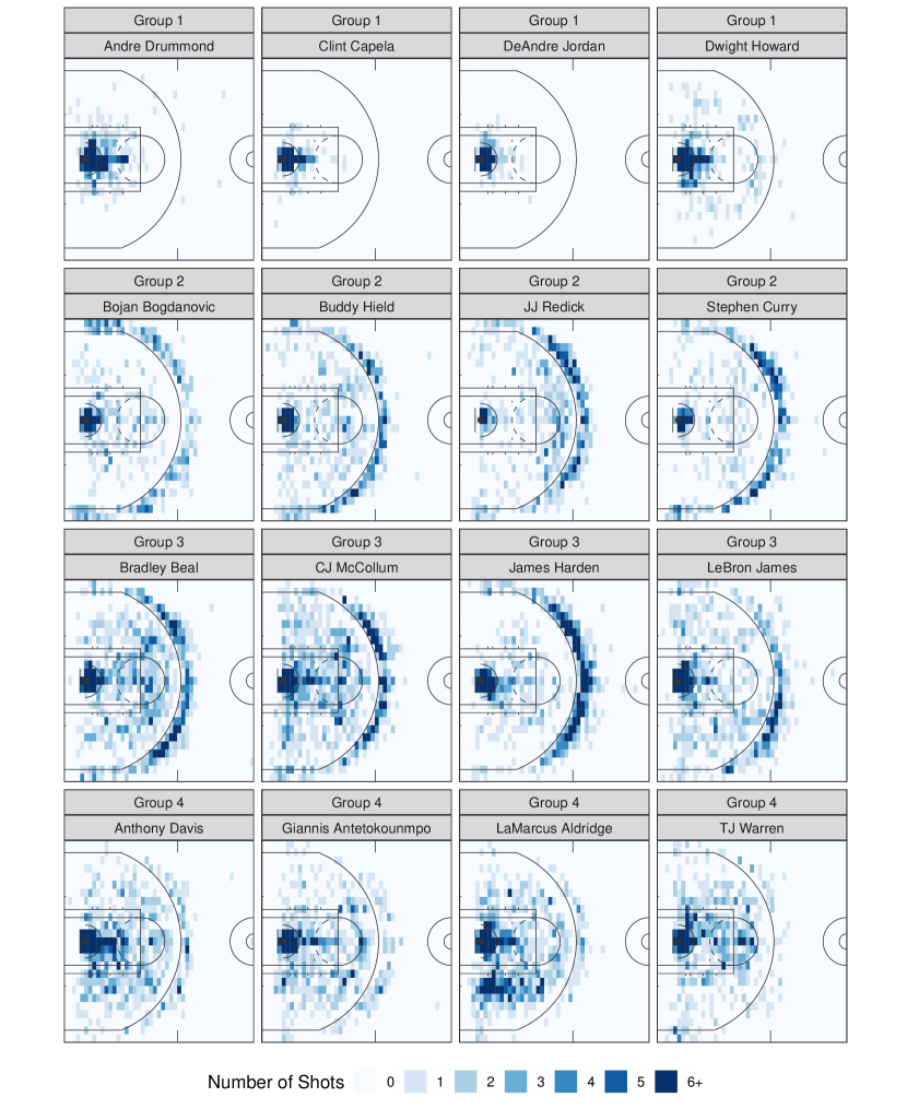
Figure 3: Visualization of shooting patterns for four selected players from each group.

Table 4: Performance of parameter estimates under the real data.

	$\rho$	$\beta_{0}$	$\beta_{1}$	$\beta_{2}$	$\beta_{3}$	$\beta_{4}$	$\beta_{5}$
Group 1	0.583	-1.857	0.256	0.573	1.374	0.531	1.061
Group 2	0.618	-0.409	0.731	0.200	0.359	0.581	0.392
Group 3	0.515	-0.147	0.511	0.237	0.505	0.493	0.474
Group 4	0.322	-1.205	0.258	1.101	1.056	0.426	0.766

Several interesting observations can be made from Figure 3. It can be seen that each group of players has their own favorite shooting locations. Players in Group 1 make the most shots neat the hoop, which is confirmed by the regression coefficients in Table 4 as their coefficients for the third and fifth basis functions are the largest. Clint Capela and DeAndre Jordan, for example, are both good at making alley-oops and slam dunks. Andre Drummond and Dwight Howard are also centers who rarely leave the painted area.

Players in Group 2 make the most shots beyond the three-point line, as they have the largest parameter estimates for the first and fourth basis function when compared to other groups. As shown in Figure 3, JJ Redick and Stephen Curry are both well-known shooters.

A first look at the plots for Group 3 indicates that players in this group are able to make all types of shots, including three-pointers, perimeter shot, and also shots over the painted area. We find the players in this groups are often the leaders in their teams, and usually have the most posession. The parameter estimates also confirm the observation. Their $\widehat{\beta}_{0}$ is the largest among all groups, indicating an overall higher probability for making shots. Compared with Group 2, their shots are more evenly distributed, which can be reflected by the larger parameter estimate for the basis functions corresponding to areas within the three-point line.

For Group 4, we find that most of their shots are close to the hoop and around the perimeter, and they have fewer shot around or beyond the three-point line. From the estimation result, the coefficient for the second and third basis functions are larger than other basis functions, and similar in value. In addition, their $\widehat{\beta}_{1}$ is the second smallest among all four groups while $\widehat{\beta}_{4}$ is the smallest, which again indicates their disfavor of shooting beyond the three-point line. Note that the presented analysis is based on 2017–2018 regular season, which was before Giannis Antetokoumpo increased his three-point shots in the 2019–2020 season.

7 Discussion

Based on theoretical justifications and empirical studies, our proposed methods successfully solve the three challenges raised in Section LABEL:sec:intro. Based on the results shown in Section 5, our proposed methods accurately estimates the parameters in the ZIP model and recovers the number of clusters and clustering configurations with different proportions of zero counts. Compared with several benchmark clustering methods such as $K$-means, high dimensional supervised classification and clustering, and mean shift grouping, our methods have higher clustering concordance without any tuning steps.

In the analysis of the NBA shot charts data, four field goal attempt patterns, their corresponding zero inflation probabilities, and regression coefficients of each group are identified. The results provide valuable insights to players, coaches, and managers. The players can obtain more descriptive analysis of their current offense patterns, and hence develop customized training plans with pertinence; the coaches can organize their offense and defense strategies more efficiently for different opponents; the mangers will make better data-informed decisions on player recruiting and trading during offseason.

There are several possible directions for further investigation. Spatial correlation over the court is accounted for nonparametrically by the basis functions. Considering either stationary or nonstationary model-based spatial correlation in our proposed modeling framework is a natural extension. In this paper, our posterior sampling is based on stick-breaking representations. Developments of more scalable inference algorithms (e.g., variational inference) are critical for large scale data. Finally, building a heterogeneity learning model with auxiliary information from different players, such as age and position on the court, merits future research from both methodological and applied perspectives.

References

- Bergé et al. (2012) Bergé, L., C. Bouveyron, and S. Girard (2012). HDclassif: An R package for model-based clustering and discriminant analysis of high-dimensional data. Journal of Statistical Software 46(6), 1–29.
- Blackwell et al. (1973) Blackwell, D., J. B. MacQueen, et al. (1973). Ferguson distributions via Pólya urn schemes. The Annals of Statistics 1(2), 353–355.
- Cameron and Trivedi (2005) Cameron, A. C. and P. K. Trivedi (2005). Microeconometrics: Methods and Applications. Cambridge university press.
- Dahl (2006) Dahl, D. B. (2006). Model-based clustering for expression data via a Dirichlet process mixture model. In M. V. Kim-Anh Do, Peter Müller (Ed.), Bayesian Inference for Gene Expression and Proteomics, Volume 4, pp. 201–218. Cambridge University Press.
- de Valpine et al. (2017) de Valpine, P., D. Turek, C. J. Paciorek, C. Anderson-Bergman, D. T. Lang, and R. Bodik (2017). Programming with models: writing statistical algorithms for general model structures with NIMBLE. Journal of Computational and Graphical Statistics 26(2), 403–413.
- Ferguson (1973) Ferguson, T. S. (1973). A Bayesian analysis of some nonparametric problems. The Annals of Statistics 1(2), 209–230.
- Fukunaga and Hostetler (1975) Fukunaga, K. and L. Hostetler (1975). The estimation of the gradient of a density function, with applications in pattern recognition. IEEE Transactions on information theory 21(1), 32–40.
- Gaujoux and Seoighe (2010) Gaujoux, R. and C. Seoighe (2010). A flexible R package for nonnegative matrix factorization. BMC bioinformatics 11(1), 367.
- Gelfand et al. (2003) Gelfand, A. E., H.-J. Kim, C. Sirmans, and S. Banerjee (2003). Spatial modeling with spatially varying coefficient processes. Journal of the American Statistical Association 98(462), 387–396.
- Geng et al. (2019) Geng, J., A. Bhattacharya, and D. Pati (2019). Probabilistic community detection with unknown number of communities. Journal of the American Statistical Association 114(526), 893–905.
- Geyer (1998) Geyer, C. (1998). Likelihood inference for spatial point processes. In W. S. Kendall (Ed.), Stochastic Geometry: Likelihood and Computation, Volume 80, pp. 79. CRC Press.
- Goulard et al. (1996) Goulard, M., A. Särkkä, and P. Grabarnik (1996). Parameter estimation for marked Gibbs point processes through the maximum pseudo-likelihood method. Scandinavian Journal of Statistics 23(3), 365–379.
- Guha et al. (2020) Guha, A., N. Ho, and X. Nguyen (2020). On posterior contraction of parameters and interpretability in Bayesian mixture modeling. Bernoulli. Forthcoming.
- Hu et al. (2019) Hu, G., F. Huffer, and M.-H. Chen (2019). New development of Bayesian variable selection criteria for spatial point process with applications. arXiv preprint arXiv:1910.06870.
- Hu et al. (2020) Hu, G., H.-C. Yang, and Y. Xue (2020). Bayesian group learning for shot selection of professional basketball players. Stat, e324.
- Jiao et al. (2020a) Jiao, J., G. Hu, and J. Yan (2020a). A Bayesian joint model for spatial point processes with application to basketball shot chart. Journal of Quantitative Analysis in Sports. Forthcoming.
- Jiao et al. (2020b) Jiao, J., G. Hu, and J. Yan (2020b). Heterogeneity pursuit for spatial point pattern with application to tree locations: A Bayesian semiparametric recourse. arXiv preprint arXiv:2003.10043.
- Lambert (1992) Lambert, D. (1992). Zero-inflated Poisson regression, with an application to defects in manufacturing. Technometrics 34(1), 1–14.
- Lee and Seung (1999) Lee, D. D. and H. S. Seung (1999). Learning the parts of objects by non-negative matrix factorization. Nature 401(6755), 788–791.
- Lisic (2018) Lisic, J. (2018). meanShiftR: A Computationally Efficient Mean Shift Implementation. R package version 0.53.
- Miller et al. (2014) Miller, A., L. Bornn, R. Adams, and K. Goldsberry (2014). Factorized point process intensities: A spatial analysis of professional basketball. In E. P. Xing and T. Jebara (Eds.), Proceedings of the 31st International Conference on Machine Learning, Volume 32 of Proceedings of Machine Learning Research, Bejing, China, pp. 235–243. PMLR.
- Miller and Harrison (2018) Miller, J. W. and M. T. Harrison (2018). Mixture models with a prior on the number of components. Journal of the American Statistical Association 113(521), 340–356.
- Møller et al. (1998) Møller, J., A. R. Syversveen, and R. P. Waagepetersen (1998). Log Gaussian Cox processes. Scandinavian Journal of Statistics 25(3), 451–482.
- Mullahy (1986) Mullahy, J. (1986). Specification and testing of some modified count data models. Journal of Econometrics 33(3), 341–365.
- R Core Team (2013) R Core Team (2013). R: A Language and Environment for Statistical Computing. Vienna, Austria: R Foundation for Statistical Computing.
- Rand (1971) Rand, W. M. (1971). Objective criteria for the evaluation of clustering methods. Journal of the American Statistical Association 66(336), 846–850.
- Reich et al. (2006) Reich, B. J., J. S. Hodges, B. P. Carlin, and A. M. Reich (2006). A spatial analysis of basketball shot chart data. The American Statistician 60(1), 3–12.
- Sethuraman (1994) Sethuraman, J. (1994). A constructive definition of Dirichlet priors. Statistica Sinica, 639–650.
- Sra and Dhillon (2005) Sra, S. and I. Dhillon (2005). Generalized nonnegative matrix approximations with bregman divergences. Advances in neural information processing systems 18, 283–290.
- Vavrek (2011) Vavrek, M. J. (2011). fossil: palaeoecological and palaeogeographical analysis tools. Palaeontologia Electronica 14(1), 1T. R package version 0.4.0.
- Yin et al. (2020) Yin, F., G. Hu, and W. Shen (2020). Analysis of professional basketball field goal attempts via a bayesian matrix clustering approach. arXiv preprint arXiv:2010.08495.
- Yin et al. (2020) Yin, F., J. Jiao, G. Hu, and J. Yan (2020). Bayesian nonparametric estimation for point processes with spatial homogeneity: A spatial analysis of NBA shot locations. arXiv preprint arXiv:2011.11178.
- Zhao et al. (2020) Zhao, P., H.-C. Yang, D. K. Dey, and G. Hu (2020). Bayesian spatial homogeneity pursuit regression for count value data. arXiv preprint arXiv:2002.06678.