Probabilistic Conditional System Invariant Generation with Bayesian Inference

Abstract

Invariants are a set of properties over program attributes that are expected to be true during the execution of a program. Since developing those invariants manually can be costly and challenging, there are a myriad of approaches that support automated mining of likely invariants from sources such as program traces. Existing approaches, however, are not equipped to capture the rich states that condition the behavior of autonomous mobile robots, or to manage the uncertainty associated with many variables in these systems. This means that valuable invariants that appear only under specific states remain uncovered. In this work we introduce an approach to infer conditional probabilistic invariants to assist in the characterization of the behavior of such rich stateful, stochastic systems. These probabilistic invariants can encode a family of conditional patterns, are generated using Bayesian inference to leverage observed trace data against priors gleaned from previous experience and expert knowledge, and are ranked based on their surprise value and information content. Our studies on two semi-autonomous mobile robotic systems show how the proposed approach is able to generate valuable and previously hidden stateful invariants.

I Introduction

Our community has built a large body of work on likely invariant generation from system traces. This body includes the inference of invariants of different types [22], from those attempting to characterize a variable range of values [5, 4, 13, 16, 21] to those infering temporal invariants [11, 18, 19, 20, 25, 2, 27]. The body of work also utilizes a variety of inference mechanisms ranging from frequentist inference [4] to the generation of polynomial relations [21] to k-tail [19] to deep learning [18]. As we explored this body of work for its application to autonomous mobile robots, however, we came to realize that these kinds of systems introduce a couple of unique attributes that existing invariant generation approaches were unable to fully capture.

The first unique attribute is the extent to which different system states render distinct sets of invariants, as the behavior of these systems is conditioned not so much by typical programmatic structures (i.e., functions’ pre- and post-conditions), but rather by particular system states. For example, the sensors activated and the attitude of a drone are conditioned by different mission states such as takeoff, approaching a target, or tracking a target, while a self-driving vehicle’s linear velocity bounds may change depending on whether the car is charging, parking, driving within a city, or driving on a highway. We argue and later show that ignoring this attribute greatly limits the potential of uncovering valuable invariants that only appear under certain states.

The second distinctive attribute is the degree of uncertainty intrinsic to these systems. They may render different results under the same environmental conditions due to sensor noise, imperfect estimators, inaccurate actuators, and humans in the loop. For example, the GPS sensor of the drone’s localization component we later study has an accuracy of $\pm 3.0$ meters, the target recognition component success depends on the hovering stability which affects the camera’s ability focus, and human operators with similar training can have a wide variety of reaction times. We argue and later show that failing to handle this uncertainty attribute properly will make it difficult to judge the value of an inferred invariant.

The state of the art in invariance inference, however, does not support the generation of invariants that are conditioned by arbitrarily complex system states, nor does it support probabilistic invariants to better characterize the uncertainty associated with the exposed behaviors. The closest related work considers having two outcomes happening jointly (that is, occurring at the same time, but not conditioned on each other) and ignores the prior system probabilities by making assumptions about the data distribution [4].

In this work we address this challenge by building on the statistical structure of conditional probabilities, $Probability(Outcome|Given)$, to uncover likely invariants that only manifest under particular given program states. As we shall see, our approach generates invariants such as:

$$\begin{split}P(appliedThrotle&=0\mid\\ &vehicleMode=autonomous\quad\wedge\\ &pedestrianLocation=roadway)>0.99\\ \end{split}$$

which indicates that, given that a vehicle is operating in autonomous mode and a pedestrian is closeby, the probability for the throttle to be disengaged is over 99% (in contrast, without such conditioning, we could only learn that the Throttle range is between 0 and 100).

Problem requirements. We aim to fulfill four requirements to make the approach practical. 1) Provided with a high-level specification of the potential variables to explore as part of the $Outcome$ and $Given$, the approach must systematically investigate the space of relevant predicates to those variables as part of the $Outcomes$ that only hold under predicates on those variables as part of the $Given$. Note that such high-level specifications can be provided by an engineer or by existing invariant generation tools like the ones cited earlier. 2) The approach must enable the developer to uncover valuable conditional invariants among the large space of predicates explored. 3) The approach must be able to incrementally incorporate prior knowledge as it becomes available, either from a new collected trace or from a developer’s knowledge, to improve the probability estimates, without incurring in the cost of recomputing all invariants when new data is added. This is particularly important as multiple sources of evidence become available as the system evolves. 4) The approach must avoid relying on arbitrary thresholds to determine what is and is not significant as the choice of such thresholds is highly dependent on the context.

Conceptual Solution. To address the first requirement, we define a family of initial relevant predicates patterns for the robotics domain and a Bayesian invariant inference engine that implements conditional inference, and prototype a domain-specific specification language and a tool pipeline to compute them. To address the second requirement, we incorporate ranking mechanisms that assist in judging an invariant value based on how much an invariant probability changed from prior estimates to posterior findings. To address the third and fourth requirement, and also to further support the first requirement, we shift the inference model from using the classical (frequentist) statistics employed by existing approaches (e.g., [4, 13, 16, 27]), to a Bayesian inference model that allows us to easily incorporate prior information from previous traces or developer’s knowledge, and does not require the definition of arbitrary thesholds or the reliance on data distribution assumptions.

The contributions of this work are:

• Approach to infer a family of conditional invariants from traces through Bayesian inference, and mechanism to rank the solutions based on probabilities and surprise

• Implementation that provides the mechanisms to specify the space of variable predicates to explore, and launch the inference engine to systematically explore that space.

• Assessment of the proposed approach through its application to two systems, a reconnaissance drone and a semi-autonomous simulated car. The findings indicate that the approach can uncover valuable invariants that cannot be generated by existing approaches.

II MOTIVATING EXAMPLE

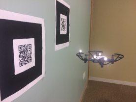
Figure 1: Drone ISR scenario.

Consider a drone performing a surveillance mission over a field whose objective is to locate and confirm a target. Figure 1 shows a downsized version of this real-world scenario where a micro-drone is sweeping for QR code targets.

This system contains a rich set of states that condition system behavior. The system state includes a large set of variables-value pairs, from the drone’s pose to its mission phase. Existing techniques [4, 11] can readily capture state invariants such as $0.0<droneAltitude<400$ as preconditions when the drone enters its navigation subroutine, or even as temporal invariants such as $\boxempty((dronePhase=Takeoff)\implies\diamond(dronePhase=Land))$.

Existing techniques, however, fail to explore the rich and valuable space of invariants that are conditioned by system states. For example, although drone altitude can change over the range of a mission, when landed, the relative drone altitude should be zero. More specifically, we want to capture the conditioned drone altitude by the phase as in $(droneAltitude=0\mid dronePhase=Land)$, effectively refining the earlier invariant on $droneAltitude$ as it is conditioned by $dronePhase$. In other cases, not just refined but totally new invariants emerge as the likelihood of the Outcome increases enough under a particular condition to be reportable. For example, since a drone’s altitude can change significantly while flying and following a trajectory, no invariants on altitude changes would be usually reported as there is no sufficient evidence to support an inference. However, the altitude of a drone should remain fairly consistent while hovering, so the $dronePhase$ conditions the altitude change as in $(|Alt_{start:hov}-Alt_{end:hov}|<\delta\mid dronePhase=Hovering)$.

Most of the mentioned states are coupled with sources of stochasticism, such as sensors affected by environmental conditions (lighting affecting target recognition capabilities), fusing estimators influenced by sensor noise (accuracy of the reported gps and pressure sensor altitude), or users variability (mission commands that are inconsistent even under the same context). As such, the conditioned and the conditioning states are inherinetly uncertain. So, while it may be correct to report that $0\leq droneSpeed\leq 5$, we would like to produce a conditional characterization that relates velocity and target recognition such as $(targetSensor=targetDetected\mid 0\leq droneSpeed\leq upperSpeed\wedge missionPhase=targetDetected)$. However, such invariant would not be that useful because for it to hold with total certainty $upperSpeed\approx 0$, which reduces the conditioning space so much that the value of the invariant decreases as it will only hold very rarely. Instead, what we envision is to be able to include larger portions of the state for invariants to be more useful but accommodate the uncertainty as part of a probability to form our proposed structure of $P(Outcome\mid Given)$. That would help us generate $P(targetSensor=targetDetected\mid 0\leq droneSpeed\leq upperSpeed=3\wedge missionPhase=targetDetected)>95$ which indicates that there is a high likelihood, over 95%, that when the drone velocity is under 3 m/s and the mission phase is target detected, the target will be sensed properly. One more distinguishing feature of the proposed approach is that to compute (and subsequently update) the probabilistic distributions associated with these outcomes, we use Bayesian inference to determine the conditional probability. As we shall see, this approach let us incorporate new traces into the inference process more efficiently and it avoids the use of artificial thresholds for reporting.

III Related Work

As mentioned in Section I, our community contribution to invariant generation has been extensive. We now decribe in more detail the work that most influenced our effort.

Ernst et. al. [4] established Daikon, one of the benchmark inference engines for detecting program invariants. Daikon’s engine creates a field of potential invariants based on a set of predefined invariant templates and a trace. We follow a similar approach in that our predicates are basic patterns, but we incorporate them in the richer conditional probability structure. Daikon then evaluates the potential invariants according to whether there are sufficient samples to support them and no samples that violate them. This frequentist approach, prevalent among invariant inference engines, uses a confidence interval to ascertain that a predicate holds against some probability of random negation, determined by the number of samples supporting that predicate. One drawback of their frequentist approach is that, while new traces can be added to an existing sufficiently large set of samples, there is a significant cost associated with trace accumulation and algorithmic complexity needed to reach that sufficiently large set without relaxing the confidence interval. Furthermore, although Daikon computes joint probabilities, it does not compute conditional invariants, nor multi-predicate joint probabilities.

Perracotta [27] extracts temporal API specifications from traces through a mix of analyses, patterns, and heuristics. Perracota was among the first to incorporate mechanisms to ignore potential blips of noisy trace content as negligible in the context of the overall trend of behavior. Our search for probabilistic invariant generation is inspired by these kinds of challenges. In a similar line of work, Gabel et al. [11] developed a mining framework of temporal logic properties. Their approach is similar to many approaches in terms of combining patterns and incrementally encoding them as FSMs. However, their strategy to start with simple patterns that can be composed to generate much more complex ones is one that we have adopted in our approach.

Grunkse [12] focuses on probabilistic invariants as a qualitative expression of requirements. He introduces a rich set of specification patterns coupled with a structured English grammar to express bounded probabilistic behavior of a system, instead of in terms of absolute correctness, to incorporate expert knowledge and for it to be used for formal verification. Although this work did not pursue automated inference of invariants, its treatment of probabilistic patterns offers a roadmap for us to expand our work.

Jiang et al. [16, 17] extend the Daikon invariant library to patterns seen in robotic systems in order to derive monitors that can check system properties at runtime. While Jiang et al. introduce invariant templates tailored to robotic systems (e.g., deployed processed and their relationship, bounded time differentials, polygonal relationships between spatial variables), their approach still relies on a traditional frequentist approach and does not considers conditionals. Aliabadi et al. [1] present a similar approach for cyberphysical system security with a focus on reduction of false positives and false negatives.

We note that none of the approaches, although closely aligned with ours, produce the conditional probabilistic invariants with Bayesian inference that we are pursuing.

IV APPROACH

The goal of the proposed approach is to generate invariants that capture the probabilistic influence between system states as in $P(Outcome|Given)$. The next sections describe how, by building on conditional probabilities and Bayesian statistical inference, we can process system traces to produce invariants that meet that goal.

IV-A Building Blocks

We capture the probabilistic influence between two dependent states as conditional probabilities of the form $P(Outcome\mid Given)$, where $Outcome$ and $Given$ are boolean predicates evaluated over single or multiple states of a system. This simple conditional pattern belies the richness of invariants it can encode, as these predicates can take many forms and can be composed to form arbitrarily complex descriptions of states.

In its simplest form, if $Given$ is TRUE, then $P(Outcome\mid Given)=P(Outcome)$. This implies that any existing invariant patterns explored in the related work or generated by existing invariants toolsets (e.g., [4, 20, 16]) can be subsumed by the proposed this encoding. That includes from the simplest form of state invariants such as $battery>0$ to complex metric temporal logic formulas such as $\boxempty(Takeoff)\implies\diamond_{[0,3]}(altitude>0))$. We also later discuss in Section IV-E the patterns that we currently support in our own infrastructure, whose selection was driven in part by the needs we observed in the robotic systems we have developed and studied.

In its richest form and the focus of this effort, $P(Outcome\mid Given)$ lets us explore how the system state encoded in $Given$ conditions the occurance of other states encoded in $Outcome$.

IV-B Bayesian Inference

The inference engine that computes $P(Outcome\mid Given)$ takes as input a space of boolean predicates to explore as part of $Outcome$ and $Given$, an execution trace of time-stamped variable-value pairs, and set of prior distributions corresponding to the prior probabilities which reflect whatever knowledge the developer has on the $Outcome$. This engine sits in the middle of a larger framework depicted in Figure 2 that we have prototyped and that is described in more detail in Section IV-E. Briefly, the configure module checks the specification of the space of predicates to explore for completeness, provides a summary of the $Outcome$ and $Given$ space to be explored, and it generates a configuration to guide the inference engine in the analysis of the traces as per those predicates. The data wrangling module preprocesses the trace to put it in the right engine format. The configuration and wrangling modules are described later in more detail.

The inference engine relies on Bayesian inference to compute conditional probabilities based on the predicate space and information in the trace and the prior. The engine produces such probability as per the Bayesian formula:

$$P(Outcome\mid Given)=\frac{P(Given\mid Outcome)P(Outcome)}{P(Given)}$$

where $P(Given\mid Outcome)$ and $P(Given)$ are computed by the engine from the trace, while $P(Outcome)$ comes from the priors. In the next section we will discuss how the generated conditional probabilities can be ranked by the posterior probabilities or by the change from the prior.

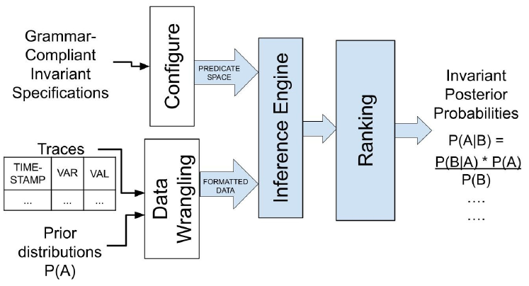
Figure 2: Approach Overview.

Algorithm 1 shows the key steps in the inference process for two predicates, $O$ in the $Outcome$ and $G$ in the $Given$, to form $P(O\mid G)$. Given a trace, those two predicates $O$ and $G$, and a prior distribution for $O$, the algorithm starts by processing each record in the trace, and evaluating the predicates on the appropriate trace variables. Such evaluation is performed according to the type of predicate to render a TRUE if the predicate holds. If predicates $O$ or $G$ hold, then their corresponding frequency count is updated, and if both of them hold then their joint probability is also updated. Once the trace is processed, these frequency counts are used to compute the probabilities required by Bayesian inference: the total probability P($G$) and the joined probablity P($G\mid O$).

The prior $P(O)$ that is provided as input to the engine can be obtained from sources such as previous deployments of the system in distint contexts, or tests results collected on variants of the system. In our studies we derive the initial priors in one of two ways: either by assuming a uniform distribution, where all values of a variable are ascribed the same probability: X $\sim$ Uni[a, b]: p(x)= $\frac{1}{b-a+1}$; or by using a disjoint subset of data as a sampling distribution arrived at by counting the observations of a certain variable value over observations of all values of that variable: X $\sim$ F${}_{x}(x_{i})$ = $\frac{freq(x_{i})}{\sum freq(x)}$. Equipped with those three probabilities, the algorithm can now finally compute P($O\mid G$). Note that as defined, Algorithm 1 operates on a single trace. In practice, building on Bayes updating, this algorithm is repeatedly invoked as new traces are collected and beliefs are refined, so that the information resulting from an analysis can be refined as more information is gathered. To accomodate new data that may affect the initial computed priors, we have incorporated a priors update step in between traces. The number of observations for each $O$ predicate and number of timesteps in the previous trace, as well as the total number of timesteps from which the previous prior was generated are propagated forward for a frequentist update of the prior probabilities in which these probability distributions of the ongoing prior and the events in the previous trace are combined by weighting the supporting observations as such:

$$Prior_{new}=\frac{Prior_{old}*timesteps_{old}+observations_{new}}{timesteps_{old}+timesteps_{new}}$$

This allows us to leverage new trace data to build a more representative prior distribution, providing increasingly accurate invariant probabilities as new trace data is consumed.

Two additional aspects of the algorithm acquire additional complexity. First, the $eval$ function must deal with predicates that require processing multiple trace records concurrently, peeking backward and forward in the trace to evaluate predicates over multiple states such as those describing a trend of values or a temporal relationship. For example, a predicate to determine whether the $acceleration$ is increasing within a time window, or a predicate that checks whether the $altitude$ eventually converges requires an analysis that spans multiple states. Second, compound predicates impose additional frequency tracking, and extended functions to compute the probabilities as they require to iterate over a larger number of combinations of predicates. We illustrate these challenges through an example in the next section.

Input: trace, $O$, $G$, prior P($O$)

Output: P($O\mid G)$

1 foreach record in trace do

2       if eval($O$) then

3             $freqO$ $\leftarrow$ $freqO$ + 1;

4             if eval($G$) then

5                   $freqOandG$ $\leftarrow$ $freqOandG$ + 1;

6                  

7             end if

8            

9       end if

10      

11 end foreach

12P($G\mid O$) $\leftarrow$ $freqOandG$ / $freqO$ ;

13 P($G)\leftarrow$ P($G\mid O)*$P($O)+$P($G\mid\neg O)*$P$(\neg O)$ ;

14 P($O\mid G$) $\leftarrow$ P$(G\mid O)*$P$(O)/$P$(G)$;

Algorithm 1 Single Inference

IV-C Applying Bayesian Inference

For simplicity, let us assume a developer is interested in just exploring a space that includes predicates $O:missionPhase=targetDetected$ and $G:velocityChange[3]<0$ (where the 3 corresponds to the number of timesteps back to consider the change). The developer also provides, based on knowledge earned through previous deployments, a $missionPhase=targetDetected$ prior of $0.3$ representing the likelihood of the drone state to be in that discrete state at any time during the execution. Finally the developer provides the brief sample trace in Table I.

TABLE I: Simplified trace and predicates evaluated on the drone scenario.

Trace			Outcome	Given
T	missionPhase	y-vel	missionPhase	velChange[3]
			=TargetDet.	$<0$
n	…	…
n+1	Sweeping	0.1
n+2	Sweeping	0.2
n+3	Sweeping	0.05		True (0.05$<$0.1)
n+4	TargetDet.	0.0	True	True (0.0$<$0.2)
n+5	TargetDet.	0.1	True
n+6	…	…

Algorithm 1 processes the trace to compute the frequency of $missionPhase=targetDetected$ and of the likelihood $missionPhase=targetDetected$ given $velChange<0$. Since the velocity window is 3 and ignoring windows extending outside the shown trace, the algorithm counts two instances where velocity decreases: from times 1-3 and from times 2-4. Times 4 and 5 have an instance of $missionPhase=targetDetected$. So, the frequency counts after processing the trace are: $missionPhase=targetDetected$: count = 2, $velChange<0$: count = 2, and $velChange<0\mid missionPhase=targetDetected$: count = 1.

After the trace is processed, in line 10, $P(G)$ is calculated as per the law of total probability: $P(G)=\sum_{i=1}^{n}P(G\mid O_{i})P(O_{i})$, where $O_{i}$ denotes a value of predicate $O$ and $P(O_{i})$ is the prior probability of $O_{i}$. In our example, since we are working on just a single predicate $O$, $O_{1}$ corresponds to $missionPhase=targetDetected$, and we use the complement $\neg missionPhase=targetDetected$ as $O_{2}$ to compute the total probability. (If another predicate like $missionPhase=Landing$ was defined by the developer, then that would constitute the new $O_{2}$, and the complement of those predicates’ conjunction would be $O_{3}$.) The prior of $missionPhase=targetDetected$ is 0.3, so the prior of $\neg missionPhase=targetDetected$ is 0.7. Then, since $missionPhase=targetDetected$ occurs 1 out of the 2 times that $velChange<0$ is observed and 1 out of the 3 times $velChange\geq 0$ is observed, then we have $\frac{1}{2}*0.3+\frac{1}{3}*0.7=0.383$ as the total probability of $missionPhase=targetDetected$.

The prior, likelihood, and total probabilities are used to calculate the Bayesian probabilities as: $P(missionPhase$=$targetDetected\mid velChange<0)=$ $\frac{\frac{1}{2}*0.3}{0.38}=0.39$.

This illustrative example focuses on predicates with expressions on just single variables. However, it can be easily generalized to handle multiple given predicates, where the algorithm checks for the coincidence of $Outcome$ and multiple $Given$ predicates instead of a single one. So, given predicates $O,G1,$ and $G2$, to calculate $P(O\mid G1,G2)$, $freqAandG1andG2$ is computed to produce $P(G1,G2\mid O)$ on line 9 in Algorithm 1, and line 10 would become $P(G1,G2)\leftarrow P(G1,G2\mid O)*P(O)+P(G1,G2\mid\neg O)*P(\neg O)$.

The inference engine implementation, available here, generalizes Algorithm 1 to accommodate multiple predicates, performing additional bookkeeping to optimize the evaluation of those predicates, requiring only one traversal of the trace. The implementation uses the Apache Commons Lang [8] and Apache Commons Math [7] packages to process original and intermediate trace files.

IV-D Invariant Rankings

As the potential space of predicates to explore grows, so does the size of the potential space of invariants the approach must evaluate, and the ones a developer must analyze. As such, we found it essential to integrate mechanisms to highlight invariants that may of be of value to the developer.

The product of the inference engine, $P(Outcome\mid Given)$, offers a natural initial ranking criterion. The probabilities generated by the inference engine constitute a simple and effective way to rank invariants as per their likelihood.

However, for a context with an evolving system and changing deployment environments where new evidence and traces will re-trigger the invariant inference process frequently, the most valuable nugget of information is on the invariants that offer the most change. More specifically, we are interested in how much the latest invariant findings surprise the developer. For this, we build on the surprise ratio [15], expressed as the posterior likelihood over prior probability of the outcome:

$$Surprise(Outcome)=P(Outcome\mid Given)/P_{prior}(Outcome)$$

Surprise ratios can be interpreted as the factor by which an outcome becomes more likely in a conditioned state. An invariant $P(velocityHigh\mid batteryLow)$ with a surprise ratio of 2 indicates that the outcome $velocityHigh$ is 2 times more likely when conditioned upon the given $batteryLow$. If the prior and posterior are identical, then there is no surprise and the ratio is 1.

Just like the computation of the Bayes estimates, the computation of surprise using the above equation is recursive as the posterior in one epoch consumes the prior for the subsequent step. If both the prior and posterior of an invariant stabilize as more traces are added, then the surprise ratio stabilizes as well and variance of the surprise ratio decreases over time.

In addition, to control for overfitting, we rely on the Bayesian information criterion (BIC) [26]. This metric maximizes log likelihood while penalizing overfitting of the model through the formula $BIC=ln(n)k-2ln(\hat{L})$, where $n$ is the number of observations, $k$ is the number of model parameters, and $\hat{L}$ is the maximum log likelihood. Given two invariants with the same outcome, BIC will determine whether refining an invariant with more predicates is worth it. For example, if P(WarningState=BatteryLow $\mid$ x-velocityHigh) contains P(WarningState=BatteryLow $\mid$ x-velocityHigh y-velocityHigh) and P(WarningState=BatteryLow $\mid$ x-velocityHigh MissionState=Complete) and the nested models with more predicates show little fluctuation in the resulting likelihood of WarningState=BatteryLow, then the BIC will assign a more favorable score to the first model, the one that is the simplest and contains the least predicates.

IV-E Configuring the Specification Space

The space of predicates to be explored as part of the $Outcome$ and $Given$ by the inference engine can be specified by a developer or another invariant generation engine (we used Daikon for example in one of our studies) through our specification grammar. The grammar, abbreviated for space constraints in Listing 1, was implemented using the LALR-1 CUP parser generator [6]. The grammar enables of variables to be included in predicates, of variables to be considered in particular predicates, and of constraints that allow the engine to prune the problem space by specifying what predicates should be considered as part of the $Outcome$ and $Given$.

The semantics corresponding to the grammar already provide support for specific predicates types for which we have developed support in the form of $eval$ functions for Algorithm 1. The selection of these predicates for implementation was driven by the needs of the target domain and the follow up study and include three basic types of built-in predicate patterns: $Equality$, $Range$, and $Trend$.

Listing 1: Specification Grammar

⬇

<start> ::= OUTCOMES <pred-def>* GIVENS <pred-def>* CONSTRAINTS <constraint_def>*

<pred-def> ::= <var name> ’,’ <type> ’,’ <threshold> ’,’

<partitions> ’,’ <window>

<constraint_def> ::= ’P(’ <var_name> ’|’ <var_name>* ’)’

<type> ::= ‘INT-Eq’| ‘DOUBLE-Eq’| ‘STRING-Eq’| ‘INT-Range’| ‘DOUBLE-Range’| ‘STRING-Range’| ‘INT-Trend’| ‘DOUBLE-Trend’ | ‘STRING-Trend’

<partitions> ::= <partitions> <exp> | EMPTY

<exp> ::= <exp> $\land$ <exp> | <exp> $\lor$ <exp> |

<var name> <num-op> NUMBER | <var name> <string-op> STRING

<num-op> ::= == | != | > | < | <= | >=

<string-op> ::= == | !=

<threshold> ::= NUMBER | EMPTY

<window> ::= NUMBER | EMPTY

$Equality$ predicates are of the form $var$ $EqOP$ $const$, where variable type can be $int|float|string|bool$, and EqOP: == $\mid$ !=. This type of predicate encompasses earlier examples such as TargetDetected=TRUE, Speed=0 and droneMode=Hovering. For non-integer $Equality$ variables, we support fuzzy predicates with the addition of a threshold such that $variable$ $EqOP$ $const\pm\delta$, such as $Acceleration=9.8\pm 0.01$. Additionally, we support disjoint intervals over a single variable through disjunction of predicates, such as droneMode=Hovering $\lor$ droneMode=Translating. This kind of predicate is effective at capturing explicit conditional states such as those embedded in a state machine.

$Range$ predicates are of the form $var$ $OP$ $const$, with $OP:$ $\mid<\mid>\mid>=\mid<=$, and include conjunctions and disjunctions. $Range$ predicates can capture implicit states encoded in variables values. For example, a variable $Latency$ has values that can be partitioned indicating a fast response $Latency<10$, a medium response $Latency\geq 10\land Latency<20$, or a slow response $Latency\geq 20$, and the system behavior may be conditioned differently across those ranges.

$Trend$ predicates are different in that they involve state sequences, which is particularly valuable to capture tendencies over time. These predicates apply a function to a sequence of values within a configured number of timesteps, referred to as a window. $Trend$ predicates take the form of $f(var[window])$ $OP$ $const$. The function $f$ can be a simply average over the window, but it can also be more complex. For example, one $f$ we use in our implementation calculates the derivative of the best fit quadratic polynomial function of the values in this series. Given a $window$, the predicate checks whether the derivative of a variable has increased in that window: $dvar_{w}>0$, has decreased: $dvar_{w}<0$, or remains constant: $dvar_{w}=0$. As another example that we implemented in our study, a predicate on the variable $TrustHumanOnSystem$ checks whether trust is increasing, decreasing, or remains unchanged. Similarly, for whether a car is in autonomous or manual mode, the $changeMode$ variable could encode the direction in which the mode changed.

The examples thus far present predicate expressions over single variables, however, predicates may be composed through conjunctions to define more complex models. Also, although the three built-in patterns shown are rich enough for our study, they do not preclude the use of others patterns specified by developers with the only requirement being that they are to be able to be evaluated on the target traces (as per the $eval$ function of Algorithm 1).

V STUDY

Our study is meant to answer two questions:

• RQ1: What is the value-added of the generated conditional probabilistic invariants as compared to unconditioned invariants? We judge value by interpreting the top generated invariants with and without conditional probabilities, and by comparing them against those generated by Daikon.

• RQ2: What is the value-added of the generated conditional probabilistic invariants as additional data becomes available over time? We explore how the conditional invariants change as additional data is gathered and more information becomes available, and judge their value in terms of their surprise ratio.

In the following sections, we first describe the setup of engine and scenarios, then address these two research questions.

V-A Study Setup

TABLE II: Variables and Predicates in the Drone Study.

Variable	Predicate Type	Meaning
UserCommand	String Equality	Command chosen by user from a predefined list. Values: Default (None), Hover, KeepSweeping, LookCloser, ReqAuto, ReqManual, ReturnHome, Land
MissionState	String Equality	Set of states describing mission status. Values: Complete, InProgress, InsideSweepArea, OutsideSweepArea, PossibleTargetDetected, Suspended
MachineState	String Equality	Set of states describing drone status. Values of: FinishedBehavior, Hovering, Landing, LosingVicon, Manual, OutsideSweepArea, PossibleTargetDetected, Sweeping
x-velocity	Float Range	Magnitude of the x-velocity in m/s. Range: 0-1.0
y-velocity	Float Range	Magnitude of the x-velocity in m/s. Range: 0-1.0
reaction$\_$time	Float Range	Time in seconds user took to give a command after being prompted. Range: 0.0-14.0
sensor.status	Integer Equality	Values:. 1=no target detected, 2=sensor ready to detect, 3=full target detected, 4=partial target detected

TABLE III: Variables and Predicates in the Autonomous Car Study.

Variable	Predicate Type	Meaning
Mode	String Equality	Driving mode that the simulated car is in. Values: Autonomous, Manual
WheelChange	Float Trend	Rate of change of wheel angle of the simulated car per second in degrees. Range: -360$-$360
Throttle	Float Range	Throttle applied to the simulated car in percentage. Range: 0-100
Brake	Float Range	Braking pressure applied to the car in percentage. Range: 0$-$100
Speed	Float	Velocity of the car per second in $m/s^{2}$. Range: -5$-$5
Event	String Equality	Event detected by the sensor of the car.
		Values: Pedestrian, Obstacle, Truck, Cyclist, False Alarm, None (nothing is detected)
TrustChange	Integer Trend	Change of trust level towards the autonomous driving system. Values: -5, -4, -3, -2, -1, 0, 1, 2, 3, 4, 5

To answer the research questions, we required systems that met three requirements. (1) They had to exhibit stochastic and conditional behavior, (2) they had to be amenable to the proposed analysis in that they generated a trace and were accessible enough for us to interpret the findings, and (3) they had to cover different sources of uncertainty and type of systems to help us understand whether the results would generalize. We identified two systems and contexts that meet those criteria and are described in more detail in the next subsections: (1) a drone performing a reconnaissance mission, and (2) an autonomous driving car interacting with a human driver. Both systems and their executing scenarios were developed at [anonymized], they cover two distinct domains with the ground system uncertainty caused primarily by the drivers and sensors, and the aerial system caused by the sensors.

We applied our inference approach to both systems, but to illustrate the results in the space available, we answer the first research question using just the invariants for the drone and second using the invariants for the autonomous vehicle.

V-A1 Drone ISR

The drone scenario is designed to mimic a simple intelligence/surveillance/reconnaissance (ISR) mission. The drone is a DJI Tello [23] interfaced with a series of controllers built on Robot Operating System [10]. The drone navigates in a controlled indoor flying cage equipped with a Vicon localization system [24]. The ISR mission starts with the drone autonomously taking off at randomly defined “base” coordinates and approaching a predefined sweep area. Once the sweep area is reached, the drone sweeps for a QR code-marked “target”. The waypoint navigation and sweep speed are adjusted by PID controllers. When a target is detected, the drone stops and queries the operator to confirm the target, which may require closer manual exploration. When a target is positively adjudicated, the drone returns to base. If the drone loses localization services, it hovers and queries the user for a decision. The user may either request manual control to guide the drone back into the last localized position or request an emergency landing. If the user does not respond within a set time, the drone emergency lands. The targets were positioned outside of the localization area so, upon close examination of a target, the drone may lose localization services.

Traces. A total of 34 runs containing 109 unique variables were collected using one operator and a variety of user inputs. Of those runs, 30 detected a possible target, 23 had the operator taking manual control, 20 had the operator issuing a closer examination command, 21 saw at least a partial loss of localization services, 20 saw a total loss of localization services, and 3 ended in emergency landings.

Traces were captured using ROS bagging [9], which produces a trace of timestamped variable-value pairs. Our data wrangling scripts transform those bags into traces with variable-value pairs at every timestep using interpolation in .csv format. Traces were on average 93.5s long per run. For the Drone study we only apply the inference engine once to illustrate the types of invariants that can be generated.

Prior. To mimic a development context in which traces are collected during in-house testing to generate a prior, a random subset of half of the available traces were selected. This set was disjoint from traces used to generate invariants.

Space of invariants. The system developer, a co-author of this paper, used her system knowledge to instantiate the three basic patterns provided by the specification language to define an initial set of predicates, and later enhanced the predicate specification to include some of the invariants produced by Daikon. In the end, a total of 30 unique predicates were specified. Given that specification, the inference engine combinatorially explored those predicates as part of a $Outcome$ and $Given$, while considering the constraints of the specification. Starting with those predicates, the engine generated 72,347 invariants. To illustrate this space, Table II lists the variables and predicates that are part of the ten invariants that will be reported in the next section.

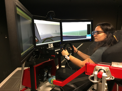
Figure 3: Autonomous driving scenario.

V-A2 Autonomous Driving

The autonomous driving study is designed to explore drivers reactions under 16 different scenarios, on a four-lane road where the participants interact with a driving simulator [3]. In each scenario, there are four potentially hazardous randomized incidents: a pedestrian crossing the road, a cyclist riding slowly in the same lane, a stopped truck in the same lane, and an oncoming truck in the other lane. The simulated car is equipped with a sensor to detect events in the roadway within 40 meters and, depending on the scenario, the car may send an auditory alarm to alert the driver. Of the 16 driving scenarios, eight are fully-autonomous. The other eight are semi-autonomous so the driver can switch between autonomous and manual driving mode. The subjects can adjust their trust level towards the system from one (lowest) to five (highest). Switching to manual driving mode will set trust level at 0. Switching from the manual to autonomous mode will set trust to three.

Traces. The study had 19 participants from [Anonymized]. Each participant had one training trial and 16 experimental trials. 9 participants were randomly selected and their driving traces (144 traces total) were used to compute the priors. Traces were captured using the PreScan software [14] which was integrated with the simulator. Each trial lasted 180 seconds resulting in a trace of 180 elements with a time step of 1 second. We recorded the vehicle dynamics, environment information, and user reactions through 32 variables.

Prior. To mimic a development context in which traces are periodically collected from the field to revisit generated invariants, each trace was analyzed once at a time and then used as a source to refine the prior estimate.

Space of invariants. Experts in the system, some of which co-authored the paper, quickly fitted 7 variables of interest into the built-in predicate patterns, expressing also the combinations that seem less promising through the constraints. For example, because the occurrence of potentially hazardous incidents was predetermined in the scenarios, those variables could be limited to the givens as no action on the part of the driver or car could trigger them. Based on the defined space, the inference tool generated 3,326 invariants.

V-B Results on Value-added for Conditional Invariants

We present the top ten invariants generated for the drone scenario in Table IV ranked in descending order by surprise ratio. (the rest of the invariants are available in the repo). Invariants are presented in the form $P(Outcome\mid Given)$. The prior probability is the probability of $Outcome$ as calculated from the prior dataset (in this study that is computed only once as we only executed the generation algorithm once). The surprise ratio shows the relation of posterior to prior, and the explanation is a straightforward description of the invariant defined formally in the first column.

Top Invariants. We start by interpreting the invariants reported in Table IV. The system developer expected P(MissionState=Complete $\mid$ MachineState=Landing, UserCommand=Default,WarningState=Default) on row 10. This is because in order for the drone to have completed its mission, it must make it back to its original starting point without incident and land. This invariant is strongly upheld by design, and so its probability will remain high across any traces supplied to the engine, especially when compared to the respective $0.05$ prior probability of $MissionState=Complete$.

TABLE IV: Drone Invariants

Invariant	Posterior	Original prior	Surprise ratio	Explanation
P(sensor.status=4 $\mid$ MissionState=PossibleTargetDetected 0.01$\leq$y-velocity$<$0.25 reaction_time=null )	0.30	0.002	159.85	When a possible target has been detected, y-velocity is low, and no user reaction has been recorded, the sensor is likely detecting a partial target.
P(UserCommand=ReturnHome $\mid$ MachineState=PossibleTargetDetected x-velocity$\geq$0.25 )	0.52	0.009	57.54	When a possible target has been detected and x-velocity is high, user has likely just issued a command to return home.
P(UserCommand=Hover $\mid$ MachineState=Sweeping x-velocity$\geq$0.25 )	0.03	0.001	49.02	When drone is performing a sweeping task and x-velocity is high, user has likely just issued a command to hover.
P(UserCommand=RequestAutoControl $\mid$ MissionState=InProgress MachineState=LosingVicon WarningState=LosingVicon )	0.28	0.01	45.93	When mission is in progress, drone has detected unreliable Vicon connectivity, and a warning has been raised for unreliable Vicon connectivity, the user has likely just issued a command to give autonomous control to the drone.
P(UserCommand=Land $\mid$ MachineState=Landing x-velocity$<$0.01 )	0.03	0.001	24.59	When machine is landing and x-velocity is low, the user has likely just issued a command to land.
P(WarningState=LosingVicon $\mid$ sensor.status=1 MachineState=LosingVicon x-velocity$<$0.01 )	0.38	0.02	20.70	When sensor has not detected any target, drone has detected unreliable Vicon connectivity, and x-velocity is low, a warning has likely been raised for unreliable Vicon connectivity.
P(reaction_time$>$7 $\mid$ MissionState=OutsideSweepArea sensor.status=3 y-velocity$\geq$0.25 )	0.23	0.01	19.85	When drone is outside the sweep area, the sensor has detected a full target, and y-velocity is high, user reaction time is likely slow.
P(MachineState=FinishedBehavior $\mid$ x-velocity$\geq$0.25 UserCommand=ReturnHome )	0.69	0.04	17.86	When x-velocity is high and user has issued a command to return home, the drone is likely finished its task.
P(MachineState=LosingVicon $\mid$ sensor.status=1 x-velocity$<$0.01 WarningState=LosingVicon )	0.47	0.03	16.85	When sensor has not detected any target, x-velocity is low, and a warning has been raised for no Vicon connectivity, the drone has likely detected loss of Vicon connectivity.
P(MissionState=Complete $\mid$ MachineState=Landing UserCommand=Default WarningState=Default )	0.76	0.05	16.72	When drone is landing, user has not issued a command, and no warning has been raised, mission is likely complete.

Some invariants had an unexpectedly high surprise ratio and were indeed surprising. Invariant P(sensor.status=4 $\mid$ MissionState=PossibleTargetDetected,0.01$\leq$y-velocity$<$0.25, reaction_time=null) with the highest surprise ratio on row 1 showed that when the drone was in a PossibleTargetDetected state and y-velocity was low, the sensor was only able to detect a partial target, perhaps indicating the need for a lower sweep speed in order to keep the full target in sensor range. The high surprise ratio of P(UserCommand=RequestAutoControl $\mid$ MissionState=InProgress, MachineState=LosingVicon, WarningState=LosingVicon ) on row 4 was unexpected because other mission states can be associated with UserCommand=RequestAutoControl, such as use of manual control to return to Vicon connectivity, which can occur during any machine state. This invariant tells us that the user had difficulty perceiving when localization connectivity was re-established and tried using autonomous control when it was not possible, which could be an opportunity for system improvement. P(reaction$\_$time$>$7 $\mid$ MissionState=OutsideSweepArea, sensor.status=3, y-velocity$\geq$0.25 ) on row 7 was also unexpectedly high. The predicate reaction$\_$time$>$7 can be associated with any command, but it seems to be most closely associated with end-of-mission commands as it is most closely related to MissionState=OutsideSweepArea. The slow reaction time when the sensor is detecting a full target and the drone is outside the sweep area could indicate a need for sensor stabilization or a higher x-velocity at that time.

Priors Comparison. When we compare the common predicates between invariants in Table IV and priors in Table V, we also find marked dissimilarities. For example, predicates $flight\_data.battery\_low$, $y\mathchar 45\relax velocity<0.01$, and $0.01\leq x\mathchar 45\relax velocity<0.25$ do not appear in the top ten conditional invariants. Out of the 25 total unique predicates in Table IV only 5 also appear in the top ten priors. This shows that stateful conditioning has a significant impact upon the probability of predicates.

Daikon Comparison. We then compare our approach to the perennially popular inference engine Daikon, primarily aiming to highlight the differences and the potential complementary nature of the approaches. Table VI shows the output for a tweaked version of Daikon that includes the invariant probabilities for single-predicate splitting and allows for expression of stateful behavior as a conjunction. The probabilities of the UserCommand predicates in Table VI and Table IV, show that the Daikon invariants capture probabilities closer to unconditioned prior probabilities, but give no indication of the circumstances under which those commands occur. In the warning$\_$state$\_$change entry point, we see that the range of x-velocities is similar to the Bayesian invariant P(WarningState=LosingVicon $\mid$ sensor.status=1, MachineState=LosingVicon, x-velocity$<$0.01) on row 6. However, this is not a conditional invariant but rather a conjunction of sensor.status==1 $\land$ x-velocity $\geq$ -0.609 which holds with confidence $\geq$0.95 at this program point. Moreover, it is not possible to split this program point using more than one predicate at a time, thus overlooking most of the invariants in Table IV. While these invariants are informative, they do not provide the conditional probabilities of our approach. Yet, Daikon provides a much richer set of builtin predicates than the ones covered by our implementation so we see much potential in their integration.

Overall, the generated conditional probabilistic invariants confirm defined-by-design properties and expose properties of the drone ISR system that were heretofore unknown or not obvious and not captured by existing approaches.

TABLE V: Top Prior probabilities for Drone.

Predicate	Prior
UserCommand=Default	0.958
flight$\_$data.battery$\_$low=False	0.950
WarningState=Default	0.897
status.data=1	0.724
MachineState=Sweeping	0.427
y-velocity $<$ 0.01	0.426
MissionState=InsideSweepArea	0.405
0.01 $\leq$ x-velocity $<$ 0.25	0.390
x-velocity $<$ 0.01	0.376
0.01 $\leq$ y-velocity $<$ 0.25	0.354

TABLE VI: Daikon Drone Invariants

Daikon Drone Invariants
/flight_data.battery_low one of { “False” (90.83%), “True” (9.17%) }
MissionState one of { “Complete” (4.63%), “InProgress” (9.14%), “InsideSweepArea” (37.34%), “OutsideSweepArea” (22.76%), “PossibleTargetDetected” (18.21%), “Suspended”(7.21%), “AbortingMission” (0.73%) }
UserCommand one of { “None” (1.00%), ”Hover” (0.55%), “KeepSweeping” (2.51%), “Land” (0.73%), “LookCloser” (58.75%), “RequestAutoControl” (11.79%), “RequestManualControl” (13.85%), “ReturnHome” (10.83%)}
reaction_time $\geq$ 0.0
..warning_state_change():::ENTER;condition=“sensor.status == 1” y-velocity $\leq$ 0.23 x-velocity $\geq$ -0.61

V-C Results on Value-added with Data Updates

Similar to the drone scenario, some of the initially generated invariants with the highest posterior likelihood confirm our understanding of how the autonomous vehicle operates while others render interesting surprises. For example, the invariant P(TrustChange$<$0 $\mid$
Brake==0 Mode=autonomous
Throttle$>$0 Event=None WheelChange$\geq$20 ) says that, when the brake is not engaged, mode is autonomous, throttle is engaged, nothing is detected in the roadway, and wheel angle is changing quickly, a decrease in trust is likely to occur. This may indicate that the controller for the car’s angular motion makes drivers uncomfortable. Also similar are the noticeable differences between conditioned and non-conditioned probabilities as shown by the differences between posteriors and priors. For example, of the outcome predicates, $TrustChange>0$, $TrustChange==0$, and $Brake>0$ do not appear in the priors. Of the givens, $Throttle==0$, $TrustChange>0$, and all $Event$ predicates excepting $Event=None$ do not appear in the priors.

However, in this question, we want to focus on the exploration of the effects of processing new traces and update priors in the generation and refinement of computed invariants. To do that, we assume that the traces generated by each participant driving the autonomous vehicle are sequentially received and processed by the inference generation engine. So new traces are used to refine or create invariants as well as to update priors for the next trace. Figure 4 plots, for the 19 set of traces (invariant generation iterations in the x-axis), the variance of the surprise ratio of the generated invariants. A decrease in variance indicates that the surprise ratio of that particular invariant is converging, suggesting that the prior and posterior have both converged as well. From there, model selection was used according to a modified Bayesian Information Criterion to constrain resulting invariants to low-entropy models. This was in order to determine whether the resulting distributions of prior and posterior were beginning to converge, hopefully affording some guarantee of predictability in future traces.

Figure 4 shows some invariants with marked peaks, indicating a large surprise potentially due to an aberrant trace, while some have low variance throughout, meaning that the posterior and prior do not change greatly between iterations.

In the autonomous driving scenario, alarms are important to get drivers’ attention and alert them to possible incidents. Invariant P(Brake$>$0 $\mid$ Mode=autonomous Event=pedestrian detected WheelChange$\geq$20 TrustChange$<$0 ), the topmost light blue line in the graph, shows a high degree of surprise variance early on in trace collection. This is mostly due to the fact that the initial prior is uniform, and in actuality pedestrians are an uncommon occurrence with a probability of $0.03$. This is the unconditioned probability by system design, and though there are three early traces in which this invariant occurs, the addition of more traces allows the prior to converge and thus the variance drops.

Trust affects human drivers’ reliance on the system. P(Trust$<$0 $\mid$ Speed$>$0 Mode=autonomous Event=obstacle detected ) indicated by the purple line second closest to the x-axis, tells that when an obstacle is in the roadway, the car is under autonomous control, and the speed is nonzero, the trust level is more likely to decrease. The fact that the user must manually decrease the trust, either by self-reporting or by taking the car to manual mode, seems to indicate this is a perceived safety issue on the part of the human in the loop. Fully understanding the trust evolution contributes to a trustworthy system.

As with the previous drone study, the invariants generated for the autonomous vehicle confirmed expected known design attributes and helped to identify overlooked properties that characterize the system in the deployed situation. Particularly relevant to this portion of the study, however, is how new information can be easily processed by the engine to generate new invariants, taking into consideration either new traces or updated prior distributions. It is also worth noticing how, at any given point in time, the surprise ratio is able to highlight different invariants as either the trace captures some new behavior or the prior changes, bringing to attention different aspects learned from the system.

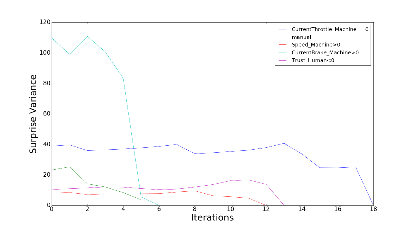
Figure 4: Variance of surprise ratio per iteration for driving scenario probabilistic invariants that exhibit high variance of surprise ratio.

VI CONCLUSIONS

In this work we have introduced what may be the first automated approach to generate conditional probabilistic invariants leveraging Bayesian inference. Our study showed its viability and potential in two distinct autonomous systems/contexts. While most invariant use cases apply to probabilistic conditional invariants, we believe that a probabilistic understanding of stateful behavior can quantitatively reaffirm properties, assist in the discovery of unexpected behaviors appearing only under certain contexts, and expose potential opportunities to optimize a system with greater context specificity.

VII APPENDIX

In this Appendix with provide additional study data and explanations that we could not fit in the paper submission.

TABLE VII: Driving Invariants

Invariant	Posterior	Original prior	Surprise Ratio	Explanation
P(Brake$>$0 $\mid$ Mode=autonomous Throttle==0 Event=pedestrian detected TrustChange$>$0 )	0.97	0.04	21.85	When mode is autonomous, throttle is not engaged, a pedestrian is in the roadway, and trust has increased, brake is likely engaged.
P(Throttle==0 $\mid$ Mode=autonomous Event=pedestrian detected )	1	0.1	10.26	When mode is autonomous and a pedestrian is in the roadway, throttle is likely not engaged.
P(Mode=manual $\mid$ Throttle==0 Event=None )	0.95	0.15	6.40	When throttle is not engaged and nothing is detected in the roadway, mode is likely manual.
P(WheelChange$<$20 $\mid$ Mode=autonomous Event=None )	0.53	0.50	2.91	When mode is autonomous and nothing is detected in the roadway, wheel angle is likely changing slowly.
P(TrustChange$>$0 $\mid$ Brake==0 Mode=manual Throttle$>$0 Event=None )	0.31	0.12	2.695	When brake is not engaged, mode is manual, throttle is engaged, and nothing is detected in the roadway, trust is likely increasing.
P(WheelChange$>=$20 $\mid$ Brake==0 Mode=autonomous Throttle$>$0 Event=cyclist detected TrustChange¡0 )	0.90	0.5	1.79	When brake is not engaged, mode is autonomous, throttle is engaged, a cyclist is in the roadway, and trust increased, wheel angle is likely changing quickly.
P(TrustChange$<$0 $\mid$ Brake==0 Mode=autonomous Throttle$>$0 Event=None WheelChange$>=$20 )	0.15	0.12	1.21	When brake is not engaged, mode is autonomous, throttle is engaged, nothing is detected in the roadway, and wheel angle is changing quickly, trust is likely to decrease.
P(Throttle$>$0 $\mid$ Mode=autonomous Event=None )	1	0.90	1.11	When mode is autonomous and nothing is detected in the roadway, throttle is likely engaged.
P(Brake==0 $\mid$ Mode=autonomous Event=None )	1	0.96	1.05	When mode is autonomous and nothing is detected in the roadway, brake is likely not engaged.
P(TrustChange==0 $\mid$ Brake==0 Mode=autonomous Throttle¿0 Event=None WheelChange$>=$20 )	0.77	0.77	1.01	When brake is not engaged, mode is autonomous, throttle is engaged, nothing has been detected in the roadway, and wheel angle is changing quickly, trust is likely to remain constant.

VIII Autonomous Vehicle Invariants

This analysis is relevant to the second study in the paper.

Table VII includes the top 10 invariants generated for the autonomous vehicle. We briefly comment on them here.

Invariant P(Brake$>$0 — Mode=autonomous Throttle==0 Event=pedestrian detected TrustChange$>$0 ) on row 1 had the highest surprise ratio, possibly due to the specific behavior the autonomous controller exhibited in the presence of a pedestrian and the trust-building effect it had on the human in the loop.

Invariant P(Throttle==0 $\mid$ Mode = autonomous Event=pedestrian detected ) on row 2 had a similarly high surprise ratio, with posterior likelihood of 1.0 indicating that when the car is autonomously controlled and a pedestrian is in the roadway, the throttle is no longer engaged.

This has a slightly higher probability than P(Brake$>$0 $\mid$ Mode=autonomous Throttle==0 Event=pedestrian detected TrustChange $>$0 ), likely because the throttle must be disengaged before brake can be engaged, and the brake may be engaged for multiple reasons, such as a different event or a curve in the road. The inclusion of predicate $TrustChange>0$ in the givens was surprising as well, as it indicates that an increase in trust in conjunction with detecting a pedestrian is correlated with a subsequent application of the brakes. Note that this is not a causal relationship, as the autonomous driving algorithm does not react to changes in trust from the human in the loop.

Dealing with incidents on the road is essential to demonstrate realistic safety behaviors in the autonomous driving scenario. Invariants given Event=Pedestrian detected characterize the performance of the simulated car when handling the incident of pedestrian crossing the road. The car decreases the velocity by applying brake and easing the throttle, but no wheel change is closely associated according to the model selection algorithm. It fits the expectation that the car tends to slow down, rather than changing lanes to bypass the pedestrian. In larger models, both $WheelChange>=20$ and $WheelChange<20$ predicates present with no significant change to the posterior likelihood, showing that the posterior likelihood is more strongly conditioned on a change in $Throttle$.

On the other hand, invariants given Event=Cyclist detected shows that the car performs a steep turn and unexpectedly accelerates in order to avoid the cyclist. Outside of the top ten, similar invariants can be found involving $Event=Truck$, which shows that the car again unexpectedly accelerates when passing the incoming truck on the other lane. These invariants present trends that the designers were unaware of and provide direct guidance on improving the system design when handling incidents.

In the autonomous driving scenario, alarms are important to alert drivers and get their attention to possible incidents. We intentionally injected false alarms to test the car’s performance. The expected invariant $P(-20<=WheelChange<=20\mid Event=FalseAlarm)$ tells that the car maintains slight change of the wheel, while the unexpected invariant $P(VelocityChange<0\mid Event=FalseAlarm)$ indicates a velocity decrease. Recall that false alarm is an auditory alarm when there is no real incident on the road. Even though the false alarm does not cause the car to react too much on the wheel, it causes the car to slow down to check if there is any incident. False alarms improve the safety of the system by detecting potential hazards more conservatively, though too many false alarms may lead to driver’s alarm fatigue.

Invariants related to $Mode$ provide the information during manual driving or autonomous driving. Invariant P(TrustChange$>$0 $\mid$ Brake==0 Mode=manual Throttle$>$0 Event=None ) on row 5 shows that human drivers tend to increase their trust following “normal” operation in manual mode. This also indicates that they subsequently leave manual mode, as it is not possible to raise trust in manual mode.

$P(Mode=Manual\mid Throttle=0)$ with a ratio of 3.986 and $P(Mode=Autonomous\mid Throttle=0)$ with a ratio of 0.481 tells that given throttle is not used, the car is more likely to be in manual driving mode. These invariants shows that human drivers tends to be unsatisfied by the speed of the autonomous driving and they are confident of driving manually. This can help the designer of the system to understand human driver’s behavior and adjust the performance of the system.

Trust affects human drivers’ reliance on the system. P(TrustChange $<$ 0 $\mid$ Brake==0 Mode=autonomous Throttle$>$0 Event=None WheelChange $>=$ 20 ) on row 7 tells that when throttle is engaged and the wheel angle is changing quickly, the trust level is more likely to decrease. The absence of an $Event$ seems to indicate this is a perceived safety issue on the part of the human in the loop.

However, P(TrustChange==0 $\mid$ Brake==0 Mode=autonomous Throttle$>$0 Event=None WheelChange $>=$ 20 ) on row 10 shows us that the human in the loop is more likely to leave trust unchanged under those same conditions. This seems to indicate that there are latent variables not being accounted for, possibly in the system or on the part of the user. Fully understanding the trust evolution contributes to a trustworthy system.

IX Preliminary Results on Inference Computation Cost

We explore What is the cost of generating conditional invariants?. We assess cost in terms of the time to generate the invariants as a function of the number of predicates and trace length.

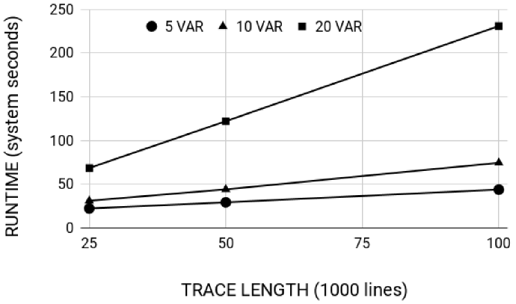
Figure 5: Runtime vs. trace length and number of predicates.

We briefly assess the dimensions of the space of invariants to explore and the associated inference cost. Figure 5 plots the runtime cost in system seconds when executing the inference engine on traces of three different lengths (25K, 50K, 100K) produced by the Drone ISR when three different sets of predicates are explored (5, 10 and 20 variables of $Range$ type with two predicates each). Runtime tests were performed on a containerized Linux box with an x86$\_$64 AMD FX-8120E 3.1GHz 8-core processor.

As the graph shows, the runtime of the engine depends on both trace length and predicate complexity, but the influence of the number of variables seems to dominate the space to explore as it grows exponentially when the variables are considered as both outcomes and givens. As the number of variables grows, a developer can control this cost through the specification of the predicate space provided to the engine by specifying whether a variable is to be explored as a given or as an outcome, or more restrictively by aiming for particular pairs of variable predicates.

References

- [1] Maryam Raiyat Aliabadi, Amita Ajith Kamath, Julien Gascon-Samson, and Karthik Pattabiraman. Artinali: Dynamic invariant detection for cyber-physical system security. In Proceedings of the 2017 11th Joint Meeting on Foundations of Software Engineering, ESEC/FSE 2017, page 349–361, New York, NY, USA, 2017. Association for Computing Machinery.
- [2] Glenn Ammons, Rastislav Bodı k, and James R. Larus. Mining specifications. In Proceedings of the 29th ACM SIGPLAN-SIGACT Symposium on Principles of Programming Languages, POPL ’02, pages 4–16, New York, NY, USA, 2002. ACM.
- [3] Force Dynamics. Force dynamics cr 401. https://www.force-dynamics.com/, 2019.
- [4] M. D. Ernst, J. H. Perkins, P. J. Guo, S. McCamant, C. Pacheco, M. S. Tschantz, and C. Xiao. The daikon system for dynamic detection of likely invariants. In Science of Computer Programming, volume 69, pages 35–45, 2007.
- [5] Michael D. Ernst, Adam Czeisler, William G. Griswold, and David Notkin. Quickly detecting relevant program invariants. In ICSE, 2000.
- [6] C. Scott Ananian et. al. Cup parser generator for java. https://www.cs.princeton.edu/~appel/modern/java/CUP/, 2015.
- [7] Apache Software Foundation. Commons math: The apache commons mathematics library. https://commons.apache.org/proper/commons-math/index.html, August 2016.
- [8] Apache Software Foundation. Commons lang. https://commons.apache.org/proper/commons-lang/, April 2019.
- [9] Open Source Robotics Foundation. rosbag package summary. http://wiki.ros.org/rosbag, 2015.
- [10] Open Source Robotics Foundation. Robot operating system. https://www.ros.org/, 2019.
- [11] Mark Gabel and Zhendong Su. Javert: fully automatic mining of general temporal properties from dynamic traces. In SIGSOFT FSE, 2008.
- [12] L. Grunske. Specification patterns for probabilistic quality properties. In 2008 ACM/IEEE 30th International Conference on Software Engineering, pages 31–40, May 2008.
- [13] Sudheendra Hangal and Monica S. Lam. Tracking down software bugs using automatic anomaly detection. In Proceedings of the 24th International Conference on Software Engineering, ICSE ’02, pages 291–301, New York, NY, USA, 2002. ACM.
- [14] TASS International. Prescan overview. https://tass.plm.automation.siemens.com/prescan-overview, 2019.
- [15] L. Itti and P. F. Baldi. Bayesian surprise attracts human attention. In Advances in Neural Information Processing Systems, Vol. 19 (NIPS*2005), pages 547–554, Cambridge, MA, 2006. MIT Press.
- [16] Hengle Jiang, Sebastian G. Elbaum, and Carrick Detweiler. Reducing failure rates of robotic systems though inferred invariants monitoring. In 2013 IEEE/RSJ International Conference on Intelligent Robots and Systems, Tokyo, Japan, November 3-7, 2013, pages 1899–1906, 2013.
- [17] Hengle Jiang, Sebastian G. Elbaum, and Carrick Detweiler. Inferring and monitoring invariants in robotic systems. Auton. Robots, 41(4):1027–1046, 2017.
- [18] Tien-Duy B. Le and David Lo. Deep specification mining. In ISSTA, 2018.
- [19] Davide Lorenzoli, Leonardo Mariani, and Mauro Pezzè. Automatic generation of software behavioral models. 2008 ACM /IEEE 30th International Conference on Software Engineering, pages 501–510, 2008.
- [20] ThanhVu Nguyen, Matthew B. Dwyer, and Willem Visser. Symlnfer: Inferring program invariants using symbolic states. 2017 32nd IEEE /ACM International Conference on Automated Software Engineering (ASE), pages 804–814, 2017.
- [21] Thanhvu Nguyen, Deepak Kapur, Westley Weimer, and Stephanie Forrest. Dig: A dynamic invariant generator for polynomial and array invariants. ACM Trans. Softw. Eng. Methodol., 23(4):30:1–30:30, September 2014.
- [22] Martin P. Robillard, Eric Bodden, David Kawrykow, Mira Mezini, and Tristan Ratchford. Automated api property inference techniques. IEEE Transactions on Software Engineering, 39:613–637, 2013.
- [23] Ryze Robotics. Tello user manual v1.0. https://dl-cdn.ryzerobotics.com/downloads/Tello/20180212/Tello+User+Manual+v1.0_EN_2.12.pdf, 2018.
- [24] Vicon Motion Systems. Vicon motion capture. https://www.vicon.com/motion-capture/, 2019.
- [25] Neil Walkinshaw, Ramsay Taylor, and John Derrick. Inferring extended finite state machine models from software executions. Empirical Software Engineering, 21(3):811–853, Jun 2016.
- [26] Ernst Wit, Edwin van den Heuvel, and Jan-Willem Romeijn. ‘All models are wrong…’: an introduction to model uncertainty. Statistica Neerlandica, 66(3):217–236, August 2012.
- [27] Jinlin Yang, David Evans, Deepali Bhardwaj, Thirumalesh Bhat, and Manuvir Das. Perracotta: Mining temporal api rules from imperfect traces. In Proceedings of the 28th International Conference on Software Engineering, ICSE ’06, pages 282–291, 2006.