Hairi, Liu, and Ying

Calculable Error Bounds of the Power-of-Two-Choices in Heavy-Traffic

Beyond Scaling: Calculable Error Bounds of the Power-of-Two-Choices Mean-Field Model in Heavy-Traffic

Hairi Electrical, Computer and Energy Department, Arizona State University, Tempe, AZ 85281, fhairi@asu.edu Xin Liu and Lei Ying Electrical Engineering and Computer Science Department, University of Michigan, Ann Arbor, MI 48109, xinliuee@umich.edu, leiying@umich.edu

This paper provides a recipe for deriving calculable approximation errors of mean-field models in heavy-traffic with the focus on the well-known load balancing algorithm — power-of-two-choices (Po2). The recipe combines Stein’s method for linearized mean-field models and State Space Concentration (SSC) based on geometric tail bounds. In particular, we divide the state space into two regions, a neighborhood near the mean-field equilibrium and the complement of that. We first use a tail bound to show that the steady-state probability being outside the neighborhood is small. Then, we use a linearized mean-field model and Stein’s method to characterize the generator difference, which provides the dominant term of the approximation error. From the dominant term, we are able to obtain an asymptotically-tight bound and a nonasymptotic upper bound, both are calculable bounds, not order-wise scaling results like most results in the literature. Finally, we compared the theoretical bounds with numerical evaluations to show the effectiveness of our results. We note that the simulation results show that both bounds are valid even for small size systems such as a system with only ten servers.

Mean-field model, power-of-two-choices, heavy-traffic analysis, Stein’s method, state-space-concentration

1 Introduction

Large-scale and complex stochastic systems have become ubiquitous, including large-scale data centers, the Internet of Things, and city-wide ride-hailing systems. Queueing theory has been a fundamental mathematical tool to model large-scale stochastic systems, and to analyze their steady-state performance. For example, steady-state analysis of load balancing algorithms in many-server systems is one of the most fundamental and widely-studied problems in queueing theory Harchol-Balter (2013). When the stationary (steady-state) distribution is known, the mean queue length and waiting time can be easily calculated, which reveal the performance of the system and can be used to guide the design of load balancing algorithms. However, for large-scale stochastic systems in general, it is extremely challenging (if not impossible) to characterize a system’s stationary distribution due to the curse of dimensionality. For example, in a queueing system with $N$ servers, each with a buffer of size $b,$ the size of state space is at the order of $N^{b}$. Moreover, in such a system, the transition rate from a state to another may be state-dependent, so it becomes almost impossible to characterize its stationary distribution unless the system has some special properties such as when the stationary distribution has a product form Srikant and Ying (2014). To address these challenges, approximation methods such as mean-field models, fluid models, or diffusion models have been developed to study the stationary distributions of large-scale stochastic systems.

This paper focuses on stochastic systems with many agents, in particular, a many-server, many-queue system such as a large-scale data center. For such systems, mean-field models have been successfully used to approximate the stationary distribution of the system in the large-system limit (when the system size becomes infinity), see e.g. the seminal papers on power-of-two-choices Mitzenmacher (1996), Vvedenskaya et al. (1996). These earlier results, however, are asymptotic in nature by showing that the stationary distribution of the stochastic system weakly converges to the equilibrium point of the corresponding mean-field model as the system size becomes infinity. So these results do not provide the rate of convergence or the approximation error for finite-size stochastic systems. Furthermore, because the asymptotic nature of the traditional mean-field model, it only applies to the light-traffic regime where the normalized load (load per server) is strictly less than the per-server capacity in the limit.

Both issues have been recently addressed using Stein’s method. Ying (2016) studied the approximation error of the mean-field models in the light-traffic regime using Stein’s method, and showed that for a large-class of mean-field models, the mean-square error is $O\left(\frac{1}{N}\right),$ where $N$ is the number of agents in the system. Ying (2017) further extended Stein’s method to mean-field models for heavy-traffic systems and developed a framework for quantifying the approximation errors by connecting them to the local and global convergence of the mean-field models. While these results overcome the weakness of the traditional mean-field analysis, they only provide order-wise results, i.e. the scaling of the approximation errors in terms of the system size. Later, a refined mean-field analysis was developed in Gast (2017), Gast and Van Houdt (2018). In particular, Gast and Van Houdt (2018) established the coefficient of the $\frac{1}{N}$ approximation error for light-traffic mean-field models, which provides an asymptotically exact characterization of the approximation error. However, the refined result in Gast and Van Houdt (2018) is based on the light-traffic mean-field model and the analysis uses a limiting approach. Therefore, the result and method do not apply to heavy-traffic mean-field models.

This paper obtains calculable error bounds of heavy-traffic mean-field models. We consider the supermarket model Mitzenmacher (1996), and assume jobs are allocated to servers according to a load balancing algorithm called power-of-two-choices Mitzenmacher (1996), Vvedenskaya et al. (1996). While the approximation error of this system has been studied in Ying (2017), it only characterizes the order of the error (in terms of the number of servers) and does not provide a calculable error bound. The difficulty is that the mean-field model of power-of-two-choices is a nonlinear system, so quantifying the convergence rate explicitly is difficult. In this paper, we overcome this difficulty by focusing on a linearized heavy-traffic mean-field model, linearized around its equilibirium point, so that we can explicitly solve Stein’s equation. The linearized model cannot approximate the system well when the state of the system is not near equilibrium, which is taken care of by using a geometric tail bound to show that such deviation only occurs with a small probability.

This paper is an extended version of our conference paper Hairi et al. (2021). This paper includes the details of the state-space-concentration (SSC) result and the bound on the entries of the inverse of the Jacobian matrix, both were omitted in Hairi et al. (2021) due to the page limit. We also include an order-wise error bound which can be applied to a larger range of $\alpha$ than that in Ying (2017). This result was not included in Hairi et al. (2021). The main results of this paper are summarized below.

• For the supermarket model with power-of-two-choices, we obtain two error bounds for the system in heavy-traffic. We first characterize the dominating term in the approximation error, which is a function of the Jacobian matrix of the mean-field model at its equilibrium and is asymptotically accurate, and then obtain a general upper bound which holds for finite size systems. We obtain the explicit forms of both bounds so they are calculable given the load and the system size. Also, we obtained an order-wise error bound in terms of size size $N$ and heavy-traffic parameter $\alpha$.

• From the methodology perspective, the combination of state-space-concentration (SSC) and the linearized mean-field model provides a recipe for studying other mean-field models in heavy-traffic. The most difficult part of applying Stein’s method for mean-field models is to establish the derivative bounds. While perturbation theory Khalil (2001) provides a principled approach, we can only obtain order-wise results when facing nonlinear mean-field models (see e.g. Ying (2017)). Our approach is based on a basic hypothesis that if the mean-field solution would well approximate the steady-state of the stochastic system, then the steady-state should concentrate around the equilibrium point. Therefore, the focus should be on the mean-field system around its equilibrium point, which can be reduced to a linearized version. This basic hypothesis can be supported analytically using SSC based on the geometric tail bound Bertsimas et al. (2001). In other words, the state-space-concentration result leads to a linear system with a “solvable” Stein’s equation, which is the key for applying Stein’s method for steady-state approximation.

2 Related Work

This section summarizes the related results in two categories. From the methodology perspective, this paper follows the line of research on using Stein’s method for steady-state approximation of queueing systems introduced in Braverman et al. (2016), Braverman and Dai (2017). This paper uses Stein’s method for mean-field approximations, which has been introduced in Ying (2016) and extended in Ying (2017), Liu and Ying (2018), Gast (2017), Gast and Van Houdt (2018). Stein’s method for mean-field models (or fluid models) can also be interpreted as drift analysis based on integral Lyapunov functions, which was introduced in an earlier paper Stolyar (2015). The combination of SSC and Stein’s method was used in Braverman and Dai (2017), which introduces Stein’s method for steady-state diffusion approximation of queueing systems. The framework is later applied to mean-field (fluid) models where Stein’s equation for a simplified one-dimensional mean-field models can be solved Liu and Ying (2019, 2020). In this paper, the linearized system is still a multi-dimensional system. SSC has been used in heavy-traffic analysis based on the Lyapunov-drift method, which was developed in Eryilmaz and Srikant (2012) and used for analyzing computer systems and communication systems (see e.g. Maguluri and Srikant (2016), Wang et al. (2018)).

From the perspective of the power-of-two-choices load-balancing algorithm, for the light-traffic regime, Vvedenskaya et al. (1996) proved the weak convergence of the stationary distribution of power-of-two-choices to its mean field limit in the light traffic regime, the order-wise rate of convergence was established in Ying (2016), and Gast and Van Houdt (2018) proposed a refined mean-field model with significantly smaller approximation errors. The scaling of queue lengths of power-of-two-choices in heavy-traffic has only recently studied, first in Eschenfeldt and Gamarnik (2016) for finite-time analysis (transient analysis) and then in Ying (2017) for steady-state analysis. Our result was inspired by Gast and Van Houdt (2018), which refines the mean-field model using the Jacobian matrix of the light-traffic mean-field equilibrium. Different from Gast and Van Houdt (2018), based on state-space-concentration and linearized mean-field model, we established calculable error bounds for heavy-traffic mean-field models where the mean-field equilibrium and the associated Jacobian matrix are both functions of the system load and system size, which prevented us from using the asymptotic approach used in Gast and Van Houdt (2018).

3 System Model

In this section, we first introduce the well-known supermarket model under the power-of-two-choices load balancing algorithm. Our focus is the stationary distribution of such a system in the heavy-traffic regime (i.e. the load approaches to one as the number of servers increases).

Then, we present the mean-field model, tailored for the $N$-server system Ying (2017) and the exact load of the $N$-server system. The solution of the mean-field model is an approximation of the stationary distribution of the stochastic system. We will then present the approach to characterize the approximation error based on Stein’s equation.

Consider a many-server system with $N$ homogeneous servers, where job arrivals follow a Poisson process with rate $\lambda N$ and service times are i.i.d. exponential random variables with rate one. Each server can hold at most $b$ jobs, including the one in service. We consider $\lambda=1-\frac{\gamma}{N^{\alpha}}$ for some $0<\gamma\leq 1$ and $\alpha\geq 0$. When $\alpha=0$, $\lambda$ is a constant independent of $N$ which we call the light-traffic regime. When $\alpha>0$, the arrival rate depends on $N$ and approaches to one as $N\rightarrow\infty,$ which we call the heavy-traffic regime. We assume the system is under a load balancing algorithm called power-of-two-choices Mitzenmacher (1996), Vvedenskaya et al. (1996).

Power-of-Two-Choices (Po2): Po2 samples two servers uniformly at random among $N$ servers and dispatches the incoming job to the server with the shorter queue size. Ties are broken uniformly at random.

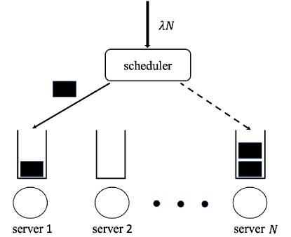
Figure 1: Power-of-Two-Choices

Let $S_{i}(t)$ denote the fraction of servers with queue size at least $i$ at time $t.$ The term $S_{0}(t)=1,\forall t$ by definition. Under the finite buffer assumption with buffer size $b$, $S_{i}(t)=0,\forall i\geq b+1,\forall t.$ Throughout the paper, we assume that the buffer size b can be up to the order of $\log N$, i.e. $b=O(\log N)$. Define $\mathcal{S}$ to be

$$\mathcal{S}=\{s~{}|~{}1\geq s_{1}\geq\cdots\geq s_{b}\geq 0\},$$

and $S(t)=[S_{1}(t),S_{2}(t),\cdots,S_{b}(t)]$. It is easy to verify that the state $S(t)$ is a continuous time Markov chain (CTMC). Define $e_{k}$ to be a $b$-dimensional vector such that the $k$th entry is one and all other entries are zero. We characterize the transition rates $R_{s,s^{\prime}}$ from $s$ and $s^{\prime}$ as follows:

$$R_{s,s^{\prime}}=\\ \begin{cases}N(s_{k}-s_{k+1}),\text{if }s^{\prime}=s-\frac{e_{k}}{N}\text{ and }1\leq k\leq b-1\\ Ns_{b},\text{if }s^{\prime}=s-\frac{e_{b}}{N}\\ \lambda N(s^{2}_{k-1}-s^{2}_{k}),\text{if }s^{\prime}=s+\frac{e_{k}}{N}\\ \sum_{k=1}^{b}-\lambda N(s^{2}_{k-1}-s^{2}_{k})-N(s_{k}-s_{k+1}),\text{if }s^{\prime}=s\\ 0,\text{otherwise}\end{cases}$$

The first and second terms correspond to the event that a job departs from a server with queue size $k$ so $s_{k}$ decreases by $\frac{1}{N},$ and the third term corresponds to the event that a job arrives and joins a server with queue size $k-1.$ We define a normalized transition rate to be

$$q_{s,s^{\prime}}=\frac{R_{s,s^{\prime}}}{N}.$$

We focus on the steady-state analysis of the system, i.e. the distribution of $S(\infty)$. At the steady-state, $S(\infty)$ is a $b$-dimensional random vector. For simplicity, we let $S$ denote $S(\infty)$. In this paper, we use uppercase letters for random variables and lowercase letters for deterministic values.

The mean-field model Mitzenmacher (1996), Vvedenskaya et al. (1996), Ying (2017) for this system is

$$\dot{s}=f(s)=\sum_{s^{\prime}:s^{\prime}\neq s}R_{s,s^{\prime}}(s^{\prime}-s)=N\sum_{s^{\prime}:s^{\prime}\neq s}q_{s,s^{\prime}}(s^{\prime}-s).$$

According to the definition of $R_{s,s^{\prime}}$ and $q_{s,s^{\prime}},$ we have

$$\dot{s}_{k}=f_{k}(s)=\begin{cases}\lambda(s^{2}_{k-1}-s^{2}_{k})-(s_{k}-s_{k+1}),&1\leq k\leq b-1\\ \lambda(s^{2}_{b-1}-s^{2}_{b})-s_{b},&k=b.\end{cases}$$

The equilibrium point of this mean-field model, denoted by $s^{*},$ satisfies the following conditions:

$$s^{*}_{0} =1$$ (1a)

$$\lambda\left((s^{*}_{k-1})^{2}-(s^{*}_{k})^{2}\right)-(s^{*}_{k}-s^{*}_{k+1}) =0,\quad 1\leq k\leq b-1$$ (1b)

$$\lambda\left((s^{*}_{b-1})^{2}-(s^{*}_{b})^{2}\right)-s^{*}_{b} =0.$$ (1c)

The existence and uniqueness of the equilibrium point has been proved in Mitzenmacher (1996). Define

$$g(s)=-\int_{0}^{\infty}d(s(t),s^{*})dt,\quad s(0)=s.$$

where $d(s(t),s^{*})$ is a distance function. Then, by the definition of $g(s),$ we have

$$\nabla g(s)\cdot f(s)=d(s,s^{*}).$$ (2)

Equation (2) is called the Poisson equation or Stein’s equation. For any bounded $g,$ we have the following steady state equation (Basic Adjoint Relationship (BAR) Glynn and Zeevi (2008))

$$\mathbb{E}[Gg(S)]=0,$$ (3)

where the expectation is taken with respect to the steady state distribution of $S$ and $G$ is the generator of the CTMC. Combining (2) and (3), we have

$$\mathbb{E}\left[d(S,s^{*})\right]= \mathbb{E}\left[\nabla g(S)\cdot f(S)-Gg(S)\right]$$

$$= -\mathbb{E}\left[\sum_{s^{\prime}}R_{S,s^{\prime}}\Gamma(S,s^{\prime})\right],$$ (4)

where $\Gamma(s,s^{\prime})=g(s^{\prime})-g(s)-\nabla g(s)\cdot(s^{\prime}-s)$. From (4), Stein’s method provides us a way to study the approximation error defined by $\mathbb{E}[d(S,s^{*})]$ by bounding the generator difference between the original system and the mean-field model.

4 Main Results and Methodology

This section summarizes our main results, which include an asymptotically tight approximation error bound and an upper bound that holds for finite $N.$ We remark again the bounds in Theorem 4.1 and Corollary 4.2 can be calculated numerically and are not order-wise results as in most earlier papers.

Theorem 4.1 (Asymptotically Tight Bound)

For $0<\alpha<\frac{1}{18}$, we have that

$$\mathbb{E}[||S-s^{*}||^{2}]=-\frac{1}{N}\sum_{i=1}^{b}[J^{T}(s^{*})]^{-1}_{ii}\tilde{f}_{i}(s^{*})+o\left(\frac{1}{N^{1+\alpha}}\right)$$ (5)

where

$$J(s^{*})=\left[\begin{matrix}-2\lambda s^{*}_{1}-1&1&&0\\ 2\lambda s^{*}_{1}&\ddots&\ddots&\\ &\ddots&\ddots&1\\ 0&&2\lambda s^{*}_{b-1}&-2\lambda s^{*}_{b}-1\end{matrix}\right]$$

is the Jacobian matrix of the mean-field model $f(s)$ at equilibrium point $s^{*},$ and

$$\tilde{f}_{i}(s^{*})=\frac{1}{2}[\lambda\left((s^{*}_{i-1})^{2}-(s^{*}_{i})^{2}\right)+(s^{*}_{i}-s^{*}_{i+1})]$$

for $i=1,2,\cdots,b$.

The theorem states that the mean square error $\mathbb{E}[||S-s^{*}||^{2}]$ has an asymptotic dominating term

$$-\frac{1}{N}\sum_{i=1}^{b}[J^{T}(s^{*})]^{-1}_{ii}\tilde{f}_{i}(s^{*}).$$

Therefore, we have

$$\lim_{N\rightarrow\infty}N\mathbb{E}[||S-s^{*}||^{2}]=-\sum_{i=1}^{b}[J^{T}(s^{*})]^{-1}_{ii}\tilde{f}_{i}(s^{*}).$$ (6)

Note that $\sum_{i=1}^{b}[J^{T}(s^{*})]^{-1}_{ii}\tilde{f}_{i}(s^{*})$ is negative, so the dominating term is positive.

Corollary 4.2 (General Upper Bound)

For $0<\alpha<\frac{1}{18}$ and a sufficiently large $N$, we have that

$$\mathbb{E}[||S-s^{*}||^{2}]\leq-\frac{4}{N}\sum_{i=1}^{b}[J^{T}(s^{*})]^{-1}_{ii}\tilde{f}_{i}(s^{*}).$$ (7)

This result tells us that we can have a calculable upper bound for heavy-traffic which holds for finite $N$.

Theorem 4.3 (Order-wise Convergence)

For sufficiently large $N$, we have that

$$\mathbb{E}[||S-s^{*}||^{2}]\leq\begin{cases}\frac{1}{N^{1-2\alpha-4\xi}},&0<\alpha<\frac{1}{12}\\ \frac{1}{N^{1-4\alpha-7\xi}},&\frac{1}{12}\leq\alpha<\frac{1}{4}\end{cases}$$

where $\xi>0$ is arbitrarily small.

This result tells us an order-wise upper bound on mean square error for a larger range of $\alpha$ than that of Ying (2017). Specifically, in Ying (2017), the $\alpha$ is restricted in $(0,0.2)$, where in our result $\alpha$ can be as large as $\frac{1}{4}$.

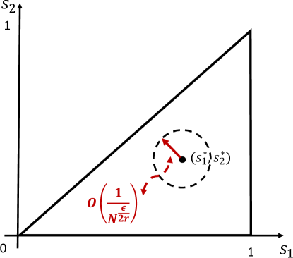
Figure 2: $b=2$ Illustration of inside region and outside region

Our analysis combines Stein’s method with a linear dynamical system and SSC. We divide the state space into two regions based on the mean-field solution; specifically, one region including the states that are “close” to the equilibrium point $s^{*},$ and the other region that includes all other states. For example, consider the case of $b=2$, so the state space is two-dimensional as shown in Figure 2, where the state space is

$$\left\{\left.(s_{1},s_{2})=\left(\frac{p}{N},\frac{q}{N}\right)\right|p\geq q\in\{0,1,\cdots,N\}\right\}\subset[0,1]^{2}.$$

As in Figure 2, we divide the state space into two regions separated by the dashed circle. The size of the circle is small and depends on $N,$ in particular, the radius is $O\left(\frac{1}{N^{\frac{\epsilon}{2r}}}\right),$ where both $\epsilon$ and $r$ are positive values (the choices of these two values become clear in the analysis).

For the two different regions, we apply different techniques:

1. We first establish higher moment bounds that upper bound the probability that the steady state is outside the dashed circle. The proof is based on the geometric tail bound in Hajek (1982), Bertsimas et al. (2001) and by showing that there is a “significant” negative drift that moves the system closer to the equilibrium point when the system is outside of the dashed circle.

2. For the states close to the equilibrium point, i.e, inside the dashed circle, from the control theory, we know that the mean-field nonlinear system behavior can be well approximated by the linearized dynamical system. By carefully choosing the parameters, we can look into the generator difference and calculate the dominant term of the approximation error by using the linearized mean-field model. The linearity enables us to solve Stein’s equation, which is a key obstacle in applying Stein’s method.

5 Simulations

Given $\alpha=0.05$, we performed simulations for two different choices of $\gamma$ and different system sizes. The purpose of these simulations is to compare the approximation errors calculated from the simulations with the asymptotically tight bound and the general upper bound. The results are based on the average of 10 runs, where each run simulates $10^{9}$ time steps. We averaged over the last $9\times 10^{8}$ time slots of each run to compute the steady state values.

For each run, we calculated the empirical mean square error multiplied by the system size $N.$ Recall that the asymptotically tight bound and upper bound are

$$-\sum_{i=1}^{b}[J^{T}(s^{*})]^{-1}_{ii}\tilde{f}_{i}(s^{*})$$

and

$$-4\sum_{i=1}^{b}[J^{T}(s^{*})]^{-1}_{ii}\tilde{f}_{i}(s^{*}),$$

respectively. Note that the two bounds only differ by a factor of four.

Table 1: $\gamma=0.1,\alpha=0.05$

$N$	10	100	1,000	10,000
$\lambda$	0.9109	0.9206	0.9292	0.9369
Simulation	4.2975	3.6884	3.9553	4.4068
Asymptotic Bound	3.2773	3.6411	4.0455	4.4955
Upper Bound	13.1092	14.5644	16.1820	17.9820

Table 2: $\gamma=0.01,\alpha=0.05$

$N$	10	100	1,000	10,000
$\lambda$	0.9911	0.9921	0.9929	0.9937
Simulation	77.9532	46.4641	38.7702	40.2093
Asymptotic Bound	28.2972	31.6293	35.3629	39.5457
Upper Bound	113.1888	126.5172	141.4516	158.1828

Tables 1 and 2 summarize the results with $\gamma=0.1,\alpha=0.05$ and $\gamma=0.01,\alpha=0.05$. We varied the size of the system in both cases. Note that the arrival rate is a function of the system size and approaches one as $N$ increases. As $N$ increases, the simulation results are in the same order with the dominant terms and are bounded by the upper bounds.

Our numerical results show that the asymptotic bound matches the empirical error very well, and approaches the empirical error as $N$ increases. In particular, for $\gamma=0.1$ and $\alpha=0.05,$ the results are close even when $N=100;$ and for $\gamma=0.01$ and $\alpha=0.05,$ the results are close when $N=1,000.$

As we can see, the upper bound is valid even for small size systems, e.g. $N=10$, which shows the effectiveness of our results. From a practical point of view, both bounds are calculable, so together, they provide good estimates of the mean-square error.

6 Proofs

As we mentioned earlier, the results are established by looking at the system in two different regions, near the equilibrium point and outside. The flow chart of the proofs is given in Figure 3.

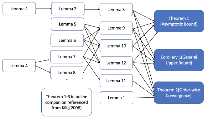
Figure 3: flowchart of proofs

6.1 State Space Concentration

First, we present some preliminary heavy-traffic convergence results for finite buffer size $b=O(\log N)$.

Lemma 6.1

For any $0<\alpha<0.25$ and a sufficiently large $N,$ we have

$$\mathbb{E}[||S-s^{*}||^{2}]\leq\frac{1}{N^{1-4\alpha-7\xi}}$$

where $\xi>0$ is an arbitrarily small number. ∎

Lemma 6.2 (Higher Moment Bounds)

For $r\in\mathbb{N}$, any $0<\alpha<0.25$ and a sufficiently large $N$, we have

$$\mathbb{E}\left[||S-s^{*}||^{2r}\right]\leq\frac{1}{N^{r(1-4\alpha-7\xi)}}$$

∎

The proofs for both lemmas are in the appendix.

Lemma 6.3 (State Space Concentration)

Letting $\epsilon>0$ and $r\in\mathbb{N}$, for a sufficiently large $N$, we have

$$\mathbb{P}\left(||S-s^{*}||^{2r}\geq\frac{1}{N^{\epsilon}}\right)\leq\frac{1}{N^{r(1-4\alpha-7\xi)-\epsilon}}$$

∎

Proof 6.4

Proof. Simply applying Markov inequality to the result of Lemma 6.2, we have

$$\mathbb{P}(||S-s^{*}||^{2r}\geq\frac{1}{N^{\epsilon}}) \leq\frac{\mathbb{E}[||S-s^{*}||^{2r}]}{\frac{1}{N^{\epsilon}}}$$

$$\leq\frac{N^{\epsilon}}{N^{r(1-4\alpha-7\xi)-\epsilon}}$$

$$=\frac{1}{N^{r(1-4\alpha-7\xi)-\epsilon}}.$$

6.2 Linear Mean-field Model

Define a set of states to be $\mathcal{B}=\{s~{}|~{}||s-s^{*}||^{2r}\leq\frac{1}{N^{\epsilon}}\},$ which are the states close to the equilibrium point. Let $d(s,s^{*})=||s-s^{*}||^{2}$ be the distance function. We consider a simple linear system

$$\dot{s}=l(s)=J(s^{*})(s-s^{*}),$$ (8)

where $J(s^{*})$ is the Jacobian matrix of $f(s)$ at the equilibrium point $s^{*}.$ In heavy-traffic, the entries of $J(s^{*})$ is generally also a function of $N$ as is $s^{*}$ itself.

The Jacobian matrix at $s$ is

$$J(s)=\left[\begin{matrix}-2\lambda s_{1}-1&1&&0\\ 2\lambda s_{1}&\ddots&\ddots&\\ &\ddots&\ddots&1\\ 0&&2\lambda s_{b-1}&-2\lambda s_{b}-1\end{matrix}\right]$$

We first introduce a lemma stating that matrix $J(s^{*})$ is invertible, i.e. $J(s^{*})^{-1}$ exists.

Lemma 6.5 (Invertibility)

For any $s\in\mathcal{S}$, the Jacobian matrix $J(s)$ is invertible.

Proof 6.6

Proof. Since it is a tridiagonal matrix, we can write down the determinant in a recursive form for $i=1,\cdots,b$,

$$P_{i}=-(2\lambda s_{i}+1)P_{i-1}-2\lambda s_{i-1}P_{i-2}$$

with initial values $P_{0}=1$ and $P_{-1}=0$, where

$$P_{i}=\left|\begin{matrix}-2\lambda s_{1}-1&1&&0\\ 2\lambda s_{1}&\ddots&\ddots&\\ &\ddots&\ddots&1\\ 0&&2\lambda s_{i-1}&-2\lambda s_{i}-1\end{matrix}\right|.$$

Furthermore, we can verify that in fact, $P_{i}$ can be written in the following form

$$P_{i}=(-1)^{i}-2\lambda s_{i}P_{i-1}$$ (9)

with $P_{1}=-(2\lambda s_{1}+1)$. We can draw two conclusions from Equation (9), for any $s\in\mathcal{S}$:

• The sign of $P_{i}$ alternates, i.e. when $i$ is odd, $P_{i}<0$; and when $i$ is even, $P_{i}>0$.

• The absolute value of $P_{i}$ is no less than 1, i.e. $|P_{i}|\geq 1.$

Because the determinant is nonzero, $J(s)$ is invertible.

Then we introduce another lemma to solve Stein’s equation (the Poisson equation) for the linear mean-field system. Consider a function $g:\mathcal{S}\to\mathcal{S}$ such that it satisfies the following equation

$$Lg(s)\dot{=}\frac{dg(s)}{dt}=\nabla g(s)\cdot l(s)=||s-s^{*}||^{2}.$$ (10)

According to the definition of the linear mean-field model in (8), we have

$$\nabla g(s)\cdot J(s^{*})(s-s^{*})=||s-s^{*}||^{2}.$$ (11)

Lemma 6.7 (Solution of Stein’s Equation)

The solution of the Poisson equation (11) satisfies

$$\nabla g(s)=[J^{T}(s^{*})]^{-1}(s-s^{*}),$$ (12)

and furthermore

$$\nabla^{2}g(s) =[J^{T}(s^{*})]^{-1}$$

$$\nabla^{3}g(s) =0.$$

Proof 6.8

Proof. According to Stein’s equation (11), we have

$$\nabla g(s)^{T}J(s^{*})(s-s^{*}) =(s-s^{*})^{T}(s-s^{*}),$$

which implies

$$\left[\nabla g(s)^{T}J(s^{*})-(s-s^{*})^{T}\right](s-s^{*}) =0.$$

Since the equation has to hold for any $s$, we have

$$\nabla g(s)^{T}J(s^{*})-(s-s^{*})^{T}=0,$$

which implies

$$\nabla g(s)=[J^{T}(s^{*})]^{-1}(s-s^{*}).$$

The higher-order derivatives follow.

6.3 Proof of the theorem

We start from the mean square error by studying the generator difference when state $S$ is close to $s^{*}.$ In particular, we focus on

$$\mathbb{E}\left[Lg(S)-Gg(S)\left|S\in\mathcal{B}\right.\right].$$ (13)

Lemma 6.9

The generator applying to function $g(s)$ satisfies

$$Gg(s)=\nabla g(s)\cdot f(s)+\frac{1}{N}\sum_{i=1}^{b}\nabla^{2}g(s)_{ii}\tilde{f}_{i}(s)$$ (14)

where $\nabla^{2}g(s)_{ii}$ is the $i$-th diagonal element of the Hessian matrix $\nabla^{2}g(s)$ and

$$\tilde{f}_{i}(s)=\frac{1}{2}[\lambda(s^{2}_{i-1}-s^{2}_{i})+(s_{i}-s_{i+1})].$$

Proof 6.10

Proof. According to the definition of generator $G,$ we have

$$Gg(s)= \sum_{i=1}^{b}\lambda N(s^{2}_{i-1}-s^{2}_{i})[g(s+e_{i})-g(s)]+N(s_{i}-s_{i+1})[g(s-e_{i})-g(s)].$$

By the Taylor expansion at the state $s,$ we have

$$Gg(s)= \sum_{i=1}^{b}\lambda N(s^{2}_{i-1}-s^{2}_{i})[\nabla g(s)\cdot e_{i}+\frac{1}{2}e_{i}^{T}\nabla^{2}g(s)e_{i}]+N(s_{i}-s_{i+1})[\nabla g(s)\cdot(-e_{i})+\frac{1}{2}e_{i}^{T}\nabla^{2}g(s)e_{i}]$$

$$= \sum_{i=1}^{b}\nabla g(s)\cdot[\lambda(s^{2}_{i-1}-s^{2}_{i})-(s_{i}-s_{i+1})]Ne_{i}+\frac{1}{2}Ne_{i}^{T}\nabla^{2}g(s)e_{i}[\lambda(s^{2}_{i-1}-s^{2}_{i})+(s_{i}-s_{i+1})]$$

$$= \nabla g(s)\cdot f(s)+\frac{1}{N}\sum_{i=1}^{b}\nabla^{2}g(s)_{ii}\tilde{f}_{i}(s).$$

The first equality holds because $\nabla^{3}g(s)=0$ according to Lemma 6.7.

When the state $s$ is close to the equilibrium point $s^{*}$ in particular assuming $||s-s^{*}||^{2r}\leq\frac{1}{N^{\epsilon}}$, we define

$$x_{i}=s_{i}-s^{*}_{i}$$

and have the Taylor expansion of $\tilde{f}_{i}(s)$ at the equilibrium point $s^{*}$

$$\tilde{f}_{i}(s)= \frac{1}{2}[\lambda(s^{2}_{i-1}-s^{2}_{i})+(s_{i}-s_{i+1})]$$

$$= \frac{\lambda}{2}[(s^{*}_{i-1}+x_{i-1})^{2}-(s^{*}_{i}+x_{i})^{2}]+\frac{1}{2}(s^{*}_{i}+x_{i}-s^{*}_{i+1}-x_{i+1})$$

$$= \frac{\lambda}{2}[(s^{*}_{i-1})^{2}+2x_{i-1}s^{*}_{i-1}+x_{i-1}^{2}-(s^{*}_{i})^{2}-2x_{i}s^{*}_{i}-x_{i}^{2}]+\frac{1}{2}(s^{*}_{i}+x_{i}-s^{*}_{i+1}-x_{i+1})$$

$$= \frac{\lambda}{2}[(s^{*}_{i-1})^{2}-(s^{*}_{i})^{2}]+\frac{1}{2}(s^{*}_{i}-s^{*}_{i+1})+O(\frac{1}{N^{\frac{\epsilon}{2r}}})$$

$$= \tilde{f}_{i}(s^{*})+O(\frac{1}{N^{\frac{\epsilon}{2r}}}),$$ (15)

where the last equality holds because $||s-s^{*}||^{2r}\leq\frac{1}{N^{\epsilon}}$ implies $|x_{i}|\leq\frac{1}{N^{\frac{\epsilon}{2r}}}.$

Consider a state $s,$ which is close to the equilibrium point, i.e. $\|s-s^{*}\|^{2r}\leq\frac{1}{N^{\epsilon}}.$ According to Stein’s equation (11) and the previous lemma, we have

$$Lg(s)-Gg(s)$$

$$= \nabla g(s)\cdot J(s^{*})(s-s^{*})-\nabla g(s)\cdot f(s)-\frac{1}{N}\sum_{i=1}^{b}\nabla^{2}g(s)_{ii}\tilde{f}_{i}(s)$$

$$= \nabla g(s)\cdot\left(J(s^{*})(s-s^{*})-f(s)\right)-\frac{1}{N}\sum_{i=1}^{b}\nabla^{2}g(s)_{ii}\left(\tilde{f}_{i}(s^{*})+O\left(\frac{1}{N^{\frac{\epsilon}{2r}}}\right)\right)$$

$$= \nabla g(s)\cdot\left(J(s^{*})(s-s^{*})-f(s)\right)-\frac{1}{N}\sum_{i=1}^{b}\nabla^{2}g(s)_{ii}\tilde{f}_{i}(s^{*})-\frac{1}{N}\sum_{i=1}^{b}\nabla^{2}g(s)_{ii}O\left(\frac{1}{N^{\frac{\epsilon}{2r}}}\right).$$

According to Lemma 6.7, we have

$$\nabla g(s) =[J^{T}(s^{*})]^{-1}(s-s^{*}),$$

$$\nabla^{2}g(s) =[J^{T}(s^{*})]^{-1},$$

which are the functions of $J(s^{*}).$

Since the original mean-field is a second-order system, we have

$$f(s)= f(s^{*})+J(s^{*})(s-s^{*})+\frac{1}{2}<s-s^{*},\nabla^{2}f(s^{*})(s-s^{*})>,$$

where $\nabla^{2}f(s^{*})$ is the Hessian of $f(s)$ at equilibrium point. For any $s\in\mathcal{S}$ and $i=1,\cdots,b$, the Hessian has the following form for $f_{i}(s)$

$$\nabla^{2}f_{i}(s)_{kj}=\frac{\partial^{2}f_{i}(s)}{\partial s_{j}\partial s_{k}}=\begin{cases}-2\lambda,&\text{if }j=k=i,\\ 2\lambda,&\text{if }j=k=i-1,\\ 0,&\text{otherwise}.\end{cases}$$

Substituting it into the generator difference, we obtain

$$\mathbb{E}\left[Lg(S)-Gg(S)~{}\big{\rvert}~{}S\in\mathcal{B}\right]$$

$$= \mathbb{E}\big{[}[J^{T}(s^{*})]^{-1}(S-s^{*})\cdot(\frac{1}{2}<S-s^{*},\nabla^{2}f(s^{*})(S-s^{*})>)$$

$$\quad-\frac{1}{N}\sum_{i=1}^{b}\nabla^{2}g(S)_{ii}\tilde{f}_{i}(s^{*})-\frac{1}{N}\sum_{i=1}^{b}\nabla^{2}g(S)_{ii}O(\frac{1}{N^{\frac{\epsilon}{2r}}})~{}\big{\rvert}~{}S\in\mathcal{B}\big{]}.$$ (16)

This generator difference includes three terms. Note that $\nabla^{2}g(s)=[J^{T}(s^{*})]^{-1}=[J^{-1}(s^{*})]^{T}$, according to Lemma 6.7.

We next introduce two lemmas with regard to matrix $J^{-1}(s^{*})$, which is involved in all three terms in Equation (16).

Lemma 6.11 (Upper Bound on the Elements of Matrix $J^{-1}(s^{*})$)

For all $i,j=1,\cdots,b$ and a sufficiently large $N$, we have

$$|[J(s^{*})]^{-1}_{ij}|\leq\frac{12}{\gamma}N^{2\alpha+2\xi}.$$

∎

Lemma 6.12 (Lower Bound on a Diagonal Element of Matrix $J^{-1}(s^{*})$)

For tridiagonal matrix $J^{-1}(s^{*})$, we have that

$$|J^{-1}_{11}(s^{*})|\geq\frac{1}{3}$$ (17)

and for all $i=1,\cdots,b$, we have $J^{-1}_{ii}(s^{*})<0$.∎

The proofs of these lemmas can be found in appendix. Based on lemmas 6.11 and 6.12, we have the following lemmas to bound the terms in (16).

Lemma 6.13

Given $||s-s^{*}||^{2r}\leq\frac{1}{N^{\epsilon}}$, we have

$$||[J^{T}(s^{*})]^{-1}(s-s^{*})\cdot<s-s^{*},\nabla^{2}f(s^{*})(s-s^{*})>||$$

$$\quad=O\left(\frac{1}{N^{\frac{3\epsilon}{2r}-2\alpha-3\xi}}\right).$$ (18)

Proof 6.14

Proof. Consider the 2-norm of the first term in (16). We have

$$||[J^{T}(s^{*})]^{-1}(s-s^{*})\cdot<s-s^{*},\nabla^{2}f(s^{*})(s-s^{*})>||$$

$$\leq ||[J^{T}(s^{*})]^{-1}(s-s^{*})||||<s-s^{*},\nabla^{2}f(s^{*})(s-s^{*})>||$$

$$\leq ||[J^{T}(s^{*})]^{-1}||||s-s^{*}||||<s-s^{*},\nabla^{2}f(s^{*})(s-s^{*})>||$$

$$\leq 2\sqrt{2}\lambda||[J^{T}(s^{*})]^{-1}||||s-s^{*}||^{3},$$ (19)

where the third inequality holds because

$$\begin{split}&||<s-s^{*},\nabla^{2}f(s^{*})(s-s^{*})>||\\ =&\sqrt{\sum_{i=1}^{b}[(s-s^{*})\nabla^{2}f_{i}(s^{*})(s-s^{*})]^{2}}\\ =&\sqrt{\sum_{i=1}^{b}\left(2\lambda[(s_{i-1}-s^{*}_{i-1})^{2}-(s_{i}-s^{*}_{i})^{2}]\right)^{2}}\\ =&2\lambda\sqrt{\sum_{i=1}^{b}[(s_{i-1}-s^{*}_{i-1})^{2}-(s_{i}-s^{*}_{i})^{2}]^{2}}\\ \leq&2\lambda\sqrt{\sum_{i=1}^{b}(s_{i-1}-s^{*}_{i-1})^{4}+(s_{i}-s^{*}_{i})^{4}}\\ \leq&2\sqrt{2}\lambda\sqrt{\sum_{i=1}^{b}(s_{i}-s^{*}_{i})^{4}}\\ \leq&2\sqrt{2}\lambda\sqrt{[\sum_{i=1}^{b}(s_{i}-s^{*}_{i})^{2}]^{2}}\\ =&2\sqrt{2}\lambda||s-s^{*}||^{2}.\end{split}$$

Furthermore, from Lemma 6.11, for a sufficiently large $N$, we have

$$||[J^{T}(s^{*})]^{-1}||=||[J(s^{*})]^{-1}||\leq \max_{ij}|[J(s^{*})]^{-1}_{ij}|\times b$$

$$= O(N^{2\alpha+2\xi})\times O(\log N)$$

$$= O(N^{2\alpha+3\xi}).$$ (20)

Since $||s-s^{*}||^{2r}\leq\frac{1}{N^{\epsilon}}$, combining inequalities (19) and (20), we have

$$||[J^{T}(s^{*})]^{-1}(s-s^{*})\cdot<s-s^{*},\nabla^{2}f(s^{*})(s-s^{*})>||$$

$$\leq 2\sqrt{2}\lambda\times O\left(N^{2\alpha+3\xi}\right)\times\frac{1}{N^{\frac{3\epsilon}{2r}}}=O\left(\frac{1}{N^{\frac{3\epsilon}{2r}-2\alpha-3\xi}}\right).$$

Lemma 6.15

Given $||s-s^{*}||^{2r}\leq\frac{1}{N^{\epsilon}}$, we have

$$-\frac{1}{N}\sum_{i=1}^{b}\nabla^{2}g_{ii}(s)\tilde{f}_{i}(s^{*}) \geq\frac{\lambda\gamma}{3N^{1+\alpha}}.$$ (21)

Proof 6.16

Proof. Recall that $\nabla^{2}g(s)=[J^{T}(s^{*})]^{-1}$ and for $i=1,\cdots,b$, $J^{-1}(s^{*})_{ii}<0$ according to Lemma 6.12. It is easy to check that for $i=1,\cdots,b$, $\tilde{f}_{i}(s^{*})\geq 0$.Therefore, for $i=1,\cdots,b$, we have

$$-\nabla^{2}g(s)_{ii}\tilde{f}_{i}(s^{*})\geq 0.$$

Furthermore, we also have

$$\tilde{f}_{i}(s^{*}) =\frac{1}{2}[\lambda((s^{*}_{i-1})^{2}-(s^{*}_{i})^{2})+(s^{*}_{i}-s^{*}_{i+1})]$$

$$=\lambda[(s^{*}_{i-1})^{2}-(s^{*}_{i})^{2}],$$

where the second equality holds because $s^{*}$ is the equilibrium point. Thus, for $i=1$ by equation (1b), we have

$$\tilde{f}_{1}(s^{*})=\lambda[1-(s^{*}_{1})^{2}] \geq\lambda(1-\lambda^{2})\geq\lambda(1-\lambda)=\frac{\lambda\gamma}{N^{\alpha}}$$

which implies

$$\frac{1}{N}\sum_{i=1}^{b}\nabla^{2}g_{ii}(s)\tilde{f}_{i}(s^{*}) \geq-\frac{1}{N}J^{-1}_{11}(s^{*})\tilde{f}_{1}(s^{*})\geq\frac{\lambda\gamma}{3N^{1+\alpha}}.$$

Lemma 6.17

Given $||s-s^{*}||^{2r}\leq\frac{1}{N^{\epsilon}}$, we have

$$-\frac{1}{N}\sum_{i=1}^{b}\nabla^{2}g_{ii}(s)\tilde{f}_{i}(s^{*})=O(\frac{1}{N^{1-2\alpha-3\xi}}).$$ (22)

Proof 6.18

Proof. It is easy to check that $\tilde{f}_{i}(s^{*})\leq 1$ for $i=1,\cdots,b$. Recall that $|\nabla^{2}g(s)_{ii}|\leq O(N^{2\alpha+2\xi})$. Therefore, we have

$$-\frac{1}{N}\sum_{i=1}^{b}\nabla^{2}g_{ii}(s)\tilde{f}_{i}(s^{*})$$

$$= \frac{b}{N}O(N^{2\alpha+2\xi})=O(\frac{1}{N^{1-2\alpha-3\xi}}).$$

Lemma 6.19

Given $||s-s^{*}||^{2r}\leq\frac{1}{N^{\epsilon}}$, we have that for a sufficiently large $N$,

$$\left\|-\frac{1}{N}\sum_{i=1}^{b}\nabla^{2}g(s)_{ii}O(\frac{1}{N^{\frac{\epsilon}{2r}}})\right\|=O\left(\frac{1}{N^{1+\frac{\epsilon}{2r}-2\alpha-3\xi}}\right).$$ (23)

Proof 6.20

Proof. Recall that $|\nabla^{2}g(s)_{ii}|=O(N^{2\alpha+2\xi})$ for $i=1,\cdots,b$. Thus, we have

$$||-\frac{1}{N}\sum_{i=1}^{b}\nabla^{2}g(s)_{ii}O(\frac{1}{N^{\frac{\epsilon}{2r}}})||$$

$$\leq \frac{b}{N}O(N^{2\alpha+2\xi})\cdot O(\frac{1}{N^{\frac{\epsilon}{2r}}})$$

$$= O(\frac{1}{N^{1+\frac{\epsilon}{2r}-2\alpha-3\xi}}).$$

Based on these lemmas, we are now able to characterize the generator difference when state $S$ is close to $s^{*}.$

Lemma 6.21

For $0<\alpha<\frac{1}{18}$ and a sufficiently large $N$, we have

$$\mathbb{E}\left[Lg(S)-Gg(S)\left|S\in\mathcal{B}\right.\right]=-\frac{1}{N}\sum_{i=1}^{b}[J^{T}(s^{*})]^{-1}_{ii}\tilde{f}_{i}(s^{*})+o\left(\frac{1}{N^{1+\alpha}}\right),$$ (24)

with the following choice of parameters

$$\frac{3(1+\alpha+\xi)}{1-18\alpha-27\xi} <r,$$ (25)

$$\frac{2r(1+3\alpha+3\xi)}{3} <\epsilon<r(1-4\alpha-7\xi)-1-\alpha-\xi.$$ (26)

Proof 6.22

Proof. Under the conditions of the lemma, it is easy to check that the upper bound of the first and third terms in equation (16) are order-wise smaller than the lower bounds of the second term, i.e.

$$\frac{3\epsilon}{2r}-2\alpha-3\xi>1+3\alpha+3\xi-2\alpha-3\xi=1+\alpha$$

and

$$1+\frac{\epsilon}{2r}-2\alpha-3\xi >1+\frac{1}{3}+\alpha+\xi-2\alpha-3\xi$$

$$>(1+\alpha)+(\frac{2}{9}-2\xi),$$

where the last inequality is by the fact $0<\alpha<\frac{1}{18}$. Therefore, the lemma holds.

We also remark that there exist parameters that satisfy the conditions in the lemma because the right-hand side of $\epsilon$ in (26) is larger than the left-hand side given that the $r$ satisfies (25), where $r$ has to be large enough. For example, when $\alpha=0.05$, $r$ needs to at least 32 and $\epsilon$ can be $24.54$, and it’s easy to check that we can find a small enough $\xi$.

6.4 Proof of Theorem 4.1

We again choose parameters that satisfy the following conditions:

$$\frac{3(1+\alpha)}{1-18\alpha-27\xi} <r$$

$$\frac{2r(1+3\alpha+3\xi)}{3} <\epsilon<r(1-4\alpha-7\xi)-1-\alpha-\xi$$

and $\xi>0$ is arbitrarily small. Then, for a sufficiently large $N$, the mean square distance is

$$\mathbb{E}[||S-s^{*}||^{2}]$$

$$= \mathbb{E}\left[||S-s^{*}||^{2}\big{\rvert}S\notin\mathcal{B}\right]\mathbb{P}\left(S\notin\mathcal{B}\right)+\mathbb{E}\left[||S-s^{*}||^{2}\big{\rvert}S\in\mathcal{B}\right]\mathbb{P}\left(S\in\mathcal{B}\right)$$

$$= O(\log N)\times O(\frac{1}{N^{r(1-4\alpha-7\xi)-\epsilon}})+\left(-\frac{1}{N}\sum_{i=1}^{b}\nabla^{2}g(s)_{ii}\tilde{f}_{i}(s^{*})+o(\frac{1}{N^{1+\alpha}})\right)\times\left(1-O(\frac{1}{N^{r(1-4\alpha-7\xi)-\epsilon}})\right)$$

$$= O\left(\frac{1}{N^{r(1-4\alpha-7\xi)-\epsilon-\xi}}\right)-\frac{1}{N}\sum_{i=1}^{b}\nabla^{2}g(s)_{ii}\tilde{f}_{i}(s^{*})+O\left(\frac{1}{N^{1-2\alpha-3\xi}}\right)\times O\left(\frac{1}{N^{r(1-4\alpha-7\xi)-\epsilon}}\right)+o\left(\frac{1}{N^{1+\alpha}}\right)$$

$$= -\frac{1}{N}\sum_{i=1}^{b}[J^{T}(s^{*})]^{-1}_{ii}\tilde{f}_{i}(s^{*})+o\left(\frac{1}{N^{1+\alpha}}\right),$$

where the second equality holds because $||s-s^{*}||^{2}\leq b=O(\log N).$ Note that with the choice of parameters $r,\epsilon$ and $0<\alpha<\frac{1}{18},$ the lower bound of the term $-\frac{1}{N}\sum_{i=1}^{b}[J^{T}(s^{*})]^{-1}_{ii}\tilde{f}_{i}(s^{*})+o(\frac{1}{N^{1+\alpha}})$ is $O(\frac{1}{N^{1+\alpha}})$, while the other terms are strictly upper bounded by this order for sufficiently large $N$.

6.5 Proof of the Corollary 4.2

From Lemma 6.21 with the same parameter choices, it is easy to check that for sufficiently large $N$, we have

$$\mathbb{E}\left[Lg(S)-Gg(S)\left|S\in\mathcal{B}\right.\right]$$ (27)

$$\leq -\frac{3}{N}\sum_{i=1}^{b}[J^{T}(s^{*})]^{-1}_{ii}\tilde{f}_{i}(s^{*}).$$

Also, the following holds for a sufficiently large $N$,

$$\mathbb{P}\left(||S-s^{*}||^{2r}\geq\frac{1}{N^{\epsilon}}\right)\leq\frac{1}{N^{r(1-4\alpha-\xi^{{}^{\prime}})-\epsilon}}\leq\frac{1}{N^{1+\alpha+\xi}}.$$

Then from the above two inequalities, for a sufficiently large $N$, the mean square distance is

$$\mathbb{E}[||S-s^{*}||^{2}]$$

$$= \mathbb{E}\left[Lg(S)-Gg(S)\big{\rvert}S\notin\mathcal{B}\right]\mathbb{P}\left(S\notin\mathcal{B}\right)+\mathbb{E}\left[Lg(S)-Gg(S)\big{\rvert}S\in\mathcal{B}\right]\mathbb{P}\left(S\in\mathcal{B}\right)$$

$$\leq \frac{b}{N^{1+\alpha+\xi}}-\frac{3}{N}\sum_{i=1}^{b}[J^{T}(s^{*})]^{-1}_{ii}\tilde{f}_{i}(s^{*})$$

$$\leq \frac{1}{N^{1+\alpha}}-\frac{3}{N}\sum_{i=1}^{b}[J^{T}(s^{*})]^{-1}_{ii}\tilde{f}_{i}(s^{*})$$

$$\leq -\frac{4}{N}\sum_{i=1}^{b}[J^{T}(s^{*})]^{-1}_{ii}\tilde{f}_{i}(s^{*}),$$

where the second from the last inequality holds because the first term is larger than the right-hand side of inequality (21).

6.6 Proof of the Theorem 4.3

We choose following parameter choices

$$\frac{3(1-2\alpha-2\xi)}{1-12\alpha-21\xi}\leq r$$ (28)

$$\frac{2r}{3}\leq\epsilon\leq r(1-4\alpha-7\xi)-1-\alpha-\xi$$

and $\xi>0$ is arbitrarily small. For $\alpha\in(0,1/12)$, similar to the proof of Theorem 4.1, we show that the term in equation (22) in Lemma 6.17 is the dominant term. It is easy to check for $s\in\mathcal{B}$ that

$$\mathbb{E}\left[Lg(S)-Gg(S)\left|S\in\mathcal{B}\right.\right]=O(\frac{1}{N^{1-2\alpha-3\xi}}).$$ (29)

Combined with the probability of $s\notin\mathcal{B}$ and equation (29), for sufficiently large $N$, we have the mean square error as

$$\mathbb{E}[||S-s^{*}||^{2}]$$

$$= \mathbb{E}\left[||S-s^{*}||^{2}\big{\rvert}S\notin\mathcal{B}\right]\mathbb{P}\left(S\notin\mathcal{B}\right)+\mathbb{E}\left[||S-s^{*}||^{2}\big{\rvert}S\in\mathcal{B}\right]\mathbb{P}\left(S\in\mathcal{B}\right)$$

$$= O(\log N)\times O(\frac{1}{N^{r(1-4\alpha-7\xi)-\epsilon}})+O(\frac{1}{N^{1-2\alpha-3\xi}})\times\left(1-O(\frac{1}{N^{r(1-4\alpha-7\xi)-\epsilon}})\right)$$

$$= O\left(\frac{1}{N^{r(1-4\alpha-7\xi)-\epsilon-\xi}}\right)+O(\frac{1}{N^{1-2\alpha-3\xi}})$$

$$= O(\frac{1}{N^{1-2\alpha-3\xi}})$$

where the last equality is the result of the parameter choices. We note that the requirement for $\alpha<\frac{1}{12}$ results from the fact that the denominator of LHS of inequality (28) needs to be positive.

Together with Lemma 6.1, we conclude the proof for all $\alpha\in(0,0.25)$, hence the Theorem 4.3 holds.

7 Conclusion

In this paper, we established calculable bounds on the mean-square errors of the power-of-two-choices mean-field model in heavy-traffic. Our approach combined SSC and Stein’s method with a linearized mean-field models, and characterized the dominant term of the mean square error. Our simulation results confirmed the theoretical bounds and showed that the bounds are valid even for small size systems such as when $N=10.$ This recipe of combining SSC and Stein’s method for linearized mean-field model can be applied to other mean-field models beyond the power-of-two-choices load balancing algorithm.

8 Proof of Lemma 6.1

Lemma 8.1

For $\lambda=1-\frac{\gamma}{N^{\alpha}}$ and $\lambda>0.75$, given $0<\alpha<0.25,0<\gamma\leq 1$, when $N$ is sufficiently large, we have

$$\mathbb{E}[||S-s^{*}||^{2}]\leq\frac{1}{N^{1-4\alpha-7\xi}}$$

where $\xi>0$ can be chosen arbitrarily small.

The proof and analysis follow from the heavy-traffic infinite buffer size case in Ying (2017). We remark that the differences between the mean-field model here and the truncated mean-field model in Ying (2017) are the dimension and the last equation. Specifically, we used dimension $b=O(\log N)$ and the truncated system considers $N^{\alpha+\xi}$ dimensional system, where $\xi>0$ is arbitrarily small; for the dynamical equation in the last dimension, we don’t have an added term and, in Ying (2017), a term is added so that the solution of the mean-field model can be written in a closed form. For finite buffer size with $b=O(\log N)$, the mean-field model is the following

$$\dot{s}_{k}=\begin{cases}\lambda(s^{2}_{k-1}-s^{2}_{k})-(s_{k}-s_{k+1}),&b-1\leq k\leq 1\\ \lambda(s^{2}_{b-1}-s^{2}_{b})-s_{b},&k=b\end{cases}$$

where $s_{0}(t)=1$ and $s_{b+1}(t)=0$ for $t\geq 0$. There exists a unique equilibrium points $\{s^{*}_{k}\}_{k=1,\cdots,b}$. We next establish the upper bound on

$$\mathbb{E}[||X||^{2}]$$

where $X=S-s^{*}$ and the expectation is taken over the stationary distribution. Let $\mathcal{X}$ be the state space of $X$.

Define $x=s-s^{*}$, so

$$\dot{x}_{k}=f_{k}(x) :=\begin{cases}\lambda[(x_{k-1}+s^{*}_{k-1})^{2}-(x_{k}+s^{*}_{k})^{2})]-[(x_{k}+s^{*}_{k})-(x_{k+1}+s^{*}_{k+1})],&1\leq k\leq b-1\\ \lambda[(x_{b-1}+s^{*}_{b-1})^{2}-(x_{b}+s^{*}_{b})^{2}]-(x_{b}+s^{*}_{b}),&k=b\end{cases}$$

$$=\begin{cases}-\lambda(x^{2}_{1}+2s^{*}_{1}x_{1})-(x_{1}-x_{2}),&k=1\\ \lambda[(x^{2}_{k-1}+2s^{*}_{k-1}x_{k-1})-(x^{2}_{k}+2s^{*}_{k}x_{k})]-(x_{k}-x_{k+1}),&2\leq k\leq b-1\\ \lambda[(x^{2}_{b-1}+2s^{*}_{b-1}x_{b-1})-(x^{2}_{b}+2s^{*}_{b}x_{b})]-x_{b},&k=b.\end{cases}$$ (30)

The unique equilibrium point for the system is $x^{*}=0$. Consider $d(x,x^{*})=\sum_{i=1}^{b}x^{2}_{k}$. In this case, define

$$g_{h}(x)=-\int_{0}^{\infty}\sum_{k=1}^{b}x^{2}_{k}(t,x)dt$$

where $x(t,x)$ denotes the trajectory of the mean-field dynamical system with $x$ as the initial condition and is the solution for the dynamical system defined in (30). By combining the Poisson equation and the steady-state equation, we have

$$\mathbb{E}[\sum_{k=1}^{b}X^{2}_{k}]=\mathbb{E}[\nabla g_{h}(X)\cdot f(X)-Gg_{h}(X)].$$

From the definitions of $f_{k}$ and $R_{x,y}$, we have

$$f_{k}(x)=\sum_{y\neq x}R_{x,y}(y_{k}-x_{k})$$

for $k=1,\cdots,b$. So

$$\nabla g_{h}(x)\cdot f(x) =\sum_{k=1}^{b}\frac{\partial g_{h}}{\partial x_{k}}[\sum_{y\neq x}R_{x,y}(y_{k}-x_{k})]$$

$$=\sum_{y\neq x}R_{x,y}\sum_{k=1}^{b}\frac{\partial g_{h}}{\partial x_{k}}(y_{k}-x_{k})$$

$$=\sum_{y\neq x}R_{x,y}\nabla g_{h}(x)\cdot(y-x).$$

Therefore, we have the following equation

$$\mathbb{E}[\sum_{k=1}^{b}X^{2}_{k}]=\mathbb{E}[-\sum_{y\neq X}R_{X,y}\Gamma_{h}(X,y)]$$ (31)

where $\Gamma_{h}(X,y)=g_{h}(y)-g_{h}(X)-\nabla g_{h}(X)\cdot(y-x)$. We just need to establish a bound on $\Gamma_{h}(X,y)$. In the following section, we introduce the gradient bound for mean-field model, from which we can provide a bound on $\Gamma_{h}(X,y)$.

8.1 Gradient Bound for Mean-Field Model

In the following part, we establish a gradient bound for the-power-of-two-choices by applying Lemma 2.2 of Ying (2017) to our $b$-dimensional system. We restate the lemma here for your convenience and adapt to our notations.

Following the analysis in Ying (2016), we consider the following collection of dynamical systems:

$$\dot{e}(t) =f(x(t,z))-f(x(t,z))-\frac{1}{N}\frac{\partial f}{\partial x}(x(t,y))x^{(1)}(t)$$ (32)

$$\dot{x}^{(1)}(t) =\frac{\partial f}{\partial x}(x(t,y))x^{(1)}(t)$$ (33)

$$\dot{x}(t,y) =f(x(t,y))$$ (34)

$$\dot{x}(t,z) =f(x(t,z))$$ (35)

with initial conditions $e(0)=0,x^{(1)}(0)=N(z-y),x(0,z)=z$ and $x(0,y)=y$, where $\frac{\partial f}{\partial x}$ denotes the Jacobian matrix.

Lemma 8.2 (Gradient Bound For Mean-Field Models)

Assume the following conditions hold:

C 1

Given initial condition $z$ and any positive constant $\tilde{d}$, there exists $\tilde{t}_{\tilde{d},z}$ such that

$$|x(t,z)|\leq\tilde{d}\qquad\forall t\geq\tilde{t}_{\tilde{d},z}.$$

C 2

There exists a constant $c_{1}$ such that

$$x^{(1)}(t)\leq c_{1}|x^{(1)}(t)|\qquad\forall t.$$

C 3

There exist Lyapunov function $V_{1}(x^{(1)})$ and positive constants $c_{u1},c_{l1},d_{1}$ and $\delta_{1}$ such that

(1) $c_{l1}|x^{(1)}|\leq V_{1}(x^{(1)})\leq c_{u1}|x^{(1)}|$, and

(2) when $|x(t,z)|\leq d_{1}$,

$$\dot{V}_{1}(x^{(1)}(t))\leq-\delta_{1}V_{1}(x^{(1)}(t)).$$

C 4

There exists a positive constant $c_{e}$ such that given $|e(t)|\leq\frac{1}{N}$,

$$\frac{d|e(t)|}{dt}\leq\frac{c_{e}}{N^{2}}.$$

C 5

There exists Lyapunov function $V_{e}(e)$ and positive constants $c_{er},\delta_{e},d_{e}$ and $\alpha_{e}$ such that

(1) $c_{le}(e)|e|\leq V_{e}(e)\leq c_{ue}|e|$, and

(2) when $|x(t,z)|\leq d_{e}$,

$$\dot{V}_{e}(e(t))\leq-\delta_{e}V_{e}(e(t))+\frac{c_{er}}{N^{2}}|x^{(1)}(t)|^{\alpha_{e}}.$$

C 6

There exists constant $c_{2}$ such that $x^{(1)}(0)=N(z-y)\leq c_{2}$ for any $y,z\in\mathcal{X}$. Furthermore, $\tilde{t}_{d_{1},x}=o(N)$ and $\tilde{t}_{d_{e},x}=o(N)$ for any $x\in\mathcal{X}$, which is the state space.

C 7

The following constants are independent of $N$: $c_{1},c_{l1},c_{u1},c_{le},c_{ue},c_{e},c_{er},\alpha_{e}$ and $c_{2}$.

Then there exists a positive constant $\kappa$, independent of $N$, such that when $N$ is sufficiently large,

$$\int_{0}^{\infty}|x^{(1)}(t)|^{2}dt \leq\kappa(\tilde{t}_{d,z}+\frac{1}{\delta_{1}})$$ (36)

$$\int_{0}^{\infty}|e(t)|dt \leq\kappa(\frac{\tilde{t}_{d,z}}{\delta_{e}}+\frac{1}{\delta_{1}\delta_{e}}+\tilde{t}^{2}_{d,z})\frac{1}{N^{2}}$$ (37)

where $d=\min\{d_{1},d_{e}\}$.

This lemma above provides bounds on $\int_{0}^{\infty}|x^{(1)}(t)|dt$ and $\int_{0}^{\infty}|e(t)|dt$, which can be used to bound $\Gamma_{h}(z,y)$. Since we use 2-norm as the distance measure, we will have

$$|\Gamma_{h}(z,y)|\leq\int_{0}^{\infty}\left(3x_{\max}|e(t)|+\frac{1}{N^{2}}|x^{(1)}(t)|^{2}\right)dt$$ (38)

where $x_{\max}$ is a constant such that $x_{i}\leq x_{\max}$ for any $x\in\mathcal{X}$ and any $i$.

8.2 Verifying the Conditions for Gradient Bound

The following analysis and lemmas are to lay the groundwork for verifying the conditions to apply the gradient bound for mean-field model.

Given an arbitrarily small $\xi>0$, define

$$\tilde{k}=(\alpha+\xi)\log_{2}N.$$

Without loss of generality, we assume $b\geq\tilde{k}$.

Lemma 8.3

According to the definition of $\tilde{k}$, for sufficiently large $N$, we have for any $k\geq\tilde{k}$

$$\lambda(s^{*}_{k}+1)\leq\lambda(\lambda^{2^{k}-1}+1)\leq\sqrt{\lambda}.$$

Proof 8.4

Proof. The equilibrium point of the mean-field system satisfies the following equations

$$\lambda[(s^{*}_{k-1})^{2}-(s^{*}_{k})^{2}]-(s^{*}_{k}-s^{*}_{k+1})=0,\quad 1\leq k\leq b-1$$

$$\lambda[(s^{*}_{b-1})^{2}-(s^{*}_{b})^{2}]-s^{*}_{b}=0,\quad k=b.$$

For any $k$ that is $1\leq k\leq b-1$, by adding equation $(k)$ to $(b)$, we have

$$\lambda[(s^{*}_{k-1})^{2}-(s^{*}_{b})^{2}]-s^{*}_{k}=0.$$

Thus, we have

$$s^{*}_{k}=\lambda[(s^{*}_{k-1})^{2}-(s^{*}_{b})^{2}]\leq\lambda(s^{*}_{k-1})^{2}.$$

The equation (b) is equivalent to

$$s^{*}_{b}+\lambda(s^{*}_{b})^{2}=\lambda(s^{*}_{b-1})^{2}.$$

As a result, for $k=b$, we also have inequality

$$s^{*}_{k}\leq\lambda(s^{*}_{k-1})^{2}.$$

So iteratively, given $s^{*}_{0}=1$, for all $1\leq k\leq b$,

$$s^{*}_{k}\leq\lambda^{2^{k}-1}.$$

The first inequality follows as a result.

For the second inequality, note that

$$\lambda^{2^{k}}\leq\lambda^{2^{\tilde{k}}}=\lambda^{N^{\alpha+\xi}}=(1-\frac{\gamma}{N^{\alpha}})^{N^{\alpha+\xi}},$$

so

$$\log\lambda^{2^{k}}\leq N^{\alpha+\xi}\log(1-\frac{\gamma}{N^{\alpha}})\leq_{(a)}-\gamma N^{\xi}=-\Theta(N^{\xi}),$$

where inequality (a) is a result of the Taylor expansion. Furthermore,

$$\log(\sqrt{\lambda}-\lambda)=\log\sqrt{\lambda}+\log(1-\sqrt{\lambda})=-\Theta(\alpha\log N).$$

Therefore, for sufficiently large $N$, we have

$$\lambda^{2^{k}}\leq\sqrt{\lambda}-\lambda,$$

and the lemma holds.

Now define a sequence of $\{w_{k}\}$ such that for some $\epsilon>0$

$$w_{0} =0$$

$$w_{1} =1$$

$$w_{k} =1+\frac{1}{2}\sum_{j=1}^{k}\frac{1}{(2\lambda+\epsilon)^{j-1}},\quad 2\leq k\leq\tilde{k}$$

$$w_{k} =w_{\tilde{k}}+\frac{k-\tilde{k}}{2(2\lambda+\epsilon)^{\tilde{k}}},\quad\tilde{k}<k\leq b.$$

We choose a constant $\epsilon$ independent of $N$ such that

$$\min\{0.5,2^{\frac{\alpha+2\xi}{\alpha+\xi}}-2\lambda\}>\epsilon>2-2\lambda.$$

Such an $\epsilon$ exists when $\lambda>0.75$. Note that in heavy-traffic regime, we consider arrival rate that approaches 1, so $\lambda>0.75$ is easy to be satisfied. We further define

$$\delta_{0}=\frac{1-\sqrt{\lambda}}{6(2\lambda+\epsilon)^{\tilde{k}}}.$$

Lemma 8.5

When $N$ is sufficiently large, for any $1\leq k\leq b$, we have $1\leq w_{k}\leq 3$ and

$$\delta_{0}\geq\frac{\gamma}{12N^{2\alpha+2\xi}}.$$

Proof 8.6

Proof. To prove the result, we note that for $k\leq\tilde{k}$,

$$w_{k}\leq w_{\tilde{k}}\leq 1+\frac{1}{2}\frac{1}{1-\frac{1}{2\lambda+\epsilon}}\leq 2$$

where the last inequality holds because $2\lambda+\epsilon>2$. For $k>\tilde{k}$,

$$w_{k}\leq w_{\tilde{k}}+\frac{b}{2(2\lambda+\epsilon)^{\tilde{k}}}\leq 2+0.5<3,$$

where the second inequality holds because

$$(2\lambda+\epsilon)^{\tilde{k}}>2^{\tilde{k}}=N^{\alpha+\xi}$$

which is larger than $b=O(\log N)$ for sufficiently large $N$. Hence, the first inequality holds.

For the second inequality, we have

$$\delta_{0} =\frac{1-\sqrt{\lambda}}{6(2\lambda+\epsilon)^{\tilde{k}}}$$

$$=\frac{1-\lambda}{6(1+\sqrt{\lambda})(2\lambda+\epsilon)^{\tilde{k}}}$$

$$\geq\frac{1-\lambda}{6(1+\sqrt{\lambda})(2^{\frac{\alpha+2\xi}{\alpha+\xi}})^{\tilde{k}}}$$

$$=\frac{\gamma}{6(1+\sqrt{\lambda})N^{\alpha}N^{\alpha+2\xi}}$$

$$\geq\frac{\gamma}{12N^{2\alpha+2\xi}}.$$

Define $V(x)=\sum_{k=1}^{b}w_{k}|x_{k}(t)|$. The following lemmas are proven to show that the system can satisfy the conditions of Lemma 8.2.

Lemma 8.7

(Proof of C1). For the dynamical system defined in (30), we have

$$\dot{V}(x)\leq-\delta_{0}V(x)$$

which implies that

$$||x(t)||\leq|x(t)|\leq V(x(t))\leq 3|x(0)|e^{-\delta_{0}t}.$$

Proof 8.8

Proof. Note that $V(x)$ is Lipschitz continuous function. We now consider regular points such that $\frac{d|x_{k}(t)|}{dt}$ exists for all $k$ at time $t$. Define $\dot{V}(x)=\sum_{k=1}^{b}W_{k}(t)$ such that $W_{k}(t)$ includes all the terms involving $x_{k}(t)$. The lemma is proved by showing that

$$W_{k}(t)\leq-\delta_{0}w_{k}|x_{k}(t)|.$$ (39)

When $x_{k}(t)>0$, we have

$$W_{k}(t)\leq w_{k+1}\lambda|x_{k}|(x_{k}+2s_{k}^{*})-w_{k}\lambda|x_{k}|(x_{k}+2s^{*}_{k})-w_{k}|x_{k}|+w_{k-1}|x_{k}|.$$

The same inequality holds for $x_{k}(t)<0$. So (39) holds if

$$w_{k+1}\lambda|x_{k}|(x_{k}+2s_{k}^{*})-w_{k}\lambda|x_{k}|(x_{k}+2s^{*}_{k})-w_{k}|x_{k}|+w_{k-1}|x_{k}|\leq-\delta_{0}w_{k}|x_{k}|,$$

in other words, if

$$w_{k+1}-w_{k}\leq\frac{(1-\delta_{0})w_{k}-w_{k-1}}{\lambda(x_{k}+2s^{*}_{k})}.$$ (40)

For $1\leq k\leq\tilde{k}$, we have

$$w_{k+1}-w_{k}=\frac{1}{2(2\lambda+\epsilon)^{k}},$$

$$\frac{(1-\delta_{0})w_{k}-w_{k-1}}{\lambda(x_{k}+2s^{*}_{k})}\geq\frac{w_{k}-w_{k-1}-\delta_{0}w_{k}}{\lambda(1+\lambda)}\geq\frac{\frac{1}{2(2\lambda+\epsilon)^{k-1}}-\delta_{0}w_{k}}{2\lambda}.$$

So the inequality (40) holds if

$$2\lambda\leq 2\lambda+\epsilon-2\delta_{0}w_{k}(2\lambda+\epsilon)^{k}$$

which can be established by proving

$$2\delta_{0}w_{b}(2\lambda+\epsilon)^{\tilde{k}}\leq\epsilon.$$

It can be verified that the inequality holds according to the definition of $\delta_{0}$ and the fact that $\epsilon>2-2\lambda\geq 1-\sqrt{\lambda}$.

When $b\geq k\geq\tilde{k}+1$, according to lemma 8.3,

$$\lambda(x_{k}+2s^{*}_{k})\leq\lambda(1+s^{*}_{k})\leq\sqrt{\lambda}.$$

Therefore, we have

$$w_{k+1}-w_{k} =\frac{1}{2(2\lambda+\epsilon)^{\tilde{k}}}$$

$$\frac{(1-\delta_{0})w_{k}-w_{k-1}}{\lambda(x_{k}+2s^{*}_{k})} \geq\frac{w_{k}-w_{k-1}-\delta_{0}w_{k}}{\sqrt{\lambda}}=\frac{\frac{1}{2(2\lambda+\epsilon)^{\tilde{k}}}-\delta_{0}w_{k}}{\sqrt{\lambda}}.$$

So inequality (40) holds if

$$\sqrt{\lambda}\leq 1-2\delta_{0}w_{k}(2\lambda+\epsilon)^{\tilde{k}},$$

in other words, if

$$w_{k}\leq\frac{1-\sqrt{\lambda}}{2\delta_{0}(2\lambda+\epsilon)^{\tilde{k}}},$$

which holds because $w_{k}\leq 3$ according to Lemma 8.5 and $\frac{1-\sqrt{\lambda}}{2\delta_{0}(2\lambda+\epsilon)^{\tilde{k}}}=3$ according to the definition of $\delta_{0}$.

From the discussion above, we conclude that

$$\dot{V}(t)\leq-\sum_{k=1}^{b}\delta_{0}w_{k}|x_{k}(t)|=-\delta_{0}V(t).$$

We further have the following first-order system for system (30):

$$\dot{x}^{(1)}_{k}=g_{k}(x^{(1)})=2\lambda(x_{k-1}+s^{*}_{k-1})x^{(1)}_{k-1}-2\lambda(x_{k}+s^{*}_{k})x^{(1)}_{k}-x^{(1)}_{k}+x^{(1)}_{k+1},$$ (41)

where $0<k\leq b$ and we define $x^{(1)}_{0}=x^{(1)}_{b+1}\equiv 0$.

Lemma 8.9

(Proof of C2). Under the dynamical system defined by (41), we have

$$|x^{(1)}(t)|\leq|x^{(1)}(0)|=1.$$

Proof 8.10

Proof. First recall that $s_{k}(t)=x_{k}(t)+s^{*}_{k}(t)\geq 0$ for any $t\geq 0$ and $k$. Define

$$V_{1}(t)=\sum_{k=1}^{b}|x^{(1)}_{k}(t)|.$$

Note that

$$\frac{d|x^{(1)}(t)|}{dt}\leq 2\lambda(x_{k-1}+s^{*}_{k-1})|x^{(1)}_{k-1}|-2\lambda(x_{k}+s^{*}_{k})|x^{(1)}_{k}|-|x^{(1)}_{k}|+|x^{(1)}_{k+1}|.$$

So

$$\dot{V}_{1}(t)\leq-2\lambda(x_{b}+s^{*}_{b})|x^{(1)}_{b}|-|x^{(1)}_{1}|\leq 0.$$

Also

$$|x^{(1)}(0)|=|N(z-y)|=|N1_{k}|=1$$

where $1_{k}$ is the $b$ dimensional vector with the $k$th element being $\frac{1}{N}$ and 0 for the rest. Because we are only interested in the transition where $R_{zy}\neq 0$, from Stein’s equation (31). Hence the lemma holds.

Define

$$\tilde{\delta}=\frac{\epsilon}{6(2\lambda+\epsilon)^{\tilde{k}}}.$$

Lemma 8.11

For $\tilde{\delta}$, we have

$$\tilde{\delta}\geq\frac{\gamma}{3N^{2\alpha+2\xi}}.$$

Proof 8.12

Proof.

$$\log\tilde{\delta} =\log\epsilon-\log 6-\tilde{k}\log(2\lambda+\epsilon)$$

$$\geq\log(2-2\lambda)-(\alpha+\xi)\log N\log(2\lambda+\epsilon)-\log 6$$

$$\geq\log\gamma-\alpha\log N-(\alpha+\xi)\log N\cdot\frac{\alpha+2\xi}{\alpha+\xi}-\log 3$$

$$=-(2\alpha+2\xi)\log N+\log\frac{\gamma}{3}.$$

So, $\tilde{\delta}\geq\frac{\gamma}{3N^{2\alpha+2\xi}}$.

Lemma 8.13

(Proof of C3). For sufficiently large $N$ and for all $x$, we have

$$|x^{(1)}|\leq V(x^{(1)})\leq 3|x^{(1)}|$$

$$\dot{V}(x^{(1)}(t))\leq-\tilde{\delta}V(x^{(1)}(t)),\quad\text{if}\quad|x(t)|\leq\frac{1}{8}.$$

Proof 8.14

Proof. From the definition of the Lyapunov function, we have

$$V(x^{(1)})=\sum_{k=1}^{b}w_{k}|x^{(1)}_{k}|.$$

Following the proof of Lemma 8.7, we obtain that

$$\dot{V}(x^{(1)})\leq\sum_{k=1}^{b}-[2w_{k}\lambda(x_{k}+s^{*}_{k})+w_{k}-2\lambda w_{k+1}(x_{k}+s^{*}_{k})-w_{k-1}]|x^{(1)}_{k}|.$$

So the lemma holds by proving

$$-[2w_{k}\lambda(x_{k}+s^{*}_{k})+w_{k}-2\lambda w_{k+1}(x_{k}+s^{*}_{k})-w_{k-1}]\leq-\tilde{\delta}w_{k}$$

i.e. by proving

$$w_{k+1}-w_{k}\leq\frac{w_{k}-w_{k-1}-\tilde{\delta}w_{k}}{2\lambda(x_{k}+s^{*}_{k})}.$$ (42)

For $1\leq k\leq\tilde{k}$, we have

$$w_{k+1}-w_{k}=\frac{1}{2(2\lambda+\epsilon)^{k}}$$

$$\frac{w_{k}-w_{k-1}-\tilde{\delta}w_{k}}{2\lambda(x_{k}+s^{*}_{k})}\geq\frac{\frac{1}{2(2\lambda+\epsilon)^{k-1}}-\tilde{\delta}w_{k}}{2\lambda},$$

so inequality (42) holds if

$$2\lambda\leq 2\lambda+\epsilon-\tilde{\delta}2w_{k}(2\lambda+\epsilon)^{\tilde{k}},$$

which holds according to the definition of $\tilde{\delta}$ and the fact $1\leq w_{k}\leq 3$.

When $b\geq k\geq\tilde{k}+1$, according to the definition of $\tilde{k}$,

$$s^{*}_{k}\leq s^{*}_{\tilde{k}}\leq\lambda^{N^{\alpha+\xi}-1}.$$

If $\lambda\geq\frac{64}{81}$, then

$$s^{*}_{k}\leq\frac{1}{\sqrt{\lambda}}-1\leq\frac{1}{8}$$

according to Lemma 8.3; otherwise, we can find a sufficiently large $N$ such that

$$s^{*}_{k}\leq\lambda^{N^{\alpha+\xi}-1}\leq\frac{1}{8}.$$

Now given $|x_{k}|\leq|x|\leq\frac{1}{8}$, we have

$$w_{k+1}-w_{k} =\frac{1}{2(2\lambda+\epsilon)^{\tilde{k}}}$$

$$\frac{(1-\tilde{\delta})w_{k}-w_{k-1}}{2\lambda(|x_{k}|+s^{*}_{k})} \geq\frac{w_{k}-w_{k-1}-\tilde{\delta}w_{k}}{\frac{\lambda}{2}}=\frac{\frac{1}{2(2\lambda+\epsilon)^{\tilde{k}}}-\tilde{\delta}w_{k}}{\frac{\lambda}{2}}.$$

So inequality (42) holds if

$$\frac{\lambda}{2}\leq 1-\tilde{\delta}2w_{k}(2\lambda+\epsilon)^{\tilde{k}}.$$

Note that according to the definition of $\tilde{\delta}$,

$$\tilde{\delta}2w_{k}(2\lambda+\epsilon)^{\tilde{k}}\leq 6\tilde{\delta}(2\lambda+\epsilon)^{\tilde{k}}=\epsilon.$$

So the inequality holds because $\epsilon<0.5$ from its definition. From the above, we conclude $\dot{V}(t)\leq-\tilde{\delta}V(t)$ when $|x(t)|\leq\frac{1}{8}$.

Lemma 8.15

Given $|e(t)|\leq\frac{1}{N}$, we have

$$\frac{d|e(t)|}{dt}\leq 4(\lambda+4)\frac{1}{N^{2}}.$$

Proof 8.16

Proof. We first have for $1<k<b$,

$$\dot{e}_{k}(t)= f_{k}\left(x(t)+\frac{1}{N}x^{(1)}(t)+e(t)\right)-f_{k}(x(t))-\frac{1}{N}\sum_{j=1}^{b}\frac{\partial f_{k}}{\partial x_{j}}(x(t))x^{(1)}_{j}(t)$$

$$= \lambda\left((x_{k-1}(t)+\frac{1}{N}x^{(1)}_{k-1}(t)+e_{k-1}(t))^{2}+2s^{*}_{k-1}(x_{k-1}(t)+\frac{1}{N}x^{(1)}_{k-1}(t)+e_{k-1}(t))\right)$$

$$-\lambda\left((x_{k}(t)+\frac{1}{N}x^{(1)}_{k}(t)+e_{k}(t))^{2}+2s^{*}_{k}(x_{k}(t)+\frac{1}{N}x^{(1)}_{k}(t)+e_{k}(t))\right)$$

$$-\left(x_{k}(t)+\frac{1}{N}x^{(1)}(t)+e_{k}(t)\right)+\left(x_{k+1}(t)+\frac{1}{N}x^{(1)}_{k+1}(t)+e_{k+1}(t)\right)$$

$$-\lambda(x^{2}_{k-1}(t)+2s^{*}_{k-1}x_{k-1}(t))+\lambda(x^{2}_{k}(t)+2s^{*}_{k}x_{k}(t))+(x_{k}(t)-x_{k+1}(t))$$

$$-\frac{2}{N}\lambda(x_{k-1}+s^{*}_{k-1})x^{(1)}_{k-1}+\frac{2}{N}\lambda(x_{k}+s^{*}_{k})x^{(1)}_{k}+\frac{1}{N}x^{(1)}_{k}-\frac{1}{N}x^{(1)}_{k+1}$$

$$= \lambda\left(e^{2}_{k-1}+2(x_{k-1}+s^{*}_{k-1}+\frac{1}{N}x^{(1)}_{k-1})e_{k-1}-e^{2}_{k}-2(x_{k}+s^{*}_{k}+\frac{1}{N}x^{(1)}_{k})e_{k}\right)-(e_{k}-e_{k+1})$$

$$+\lambda\frac{1}{N^{2}}\left((x^{(1)}_{k-1})^{2}-(x^{(1)}_{k})^{2}\right)$$

$$= 2\lambda(x_{k-1}+s^{*}_{k-1})e_{k-1}-2\lambda(x_{k}+s^{*}_{k})e_{k}-(e_{k}-e_{k+1})$$

$$+\lambda\left(e^{2}_{k-1}+2\frac{1}{N}x^{(1)}_{k-1}e_{k-1}-e^{2}_{k}-2\frac{1}{N}x^{(1)}_{k}e_{k}\right)+\lambda\frac{1}{N^{2}}\left((x^{(1)}_{k-1})^{2}-(x^{(1)}_{k})^{2}\right)$$

$$= g_{k}(e)+\lambda\left(e^{2}_{k-1}+2\frac{1}{N}x^{(1)}_{k-1}e_{k-1}-e^{2}_{k}-2\frac{1}{N}x^{(1)}_{k}e_{k}\right)+\lambda\frac{1}{N^{2}}\left((x^{(1)}_{k-1})^{2}-(x^{(1)}_{k})^{2}\right)$$

where the last equality holds according to the definition of $g_{k}(\cdot)$. The same equation holds for $k=1$ and $k=b$. From the equality above and following the proof of Lemma 8.9, we can further obtain

$$\frac{d|e(t)|}{dt}\leq\sum_{k=1}^{b}2\lambda(e^{2}_{k}+2\frac{1}{N}|x^{(1)}_{k}||e_{k}|)+2\lambda\frac{1}{N^{2}}(x^{(1)}_{k})^{2}\leq 2\lambda|e(t)|^{2}+\frac{4}{N}|e(t)|+\frac{2\lambda}{N^{2}}.$$ (43)

Given $|e(t)|\leq\frac{1}{N}$, we conclude

$$\frac{d|e(t)|}{dt}\leq(4\lambda+4)\frac{1}{N^{2}}.$$

Lemma 8.17

For Lyapunov function $V(e(t))=\sum_{k=1}^{b}w_{k}|e_{k}(t)|$, we have

$$\dot{V}(e(t))\leq-\tilde{\delta}V(e(t))+\frac{6\lambda}{N^{2}}(|x^{(1)}(t)|)^{2}$$

Proof 8.18

Proof. Recall that

$$\dot{e}_{k}(t)= \lambda\left(2(x_{k-1}+s^{*}_{k-1}+\frac{e_{k-1}}{2}+\frac{1}{N}x^{(1)}_{k-1})e_{k-1}-2(x_{k}+s^{*}_{k}+\frac{e_{k}}{2}+\frac{1}{N}x^{(1)}_{k})e_{k}\right)-(e_{k}-e_{k+1})$$

$$+\lambda\frac{1}{N^{2}}\left((x^{(1)}_{k-1})^{2}-(x^{(1)}_{k})^{2}\right).$$

Again consider

$$\dot{V}(e(t))=\sum_{k=1}^{b}W_{k}(t)+W(t)$$

where $W_{k}(t)$ includes all the terms involving $e_{k}(t)$ and $W(t)$ includes all the remaining terms. First, we have

$$W_{k}(t)\leq w_{k+1}[2\lambda(x_{k}+s^{*}_{k})|e_{k}|+\lambda|e_{k}|^{2}+\frac{2\lambda}{N}|x^{(1)}_{k}|\cdot|e_{k}|]$$

$$-w_{k}[2\lambda(x_{k}+s^{*}_{k})|e_{k}|+|e_{k}|-\lambda|e_{k}|^{2}-\frac{2\lambda}{N}|x_{k}^{(1)}|\cdot|e_{k}|]+w_{k-1}|e_{k}|\leq-\tilde{\delta}w_{k}|e_{k}|$$

which is equivalent to

$$w_{k+1}[2\lambda(x_{k}+s^{*}_{k})+\lambda|e_{k}|+\frac{2\lambda}{N}|x^{(1)}_{k}|]-w_{k}[2\lambda(x_{k}+s^{*}_{k})+1-\lambda|e_{k}|-\frac{2\lambda}{N}|x^{(1)}|]+w_{k-1}$$

$$= w_{k+1}2\lambda(x_{k}+s^{*}_{k})-w_{k}2\lambda(x_{k}+s^{*}_{k})+w_{k-1}+\lambda|e_{k}|(w_{k-1}+w_{k})+\frac{2\lambda}{N}|x^{(1)}_{k}|(w_{k-1}+w_{k})-w_{k}$$

$$\leq -\tilde{\delta}w_{k}.$$

Note that $|e_{k}(t)|$ and $\frac{1}{N}|x^{(1)}_{k}|$ can be made arbitrarily small by choosing sufficiently large $N$. Thus, for a sufficiently large $N$, following analysis of Lemma 8.13, we have

$$\sum_{k=1}^{b}W_{k}(t)\leq-\tilde{\delta}V(t).$$ (44)

Since $1\leq w_{k}\leq 3$ for all $k\geq 1$,

$$\dot{V}(e(t))\leq-\tilde{\delta}V(e(t))+\max_{k}w_{k}\frac{2\lambda}{N^{2}}||x^{(1)}||^{2}\leq-\tilde{\delta}V(e(t))+\frac{6\lambda}{N^{2}}|x^{(1)}|^{2}.$$

8.3 Applying Gradient Bound

The analysis above verifies conditions C1-C5 in Lemma 8.2 with $c_{1}=c_{l1}=c_{le}=1,c_{u1}=c_{ue}=3,d_{1}=d_{e}=\frac{1}{8},\delta_{1}=\delta_{e}=\tilde{\delta}$ and $c_{e}=4\lambda+4$. Furthermore, $c_{2}=1$ from Lemma 8.9 and $\tilde{t}_{d,z}=\frac{1}{\delta_{0}}\max\{0,\ln 24|x(0)|\}$ according to Lemma 8.7. Parameter $\alpha_{e}=2$ in condition 5, according to Lemma 8.17. Therefore, both C6 and C7 hold. Hence, by applying the gradient bound for mean-field model, we conclude that there exists a constant $\kappa$ such that when $N$ is sufficiently large, the following two inequalities hold.

$$\int_{0}^{\infty}|x^{(1)}(t)|^{2}dt \leq\kappa(\tilde{t}_{d,z}+\frac{1}{2\delta_{1}})$$

$$=\kappa(\frac{\max\{0,\ln 24|x(0)|\}}{\delta_{0}}+\frac{1}{2\delta_{1}})$$

$$\leq\kappa(\frac{12}{\gamma}N^{2\alpha+2\xi}\max\{0,\ln 24|x(0)|\}+\frac{6}{\gamma}N^{2\alpha+2\xi}),$$

$$\int_{0}^{\infty}|e(t)|dt \leq\kappa(\frac{\tilde{t}^{2}_{d,z}}{N^{2}}+\frac{\tilde{t}_{d,z}}{\delta_{e}}\frac{1}{N^{2}}+\frac{1}{\delta_{1}\delta_{e}}\frac{1}{N^{2}})$$

$$\leq\kappa(\frac{\max^{2}\{0,\ln 24|x(0)|\}}{\delta^{2}_{0}N^{2}}+\frac{\max\{0,\ln 24|x(0)|\}}{\delta_{0}\delta_{e}}\frac{1}{N^{2}}+\frac{1}{\delta_{1}\delta_{e}}\frac{1}{N^{2}})$$

$$\leq\kappa(\frac{144}{\gamma^{2}}\frac{\max^{2}\{0,\ln 24|x(0)|\}}{N^{2-4\alpha-4\xi}}+\frac{36}{\gamma^{2}}\frac{\max\{0,\ln 24|x(0)|\}}{N^{2-4\alpha-4\xi}}+\frac{36}{\gamma^{2}}\frac{1}{N^{2-4\alpha-4\xi}}).$$

Furthermore, by applying inequality (38), we have a bound on 2-norm of $\Gamma_{h}(z,y)$ as follows

$$|\Gamma_{h}(z,y)|\leq \int_{0}^{\infty}(3x_{\max}|e(t)|+\frac{1}{N^{2}}|x^{(1)}|^{2})dt$$

$$\leq \frac{3\kappa}{\gamma^{2}}(144\frac{\max^{2}\{0,\ln 24|x(0)|\}}{N^{2-4\alpha-4\xi}}+36\frac{\max\{0,\ln 24|x(0)|\}}{N^{2-4\alpha-4\xi}}+36\frac{1}{N^{2-4\alpha-4\xi}})$$

$$+\frac{\kappa}{\gamma}(12N^{2\alpha+2\xi}\max\{0,\ln 24|x(0)|\}+6N^{2\alpha+2\xi})\frac{1}{N^{2}}$$

$$\leq \frac{3\kappa}{\gamma^{2}}(144\max{}^{2}\{0,\ln 24|x(0)|\}+36\max\{0,\ln 24|x(0)|\}+36)\frac{1}{N^{2-4\alpha-4\xi}}$$

$$+\frac{\kappa}{\gamma}(12\max\{0,\ln 24|x(0)|\}+6)\frac{1}{N^{2-2\alpha-2\xi}}$$

$$\leq \max{}^{2}\{0,\ln 24|x(0)|\}\frac{1}{N^{2-4\alpha-5\xi}}+\frac{1}{N^{2-4\alpha-5\xi}}$$ (45)

where the last inequality holds for sufficiently large $N$. Therefore, by equation (31), we have

$$\mathbb{E}[\sum_{k=1}^{b}X^{2}_{k}]\leq\mathbb{E}[(\max{}^{2}\{0,\ln 24|x(0)|\}\frac{1}{N^{2-4\alpha-5\xi}}+\frac{1}{N^{2-4\alpha-5\xi}})(\sum_{y\neq X}R_{X,y})].$$

By choosing the initial condition to be the stationary distribution, and rewriting the above equation, we have

$$\mathbb{E}[\sum_{k=1}^{b}X^{2}_{k}]\leq\mathbb{E}[(\max{}^{2}\{0,\ln 24|X|\}\frac{1}{N^{2-4\alpha-5\xi}}+\frac{1}{N^{2-4\alpha-5\xi}})(\sum_{y\neq X}R_{X,y})].$$

Note that

$$\sqrt{b}||X||=\sqrt{b}\sqrt{\sum_{k=1}^{b}X^{2}_{k}}\geq\sum_{k=1}^{b}|X_{k}|=|X|$$

which implies that

$$\max{}^{2}\{0,\ln 24|X|\}\leq(24|X|)^{2}\leq 576b||X||^{2}.$$

Recall that $b=O(\log N)$ and $\sum_{y\neq X}R_{X(\infty),y}\leq 2N$. Therefore, we have

$$\mathbb{E}[\sum_{k=1}^{b}X^{2}_{k}] \leq\frac{1152b}{N^{1-4\alpha-5\xi}}\mathbb{E}[\sum_{k=1}^{b}X^{2}_{k}]+\frac{2}{N^{1-4\alpha-5\xi}}$$

$$\leq\frac{1}{N^{1-4\alpha-6\xi}}\mathbb{E}[\sum_{k=1}^{b}X^{2}_{k}]+\frac{1}{N^{1-4\alpha-6\xi}}$$

the second inequality holds for a sufficiently large $N$. By moving the first term to the left-hand-side and then dividing both sides by $1-\frac{1}{N^{1-4\alpha-6\xi}}$, we get

$$\mathbb{E}[\sum_{k=1}^{b}X^{2}_{k}] \leq\frac{1}{1-\frac{1}{N^{1-4\alpha-6\xi}}}\frac{1}{N^{1-4\alpha-6\xi}}$$

$$\leq\frac{1}{N^{1-4\alpha-7\xi}}.$$ (46)

Recall that $0<\alpha<0.25$, so $\frac{1}{N^{1-4\alpha-6\xi}}$ can be made arbitrarily small when choosing sufficiently large $N$. Therefore, Lemma 8.1 holds.

8.4 Bounds on $e(t)$

Next, we establish bounds on $|e(t)|$ for any $t\geq 0$ and $\int_{0}^{\infty}|e(t)|dt$, which will be used for the derivation of higher moment bounds in the next section.

Lemma 8.19

For a sufficiently large $N$, we have following bounds on term $e(t)$ and its integral

$$||e(t)|| \leq|e(t)|\leq\frac{1}{N^{2-2\alpha-4\xi}}\qquad\forall t\geq 0$$ (47)

$$\int_{0}^{\infty}|e(t)|dt \leq\frac{1}{N^{2-4\alpha-5\xi}}.$$ (48)

Proof 8.20

Proof. According to C4 and C6, and the fact $e(0)=0$, we have that for $t\leq\tilde{t}_{d,z}$,

$$|e(t)| \leq\frac{c_{e}}{N^{2}}t$$

$$\leq\frac{c_{e}}{N^{2}}t_{d,z}$$

$$\leq\frac{c_{e}}{N^{2}}\frac{1}{\delta_{0}}\max\{0,\log 24|x(0)|\}$$

$$\leq\frac{c_{e}}{N^{2}}\cdot\frac{12N^{2\alpha+2\xi}}{\gamma}\cdot 24|x(0)|$$

$$\leq\frac{288c_{e}}{\gamma N^{2-2\alpha-2\xi}}b$$

$$\leq\frac{1}{N^{2-2\alpha-3\xi}}.$$

The last inequality is because $b=O(\log N)$.

For $t\geq\tilde{t}_{d,z}$, from C5 and comparison principle, we obtain

$$|e(t)| \leq\frac{1}{c_{le}}V_{e}(e(t))\leq\frac{1}{c_{le}}V_{e}(e(t))$$

$$\leq V_{e}(e(\tilde{t}_{d,z}))e^{-\delta_{e}(t-\tilde{t}_{d,z})}+\frac{c}{N^{2}}e^{-\delta_{e}(t-\tilde{t}_{d,z})}\frac{1}{\alpha\delta_{1}-\delta_{e}}(1-\exp(-(\alpha_{e}\delta_{1}-\delta_{e})(t-\tilde{t}_{d,z})))$$

where $\tilde{t}_{d,z}=\frac{1}{\delta_{0}}\max\{0,\log 24|x(0)|\}$, $\delta_{1}=\delta_{e}=\tilde{\delta}$, $\alpha_{e}=2$ and $c=c_{er}(\frac{c_{u1}c_{1}}{c_{l1}})^{\alpha_{e}}$. Hence

$$|e(t)| \leq V_{e}(e(\tilde{t}_{d,z}))+\frac{c}{N^{2}}\frac{1}{\tilde{\delta}}$$

$$\leq c_{ue}|e(\tilde{t}_{d,z})|+\frac{c}{N^{2}}\frac{1}{\tilde{\delta}}$$

$$\leq c_{ue}\frac{1}{N^{2-2\alpha-3\xi}}+\frac{c}{N^{2}}\frac{3N^{2\alpha+2\xi}}{\gamma}$$

$$\leq\frac{1}{N^{2-2\alpha-4\xi}}$$

where the last inequality holds for sufficiently large $N$. Furthermore, we will have

$$||e(t)||\leq|e(t)|$$

since $|e(t)|\leq 1$ for sufficiently large $N$.

For the integral term, we have

$$\int_{0}^{\infty}|e(t)|dt \leq\frac{\kappa}{\gamma^{2}}(144\frac{\max^{2}\{0,\ln 24|x(0)|\}}{N^{2-4\alpha-4\xi}}+36\frac{\max\{0,\ln 24|x(0)|\}}{N^{2-4\alpha-4\xi}}+36\frac{1}{N^{2-4\alpha-4\xi}})$$

$$\leq\frac{1}{N^{2-4\alpha-5\xi}}$$

where the last inequality holds for sufficiently large $N$.

The authors are very grateful to Nicolas Gast for his valuable comments. This work was supported in part by NSF ECCS 1739344, CNS 2002608 and CNS 2001687.

9 Online Companion

This material is the online companion of the paper Beyond Scaling: Calculable Error Bounds of the Power-of-Two-Choices Mean-Field Model in Heavy-Traffic. In this material, we provide the proofs for the Lemma 2, Lemma 7 and Lemma 8 of the main paper.

10 Proof of Lemma 2

Lemma 10.1 (Higher Moment Bounds)

For $\lambda=1-\frac{\gamma}{N^{\alpha}}$ and $\lambda>0.75$, given $0<\alpha<0.25,0<\gamma\leq 1$, when $N$ is sufficiently large, we have for $r\in\mathbb{N}$

$$\mathbb{E}[||S-s^{*}||^{2r}]\leq\frac{1}{N^{r(1-4\alpha-7\xi)}}$$ (49)

where $\xi>0$ is the same arbitrarily small number in Lemma 14.

Proof 10.2

Proof. In this proof, we use mathematical induction. When $r=1$, it holds because of Lemma 14. Assuming that (49) holds for $r-1$, we show that it also holds for $r$ as well. We use Stein’s method to bound the distance. However, we consider a distance function that is $||s-s^{*}||^{2r}$, where $r\in\mathbb{N}$ is an integer. Recall that $x=s-s^{*}$ and $X=S-s^{*}$, so the goal is to bound $\mathbb{E}[||X||^{2r}]$.

Consider a function $g_{r}:\mathcal{X}\to\mathcal{X}$ such that it is the solution to the following Stein’s equation,

$$\nabla g_{r}(x)\cdot\dot{x}=\nabla g_{r}(x)\cdot f(x)=||x||^{2r}.$$ (50)

Then, the solution has the following form

$$g_{r}(x) =-\int_{0}^{\infty}||x(t,x)||^{2r}dt$$

$$=-\int_{0}^{\infty}[\sum_{i=1}^{b}x^{2}_{i}(t,x)]^{r}dt.$$

We have for the stationary distribution of $X$

$$\mathbb{E}[Gg_{r}(X)]=\mathbb{E}[\sum_{y\neq X}R_{X,y}(X)(g_{r}(y)-g_{r}(X))]=0.$$ (51)

Recall that $q_{X,y}=\frac{1}{N}R_{X,y}$ for all $X,y\in\mathcal{X}$. Then, we will have

$$\mathbb{E}[||X||^{2r}]$$

$$= \mathbb{E}[\nabla g_{r}(X)\cdot f(X)-N\sum_{y\neq X}q_{X,y}(g_{r}(y)-g_{r}(X))]$$

$$= \mathbb{E}[\nabla g_{r}(X)\cdot f(X)-\nabla g_{r}(X)\cdot\sum_{y\neq X}q_{X,y}N(y-X)+\nabla g_{r}(X)\cdot\sum_{y\neq X}q_{X,y}N(y-X)-N\sum_{y\neq X}q_{X,y}(g_{r}(y)-g_{r}(X))]$$

$$= \mathbb{E}[\nabla g_{r}(X)\cdot\left(f(X)-\sum_{y\neq X}q_{X,y}N(y-X)\right)-\sum_{y\neq X}q_{X,y}N(g_{r}(y)-g_{r}(X)-\nabla g_{r}(X)\cdot(y-X))]$$

$$= \mathbb{E}[-\sum_{y\neq X}q_{X,y}N(g_{r}(y)-g_{r}(X)-\nabla g_{r}(X)\cdot(y-X))].$$

Next, we focus on the following term

$$-(g_{r}(y)-g_{r}(x)-\nabla g_{r}(x)\cdot(y-x))$$

$$= \int_{0}^{\infty}[\sum_{i=1}^{b}x^{2}_{i}(t,y)]^{r}dt-\int_{0}^{\infty}[\sum_{i=1}^{b}x^{2}_{i}(t,x)]^{r}dt-2r(y-x)\cdot\int_{0}^{\infty}[\sum_{i=1}^{b}x^{2}_{i}(t,x)]^{r-1}\cdot\sum_{i=1}^{b}x_{i}(t,x)\nabla x_{i}(t,x)dt$$

$$= \int_{0}^{\infty}\left([\sum_{i=1}^{b}x^{2}_{i}(t,y)]^{r}-[\sum_{i=1}^{b}x^{2}_{i}(t,x)]^{r}-2r(y-x)\cdot[\sum_{i=1}^{b}x^{2}_{i}(t,s)]^{r-1}\cdot\sum_{i=1}^{b}x_{i}(t,x)\nabla x_{i}(t,x)\right)dt.$$ (52)

Recall the $e(t)$ in (32), whose definition Ying (2016) is

$$e_{i}(t)=x_{i}(t,y)-x_{i}(t,x)-\nabla x_{i}(t,x)\cdot(y-x)$$

i.e.,

$$x_{i}(t,y)=e_{i}(t)+x_{i}(t,x)+\nabla x_{i}(t,x)\cdot(y-x)$$

where $x(t,x)$ denotes the trajectory of the mean-field dynamical system with $x$ as the initial condition and $\nabla x(t,x)$ refers to differentiating with respect to the initial condition $x$. So

$$x^{2}_{i}(t,y)$$

$$= (e_{i}(t)+x_{i}(t,x)+\nabla x_{i}(t,x)\cdot(y-x))^{2}$$

$$= x^{2}_{i}(t,x)+e_{i}^{2}(t)+[\nabla x_{i}(t,x)\cdot(y-x)]^{2}+2e_{i}(t)x_{i}(t,x)+2x_{i}(t,x)\nabla x_{i}(t,x)\cdot(y-x)+2e_{i}(t)\nabla x_{i}(t,x)\cdot(y-x).$$

By summing over all $i$ and raising to the $r$th order, we have

$$[\sum_{i=1}^{b}x^{2}_{i}(t,y)]^{r}$$

$$= \sum_{\sum_{k=1}^{6}r_{k}=r,r_{k}\geq 0}{r\choose r_{1}}{r-r_{1}\choose r_{2}}{r-r_{1}-r_{2}\choose r_{3}}{r-r_{1}-r_{2}-r_{3}\choose r_{4}}{r-r_{1}-r_{2}-r_{3}-r_{4}\choose r_{5}}$$

$$[\sum_{i=1}^{b}x^{2}_{i}(t,x)]^{r_{1}}[\sum_{i=1}^{b}e_{i}^{2}(t)]^{r_{2}}[\sum_{i=1}^{b}[\nabla x_{i}(t,x)\cdot(y-x)]^{2}]^{r_{3}}[2\sum_{i=1}^{b}e_{i}(t)x_{i}(t,x)]^{r_{4}}$$

$$[2\sum_{i=1}^{b}x_{i}(t,x)\nabla x_{i}(t,x)\cdot(y-x)]^{r_{5}}[2\sum_{i=1}^{b}e_{i}(t)\nabla x_{i}(t,x)\cdot(y-x)]^{r_{6}}.$$

When $r_{1}=r$ and $r_{i}=0$ for $i=2,\cdots,6$, the summand is $[\sum_{i=1}^{b}x^{2}_{i}(t,x)]^{r}$ and when $r_{1}=r-1,r_{5}=1$ and $r_{i}=0$ for $i=2,3,4,6$, the summand is $2r[\sum_{i=1}^{b}x^{2}_{i}(t,x)]^{r-1}\sum_{i=1}^{b}x_{i}(t,x)\nabla x_{i}(t,x)\cdot(y-x)$. Let $\Sigma$ be the collection of combination of all $\{r_{i}\}_{i=1,\cdots,6}$ that excludes above two cases, i.e.

$$\Sigma=\{r_{i},i=1,\cdots,6|\sum_{i=1}^{6}=r\}\setminus\{\{r_{1}=r,r_{i}=0,\text{for}\quad i=2,\cdots,6\},\{r_{1}=r-1,r_{5}=1,r_{i}=0,\text{for}\quad i=2,3,4,6\}\}.$$

From (47), we have for any $i=1,\cdots,b$

$$|e_{i}(t)|\leq|e(t)|\leq\frac{1}{N^{2-2\alpha-4\xi}},$$

and the state transition condition

$$||x-y||=\frac{1}{N}.$$

From Ying (2016), we have

$$x^{(1)}(t)=\nabla x(t,x)\cdot N(y-x),$$

equivalent to,

$$\nabla x(t,x)\cdot(y-x)=\frac{1}{N}x^{(1)}(t).$$

Therefore, $|\nabla x(t,x)\cdot(y-x)|=\frac{1}{N}|x^{(1)}(t)|\leq\frac{1}{N}|x^{(1)}(0)|=\frac{1}{N}$, by Lemma 19. Also

$$||\nabla x(t,x)\cdot(y-x)||^{2} =\sum_{i=1}^{b}[\nabla x_{i}(t,x)\cdot(y-x)]^{2}$$

$$=\sum_{i=1}^{b}|\frac{1}{N}x^{(1)}_{i}(t)|^{2}$$

$$=\frac{1}{N^{2}}\sum_{i=1}^{b}|x^{(1)}_{i}(t)|^{2}$$

$$\leq\frac{1}{N^{2}}\sum_{i=1}^{b}|x^{(1)}_{i}(t)|$$

$$\leq\frac{1}{N^{2}}|x^{(1)}(t)|\leq\frac{1}{N^{2}}|x^{(1)}(0)|=\frac{1}{N^{2}}.$$

The last inequality is because $|x^{(1)}(t)|\leq|x^{(1)}(0)|=1$. So, for any $i\in\{1,\cdots,b\}$ ,we have

$$|\nabla x_{i}(t,x)\cdot(y-x)|\leq||\nabla x(t,x)\cdot(y-x)||\leq\frac{1}{N}.$$

Then, for the terms inside integral in (52), we have

$$[\sum_{i=1}^{b}x^{2}_{i}(t,y)]^{r}-[\sum_{i=1}^{b}x^{2}_{i}(t,x)]^{r}-2r(y-x)\cdot[\sum_{i=1}^{b}x^{2}_{i}(t,x)]^{r-1}\cdot\sum_{i=1}^{b}x_{i}(t,x)\nabla x_{i}(t,x)$$

$$= \sum_{\Sigma}{r\choose r_{1}}{r-r_{1}\choose r_{2}}{r-r_{1}-r_{2}\choose r_{3}}{r-r_{1}-r_{2}-r_{3}\choose r_{4}}{r-r_{1}-r_{2}-r_{3}-r_{4}\choose r_{5}}$$

$$[\sum_{i=1}^{b}x^{2}_{i}(t,x)]^{r_{1}}[\sum_{i=1}^{b}e_{i}^{2}(t)]^{r_{2}}[\sum_{i=1}^{b}[\nabla x_{i}(t,x)\cdot(y-x)]^{2}]^{r_{3}}[2\sum_{i=1}^{b}e_{i}(t)x_{i}(t,x)]^{r_{4}}$$

$$[2\sum_{i=1}^{b}x_{i}(t,x)\nabla x_{i}(t,x)\cdot(y-x)]^{r_{5}}[2\sum_{i=1}^{b}e_{i}(t)\nabla x_{i}(t,x)\cdot(y-x)]^{r_{6}}$$

$$\leq \sum_{\Sigma}{r\choose r_{1}}{r-r_{1}\choose r_{2}}{r-r_{1}-r_{2}\choose r_{3}}{r-r_{1}-r_{2}-r_{3}\choose r_{4}}{r-r_{1}-r_{2}-r_{3}-r_{4}\choose r_{5}}$$

$$[\sum_{i=1}^{b}x^{2}_{i}(t,x)]^{r_{1}}[\sum_{i=1}^{b}e_{i}^{2}(t)]^{r_{2}}[\sum_{i=1}^{b}[\nabla x_{i}(t,x)\cdot(y-x)]^{2}]^{r_{3}}[2\sum_{i=1}^{b}|e_{i}(t)|\cdot|x_{i}(t,x)|]^{r_{4}}$$

$$[2\sum_{i=1}^{b}|x_{i}(t,x)|\cdot|\nabla x_{i}(t,x)\cdot(y-x)|]^{r_{5}}[2\sum_{i=1}^{b}|e_{i}(t)|\cdot|\nabla x_{i}(t,x)\cdot(y-x)|]^{r_{6}}$$

$$= \sum_{\Sigma}{r\choose r_{1}}{r-r_{1}\choose r_{2}}{r-r_{1}-r_{2}\choose r_{3}}{r-r_{1}-r_{2}-r_{3}\choose r_{4}}{r-r_{1}-r_{2}-r_{3}-r_{4}\choose r_{5}}$$

$$[\sum_{i=1}^{b}x^{2}_{i}(t,x)]^{r_{1}}||e(t)||^{2r_{2}}||\nabla x(t,x)\cdot(y-x)||^{2r_{3}}[2\sum_{i=1}^{b}|e_{i}(t)|\cdot|x_{i}(t,x)|]^{r_{4}}$$

$$[2\sum_{i=1}^{b}|x_{i}(t,x)|\cdot|\nabla x_{i}(t,x)\cdot(y-x)|]^{r_{5}}[2\sum_{i=1}^{b}|e_{i}(t)|\cdot|\nabla x_{i}(t,x)\cdot(y-x)|]^{r_{6}}$$

$$\leq \sum_{\Sigma}{r\choose r_{1}}{r-r_{1}\choose r_{2}}{r-r_{1}-r_{2}\choose r_{3}}{r-r_{1}-r_{2}-r_{3}\choose r_{4}}{r-r_{1}-r_{2}-r_{3}-r_{4}\choose r_{5}}$$

$$[\sum_{i=1}^{b}x^{2}_{i}(t,x)]^{r_{1}}\frac{1}{N^{2(2-2\alpha-4\xi)r_{2}}}\frac{1}{N^{2r_{3}}}\frac{2^{r_{4}}}{N^{(2-2\alpha-4\xi)r_{4}}}[\sum_{i=1}^{b}|x_{i}(t,x)|]^{r_{4}}\frac{2^{r_{5}}}{N^{r_{5}}}[\sum_{i=1}^{b}|x_{i}(t,x)|]^{r_{5}}\frac{2^{r_{6}}b^{r_{6}}}{N^{(3-2\alpha-4\xi)r_{6}}}$$

$$\leq \sum_{\Sigma}{r\choose r_{1}}{r-r_{1}\choose r_{2}}{r-r_{1}-r_{2}\choose r_{3}}{r-r_{1}-r_{2}-r_{3}\choose r_{4}}{r-r_{1}-r_{2}-r_{3}-r_{4}\choose r_{5}}$$

$$\frac{2^{r_{4}+r_{5}+r_{6}}b^{r_{6}}}{N^{2(2-2\alpha-4\xi)r_{2}+2r_{3}+(2-2\alpha-4\xi)r_{4}+r_{5}+(3-2\alpha-4\xi)r_{6}}}[\sum_{i=1}^{b}x^{2}_{i}(t,x)]^{r_{1}}[\sum_{i=1}^{b}|x_{i}(t,x)|]^{r_{4}+r_{5}}.$$ (53)

Then, by substituting into the equation (52), we have

$$-(g_{r}(y)-g_{r}(x)-\nabla g_{r}(x)\cdot(y-x))$$

$$= \int_{0}^{\infty}\left([\sum_{i=1}^{b}x^{2}_{i}(t,y)]^{r}-[\sum_{i=1}^{b}x^{2}_{i}(t,x)]^{r}-2r(y-x)\cdot[\sum_{i=1}^{b}x^{2}_{i}(t,s)]^{r-1}\cdot\sum_{i=1}^{b}x_{i}(t,x)\nabla x_{i}(t,x)\right)dt$$

$$\leq \sum_{\Sigma}{r\choose r_{1}}{r-r_{1}\choose r_{2}}{r-r_{1}-r_{2}\choose r_{3}}{r-r_{1}-r_{2}-r_{3}\choose r_{4}}{r-r_{1}-r_{2}-r_{3}-r_{4}\choose r_{5}}$$

$$\frac{2^{r_{4}+r_{5}+r_{6}}b^{r_{6}}}{N^{2(2-2\alpha-4\xi)r_{2}+2r_{3}+(2-2\alpha-4\xi)r_{4}+r_{5}+(3-2\alpha-4\xi)r_{6}}}\int_{0}^{\infty}[\sum_{i=1}^{b}x^{2}_{i}(t,x)]^{r_{1}}[\sum_{i=1}^{b}|x_{i}(t,x)|]^{r_{4}+r_{5}}dt$$

$$\leq \sum_{\Sigma}{r\choose r_{1}}{r-r_{1}\choose r_{2}}{r-r_{1}-r_{2}\choose r_{3}}{r-r_{1}-r_{2}-r_{3}\choose r_{4}}{r-r_{1}-r_{2}-r_{3}-r_{4}\choose r_{5}}$$

$$\frac{2^{r_{4}+r_{5}+r_{6}}b^{r_{6}}}{N^{2(2-2\alpha-4\xi)r_{2}+2r_{3}+(2-2\alpha-4\xi)r_{4}+r_{5}+(3-2\alpha-4\xi)r_{6}}}\int_{0}^{\infty}(3|x|e^{-\delta_{0}t})^{2r_{1}}(3|x|e^{-\delta_{0}t})^{r_{4}+r_{5}}dt$$

$$= \sum_{\Sigma}{r\choose r_{1}}{r-r_{1}\choose r_{2}}{r-r_{1}-r_{2}\choose r_{3}}{r-r_{1}-r_{2}-r_{3}\choose r_{4}}{r-r_{1}-r_{2}-r_{3}-r_{4}\choose r_{5}}$$

$$\frac{2^{r_{4}+r_{5}+r_{6}}b^{r_{6}}}{N^{2(2-2\alpha-4\xi)r_{2}+2r_{3}+(2-2\alpha-4\xi)r_{4}+r_{5}+(3-2\alpha-4\xi)r_{6}}}3^{2r_{1}+r_{4}+r_{5}}\frac{1}{\delta_{0}(2r_{1}+r_{4}+r_{5})}|x|^{2r_{1}+r_{4}+r_{5}}$$

$$= \sum_{\Sigma}{r\choose r_{1}}{r-r_{1}\choose r_{2}}{r-r_{1}-r_{2}\choose r_{3}}{r-r_{1}-r_{2}-r_{3}\choose r_{4}}{r-r_{1}-r_{2}-r_{3}-r_{4}\choose r_{5}}$$

$$\frac{2^{r_{4}+r_{5}+r_{6}}3^{2r_{1}+r_{4}+r_{5}}b^{2r_{1}+r_{4}+r_{5}+r_{6}}}{\delta_{0}(2r_{1}+r_{4}+r_{5})N^{2(2-2\alpha-4\xi)r_{2}+2r_{3}+(2-2\alpha-4\xi)r_{4}+r_{5}+(3-2\alpha-4\xi)r_{6}}})||x||^{2r_{1}+r_{4}+r_{5}}$$

where the second inequality is from Lemma 18. Therefore,

$$\mathbb{E}[||X||^{2r}]$$

$$= \mathbb{E}[-\sum_{y\neq X}q_{X,y}N(g_{r}(y)-g_{r}(X)-\nabla g_{r}(X)\cdot(y-X))]$$

$$\leq \mathbb{E}[\sum_{\Sigma}{r\choose r_{1}}{r-r_{1}\choose r_{2}}{r-r_{1}-r_{2}\choose r_{3}}{r-r_{1}-r_{2}-r_{3}\choose r_{4}}{r-r_{1}-r_{2}-r_{3}-r_{4}\choose r_{5}}$$

$$\frac{2^{r_{4}+r_{5}+r_{6}}3^{2r_{1}+r_{4}+r_{5}}b^{2r_{1}+r_{4}+r_{5}+r_{6}}}{\delta_{0}(2r_{1}+r_{4}+r_{5})N^{2(2-2\alpha-4\xi)r_{2}+2r_{3}+(2-2\alpha-4\xi)r_{4}+r_{5}+(3-2\alpha-4\xi)r_{6}-1}}||X||^{2r_{1}+r_{4}+r_{5}}\sum_{y\neq X}q_{X,y}]$$

$$\leq {}_{(a)}\sum_{\Sigma}{r\choose r_{1}}{r-r_{1}\choose r_{2}}{r-r_{1}-r_{2}\choose r_{3}}{r-r_{1}-r_{2}-r_{3}\choose r_{4}}{r-r_{1}-r_{2}-r_{3}-r_{4}\choose r_{5}}$$

$$\frac{2^{r_{4}+r_{5}+r_{6}}3^{2r_{1}+r_{4}+r_{5}}b^{2r_{1}+r_{4}+r_{5}+r_{6}}}{\delta_{0}(2r_{1}+r_{4}+r_{5})N^{2(2-2\alpha-4\xi)r_{2}+2r_{3}+(2-2\alpha-4\xi)r_{4}+r_{5}+(3-2\alpha-4\xi)r_{6}-1}}\mathbb{E}[||X||^{2(r_{1}+\frac{r_{4}+r_{5}}{2})}]$$

$$\leq {}_{(b)}\sum_{\Sigma_{1}}{r\choose r_{1}}{r-r_{1}\choose r_{2}}{r-r_{1}-r_{2}\choose r_{3}}{r-r_{1}-r_{2}-r_{3}\choose r_{4}}{r-r_{1}-r_{2}-r_{3}-r_{4}\choose r_{5}}$$

$$\frac{2^{r_{4}+r_{5}+r_{6}}3^{2r_{1}+r_{4}+r_{5}}b^{2r_{1}+r_{4}+r_{5}+r_{6}}}{\delta_{0}(2r_{1}+r_{4}+r_{5})N^{2(2-2\alpha-4\xi)r_{2}+2r_{3}+(2-2\alpha-4\xi)r_{4}+r_{5}+(3-2\alpha-4\xi)r_{6}-1}}\frac{1}{N^{(r_{1}+\frac{r_{4}+r_{5}}{2})(1-4\alpha-7\xi)}}$$

$$= \sum_{\Sigma_{1}}{r\choose r_{1}}{r-r_{1}\choose r_{2}}{r-r_{1}-r_{2}\choose r_{3}}{r-r_{1}-r_{2}-r_{3}\choose r_{4}}{r-r_{1}-r_{2}-r_{3}-r_{4}\choose r_{5}}$$

$$\frac{2^{r_{4}+r_{5}+r_{6}}3^{2r_{1}+r_{4}+r_{5}}b^{2r_{1}+r_{4}+r_{5}+r_{6}}}{\delta_{0}(2r_{1}+r_{4}+r_{5})N^{(1-4\alpha-7\xi)r_{1}+2(2-2\alpha-4\xi)r_{2}+2r_{3}+(2.5-4\alpha-7.5\xi)r_{4}+(1.5-2\alpha-3.5\xi)r_{5}+(3-2\alpha-4\xi)r_{6}-1}}$$

$$\leq {}_{(c)}\sum_{\Sigma_{1}}{r\choose r_{1}}{r-r_{1}\choose r_{2}}{r-r_{1}-r_{2}\choose r_{3}}{r-r_{1}-r_{2}-r_{3}\choose r_{4}}{r-r_{1}-r_{2}-r_{3}-r_{4}\choose r_{5}}$$

$$\frac{12\times 2^{r_{4}+r_{5}+r_{6}}3^{2r_{1}+r_{4}+r_{5}}b^{2r_{1}+r_{4}+r_{5}+r_{6}}}{\gamma(2r_{1}+r_{4}+r_{5})N^{(1-4\alpha-7\xi)r+(3-\xi)r_{2}+(1+4\alpha+7\xi)r_{3}+(1.5-0.5\xi)r_{4}+(0.5+2\alpha+3.5\xi)r_{5}+(2+2\alpha-11\xi)r_{6}-1-2\alpha-2\xi}}$$

$$\leq {}_{(d)}\frac{C\log^{2r-2}N}{N^{(1-4\alpha-7\xi)r+2\alpha+5\xi}}\leq\frac{1}{N^{(1-4\alpha-7\xi)r}}$$ (54)

where

$$\Sigma_{1}=\Sigma\setminus\{r_{1}=r-1,r_{4}=1,\text{ and }r_{i}=0,\quad i=2,3,5,6\}.$$

For the inequality (a), we used the fact that $\sum_{y\neq x}q_{x,y}\leq 2$. For the inequality (b), by mathematical induction, we assumed that

$$\mathbb{E}[||X||^{2(r-1)}]\leq\frac{1}{N^{(1-4\alpha-7\xi)(r-1)}},$$

and by Lyapunov inequality we have

$$\mathbb{E}[||X||^{2(r_{1}+\frac{r_{4}+r_{5}}{2})}]\leq(\mathbb{E}[||X||^{2(r-1)}])^{\frac{r_{1}+\frac{r_{4}+r_{5}}{2}}{r-1}}.$$

Note that this Lyapunov inequality only holds for the combination set $\Sigma_{1}$.

For the inequality (c), we applied the result from Lemma 17. For the inequality (d), it holds because order-wise the smallest combination of $\{r_{i},i=1,\cdots,6\}$ in the set $\Sigma_{1}$ is when $r_{1}=r-2,r_{5}=2$ and $r_{i}=0$ for $i=2,3,4,6$ and $C>0$ is large enough. And the last inequality holds for sufficiently large $N$.

For $r_{1}=r-1,r_{4}=1$ and $r_{i}=0$ for $i=2,3,5,6$ and this combination has the highest order, then we have the following analysis. By inequality (a), we have

$$E[||X||^{2r}] \leq C_{1}\frac{6\times b^{2r-1}}{\delta_{0}(2r-1)N^{1-2\alpha-4\xi}}E[||X||^{2r-1}]$$

$$\leq C_{1}\frac{6b^{2r-1}\cdot 12N^{2\alpha+3\xi}}{(2r-1)\gamma N^{1-2\alpha-4\xi}}E[||X||^{2r-1}]$$

$$\leq\frac{C_{2}}{N^{1-4\alpha-8\xi}}E[||X||^{2r-1}],$$ (55)

where there exists $C_{1}>0$ and $C_{2}>0$ for the inequalities to hold. Again by Lyapunov inequality, we have

$$E[||X||^{2r-1}]\leq E[||X||^{2r}]^{\frac{2r-1}{2r}}.$$ (56)

By combining (55) and (56), we have

$$E[||X||^{2r}]\leq\frac{C_{2}}{N^{1-4\alpha-8\xi}}E[||X||^{2r-1}]\leq\frac{C_{2}}{N^{1-4\alpha-8\xi}}E[||X||^{2r}]^{\frac{2r-1}{2r}}.$$

As a result, we have

$$E[||X||^{2r}]\leq\frac{C}{N^{(1-4\alpha-8\xi)\cdot 2r}}\leq\frac{1}{N^{(1-4\alpha-7\xi)r}},$$ (57)

where the second inequality holds for a sufficiently large $N$. When $r_{1}=r_{4}=r_{5}=0$, we have similar analysis based on the fact that $\int_{0}^{\infty}|e(t)|dt\leq\frac{1}{N^{2-4\alpha-5\xi}}$.

Therefore, (49) holds for all $r\in\mathbb{N}$, by mathematical induction.

11 Proof of Lemma 7

Proof 11.1

Proof. First, we show that for any $\Phi\in R^{b}\setminus\{0\}$, we have

$$\frac{||J(s^{*})\Phi||}{||\Phi||}\geq\delta_{0}$$

where $\delta_{0}$ is the absolute value of the negative drift of the original mean-field model in Lemma 18.

Since $J(s^{*})$ is a tridiagonal matrix that satisfies $J(s^{*})_{i,i+1}J(s^{*})_{i+1,i}>0$ for all $i$, we know that $J(s^{*})$ can be diagonalized and the eigenvalues are all real. Also, we know eigenvalues are negative from the fact that $J(s^{*})$ is a Hurwitz matrix.

Define following Lyapunov functions

$$L_{2}(s) =\sqrt{\sum_{k=1}^{b}(s_{k}-s^{*}_{k})^{2}}$$

$$L_{w}(s) =\sum_{k=1}^{b}w_{k}|s_{k}-s^{*}_{k}|$$

where $w_{k}\geq 1,k=1,\cdots,b$ are defined in Section A of the main paper. We have following inequality

$$L_{2}(s)\leq L_{w}(s).$$

For the linear mean-field model $\dot{s}(t)=J(s^{*})(s-s^{*})$, we have the following exponential convergence result

$$L_{2}(s(t))=\sqrt{\sum_{k=1}^{b}(s_{k}(t)-s^{*}_{k})^{2}}\leq L_{w}(s(t))\leq 3\exp(-\delta_{0}t)$$

for $t\geq 0$. The proof for the second inequality is very similar to exponential convergence of the original mean-field system for power-of-two-choices, the proof of which can be found in Lemma 18.

Since $J(s^{*})$ is diagonalizable, then any vector in an $b$-dimensional space can be represented by a linear combination of the orthonormal eigenvectors $r_{k}$, for $k=1,\cdots,b$, of the matrix $J(s^{*})$. Suppose the eigenvalues are $\mu_{1}\leq\mu_{2}\leq\cdots\leq\mu_{b}<0$. We can write the initial condition as

$$x\dot{=}s-s^{*}=\sum_{i=1}^{b}\alpha_{i}r_{i}$$

for some $\alpha_{i}\in R$ and $i=1,\cdots,b$. Therefore, the general solution $s(t)$ of linear dynamical system $\dot{s}(t)=J(s^{*})(s(t)-s^{*})$ is a linear combination of the eigenvectors, i.e.

$$s(t)-s^{*}=\sum_{i=1}^{b}\alpha_{i}r_{i}\exp(\mu_{i}t).$$

So

$$L_{2}(s(t)) =||\sum_{i=1}^{b}\alpha_{i}r_{i}\exp(\mu_{i}t)||\leq 3\exp(-\delta_{0}t).$$

Since this is true for all $x\in\mathbb{R}^{b}$, we can choose an initial condition such that $\alpha_{i}=0$ for $i=1,\cdots,b-1$ such that for all $t\geq 0$

$$L_{2}(s(t))=||\alpha_{b}\exp(\mu_{b}t)||\leq 3\exp(-\delta_{0}t).$$

Thus we conclude

$$\mu_{b}\leq-\delta_{0}.$$

As a result, for any $\Phi\in R^{b}\setminus\{0\}$, for some $\beta_{i}\in\mathbb{R}$ and $i=1,\cdots,b$, we have

$$\Phi =\beta_{1}r_{1}+\beta_{2}r_{2}+\cdots+\beta_{b}r_{b}$$

$$J(s^{*})\Phi =\beta_{1}J(s^{*})r_{1}+\beta_{2}J(s^{*})r_{2}+\cdots+\beta_{b}J(s^{*})r_{b}$$

$$=\beta_{1}\mu_{1}r_{1}+\beta_{2}\mu_{2}r_{2}+\cdots+\beta_{b}\mu_{b}r_{b}.$$

Furthermore, we have

$$\frac{||J(s^{*})\Phi||}{||\Phi||}=\frac{\sqrt{\sum_{i=1}^{b}\beta^{2}_{i}\mu^{2}_{i}}}{\sqrt{\sum_{i=1}^{b}\beta^{2}_{i}}}\geq\frac{\sqrt{\mu^{2}_{b}\sum_{i=1}^{b}\beta^{2}_{i}}}{\sqrt{\sum_{i=1}^{b}\beta^{2}_{i}}}=|\mu_{b}|\geq\delta_{0}.$$

Then, based on the results in Robinson and Wathen (1992) (in particular, by letting $x=y=0$ for both diagonal elements Eq.(4.5) Robinson and Wathen (1992) and non-diagonal elements Eq.(4.7) Robinson and Wathen (1992)), we will have an upper bound for any $i,j=1,\cdots,b$

$$|[J(s^{*})]^{-1}_{ij}|\leq\frac{1}{\delta_{0}}\leq\frac{12}{\gamma}N^{2\alpha+2\xi}.$$

12 Proof of Lemma 8

Proof 12.1

Proof. Suppose we have an $n\times n$ tridiagonal matrix $G_{n}$ with entries denoted as following

$$G_{n}=\left[\begin{matrix}x_{1}&y_{1}&&0\\ z_{1}&x_{2}&\ddots&\\ &\ddots&\ddots&y_{n-1}\\ 0&&z_{n-1}&x_{n}\end{matrix}\right].$$

We can define a backward continued fraction $C_{n}$ Kiliç (2008) by the entries of $G_{n}$ as following

$$C_{n} =[x_{1}+\frac{-y_{1}z_{1}}{x_{2}+}\frac{-y_{2}z_{2}}{x_{3}+}\cdots\frac{-y_{n-1}z_{n-1}}{x_{n}}]$$

$$=x_{n}+\frac{-y_{n-1}z_{n-1}}{x_{n-1}+\frac{-y_{n-2}z_{n-2}}{\ddots_{x_{2}+\frac{-y_{1}z_{1}}{x_{1}}}}}.$$

Let the sequence $\{P_{n}\}$ be for $1\leq k\leq n-1$

$$P_{k+1}=x_{k+1}P_{k}-y_{k}z_{k}P_{k-1}$$

where $P_{0}=1$, $P_{1}=x_{1}$. From the proof of Lemma 4, we know the sequence is also the iterative equation for the determinant of $J(s^{*})$.

We introduce the following theorems in Kiliç (2008) to apply to our case.

Theorem 12.2

Let the $n\times n$ tridiagonal matrix $G_{n}$ have the form above. Let $G^{-1}_{n}=[w_{ij}]$ denote the inverse of $G_{n}$. Then

$$w_{ii}=\frac{1}{C_{i}}+\sum_{k=i+1}^{n}(\frac{1}{C_{k}}\prod_{t=i}^{k-1}\frac{y_{t}z_{t}}{(C_{t})^{2}}).$$

Theorem 12.3

Let the matrix $G_{n}$ be as above. Then for $n\geq 1$

$$\text{det}G_{n}=P_{n}.$$

Theorem 12.4

Given a general backward continued function $A=[a_{0}+\frac{b_{1}}{a_{1}+}\frac{b_{2}}{a_{2}+}\cdots\frac{b_{n}}{a_{n}}]$. If $0\leq k\leq n$ and $C_{k}$ is the $k$th backward convergent to $A$, that is $C_{k}=[a_{0}+\frac{b_{1}}{a_{1}+}\frac{b_{2}}{a_{2}+}\cdots\frac{b_{k}}{a_{k}}]$, then $C_{k}=\frac{P_{k}}{P_{k-1}}$.

For matrix $G_{n}$, some of the convergents of $C_{n}$ are

$$C_{1} =[x_{1}]=\frac{P_{1}}{P_{0}}=x_{1},$$

$$C_{2} =[x_{1}+\frac{-y_{1}z_{1}}{x_{2}}]=\frac{P_{2}}{P_{1}}=\frac{x_{1}x_{2}-y_{1}z_{1}}{x_{1}}.$$

Hence in our case, we have that for $i=1,\cdots,b-1$

$$y_{i} =1$$

$$z_{i} =2\lambda s^{*}_{i}$$

and for $i=1,\cdots,b$

$$x_{i}=-2\lambda s^{*}_{i}-1.$$

Thus, for matrix $J(s^{*})$, we have

$$C_{1} =x_{1}=-2\lambda s^{*}_{1}-1,$$

$$C_{2} =\frac{x_{1}x_{2}-y_{1}z_{1}}{x_{1}}=-2\lambda s^{*}_{2}-1+\frac{2\lambda s^{*}_{1}}{2\lambda s^{*}_{1}+1}=-2\lambda s^{*}_{2}-\frac{1}{2\lambda s^{*}_{1}+1}.$$

Note that the sequence $\{P_{n}\}$ is the determinant of $n\times n$ size of Jacobian matrix, and we know that the sign of $P_{n}$ alternates, thus $C_{k}=\frac{P_{k}}{P_{k-1}}<0$ for all $k=1,\cdots,b$ from Theorem 12.4. Furthermore, from Theorem 12.2, we conclude that $J^{-1}(s^{*})_{ii}<0$ for all $i=1,\cdots,b$.

Besides, we have

$$J^{-1}(s^{*})_{11}=\frac{1}{{C}_{1}}+\sum_{k=2}^{b}(\frac{1}{C_{k}}\prod_{t=1}^{k-1}\frac{2\lambda s^{*}_{t}}{(C_{t})^{2}})<0$$

and

$$|J^{-1}(s^{*})_{11}|\geq\frac{1}{|C_{1}|}\geq\frac{1}{3}$$

where the last inequality holds because $0\leq s^{*}_{1}\leq 1$.

References

- Bertsimas et al. (2001) Bertsimas D, Gamarnik D, Tsitsiklis JN (2001) Performance of multiclass Markovian queueing networks via piecewise linear Lyapunov functions. Adv. in Appl. Probab. .
- Braverman and Dai (2017) Braverman A, Dai JG (2017) Stein’s method for steady-state diffusion approximations of systems. Ann. Appl. Probab. 27(1):550–581, URL http://dx.doi.org/10.1214/16-AAP1211.
- Braverman et al. (2016) Braverman A, Dai JG, Feng J (2016) Stein’s method for steady-state diffusion approximations: an introduction through the Erlang-A and Erlang-C models. Stochastic Systems 6:301–366.
- Eryilmaz and Srikant (2012) Eryilmaz A, Srikant R (2012) Asymptotically tight steady-state queue length bounds implied by drift conditions. Queueing Syst. 72(3-4):311–359.
- Eschenfeldt and Gamarnik (2016) Eschenfeldt P, Gamarnik D (2016) Supermarket queueing system in the heavy traffic regime. Short queue dynamics. arXiv preprint arXiv:1610.03522 .
- Gast (2017) Gast N (2017) Expected values estimated via mean-field approximation are 1/n-accurate. Proc. ACM Meas. Anal. Comput. Syst. 1(1):17:1–17:26, URL http://dx.doi.org/10.1145/3084454.
- Gast and Van Houdt (2018) Gast N, Van Houdt B (2018) A refined mean field approximation. Proc. Ann. ACM SIGMETRICS Conf. (Irvien, CA), URL http://dx.doi.org/10.1145/3152542.
- Glynn and Zeevi (2008) Glynn PW, Zeevi A (2008) Bounding stationary expectations of Markov processes. Markov processes and related topics: a Festschrift for Thomas G. Kurtz, 195–214 (Institute of Mathematical Statistics).
- Hairi et al. (2021) Hairi, Liu X, Ying L (2021) Beyond scaling: Calculable error bounds of the power-of-two-choices mean-field model in heavy-traffic. Proc. ACM Int. Symp. Mobile Ad Hoc Networking and Computing (MobiHoc).
- Hajek (1982) Hajek B (1982) Hitting-time and occupation-time bounds implied by drift analysis with applications. Ann. Appl. Prob. 502–525.
- Harchol-Balter (2013) Harchol-Balter M (2013) Performance Modeling and Design of Computer Systems: Queueing Theory in Action (Cambridge University Press), URL http://dx.doi.org/10.1017/CBO9781139226424.
- Khalil (2001) Khalil HK (2001) Nonlinear systems (Prentice Hall).
- Liu and Ying (2018) Liu X, Ying L (2018) On achieving zero delay with power-of--choices load balancing. Proc. IEEE Int. Conf. Computer Communications (INFOCOM) (Honolulu,Hawaii).
- Liu and Ying (2019) Liu X, Ying L (2019) On universal scaling of distributed queues under load balancing. arXiv preprint arXiv:1912.11904 .
- Liu and Ying (2020) Liu X, Ying L (2020) Steady-state analysis of load balancing algorithms in the sub-halfin-whitt regime. J. Appl. Probab. .
- Maguluri and Srikant (2016) Maguluri ST, Srikant R (2016) Heavy traffic queue length behavior in a switch under the maxweight algorithm. Stoch. Syst. 6(1):211–250.
- Mitzenmacher (1996) Mitzenmacher M (1996) The Power of Two Choices in Randomized Load Balancing. Ph.D. thesis, University of California at Berkeley.
- Srikant and Ying (2014) Srikant R, Ying L (2014) Communication Networks: An Optimization, Control and Stochastic Networks Perspective (Cambridge University Press).
- Stolyar (2015) Stolyar A (2015) Tightness of stationary distributions of a flexible-server system in the Halfin-Whitt asymptotic regime. Stoch. Syst. 5(2):239–267.
- Vvedenskaya et al. (1996) Vvedenskaya ND, Dobrushin RL, Karpelevich FI (1996) Queueing system with selection of the shortest of two queues: An asymptotic approach. Problemy Peredachi Informatsii 32(1):20–34.
- Wang et al. (2018) Wang W, Maguluri ST, Srikant R, Ying L (2018) Heavy-traffic delay insensitivity in connection-level models of data transfer with proportionally fair bandwidth sharing. ACM SIGMETRICS Performance Evaluation Review 45(3):232–245.
- Ying (2016) Ying L (2016) On the approximation error of mean-field models. Proc. Ann. ACM SIGMETRICS Conf. (Antibes Juan-les-Pins, France).
- Ying (2017) Ying L (2017) Stein’s method for mean field approximations in light and heavy traffic regimes. Proc. ACM Meas. Anal. Comput. Syst. 1(1):12:1–12:27, URL http://dx.doi.org/10.1145/3084449.