Psychophysical Estimation of Early and Late Noise

Abstract

In psychophysics—without access to physiological measurements at retina and the behaviourally relevant stages within the visual system—early and late noise in within the visual system seem hard to tell apart because discrimination depends on the inner noise or effective noise which is a non-trivial combination of early and late noises.

In this work we analyze this combination in detail in nonlinear vision models and propose a purely psychophysical methodology to quantify the early noise and the late noise. Our analysis generalizes classical results from linear systems [Burgess  Colborne (1988)] by combining the theory of noise propagation through a nonlinear network [Ahumada (1987)] with the expressions to obtain the perceptual metric along the nonlinear network [Malo  Simoncelli (2006), Laparra . (2010)]. The proposed method shows that the scale of the late noise can only be determined if the experiments include substantial noise in the input. This means that knowing the magnitude of early noise is necessary as it is needed as a scaling factor for the late noise. Moreover, it suggests that the use of external noise in the experiments may be helpful as an extra reference. Therefore, we propose to use accurate measurements of pattern discrimination in external noise, where the spectrum of this external noise was well controlled [Henning . (2002)].

Our psychophysical estimate of early noise (assuming a conventional cascade of linear+nonlinear stages) is discussed in light of the noise in cone photocurrents computed via accurate models of retinal physiology [Brainard  Wandell (2020)]. Finally, in line with Maximum Differentiation [Wang  Simoncelli (2008)], we discuss how to the proposed method may be used to design stimuli to decide between alternative vision models.

José Juan Dept. Optics, School of Physics Universitat de València, Spain http://josejuan.esteve@uv.es Guillermo Computational Psychology Technische Universität Berlin, Germany http://josejuan.esteve@uv.es Marianne Computational Psychology Technische Universität Berlin, Germany http://josejuan.esteve@uv.es Felix A. Neural Information Processing Group University of Tübingen, Germany http://josejuan.esteve@uv.es Jesús Image Processing Lab, Parc Cientific Universitat de València, Spain http://isp.uv.es jesus.malo@uv.es

1 1. Introduction

Given a vision model, pattern discrimination is determined by the variability of the responses at the inner representation of the model, i.e. after the patterns have propagated through—and are changed by—the system (inner noise) [Burgess  Colborne (1988)]. The effective or inner noise may be seen as the result of different noise sources: the propagation of the uncertainty in the input signal (the external noise and the early noise) up to the inner, behaviourally relevant, representation plus the noise added at this final stage (late noise). While the external noise can be controlled and quantified in the stimulus, the early noise at the photoreceptors (or the earlier stages) of the model and the late noise at the inner representation are relevant features of the visual system.

However, in psychophysics—without access to physiological measurements at retina and the behaviourally relevant stages within the visual system—early and late noise in visual sensors seem hard to tell apart because discrimination depends on the inner noise which is a non-trivial combination of early and late noise.

In this work we analyze this combination in detail in nonlinear vision models and, as a consequence, we propose a purely psychophysical method to quantify the early noise and the late noise.

The structure of the paper is as follows: Section 2 introduces the proposed method, shows how it is connected and generalizes the classical model in Burgess88, and discuses the key role of the noise at the input that should be used in the experiments. Section 3 describes the elements we used for the estimation of the noise: discrimination data in external noise [Henning . (2002)], and a reasonable deterministic response model. In our case, just for the illustration, we use a model made of standard elements [Watson (1987), Simoncelli . (1992), Malo . (1997), Legge  Foley (1980), Legge (1981), Martinez . (2018), Schutt  Wichmann (2017)]. Section 4 describes the noise results obtained through the maximization of the correlation between the proposed distance and the experimental distance based on the discrimination thresholds. Finally, in section 5 we discuss the context in which the original experiments in external noise were done, we discuss the current noise results in light of physiological models of noise in the retina, and the eventual impact of this work in noise-related Maximum Differentiation experiments and new models of response decoding taking into account the correlation between sensors.

2 2. Theory: inner noise, pattern discrimination, and perceptual distance

2.1 2.1 Notation: vision model and noise sources

Imagine a neural system, $S$, that transforms input stimuli (the vectors $\boldsymbol{x}$) into output vectors of responses $\boldsymbol{y}$, and these signals are subject to different noise sources, $\boldsymbol{n}$:

$$\!\!\!\!\!\!\!\!\!\!\!\!\!\!\!\!\!\!\!\!\!\!\!\!\!\!\!\!\!\!\!\!\!\!\!\!\!\!\!\!\!\!\!\!\!\!\!\!\!\!\!\!\!\!\!\!\!\!\!\!\!\!\!\!\!\!\!\!\!\!\!\!\!\!\!\!\!\!\!\!\!\!\!\!\!\!\!\!\!\!\!\!\!\!\!\!\!\!\!\!\!\!\!\!\!\!\!\!\boldsymbol{y}=S(\boldsymbol{x})+\boldsymbol{n}^{\mathcal{I}}$$

where, the transform $S$ is deterministic, and $\boldsymbol{n}^{\varepsilon}$ is the external noise added to the stimulus by the experimenter, $\boldsymbol{n}^{e}$ is the early noise added at the photoreceptors of the system, and $\boldsymbol{n}^{l}$ is the late noise added to the deterministic response of the system.

All the uncertainty can be summarized by a single noise source at the inner representation: the inner noise, $\boldsymbol{n}^{\mathcal{I}}$, which is the difference between the noisy response and the deterministic response to the stimulus:

$$\boldsymbol{n}^{\mathcal{I}} = \boldsymbol{y}-S(\boldsymbol{x})$$

$$= S(\boldsymbol{x}+\boldsymbol{n}^{\varepsilon}+\boldsymbol{n}^{e})+\boldsymbol{n}^{l}-S(\boldsymbol{x})$$

2.2 2.2 Our proposal: noise-limited discrimination and perceptual distance in nonlinear models

The key of our proposal to estimate the different components of the inner noise consists of relating the psychophysical observable (discrimination thresholds) with the noise parameters via a perceptual metric that depends on the noise.

In a discrimination experiment where certain stimulus $\boldsymbol{x}$ is distorted in an arbitrary direction of the image space $\Delta\boldsymbol{x}$, experimental thresholds $|\Delta\boldsymbol{x}|_{\tau}$ define an experimental perceptual distance. A vision model and its noise determine a theoretical perceptual distance. We propose here a method that maximizes the correlation between experimental and theoretical distances in order to obtain the noise parameters for the considered deterministic model, $S$.

The (experimental) perceptual distance induced by a distortion in certain direction of the image space, $\Delta\boldsymbol{x}$, is proportional to the inverse of the discrimination threshold of departures in that direction. That is:

$$D_{\textrm{exp}}=\frac{1}{|\Delta\boldsymbol{x}|_{\tau}}$$ (5)

This definition is intuitive as thresholds relate inversely to internal perceptual distances: obtaining a small discrimination threshold ($|\Delta\boldsymbol{x}|_{\tau}$)—that is, easy discrimination between two stimuli—stem from a big perceptual distance in the inner representation.

For the model, and given the theoretical setting described by Eq. 2.1, discrimination between two stimuli ($\boldsymbol{x}$ and $\boldsymbol{x}+\Delta\boldsymbol{x}$) will depend on the difference between the corresponding deterministic responses, and on the inner noise. Specifically, discrimination will be possible when the Euclidean distance in the response domain is bigger than the standard deviation of inner noise in that direction. In the response domain, both things (Euclidean distance and noise) can be taken into account at the same time by using the classical concept of Mahalanobis metric [Mahalanobis (1936)] used in pattern recognition and signal detection theory. In that case, the (non-Euclidean) theoretical perceptual distance, $D_{\textrm{theor}}$, will be given by the differences in deterministic response, $\Delta S$, weighted by the covariance of the inner noise:

$$D_{\textrm{theor}}^{2}=\Delta S^{\top}\cdot\left(\Sigma^{\mathcal{I}}\right)^{-1}\cdot\Delta S$$ (6)

where $\Delta S=S(\boldsymbol{x}+\Delta\boldsymbol{x})-S(\boldsymbol{x})$, and $\Sigma^{\mathcal{I}}$ is the covariance matrix of $\boldsymbol{n}^{\mathcal{I}}$.

In order to express this theoretical distance in terms of (1) the stimulus, and (2) the different noise sources (external, early and late noise); we invoke two known results: (1) the change of the perceptual metric matrix under deterministic transforms [Malo  Simoncelli (2006)], and (2) the change of the covariance of the noise under deterministic transforms [Ahumada (1987)]. These two results use the Taylor approximation of the nonlinear behavior of the system, $S$. This assumption is correct in the low-noise limit or if the nonlinearity of the system is moderate.

Using [Malo  Simoncelli (2006)] and [Ahumada (1987)] on Eq. 6, we have (see Appendix A):

$$D_{\textrm{theor}}^{2}=\Delta\boldsymbol{x}^{\top}\cdot\nabla S^{\top}\cdot\left(\underbrace{k_{l}\,\Sigma^{l}}_{\textit{late}}+\underbrace{\nabla S\cdot\Sigma^{\varepsilon e}\cdot\nabla S^{\top}}_{\textit{input noise propag.}}+\underbrace{M(\nabla S\cdot\Sigma^{\varepsilon e}\cdot\nabla S^{\top})}_{\textit{late due to input noise}}\right)^{-1}\cdot\nabla S\cdot\Delta\boldsymbol{x}$$ (7)

where $\nabla S$ is the Jacobian of the model at $\boldsymbol{x}$, the matrix $\Sigma^{l}$ is the covariance of the noise $\boldsymbol{n}^{l}$ for the response $S(\boldsymbol{x})$, the matrix $\Sigma^{\varepsilon e}$ is the covariance of the noise at the input (external and early noises), and the matrix $M(\cdot)$ appears if the late noise is signal dependent. Note that we have included an arbitrary scaling factor $k_{l}$ multiplying this covariance. This scaling factor will be convenient for the discussion below. Regarding $M$, the noise at the input implies that the deterministic response changes from $S(\boldsymbol{x})$ to $S(\boldsymbol{x}+\boldsymbol{n}^{\varepsilon}+\boldsymbol{n}^{e})$. Therefore, if the late noise depends on the signal (e.g. Poisson noise), its covariance will change because of the change in the response. This change in the covariance leads to the matrix $M$ which in general vanishes as the variance of the input noise tends to zero. For the same signal-dependence reason, in general $\Sigma^{\varepsilon e}\neq\Sigma^{\varepsilon}+\Sigma^{e}$, because if the early noise depends on the input luminance (e.g. as in Poisson-corrupted photodetectors) the early noise will not be independent of the external noise. As a result, the covariance of $\boldsymbol{n}^{\varepsilon}+\boldsymbol{n}^{e}$ is not just the sum of the covariance matrices corresponding to the isolated random variables $\boldsymbol{n}^{\varepsilon}$ and $\boldsymbol{n}^{e}$.

Eq. 7 is a general formulation since it makes no assumption on the nature of the noise sources nor on its independence. The only assumption is the low-noise/moderate-nonlinearity related to the Taylor expansions in [Malo  Simoncelli (2006), Ahumada (1987)]. In fact, in our experiments below (and in the particular case developed in Appendix A) we take a particular case where the noise sources are assumed to be Poisson, but more complex noise models could be used.

2.3 2.3 Consequences

The proposed expression for the theoretical perceptual distance, Eq. 7, has two interesting consequences:

• It generalizes the classical result by Burgess88. In fact, that classical result can be derived from Eq. 7 using a particular family of vision models and restricted noise sources. This technical result is shown in Appendix B.

• It points out the special role of the noise at the input. Some noise at the input (either external noise or early noise) is necessary to find the scale of the late noise.

Note that if no noise at the input is considered (either in the experiment external noise or in the system early noise) the terms depending on the input in Eq. 7 vanish. In that case, the theoretical distance reduces to $D_{\textrm{theor}}^{2}=\Delta\boldsymbol{x}^{\top}\cdot\nabla S^{\top}\cdot(k_{l}\,\Sigma^{l})^{-1}\cdot\nabla S\cdot\Delta\boldsymbol{x}$, and this means that an arbitrary scaling $k_{l}$ of the size of the late noise only leads to a corresponding scaling $k_{l}^{-1}$ of the distance, which has no effect in the correlation between $D_{\textrm{theor}}$ and $D_{\textrm{exp}}$.

As a result, by maximizing the correlation with no external nor early noise one could fit the structure of the covariance of the late noise, but not its absolute scale. In fact, in Eq. 7 the terms depending on the input noise act as a reference for the late noise. In absence of such fixed reference, the late noise could be arbitrarily scaled with no impact on the correlation between theory and experiment. The same is true for the external noise (controlled by the experimenter) and the early noise (see Eq. 11 in Appendix A).

This observation (which will be confirmed by a numerical experiment below) suggests that the experiments used to determine the noise should use substantial amount of external noise and include early noise in the formulation to ensure the necessary constraints for the scale of the late noise. This is the reason why we considered accurate threshold measurements that used stimuli with external noise, such as those by Wichmann02.

3 3. Experiments and Model

The elements to apply the proposed theory are (1) discrimination data with well-controlled external noise, and a reasonable deterministic response model. In this section we describe the specific elements we used for the estimation that illustrates the concept: the discrimination data in external pink noise reported by [Henning . (2002)], and a reasonable deterministic response model made of standard elements [Watson (1987), Simoncelli . (1992), Malo . (1997), Legge  Foley (1980), Legge (1981), Martinez . (2018), Schutt  Wichmann (2017)].

3.1 3.1 Experiments

As introduced above, here we consider the experimental data by Wichmann02. They measured contrast detection and discrimination with sinusoidal gratings at two spatial frequencies (2.09 and 8.37 cycles per degree, cpd) as well as with “pulse trains” at 2.09 cpd as their signals. In their work all stimuli were presented with or without external pink noise. Figure 1 shows illustrative psychometric functions and the average thresholds and corresponding distances in the inner representation for one observer.

As stated above in Eq. 5, we express the detection and discrimination thresholds with and without external pink noise as distances from the corresponding pedestal when moving away in the direction determined by the incremental test.

Data shows how external noise increases the thresholds (increases the Euclidean length of the increment to arrive to the threshold, $|\Delta\boldsymbol{x}|_{\tau}$). This means that, if one makes a distortion $\Delta\boldsymbol{x}$ of a fixed Euclidean length, the actual perceptual distance implied by this distortion $D_{\textrm{exp}}$ is lower in the presence of external noise. That is why bigger Euclidean lengths are required in presence of external noise.

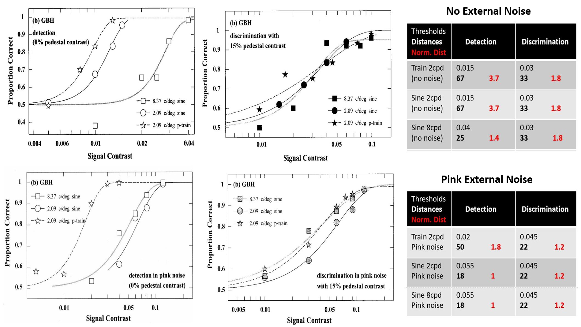
Figure 1: Summary of experimental results by (Henning et al., 2002). (Left) Original psychometric functions for contrast detection and discrimination experiments from one observer, measured with 2.09 and 8.37 cycles per degree (cpd) sinusoidal gratings and 2.09 cpd pulse trains, in the presence and absence of external pink noise. (Right) Thresholds and normalized internal distances in red are the data to be reproduced with the noise-based metric from the pedestal and the incremental test images.

3.2 3.2 Model

In order to illustrate the proposed estimation of the early and late components of the noise we consider the following (simplistic) concatenation of linear and nonlinear layers:

(8)

The input of the model, $\boldsymbol{x}+\boldsymbol{n}^{\varepsilon}$, consist of a stimulus and external noise expressed in $cd/m^{2}$ units. The linear photoreceptors simply add certain early noise (also in luminance units). Following isetbio,Dayan01 we assume a simple Gaussian-Poisson density for the early noise (see Eq. 10 in Appendix A for the expression of the signal-dependent covariance). Clearly, the scaling parameters of this Gaussian-Poisson distribution $\alpha_{e}$ and $\beta_{e}$ are unknown and are the object of our study.

The linear stage applies a set of standard local-oriented filters of different spatial scales [Watson (1987)], and the output of this linear transform is weighted (differentially for each spatial scale) to simulate the effect of the Contrast Sensitivity Function. In particular, we use a steerable wavelet transform [Simoncelli . (1992)] and the method in [Malo . (1997)] to get the optimal CSF weights in that domain. This linear stage can be summarized as the product of two matrices: $\boldsymbol{w}^{\prime}=\mathbb{D}_{\mathrm{CSF}}\cdot W\cdot(\boldsymbol{x}+\boldsymbol{n}^{\varepsilon}+\boldsymbol{n}^{e})$, where $W$ contains the wavelet receptive fields in rows and $\mathbb{D}_{\mathrm{CSF}}$ is a diagonal matrix with the weights that represent the CSF in the diagonal. For the nonlinear stage we take the simplest masking model [Legge  Foley (1980), Legge (1981)]: point-wise saturating functions applied to each coefficient of the linear transform. Specifically, $\boldsymbol{y}=m(\boldsymbol{w}^{\prime})+\boldsymbol{n}^{l}=K\odot\mathrm{sign}(\boldsymbol{w^{\prime}})\odot|\boldsymbol{w}^{\prime}|^{\gamma}+\boldsymbol{n}^{l}$, where following Martinez18, we apply a correction at the origin to avoid singularities in the derivative, and following Martinez19 the constant $K$ is chosen not to modify the relative magnitude of the subbands to preserve the effect of the CSF.

Finally, as for the early noise, the late noise $\boldsymbol{n}^{l}$ is chosen to be Gaussian-Poisson (see covariance in Eq. 10 in Appendix A), and the goal of the proposed method is obtaining the unknowns in the distribution: the scaling parameters $\alpha_{l}$ and $\beta_{l}$.

Again, this simplistic model is far from correct: their elements (e.g. the wavelet transform and the CSF) were just taken off-the-shelf and we just gave reasonable values for its free parameters (the saturation exponent, $\gamma$, and the subband-dependent constant, $K$). Once we estimate the noise for this model using the proposed procedure we will illustrate its reasonable behavior by showing its performance in predicting subjective image quality opinion. However, it is important to stress again that in this work we just wanted a reasonable model good enough to illustrate the method. In this regard, for computational reasons in the optimization, the model has to be easy to compute and with well behaved derivatives, $\nabla S$.

4 4. Results: Noise Estimation

4.1 4.1 Non-parametric Estimation

Our proposal for noise estimation stated in section 2.2 consist of finding the noise parameters that maximize the correlation between $D_{\textrm{exp}}$ (Eq. 5) and $D_{\textrm{theor}}$ (Eq. 7, which depends on the noise). In principle, given $n$ experimental conditions to measure $n$ thresholds, this optimization reduces to computing $\frac{\delta D_{\textrm{theor}}^{i}}{\delta\theta}$, where $\theta$ are the noise parameters and $D_{\textrm{theor}}^{i}$ is the distance for the $i$-th experimental condition, with $i=1,\ldots,n$ [Martinez . (2018)].

However, the inverse in Eq. 7 poses serious computational problems. Note that the derivative of the distance depends on the derivative of the metric, and the inverse implies a dependence on $(\Sigma^{\mathcal{I}})^{-2}$. Computing these inverses of huge matrices in every iteration of the optimization is unfeasible in practice unless strong restrictions in the nature of the noise are assumed.

Therefore, while the parametric expression presented above, Eq. 7, is convenient to understand the problem (for instance to link it to the classical results, or to understand the relevance of the external noise as a scaling factor for the unknowns), in practice, the optimization is easier by taking a nonparametric computation of the theoretical distance. As a result, in order to compute the perceptual distance between $\boldsymbol{x}$ and $\boldsymbol{x}+\Delta\boldsymbol{x}$ from noise, instead of Eq. 7, we propose to take the average Euclidean distance between the noisy responses, $\boldsymbol{y}(\boldsymbol{x})$ and $\boldsymbol{y}(\boldsymbol{x}+\Delta\boldsymbol{x})=\boldsymbol{y}+\Delta\boldsymbol{y}$:

$$D_{\textrm{theor}}^{2} = E\left[\,\Delta\boldsymbol{y}^{\top}\cdot\Delta\boldsymbol{y}\,\right]$$ (9)

$$= E\left[\,\,\,\left|\Delta S+\boldsymbol{n^{\prime}}^{\,\mathcal{I}}-\boldsymbol{n}^{\mathcal{I}}\right|^{2}\,\,\right]$$

where $\Delta S=S(\boldsymbol{x}+\Delta\boldsymbol{x})-S(\boldsymbol{x})$, is the difference between the deterministic responses, and $\boldsymbol{n}^{\mathcal{I}}$ and $\boldsymbol{n^{\prime}}^{\mathcal{I}}$ are realizations of the inner noise at the points $S(\boldsymbol{x})$ and $S(\boldsymbol{x}+\Delta\boldsymbol{x})$ respectively. Note that Eq. 9 means that, when judging the difference between two stimuli, the brain compares two noisy responses: $S(\boldsymbol{x})+\boldsymbol{n}$ and $S(\boldsymbol{x}+\Delta\boldsymbol{x})+\boldsymbol{n^{\prime}}^{\,\mathcal{I}}$

In Appendix C we show the derivatives of the correlation between experimental and theoretical distances with regard to the noise parameters from Eq. 9. In this non-parametric case, the derivatives wrt noise do not involve matrix inversion, and hence they are easy to compute. This allows a practical optimization of the noise parameters (no matter the complexity of the noise) whenever $\nabla S$ is easy to compute.

Eq. 9 also implies the relevance of input (external and early noise) as a scale factor for the late noise. However, this relevance is not that obvious in this expression because it is hidden in the distribution of the samples of the inner noise $\boldsymbol{n}^{\mathcal{I}}$. The relevance can be seen analytically in this particular case: if the inner noise distributions are symmetric -zero skewness- (which is reasonable under mild nonlinearities) and we impose zero distance for $\Delta\boldsymbol{x}=0$ (which is an obvious linear recalibration of the distance), in Appendix D we show that Eq. 9 reduces to $D_{\textrm{theor}}^{2}=|\Delta S|^{2}+|\boldsymbol{n}^{\prime\mathcal{I}}|^{2}-|\boldsymbol{n}^{\mathcal{I}}|^{2}$. In that case, as the realizations of the inner noise depend on the late noise and on the input noise, we have: $\boldsymbol{n}^{\mathcal{I}}=\boldsymbol{n}^{l}(S(\boldsymbol{x}))+\nabla S\cdot\boldsymbol{n}^{\varepsilon e}+\boldsymbol{n}^{l}(\nabla S\cdot\boldsymbol{n}^{\varepsilon e})$. Therefore, for a fixed difference in response, $\Delta S$, the interesting (anisotropic) behavior of the distance in different directions comes from the anisotropy of the noise. If there is no input noise (i.e. $\boldsymbol{n}^{\varepsilon e}=0$) then one could scale the late noise by an arbitrary factor $k$ and get the same anisotropy. Therefore, this scaling factor would have no effect in the correlation, and hence the global scale of the late noise would be arbitrary. This is easily avoided by using some external non-spherical noise, for instance pink noise as in [Henning . (2002)], in the experiments.

On top of the observation of the relevance of external and early noise also in Eq. 9, Appendix D shows the equivalence in the anisotropy found through the parametric distance, Eq. 7, and the non parametric distance Eq. 9, which has more convenient derivatives.

As a consequence, for computational convenience, we chose this specific non-parametric definition to get the parameters of the noise.

4.2 4.2 Results

Using the data and model considered in Section 3 and the computationally convenient noise-dependent distance described in Eq. 9 and Appendix D, we looked for the noise parameters that maximize the correlation between theory and experiment.

In our case we assumed Gaussian-Poisson noise applied independently to every photodetector (early noise) and to every sensor at the saturated wavelet representation (late noise). The corresponding covariances of the noise are given in Appendix A. These covariances were used to generate noisy inputs and responses in the non-parametric computation of the distances. We used ADAM optimization using the derivatives of the distance reported in Appendix C.

Fig. 2 shows two illustrative results of such procedure. We used all the experimental detection and discrimination data using pulse-trains and sinusoids of different frequencies in external pink noise and with no external noise.

The top panel shows the results for the Gaussian-Poisson case and the bottom panel shows the equivalent result when the noises are assumed to be purely Poisson (with no Gaussian component, and hence $\alpha_{e}=\alpha_{l}=0$).

Each panel shows the scatter plot at the left with the number of iterations in the optimization and the achieved correlation. The iteration stopped when the improvement in the correlation was negligible. The plots at the right show the evolution of the correlation during the optimization and the evolution of the noise parameters. The numbers show the results for the standard deviation $\alpha$ and the fano factor $\beta$ of the noises.

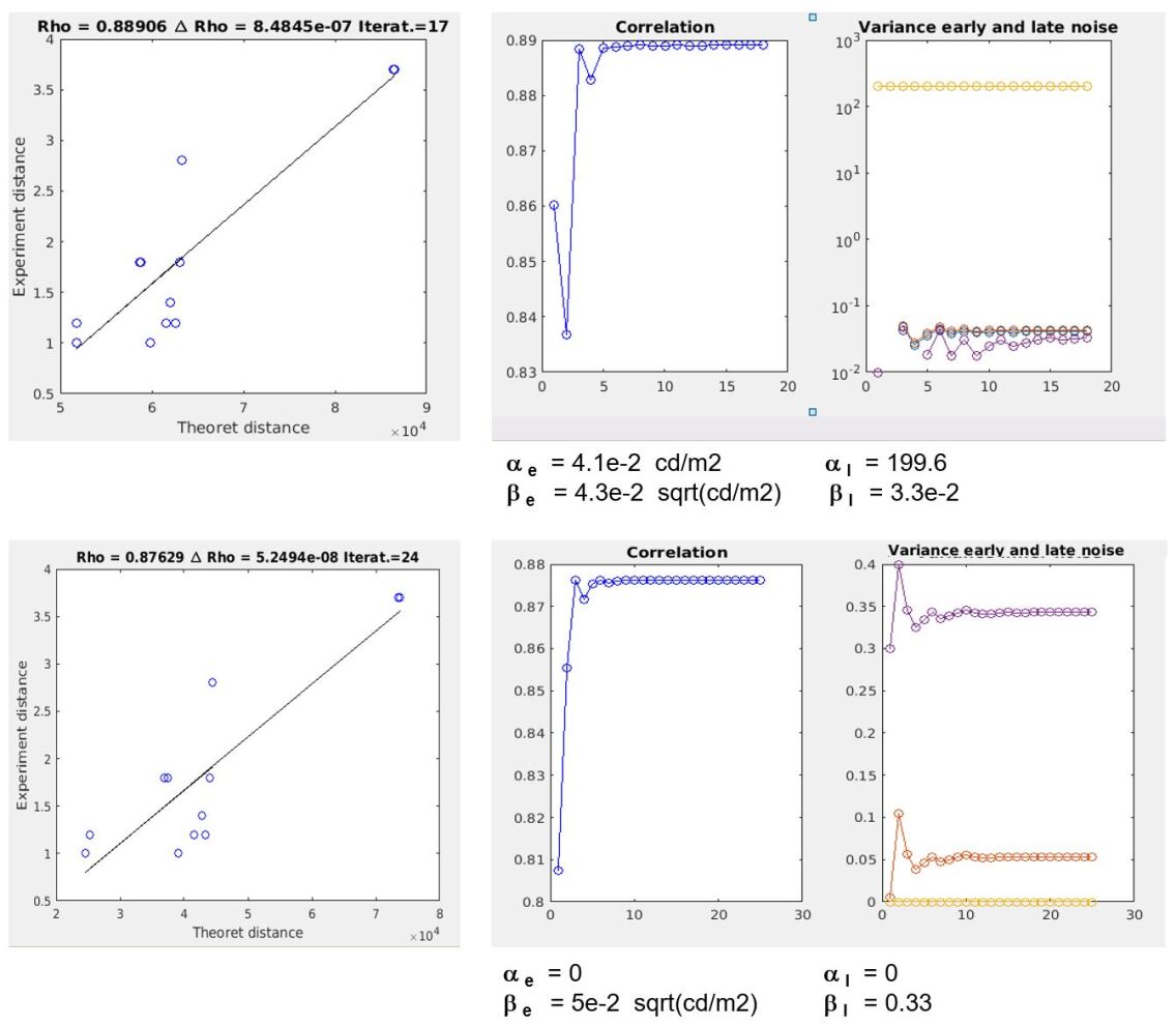
Figure 2: Early and late noise parameters from the maximization of the correlation between theory and data on detection and discrimination in external pink noise.

Appendix E checks the consistency of these results in two different ways. First, from the technical point of view, we show that if data with no external noise are considered and no early noise is assumed either, the result of the late noise is indeed underdetermined, thus confirming the comments we made on Eqs. 7 and 9. Second, we show that the considered model together with the noise estimate makes a reasonable job in predicting subjective distances in a totally different (suprathreshold) application.

5 5. Discussion

5.1 5.1 Psychophysical versus Physiological estimates

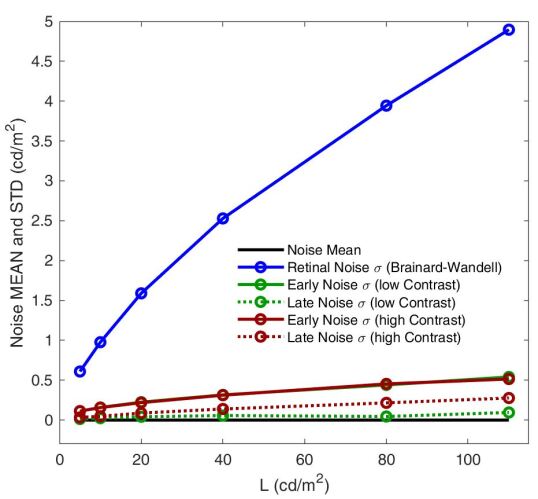
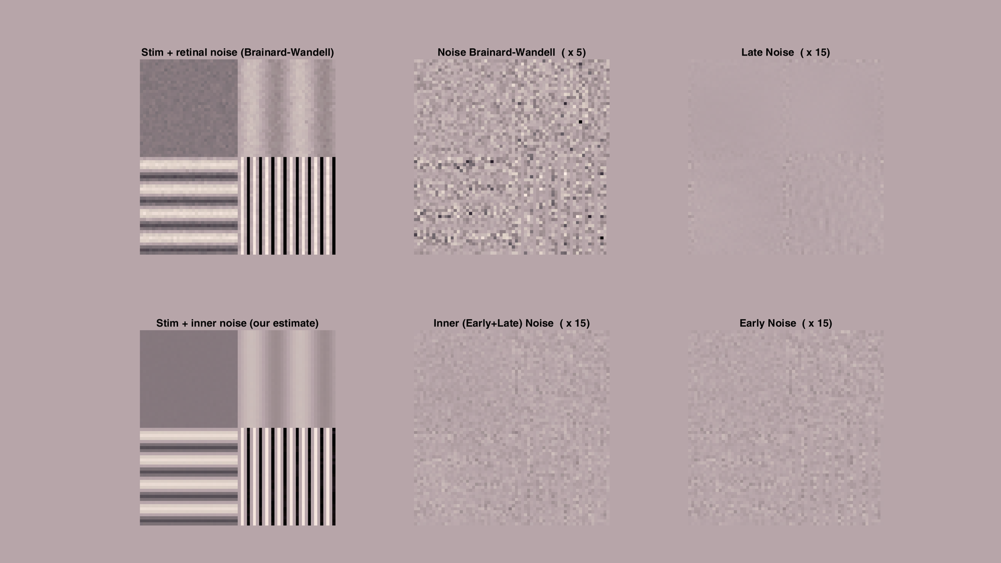
Figure 3: Comparison of the physiological (retinal) noise estimation according to (Brainard & Wandell, 2020), and the psychophysical (Early and Late) estimations proposed here. Top panel: shows the standard deviation of the early and the late noises as a function of the luminance and contrast of the (sinusoidal) stimulus. As expected by the Weber-law and contrast masking, the noise increases with luminance and with contrast. The std of the physiological noise in the retina is plotted in the same units as a reference. Bottom panel: shows a representative stimulus calibrated in luminance with the inner noise of both models inverted back into the image space. Luminance of the flat square is 35 $cd/m^{2}$. Average luminance of the sinusoids is 70 $cd/m^{2}$. Frequencies are 2, 4 and 8 cpd, and contrasts are 0.3, 0.8, and 1 respectively.

Our psychophysical estimates of the noise should be reasonable, that is within realistic bounds set by physiological measurements. Naïvely, one might think that our psychophysical estimate of the early noise should be directly related to the noise in the electrical response of L,M,S retinal cones. Similarly, one may think that our late noise could be related to the noise within the first cortical visual areas. However, here we show that direct comparison is not that simple—as always it is non-trivial to relate properties of single neurons to the behaviour of the organism in its entirety.

Appendix F describes how we used ISETBIO [Brainard  Wandell (2020)] to obtain physiological estimation of retinal noise. The discussion to follow will clarify why the comparison is not straightforward and why we argue that it is sensible to have one order of magnitude less noise in a psychophysical model which does not take eye movements into account.

Fig. 3 (top panel) shows the standard deviation of our estimated early and late noise sources on top of a low-contrast sinusoid for different average luminances. The equivalent ISETBIO noise estimate in $cd/m^{2}$ is plotted on top for useful reference. Fig. 3 (bottom panel) shows sample images with ISETBIO noise estimate and with the inner noise estimated by us, both back in the spatial domain. If noise controls the discriminability, it should be just noticeable (or barely visible) for the average observer. Clearly, that is not the case for the physiological noise in the retina as estimated using ISETBIO. To us this indicates the presence of down-stream mechanisms to remove the noise, e.g. via motion compensation, evidence accumulation over time or spatial low-pass filtering. Conversely, our psychophysically obtained noise estimate is almost invisible on top of the background pattern. In order to explore its nature and assess its early/late components we show scaled versions of the noises on top of a flat background of 70 $cd/m^{2}$. Whilst the Poisson early noise (trivially) inherits the spatial structure of the luminance, the late noise also displays a contrast and frequency dependence due to the inner working of the nonlinear wavelet filters of the deterministic model.

5.2 5.2 Experimental consequences: Maximum Differentiation from noise estimates

The proposed method to disentangle external, early and late noise gives an unprecedented experimental tool to decide between psychophysical models. The concept of Maximum Differentiation has been proposed as a way to decide between vision models [Wang  Simoncelli (2008)], or as a way to measure the free parameters of vision models [Malo  Simoncelli (2015)] using the associated perceptual distance.

Originally [Wang  Simoncelli (2008)] proposed a method to generate stimuli maximally/minimally discernible by observers according to an iterative procedure of perceptual distance maximization/minimization. This, depending of the model may be extremely expensive. However, following the second order approximation of the non-Euclidean distance used in Appendix A [Epifanio . (2003), Malo  Simoncelli (2006)], we proposed a simplification of the Maximum Differentiation method based on estimating the eigenvectors of the discrimination ellipsoid [Malo  Simoncelli (2015), Martinez . (2018)].

The theory proposed here allows the estimation of the covariance matrix of the inner noise and hence the design of interesting stimuli in cardinal directions of the noise-dependent metric.

Fig. 4 illustrates the potential of the external vs intrinsic noise of the system to design noise-related Maximum Differentiation stimuli. There we use a toy model acting on 2-pixel images with certain inner noise (red ellipses) together with some pink noise used by the experimenter (blue ellipses) at different points (images) of the image space. Taking into account that the usual linear+nonlinear operations in the conventional vision models are just affine rotations/deformations (implemented by sensors tuned to different spatial frequencies) and nonlinear rescaling of the axes (sensor saturation), we get transforms of the domain such as the one illustrated in the figure.

Propagation of the noise-related discrimination ellipsoids in this example (that in reality could be estimated with the technique proposed here) show how certain external noise may dominate discrimination at some places of the domain but not in others. And these facts could be checked through Maximum Differentiation using the eigenvectors of the corresponding ellipsoids.

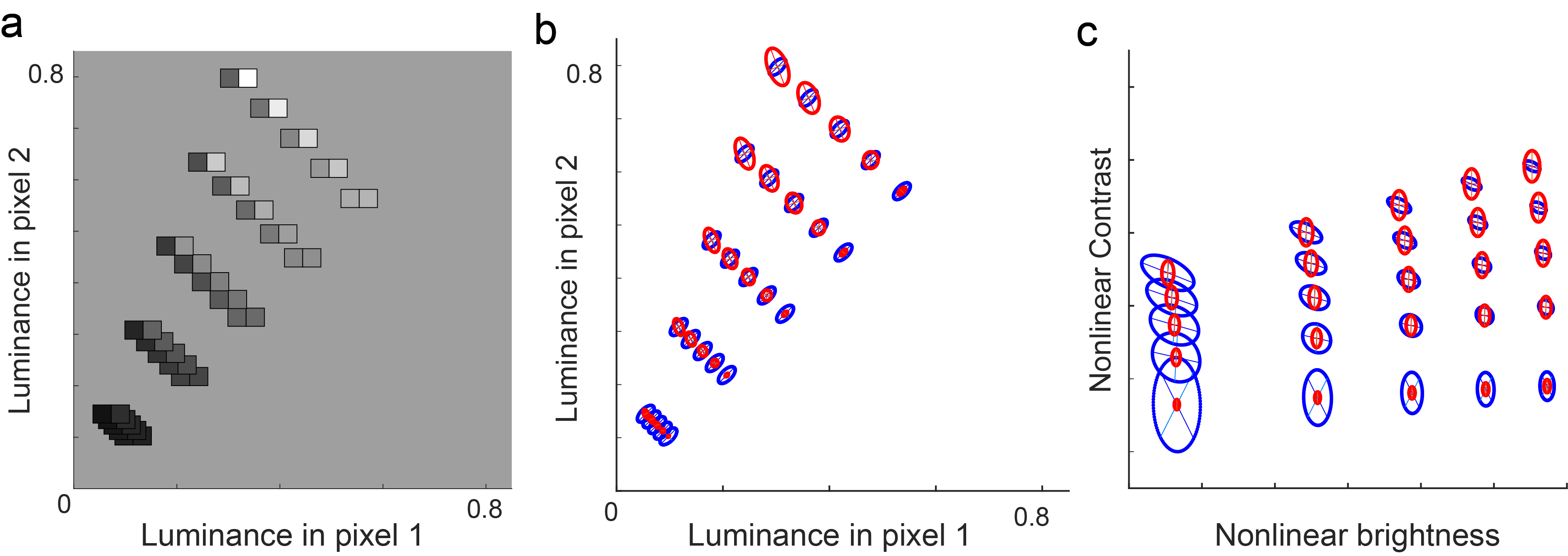
Figure 4: Discrimination predictions in a 2-dimensional toy model example. (a) The stimulus space in the toy model consists of only two pixels varying in luminance. The added external noise at the input space (blue ellipses, b) gets propagated through the model up to the internal representation space (c), at which late noise is added (red ellipses in c). Given a model and the noise covariance estimation, we can compute the directions of better and worse discrimination.

5.3 5.3 Final remarks

The estimated variance of the early and late noise can be used for a more accurate account of the mutual information between the retinal image and the inner representation. With the proposed method realistic values for the noise could be obtained for any model, and hence the results in [Malo (2020)] on the information transmitted by spatial vs chromatic mechanisms or by linear vs nonlinear transforms could be more than rough estimates with reasonable noise assumptions. Similarly, better noise estimates could lead to an improvement of image quality measures such as [Sheikh  Bovik (2006)] based on modeling information transference along the visual pathway.

The proposed late-noise estimation procedure from experiments using early-noise may be used to modify the (inner noise or inner metric) assumptions in recent models of spatial vision [Schutt  Wichmann (2017), Martinez . (2018)], as well as to solve debates on the relative relevance of the noise and the nonlinearities of the models [Georgeson  Meese (2006)].

6 Appendix A: Derivation of Eq. 7 (general and particular cases)

General case Demo in pages 9-11 of the googledoc. Result listed in page 2 of progress_conventional.pdf (mail sept. 23rd).

Particular case: Gauss-Poisson if early and late noise are Gaussian-Poisson variables:

$$\Sigma^{e}(\boldsymbol{x}) = \alpha_{e}^{2}I+\beta_{e}^{2}\,\mathbb{D}_{|\boldsymbol{x}|}+2\alpha_{e}\beta_{e}\,\mathbb{D}_{|\boldsymbol{x}|^{1/2}}$$ (10)

$$\Sigma^{l}(S(\boldsymbol{x})) = \alpha_{l}^{2}I+\beta_{l}^{2}\,\mathbb{D}_{|S(\boldsymbol{x})|}+2\alpha_{l}\beta_{l}\,\mathbb{D}_{|S(\boldsymbol{x})|^{1/2}}$$

Therefore, the noise at the input for certain stimulus $\boldsymbol{x}$, in the Gaussian-Poisson case is:

$$\Sigma^{\varepsilon e} = k_{e}\Sigma^{e}+\underbrace{\Sigma^{\varepsilon}+k_{e}\frac{\beta_{e}^{2}}{4}\,\mathbb{D}_{|\boldsymbol{x}|^{-1/2}}\cdot\Sigma^{\varepsilon}\cdot\mathbb{D}_{|\boldsymbol{x}|^{-1/2}}}_{\textit{external noise}}$$ (11)

$$= k_{e}\Sigma^{e}+\underbrace{\Sigma^{\varepsilon}+M(\Sigma^{\varepsilon})}_{\textit{external noise}}$$

7 Appendix B: Burgess & Colborne 88 as a special case of Eq. 7

Our general expression reduces to the classical result in [Burgess  Colborne (1988)] in this (very restricted) case: linear systems with no early noise, stationary external noise, and stationary-signal-independent late noise.

Demo in page 36 of googledoc.

8 Appendix C: Optimization of correlation from Eq. 9

Demo of derivatives in page 15 of googledoc. Derivatives checked numerically in these files (and folder):

• deriv_response_wrt_param_numeric_analytic_3_pixels.m

• deriv_difference_wrt_noise_actual_scale.m

• Folder: /media/disk/vista/Papers/A_GermanyValencia/NOISE_and_MAD/...
.../simple_model/check_deriv_distance/

These results are listed in page 3 of progress_conventional.pdf (mail sept. 23rd).

Note: those analytical results can be further simplified if we take the average value. I will do when I transcribe here. That may speed up the derivatives even more!.

9 Appendix D: Equivalence of parametric and non-parametric distances

In this appendix we show that the considered distances are equally valid to get the corresponding estimation of the noise. First we show that the distances have an interesting anisotropic behavior depending on the noise: perceptual distance is markedly different for distortions in different directions $\Delta\boldsymbol{x}$. The noise-dependent anisotropy is obvious in Eq. 7 because the metric depends on the covariance of the noise, but this is less obvious in the non-parametric Eq. 9.

The first part of this Appendix analytically shows that the non-parametric distance displays this anisotropy. Afterwards, we numerically show that the distance computed in both ways can be linearly related. As a result, since correlation is independent of a linear transformation applied to one of the axis, both definitions of $D_{\textrm{theor}}$ are equivalent for our purposes.

Analytical part: nonparametric distance is anisotropic. Demo in page 37 of googledoc and illustrated numerically in
toy_non_parametric_2.m

In the main text we said that Eq. 9 displays a non-isotropic behavior depending on the distribution of the inner noise. In order to make this more evident, one should start from the obvious re-calibration of the distance: first ensure that the distance is zero when $\Delta S=0$. In order to do that one has to subtract the energy of the inner noise for $\boldsymbol{x}$ in order to get zero distance when $\Delta\boldsymbol{x}$ (and $\Delta S$) are zero. Then, see demo in page 37 of googledoc.

Numerical part: non-parametric and parametric anisotropies are linearly related This was empirically checked in our 2D vision model (see toy_example_2.zip, and distance_sampling_vs_parametric.m (sent by mail 14 oct. 2020, described in the document progressconventional2.pdf, and in the 30th sept entry in googledoc (page 28).)

10 Appendix E: Consistency of results

10.1 E.1 No early noise implies indetermination of the variance

Figure 5 shows the correlation in explaining discrimination and detection data in negligible early noise condition when different factors are applied to the optimum values obtained form a zero initialization. This illustrates the indetermination in the variance pointed out in discussing eq. 7.

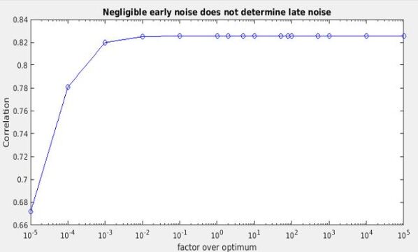
Figure 5: Indetermination of variance. Once the level of noise reaches the threshold defined by the (arbitrarily small) early noise introduced to avoid singularities at zero, the late noise value may be multiplied by an arbitrary factor bigger than 1 and no effect is obtained in the correlation.

As anticipated in discussing the expression, this implies that measurements with substantial early noise are required to solve this indetermination.

10.2 E.2 Our noise estimate together with the considered model predict image quality

Our (off-the-shelf, non-optimized) deterministic model equipped with our early/late noise estimates does a reasonable job in predicting image quality. See Fig. 6

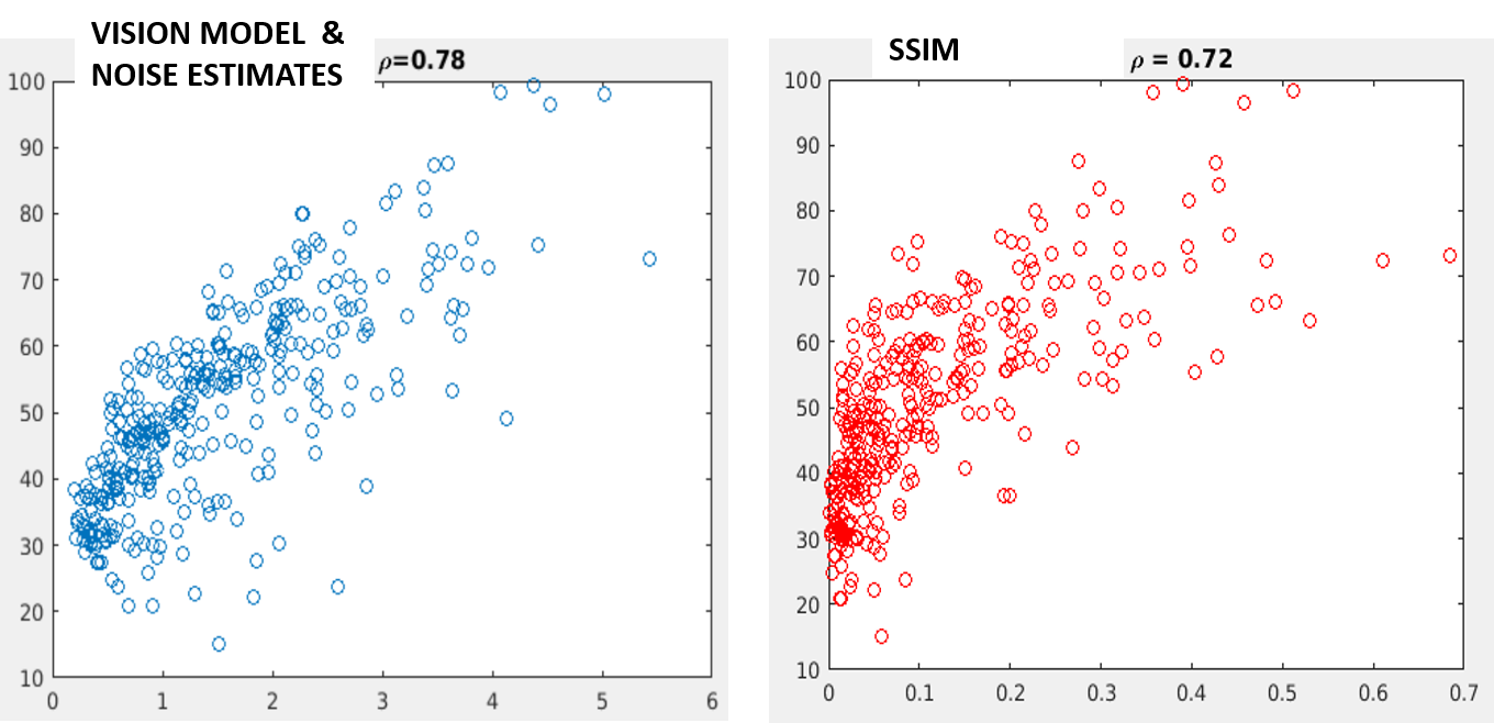
Figure 6: Prediction of subjective image quality using the noise estimates (left) and SSIM (right). Subjective distances of TID database (experimental distance in ordinates) versus the distance $D_{\textrm{theor}}$ in abscissas. Correlation with human opinion is substantially better using a simple model and our noise estimations ($\rho_{\textrm{noise}}=0.78$) than the obtained by widely used subjective quality metrics like SSIM ($\rho_{\textrm{SSIM}}=0.72$). This suggests the applicability of our noise estimations in suprathreshold conditions.

We did this in images_TID_atd_through_simple_model.m and gather_small_results_TID_color.m (in HAL folder /media/disk/vista/Papers/A_GermanyValencia/NOISE_and_MAD/simple_model/check_on_TID

11 Appendix F: Physiological estimates of early noise using ISETBIO

Here we described how we used ISETBIO [Brainard  Wandell (2020)] to get a reasonable physiological estimation of retinal noise, which, in principle, would be the physiological correlate of our psychophysical early noise estimate. The discussion clarifies why the comparison is not straightforward and why it is sensible to have one order of magnitude less noise in a psychophysical model which doesnt take eye movements into account.

Fig. 7 shows the procedure we followed for the physiological estimation of the noise in (comparable) $cd/m^{2}$ units.

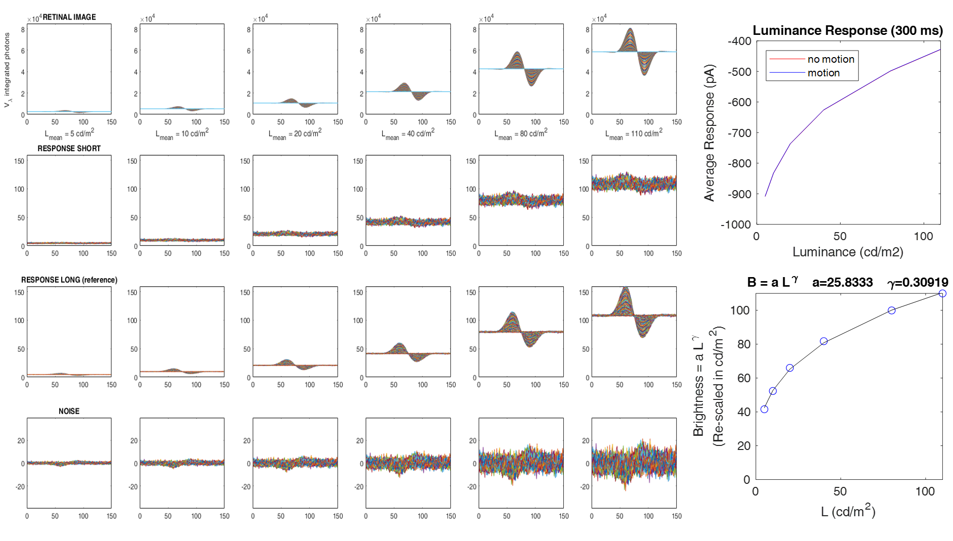
Figure 7: Photocurrent noise expressed in luminance units ($cd/m^{2}$) using simulations of ISETBIO for different average luminances of the test pattern and fitting a conventional photocurrent (brightness) vs luminance exponential function.

Here I will include the explanations given in noise_in_ISETBIO.pdf (mail) 29 oct 2020, and in
OUR_noise_and_ISETBIO.pdf (mail 18 nov. 2020) and computed through estimate_noise_3.m

References

- Ahumada (\APACyear1987) \APACinsertmetastarAhumada87Ahumada, A\BPBIJ. \APACrefYearMonthDay1987Dec. \BBOQ\APACrefatitlePutting the visual system noise back in the picturePutting the visual system noise back in the picture.\BBCQ \APACjournalVolNumPagesJ. Opt. Soc. Am. A4122372–2378. {APACrefURL} http://josaa.osa.org/abstract.cfm?URI=josaa-4-12-2372 , doi:10.1364/JOSAA.4.002372 \PrintBackRefs\CurrentBib
- Bracewell (\APACyear1986) \APACinsertmetastarBracewell_1986Bracewell, R\BPBIN. \APACrefYearMonthDay1986\APACmonth01. \BBOQ\APACrefatitleThe Fourier Transform and its ApplicationsThe Fourier Transform and its Applications.\BBCQ \PrintBackRefs\CurrentBib
- Brainard \BBA Wandell (\APACyear2020) \APACinsertmetastarisetbioBrainard, D.\BCBT \BBA Wandell, B. \APACrefYearMonthDay2020Nov.. \BBOQ\APACrefatitleISETBIO: tools for modeling the human visual system front endIsetbio: tools for modeling the human visual system front end\BBCQ [\bibcomputersoftwaremanual]. \PrintBackRefs\CurrentBib
- Burgess \BBA Colborne (\APACyear1988) \APACinsertmetastarBurgess88Burgess, A.\BCBT \BBA Colborne, B. \APACrefYearMonthDay1988April. \BBOQ\APACrefatitleVisual signal detection, IV: Observer inconsistency.Visual signal detection, IV: Observer inconsistency.\BBCQ \APACjournalVolNumPagesJOSA A54617–627. \PrintBackRefs\CurrentBib
- Campbell \BBA Robson (\APACyear1968) \APACinsertmetastarCampbell_1968Campbell, F\BPBIW.\BCBT \BBA Robson, J\BPBIG. \APACrefYearMonthDay1968. \BBOQ\APACrefatitleApplication of fourier analysis to the visibility of gratingsApplication of fourier analysis to the visibility of gratings.\BBCQ \APACjournalVolNumPagesThe Journal of Physiology1973551–566. \PrintBackRefs\CurrentBib
- Dayan \BBA Abbott (\APACyear2005) \APACinsertmetastarDayan01Dayan, P.\BCBT \BBA Abbott, L\BPBIF. \APACrefYear2005. \APACrefbtitleTheoretical Neuroscience: Computational and Mathematical Modeling of Neural SystemsTheoretical neuroscience: Computational and mathematical modeling of neural systems. \APACaddressPublisherThe MIT Press. \PrintBackRefs\CurrentBib
- Epifanio \BOthers. (\APACyear2003) \APACinsertmetastarEpifanio03Epifanio, I., Gutierrez, J.\BCBL \BBA Malo, J. \APACrefYearMonthDay2003. \BBOQ\APACrefatitleLinear transform for simultaneous diagonalization of covariance and perceptual metric matrix in image codingLinear transform for simultaneous diagonalization of covariance and perceptual metric matrix in image coding.\BBCQ \APACjournalVolNumPagesPatt. Recog.3681799–1811. \PrintBackRefs\CurrentBib
- Georgeson \BBA Meese (\APACyear2006) \APACinsertmetastarMesse06Georgeson, M.\BCBT \BBA Meese, T. \APACrefYearMonthDay2006. \BBOQ\APACrefatitleFixed or variable noise in contrast discrim.? The jury’s still outFixed or variable noise in contrast discrim.? the jury’s still out.\BBCQ \APACjournalVolNumPagesVis.Res.46254294–4303. \PrintBackRefs\CurrentBib
- Henning \BOthers. (\APACyear2002) \APACinsertmetastarWichmann02Henning, G., Bird, C.\BCBL \BBA Wichmann, F. \APACrefYearMonthDay2002Jul. \BBOQ\APACrefatitleContrast discrimination of pulse trains in pink noiseContrast discrimination of pulse trains in pink noise.\BBCQ \APACjournalVolNumPagesJOSA A1971259–1266. {APACrefURL} http://josaa.osa.org/abstract.cfm?URI=josaa-19-7-1259 , doi:10.1364/JOSAA.19.001259 \PrintBackRefs\CurrentBib
- Laparra \BOthers. (\APACyear2010) \APACinsertmetastarLaparra10aLaparra, V., Muñoz, J.\BCBL \BBA Malo, J. \APACrefYearMonthDay2010. \BBOQ\APACrefatitleDivisive normalization image quality metric revisitedDivisive normalization image quality metric revisited.\BBCQ \APACjournalVolNumPagesJOSA A274852–864. \PrintBackRefs\CurrentBib
- Legge (\APACyear1981) \APACinsertmetastarLegge81Legge, G. \APACrefYearMonthDay1981. \BBOQ\APACrefatitleA Power Law for Contrast DiscriminationA power law for contrast discrimination.\BBCQ \APACjournalVolNumPagesVision Research1868–91. \PrintBackRefs\CurrentBib
- Legge \BBA Foley (\APACyear1980) \APACinsertmetastarLegge80Legge, G.\BCBT \BBA Foley, J. \APACrefYearMonthDay1980. \BBOQ\APACrefatitleContrast Masking in Human VisionContrast masking in human vision.\BBCQ \APACjournalVolNumPagesJournal of the Optical Society of America701458–1471. \PrintBackRefs\CurrentBib
- Mahalanobis (\APACyear1936) \APACinsertmetastarMaha36Mahalanobis, P. \APACrefYearMonthDay1936. \BBOQ\APACrefatitleOn the generalized distance in statisticsOn the generalized distance in statistics.\BBCQ \APACjournalVolNumPagesProc. Nat. Inst. Sci. India2149–55. \PrintBackRefs\CurrentBib
- Malo (\APACyear2020) \APACinsertmetastarMalo20Malo, J. \APACrefYearMonthDay2020. \BBOQ\APACrefatitleSpatio-chromatic information available from different neural layers via GaussianizationSpatio-chromatic information available from different neural layers via gaussianization.\BBCQ \APACjournalVolNumPagesJ. Math. Neurosci.1018. , doi:10.1186/s13408-020-00095-8 \PrintBackRefs\CurrentBib
- Malo \BOthers. (\APACyear1997) \APACinsertmetastarMalo97Malo, J., Pons, A., Felipe, A.\BCBL \BBA Artigas, J. \APACrefYearMonthDay1997. \BBOQ\APACrefatitleCharacterization of the human visual system threshold performance by a weighting function in the Gabor domainCharacterization of the human visual system threshold performance by a weighting function in the gabor domain.\BBCQ \APACjournalVolNumPagesJournal of Modern Optics441127-148. \PrintBackRefs\CurrentBib
- Malo \BBA Simoncelli (\APACyear2006) \APACinsertmetastarMalo06aMalo, J.\BCBT \BBA Simoncelli, E. \APACrefYearMonthDay2006. \BBOQ\APACrefatitleNonlinear image representation for efficient perceptual codingNonlinear image representation for efficient perceptual coding.\BBCQ \APACjournalVolNumPagesIEEE Trans.Im.Proc.15168–80. \PrintBackRefs\CurrentBib
- Malo \BBA Simoncelli (\APACyear2015) \APACinsertmetastarMalo15Malo, J.\BCBT \BBA Simoncelli, E. \APACrefYearMonthDay2015. \BBOQ\APACrefatitleGeometrical and statistical properties of vision models obtained via maximum differentiationGeometrical and statistical properties of vision models obtained via maximum differentiation.\BBCQ \BIn \APACrefbtitleProc. SPIE Electronic ImagingProc. SPIE Electronic Imaging (\BPGS 93940L–93940L). \PrintBackRefs\CurrentBib
- Martinez \BOthers. (\APACyear2018) \APACinsertmetastarMartinez18Martinez, M., Bertalmío, M.\BCBL \BBA Malo, J. \APACrefYearMonthDay2018. \BBOQ\APACrefatitleDerivatives and Inverse of Cascaded L+NL Neural ModelsDerivatives and inverse of cascaded L+NL neural models.\BBCQ \APACjournalVolNumPagesPLoS 13(10):e0201326. \PrintBackRefs\CurrentBib
- Martinez \BOthers. (\APACyear2019) \APACinsertmetastarMartinez19Martinez, M., Bertalmío, M.\BCBL \BBA Malo, J. \APACrefYearMonthDay2019. \BBOQ\APACrefatitleIn Praise of Artifice Reloaded: Caution with Natural Image Databases in Modeling VisionIn praise of artifice reloaded: Caution with natural image databases in modeling vision.\BBCQ \APACjournalVolNumPagesFront. Neurosci. doi: 10.3389/fnins.2019.00008. , doi:doi: 10.3389/fnins.2019.00008 \PrintBackRefs\CurrentBib
- Schutt \BBA Wichmann (\APACyear2017) \APACinsertmetastarWichmann17Schutt, H.\BCBT \BBA Wichmann, F. \APACrefYearMonthDay2017. \BBOQ\APACrefatitleAn image-computable psychophysical spatial vision modelAn image-computable psychophysical spatial vision model.\BBCQ \APACjournalVolNumPagesJ. Vision171212. \PrintBackRefs\CurrentBib
- Sheikh \BBA Bovik (\APACyear2006) \APACinsertmetastarSheikh06Sheikh, H\BPBIR.\BCBT \BBA Bovik, A\BPBIC. \APACrefYearMonthDay2006\APACmonth02. \BBOQ\APACrefatitleImage Information and Visual QualityImage information and visual quality.\BBCQ \APACjournalVolNumPagesIEEE Trans. Img. Proc.152430–444. {APACrefURL} http://dx.doi.org/10.1109/TIP.2005.859378 , doi:10.1109/TIP.2005.859378 \PrintBackRefs\CurrentBib
- Simoncelli \BOthers. (\APACyear1992) \APACinsertmetastarSimoncelli92Simoncelli, E\BPBIP., Freeman, W\BPBIT., Adelson, E\BPBIH.\BCBL \BBA Heeger, D\BPBIJ. \APACrefYearMonthDay1992Mar. \BBOQ\APACrefatitleShiftable multi-scale transformsShiftable multi-scale transforms.\BBCQ \APACjournalVolNumPagesIEEE Trans Information Theory382587–607. \APACrefnoteSpecial Issue on Wavelets , doi:10.1109/18.119725 \PrintBackRefs\CurrentBib
- Wang \BBA Simoncelli (\APACyear2008) \APACinsertmetastarWang08Wang, Z.\BCBT \BBA Simoncelli, E\BPBIP. \APACrefYearMonthDay2008. \BBOQ\APACrefatitleMaximum differentiation (MAD) competition: A methodology for comparing computational models of perceptual quantitiesMaximum differentiation (MAD) competition: A methodology for comparing computational models of perceptual quantities.\BBCQ \APACjournalVolNumPagesJournal of Vision8128–8. \PrintBackRefs\CurrentBib
- Watson (\APACyear1987) \APACinsertmetastarWatson87bWatson, A. \APACrefYearMonthDay1987. \BBOQ\APACrefatitleThe Cortex Transform: Rapid Computation of Simulated Neural ImagesThe cortex transform: Rapid computation of simulated neural images.\BBCQ \APACjournalVolNumPagesComputer Vision, Graphics and Image Processing39311–327. \PrintBackRefs\CurrentBib
- Wichmann (\APACyear1999) \APACinsertmetastarWichmann_1999Wichmann, F. \APACrefYear1999. \APACrefbtitleSome Aspects of Modelling Human Spatial Vision: Contrast DiscriminationSome aspects of modelling human spatial vision: Contrast discrimination. \BUPhD, Univ. of Oxford. \PrintBackRefs\CurrentBib