Parallel Software to Offset the Cost of Higher Precision

Abstract

Hardware double precision is often insufficient to solve large scientific problems accurately. Computing in higher precision defined by software causes significant computational overhead. The application of parallel algorithms compensates for this overhead. Newton’s method to develop power series expansions of algebraic space curves is the use case for this application.

1. Problem Statement and Overview

While parallel computers are fast and can solve large problems, the propagation of roundoff errors increases as problems grow larger and the hardware supports only double precision. If we can afford the same time as on a sequential run, then we ask for quality up: by how much can we improve the quality of the results with a parallel run? To us, quality means accuracy. The goal is to compensate for the overhead of multiple double arithmetic with parallel computations.

The focus of this paper is on recently developed code for new algorithms described in [3], [12, 13], added to PHCpack [14]. PHCpack is a free and open source package to apply Polynomial Homotopy Continuation to solve systems of many polynomials in several variables. Continuation methods are classic algorithms in applied mathematics, see e.g. [9]. Ada is the main language in which the algorithms in PHCpack have been developed during the past thirty years. Strong typing and standardization make that the same code runs on different platforms (Linux, Windows, Mac OS X) and that the same code continues to run, even after decades, without the need to update for upgrades of the language. Ada tasking provides an effective high level tool to develop algorithms for parallel shared memory computers; see [2] or [8] for introductions.

Using QDlib [6] and the software CAMPARY [7], we extend the range of precision offered by hardware doubles [10], as a step towards rigorous verification. In our numerical study of algebraic curves [15], we apply algorithmic differentiation [5], numerical linear algebra [4], and rational approximation techniques [1].

The first three sections in this paper motivate the need for higher precision and describe the computational cost overhead. This overhead then motivates the application of multitasking. All computational experiments for this paper were done on a CentOS Linux workstation with 256 GB RAM and two 22-core 2.2 GHz Intel Xeon E5-2699 processors.

2. Multiple Double Numbers

A double double is an unevaluated sum of two hardware doubles. With the application of basic arithmetical operations in IEEE double format, we obtain more accurate results, up to twice the accuracy of the hardware double precision. In [11], double double arithmetic is described in the context of error-free transformations; see also [10, Chapter 14]. Double double and quad double arithmetic is provided by QDlib [6]. Code generators for general multiple double and multiple float arithmetical operations are available in the software CAMPARY [7].

As an illustration of multiple double arithmetic, consider the computation of the 2-norm of a vectors of dimension 64 of complex numbers generated as $\cos(\theta)+\sin(\theta)\sqrt{-1}$, for random angles $\theta$. The 2-norm equals 8. Observe the second double of the multiple double 2-norm.

      double double : 8.00000000000000E+00 - 6.47112461314111E-32
      triple double : 8.00000000000000E+00 + 1.78941597340672E-48
        quad double : 8.00000000000000E+00 + 3.20475411419393E-65
       penta double : 8.00000000000000E+00 + 2.24021706293649E-81
        octo double : 8.00000000000000E+00 - 9.72609915198313E-129
        deca double : 8.00000000000000E+00 + 3.05130075600701E-161

The format of the result above is for this experiment preferable over the decimal expansion which may appear as $7.999\ldots 9$. The Ada code for multiple double precision is available in the free and open source software PHCpack [14], under version control at github.

Table 1 shows the cost of the basic operations in multiple double precision, expressed in the number of hardware double arithmetical operations. A tenfold increase in precision from double to deca double leads to a more than thousandfold increase in the count of the arithmetical operations.

	double double				triple double				quad double
	$+$	$-$	$*$	$/$	$+$	$-$	$*$	$/$	$+$	$-$	$*$	$/$
add	8	12			13	22			35	54
mul	5	9	9		83	84	42		99	164	73
div	33	18	16	3	113	214	63	4	266	510	112	5
	penta double				octo double				deca double
	$+$	$-$	$*$	$/$	$+$	$-$	$*$	$/$	$+$	$-$	$*$	$/$
add	44	78			95	174			139	258
mul	162	283	109		529	954	259		952	1743	394
div	474	898	175	6	1599	3070	448	9	2899	5598	700	11

Table 1: Number of double operations for addition (add), multiplication (mul), division (div), required for a 2-fold, 3-fold, 4-fold, 5-fold, 8-fold, and 10-fold increase in precision.

The operation counts in Table 1 then motivate the need for parallel computations as follows. What takes a millisecond to compute in double precision will take several seconds in deca double precision. A program that finishes in a second in double precision will take more than an hour in deca double precision. A computation in double precision that takes a hour will in deca double precision take more than a month to finish.

3. Polynomials as Truncated Power Series

Writing a polynomial backwards (starting at the constant term and then listing the monomials in the increasing degree order), leads to the interpretation of a polynomial as the sum of the leading terms in a power series. Unlike polynomials, every power series with a leading nonzero constant term has an inverse. One can divide power series by another and calculate with power series similar as to number arithmetic [15]. In this section, we consider Newton’s method where the arithmetic happens with truncated power series instead of with ordinary numbers.

One common parameter representation for points on the circle with radius one is $(\cos(t),\sin(t))$, for $t\in[0,2\pi[$. With truncated power series arithmetic we can approximate this representation. Consider a system of two polynomials in three variables:

$$\left\{\begin{array}[]{l}t-1/6t^{3}+1/120t^{5}-1/5040t^{7}-y=0\\ x^{2}+y^{2}-1=0.\end{array}\right.$$

The first polynomial represents the equation $y=t-1/6t^{3}+1/120t^{5}-1/5040t^{7}$. The right hand side of this equation contains the first four leading terms of the Taylor expansion of $\sin(t)$.

Given the leading terms of $\sin(t)$, running Newton’s method, with 8 as the truncation degree of the power series, starting at $x=1$, $y=0$, and $t=0$, the leading terms of $\cos(t)$ will appear as the solution series for $x$. Indeed, the numerical output contains

      2.48015873015868E-05*t^8 - 1.38888888888889E-03*t^6
      + 4.16666666666667E-02*t^4 - 5.00000000000000E-01*t^2 + 1.

The second polynomial has floating-point coefficients which approximate the Taylor series of the $\cos(t)$, in particular $x=1-1/2t^{2}+1/24t^{4}-1/720t^{6}+1/40320t^{8}$. Although many programmers will experience the temptation to display 5.00000000000000E-01 as 1/2, the 7 in the number 4.16666666666667E-02 gives an indication about the size of the roundoff error. This information would be lost if one would display the result by the nearest rational number 1/24.

Looking at polynomials as truncated power series has the benefit that the solver can handle larger classes of nonlinear systems, as the first equation of the above polynomial system can be viewed as an approximation for $\sin(t)-y=0$. With truncated power series as coefficients, the solutions of systems where the number of variables is one more than the number of equations are also power series. Although the convergence radius of power series can be limited, power series serve as input to compute highly accurate rational approximations for functions [1].

Even as the above calculation was performed in double precision, Newton’s method did not run on vectors of numbers, but on vectors of truncated power series, represented as power series with vector coefficients. Working with truncated power series causes an extra cost overhead and provides an additional motivation for parallel computations. In particular, the multiplication of two power series truncated to degree $d$ requires $(d+2)(d+1)/2$ multiplications and $(d+1)d/2$ additions. For a modest degree $d=8$, the formulas in the previous sentence evaluate to 45 and 36. For $d=32$ the corresponding numbers are 561 and 528. These numbers predict the cost overhead factors in working with truncated power series arithmetic.

Working with power series of increasing degrees of truncation leads to more roundoff and requires therefore arithmetic in higher precision, as will be made explicit in the next section.

4. Newton’s Method on Truncated Power Series

In this section we make our problem statement more precise. In particular, running a lower triangular block Toeplitz solver results in a loss of accuracy.

One step of Newton’s method requires evaluation and differentiation of the system, followed by the solution of a linear system. Consider ${\bf f}({\bf x})={\bf 0}$ as a system of polynomials in several variables, with coefficients as truncated power series in the variable $t$, where ${\bf f}=(f_{1},f_{2},\ldots,f_{N})$, ${\bf x}=(x_{1},x_{2},\ldots,x_{n})$, and $N\geq n$. For $N>n$, the linear systems are solved in the least squares sense, either with QR or SVD; for $N=n$, an LU factorization can be applied; see [4] for an introduction to matrix factorizations.

Then we compute ${\bf x}(t)$ a power series solution to ${\bf f}({\bf x})={\bf 0}$, starting at a point ${\bf x}(0)={\bf z}$, ${\bf x}(t)={\bf z}+{\bf x}_{1}t+{\bf x}_{2}t^{2}+\cdots$. With linearization [3], instead of vectors and matrices of power series, we consider power series with vectors and matrices as coefficients. A matrix is denoted with a capitalized letter, e.g.: $A$; vectors are denoted in bold, e.g.: ${\bf x}$, ${\bf b}$. To compute the update $\Delta{\bf x}$ to the solution in Newton’s method, a linear system is solved. With truncated power series arithmetic, this linear system is written in short as ${\bf A}(t)\Delta{\bf x}(t)={\bf b}(t)$. The given coefficients in this equation ${\bf A}$ and ${\bf b}$, where ${\bf A}$ is a vector of matrices ${\bf A}=(A_{0},A_{1},\ldots,A_{d})$ and ${\bf b}$ is a vector of power series.

In linearized format, for truncation degree $d$, ${\bf A}(t)\Delta{\bf x}(t)={\bf b}(t)$ represents

$$\begin{array}[]{ll}&{\displaystyle\left(A_{0}+A_{1}t+A_{2}t^{2}+\cdots+A_{d}t^{d}\right)}{\displaystyle\left(\Delta{\bf x}_{0}+\Delta{\bf x}_{1}t+\Delta{\bf x}_{2}t^{2}+\cdots+\Delta{\bf x}_{d}t^{d}\right)}\\ =&{\displaystyle{\bf b}_{0}+{\bf b}_{1}t+{\bf b}_{2}t^{2}+\cdots+{\bf b}_{d}t^{d}}.\end{array}$$

The $A_{0}$ is the matrix of all partial derivatives of the polynomials in ${\bf f}$ at the leading constant coefficient of the power series expansion of the solution vector. Methods of algorithmic differentiation [5] lead to an efficient calculation of ${\bf A}(t)$. In particular, computing all $n$ partial derivatives of a function $f$ in $n$ variables requires about 3 (and not $n$) times the cost to evaluate $f$.

Expanding the multiplication and rearranging the terms according to the powers of $t$ leads to a lower triangular block system:

$$\left[\begin{array}[]{ccccc}A_{0}&&&&\\ A_{1}&A_{0}&&&\\ A_{2}&A_{1}&A_{0}&&\\ \vdots&\vdots&\vdots&\ddots&\\ A_{d}&A_{d-1}&A_{d-2}&\cdots&A_{0}\end{array}\right]\left[\begin{array}[]{c}\Delta{\bf x}_{0}\\ \Delta{\bf x}_{1}\\ \Delta{\bf x}_{2}\\ \vdots\\ \Delta{\bf x}_{d}\end{array}\right]=\left[\begin{array}[]{c}{\bf b}_{0}\\ {\bf b}_{1}\\ {\bf b}_{2}\\ \vdots\\ {\bf b}_{d}\end{array}\right].$$

Forward substitution is applied as follows. First solve $A_{0}\Delta{\bf x}_{0}={\bf b}_{0}$. Once $\Delta{\bf x}_{0}$ is known, The second equation $A_{1}\Delta{\bf x}_{0}+A_{0}\Delta{\bf x}_{1}={\bf b}_{1}$ then becomes $A_{0}\Delta{\bf x}_{1}={\bf b}_{1}-A_{1}\Delta{\bf x}_{0}$. After the computation of $\Delta{\bf x}_{1}$, the third equation $A_{2}\Delta{\bf x}_{0}+A_{1}\Delta{\bf x}_{1}+A_{0}\Delta{\bf x}_{2}={\bf b}_{2}$ turns into the equation $A_{0}\Delta{\bf x}_{2}={\bf b}_{2}-A_{2}\Delta{\bf x}_{0}-A_{1}\Delta{\bf x}_{1}$, etc.

The exploitation of the block structure reduces the computation of $d$ linear systems with the same $N$-by-$n$ coefficient matrix $A_{0}$. Suppose that in each step up to two decimal places of accuracy would be lost, then the accuracy loss of the last $\Delta{\bf x}_{d}$ could be as large as $2d$. Even with a modest degree of 8, in double precision, this would imply that all 16 decimal places of accuracy are lost. A loss of 16 decimal places of accuracy in double double precision still leads to sufficiently accurate results. This argument is expressed formally in [13].

5. Application of Multitasking

In multiple double arithmetic, programs become compute bound, which is beneficial on computers with faster processor speed than memory speed. On a parallel shared memory computer, multiple threads run within one process. In the type of multitasking applied in this paper, each task is mapped to one kernel thread. Typically the total number of tasks in each parallel run should then not exceed (twice) the number of available cores on the processor.

Current processors run at the speed of a couple of GHz and have thus a theoretical peak performance of one billion floating-point operations per second. One billion is $10^{9}$ or $1,000\times 1,000\times 1,000$. The first two thousands in this billion represent roughly the overhead caused by multiple double and power series arithmetic, with the last thousand the original computational cost in double precision. This rough estimate explains that one job will typically take several seconds and is relatively much larger than the cost of launching several threads.

All data is allocated and defined before the threads are launched. Figure 1 illustrates the design of a job queue with 8 jobs and 4 finished jobs, as the counter counts the number of finished jobs. The arrows in the picture point to the read only input data and the work space for each job. While the input may point to shared data, each job has distinct, non overlapping memory locations for the work space needed for each job. When a task needs to work on the next job, it requests entry to the binary semaphore that guards the counter for the next job. Once entry is granted, the tasks increments the value of the counter and releases the lock. The time spent inside a critical section is thus minimal.

Figure 1: Schematic of a job queue with a counter guarded by a binary semaphore.

The organization of all computational work into a job queue determines the granularity of the parallelism. In the application of running Newton’s method, medium grained parallelism is applied. For the evaluation and differentiation of a system of polynomials, one job is concerned with one polynomial. For the solving of the block triangular linear system, one job is the update of one right hand side vector after the computation of one update vector. The solution of the linear system can happen only after all polynomials in the system are evaluated and differentiated. The synchronization between those two stages is performed by terminating all tasks and launching a new set of tasks for the next stage. Details are described in [13].

The main executable in PHCpack is phc. The user can specify the number of tasks at the command line, e.g., call the solver with eight tasks as phc -b -t8. If no number follows the -t, then the number of tasks equals the number of available kernel threads. Below is the output of time phc -b and time phc -b2 -t, respectively in double and double double precision, on the cyclic 7-roots benchmark, using 88 threads.

             real    0m10.310s         real    0m1.661s
             user    0m10.188s         user    1m12.226s
             sys     0m0.008s          sys     0m0.083s

The numbers after real are the elapsed wall clock time. With multitasking, the speedup in double double over double precision is $10.310/1.661\approx 6.2$. We have speedup and quality up.

6. A Numerical Experiment using Multiple Doubles

At the end of [13], we reported an instance where quad double precision was insufficient for Newton’s method to converge and compute the coefficients of the series past degree 15.

Details for the experiment can be found in [13], a short summary follows. The series development start at a generic point on a 7-dimensional surface of cyclic 128-roots, defined by a polynomial system of 128 polynomials in 128 variables, augmented with seven linear equations. To every equation in the system, a parameter $t$ is added. At $t=0$, the generic point on the 7-dimensional surface is then the leading coefficient vector of the power series expansion of the solution curve in $t$.

For this problem, the inverse of the condition number of the matrix $A_{0}$ is estimated at $4.6\mathrm{E}-6$, which implies that up to six decimal places of accuracy may be lost in the computation of the next term of the power series. The accuracy of the power series is measured by $\|\Delta{\bf x}\|$, the modulus of the update to the last coefficient in the power series. The tolerance on $\|\Delta{\bf x}\|$ for all runs is set to $1.0\mathrm{E}{-32}$. Newton’s method stops when $\|\Delta{\bf x}\|\leq 1.0\mathrm{E}{-32}$ or when the number of steps has exceeded the maximum number of iterations. The maximum number of iterations with Newton’s method is as many as as 8, 8, 12, and 16, for the respective degrees 8, 16, 24, and 32 of the power series.

Table 2 summarizes the data of the numerical experiment with phc -u -t. Once $\|\Delta{\bf x}\|$ is too large for one degree, computations for the next degree are not done.

precision	output	degree 8	degree 16	degree 24	degree 32
quad	$\|\Delta{\bf x}\|$	$2.2\mathrm{E}{-30}$	$1.6\mathrm{E}{+3}$
	#iterations	8	8
	seconds	56	168
penta	$\|\Delta{\bf x}\|$	$1.1\mathrm{E}{-47}$	$1.1\mathrm{E}{-14}$	$4.1\mathrm{E}{+19}$
	#iterations	5	8	12
	seconds	46	231	722
octo	$\|\Delta{\bf x}\|$	$1.4\mathrm{E}{-69}$	$9.5\mathrm{E}{-63}$	$3.8\mathrm{E}{-30}$	$3.4\mathrm{E}{+3}$
	#iterations	5	6	12	16
	seconds	128	472	1,934	4,400
deca	$\|\Delta{\bf x}\|$	$1.4\mathrm{E}{-69}$	$2.4\mathrm{E}{-95}$	$1.2\mathrm{E}{-62}$	$1.1\mathrm{E}{-29}$
	#iterations	5	6	7	16
	seconds	222	807	1,952	7,579

Table 2: Newton’s method for the power series expansion of a generic point on a surface of cyclic 128-roots, for truncation degrees 8, 16, 24, and 32, for quad, penta, octo, and deca double precision. The seconds record the wall clock time with 88 threads.

For degree 8, the computations with penta doubles finish in 10 seconds sooner than the computations with quad doubles, because 5 iterations suffice. For degree 16, the results in deca double precision are much more accurate than in octo double precision, with the same number of iterations. Adding up all seconds in Table 2 gives 18,717 seconds, or 5 hours, 11 minutes, and 57 seconds. Without parallel software, this experiment would have taken more than 100 hours, more than 4 days. The multiplication factor of 20 is derived from the efficiency study in the next section. Obviously, parallel software saves time when running numerical experiments.

7. Computational Results

The runs are done on a CentOS Linux workstation with 256 GB RAM and two 22-core 2.2 GHz Intel Xeon E5-2699 processors. If one is mainly interested in the fastest throughput, then with hyperthreading, runs could be done with 88 threads. However, the effect of hyperthreading is not equivalent to doubling the number of cores. In the practical evaluation of the parallel implementation, the runs therefore stop at 40 worker threads.

Random polynomial systems are generated, 64 polynomials with 64 monomials per polynomial. Power series are truncated to degrees 8, 16, and 32. Efficiencies are reported for 2, 4, 8, 16, 32, and 40 worker threads. Efficiency is speedup divided by the number of worker threads.

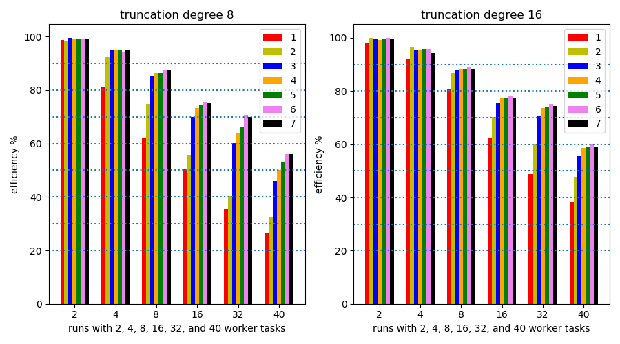
Figure 2: Efficiency plots for power series truncated to degrees 8 and 16, for 2, 4, 8, 16, 32, and 40 worker tasks, for seven precisions: double (d), 2-d, 3-d, 4-d, 5-d, 8-d, and 10-d, in the plots labeled respectively by bars 1, 2, 3, 4, 5, 6, and 7.

The plots in Figure 2 show efficiencies for degrees 8 and 16 of the truncated power series. The efficiencies decrease from close to 100% (a near perfect speedup for 2 threads) to below 60% when 40 worker threads are used. As efficiency equals speedup divided by the number of worker threads, the speedup corresponding to 60% efficiency for 40 worker threads equals $0.6\times 40=24$.

The plots in Figure 3 compare the efficiencies for degrees 16 and 32. For truncation degree 32, we observe that 60% efficiency is reached already at triple double precision. More extensive numerical experiments would increase the number of polynomials and the number of monomials per polynomial to investigate the notion of isoefficiency. In particular, by how much should the size of the problem increase to obtain the same efficiency as the number of threads increases?

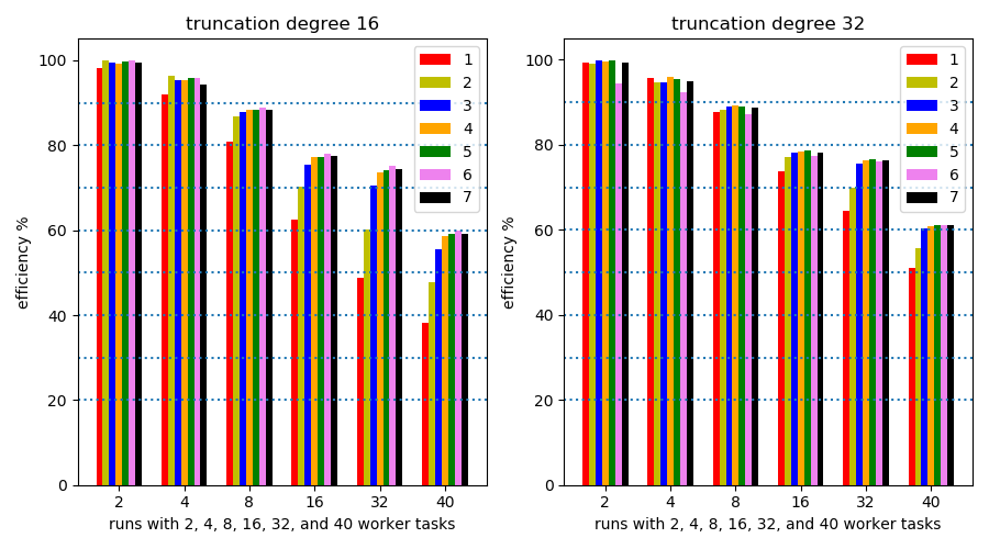
Figure 3: Efficiency plots for power series truncated to degrees 16 and 32, for 2, 4, 8, 16, 32, and 40 worker tasks, for seven precisions: double (d), 2-d, 3-d, 4-d, 5-d, 8-d, and 10-d, in the plots labeled respectively by bars 1, 2, 3, 4, 5, 6, and 7.

The computational results of this section (the 60% efficiency or the 24 speedup) justify the multiplication factor of 20 used in the last paragraph of section 6.

8. Conclusions

This paper presents a use case of multiple double precision in the application of Newton’s method to develop power series expansions for solution curves of polynomial systems. The experiments described in this paper are performed by recent additions to the free and open source software PHCpack, available via github.

PHCpack contains an Ada version of the code in QDlib [6], for double double and quad double precision, and of code generated by the software CAMPARY [7], for triple, penta, octo, and deca double precision. The cost overhead factors of multiple double precision are multiplied with the cost overhead factors of truncated power series arithmetic. This cost overhead justifies the application of multitasking to write parallel software. Using all kernel threads on a 44-core computer, numerical experiments that took about 5 hours are estimated to take more than four days without multitasking.

The efficiency of the current implementation is limited by the medium grained parallelism and may not scale well on shared memory computers with over one hundred cores. In refining the granularity of the current implementation, the Ada 202X parallel features look promising.

Acknowledgments. The author thanks Clyde Roby, Tucker Taft, and Richard Wai, the organization committee of the HILT 2020 Workshop on Safe Languages and Technologies for Structured and Efficient Parallel and Distributed/Cloud Computing. Earlier versions of the software were presented in the Ada devroom at FOSDEM 2020. The author is grateful to Dirk Craeynest and Jean-Pierre Rosen for the organization of the FOSDEM 2020 Ada devroom.

References

- [1] G. A. Baker and P. Graves-Morris. Padé Approximants, volume 59 of Encyclopedia of Mathematics and its Applications. Second edition, Cambridge University Press, 1996.
- [2] A. Burns and A. Wellings. Concurrent and Real-Time Programming in Ada. Cambridge University Press, 2007.
- [3] N. Bliss and J. Verschelde. The method of Gauss-Newton to compute power series solutions of polynomial homotopies. Linear Algebra and Its Applications 542:569–588, 2018.
- [4] G. H. Golub and C. F. Van Loan. Matrix Computations. The Johns Hopkins University Press, 1983.
- [5] A. Griewank and A. Walther. Evaluating Derivatives: Principles and Techniques of Algorithmic Differentiation. SIAM, 2008.
- [6] Y. Hida, X. S. Li, and D. H. Bailey. Algorithms for quad-double precision floating point arithmetic. In the Proceedings of the 15th IEEE Symposium on Computer Arithmetic (Arith-15 2001), pages 155–162. IEEE Computer Society, 2001.
- [7] M. Joldes, J.-M. Muller, V. Popescu, W. Tucker. CAMPARY: Cuda Multiple Precision Arithmetic Library and Applications. In Mathematical Software – ICMS 2016, the 5th International Conference on Mathematical Software, pages 232–240, Springer-Verlag, 2016.
- [8] J. W. McCormick, F. Singhoff, and J. Hugues. Building Parallel, Embedded, and Real-Time Applications with Ada. Cambridge University Press, 2011.
- [9] A. Morgan. Solving Polynomial Systems using Continuation for Engineering and Scientific Problems, volume 57 of Classics in Applied Mathematics. SIAM, 2009.
- [10] J.-M. Muller, N. Brunie, F. de Dinechin, C.-P. Jeannerod, M. Joldes, V. Lefevre, G. Melquiond, N. Revol, S. Torres. Handbook of Floating-Point Arithmetic. Second Edition, Springer-Verlag, 2018.
- [11] S. M. Rump. Verification methods: Rigorous results using floating-point arithmetic. Acta Numerica 19:287–449, 2010.
- [12] S. Telen, M. Van Barel, and J. Verschelde. A robust numerical path tracking algorithm for polynomial homotopy continuation. SIAM Journal on Scientific Computing 42(6):A3610–A3637, 2020.
- [13] S. Telen, M. Van Barel, and J. Verschelde. Robust numerical tracking of one path of a polynomial homotopy on parallel shared memory computers. In the Proceedings of the 22nd International Workshop on Computer Algebra in Scientific Computing (CASC 2020), volume 12291 of Lecture Notes in Computer Science, pages 563–582. Springer-Verlag, 2020.
- [14] J. Verschelde. Algorithm 795: PHCpack: A general-purpose solver for polynomial systems by homotopy continuation. ACM Transactions on Mathematical Software 25(2):251–276, 1999. Runs online at www.phcpack.org.
- [15] R. J. Walker. Algebraic Curves. Princeton University Press, 1950.