Colorful points in the $XY$ regime of $XXZ$ quantum magnets

In the $XY$ regime of the $XXZ$ Heisenberg model phase diagram, we demonstrate that the origin of magnetically ordered phases is influenced by the presence of solvable points with exact quantum coloring ground states featuring a quantum-classical correspondence. Using exact diagonalization and density matrix renormalization group calculations, for both the square and the triangular lattice magnets, we show that the ordered physics of the solvable points in the extreme $XY$ regime, at $\frac{J_{z}}{J_{\perp}}=-1$ and $\frac{J_{z}}{J_{\perp}}=-\frac{1}{2}$ respectively with $J_{\perp}>0$, adiabatically extends to the more isotropic regime $\frac{J_{z}}{J_{\perp}}\sim 1$. We highlight the projective structure of the coloring ground states to compute the correlators in fixed magnetization sectors which enables an understanding of the features in the static spin structure factors and correlation ratios. These findings are contrasted with an anisotropic generalization of the celebrated one-dimensional Majumdar-Ghosh model, which is also found to be (ground state) solvable. For this model, both exact dimer and three-coloring ground states exist at $\frac{J_{z}}{J_{\perp}}=-\frac{1}{2}$ but only the two dimer ground states survive for any $\frac{J_{z}}{J_{\perp}}>-\frac{1}{2}$.

I Introduction

The question of magnetic long-range ordering (LRO), or lack thereof, in quantum antiferromagnetic insulators in low dimensions has been of prime interest in the field of quantum magnetism. One of the hallmark results is the absence of true LRO for the quantum Heisenberg spin chain owing to strong quantum mechanical fluctuations in one dimension and the associated fractional spinon excitations. Giamarchi (2004) LRO does exist in two dimensions, but only at zero temperature, for the square lattice Heisenberg model, as well as other (unfrustrated) bipartite lattices. Chakravarty et al. (1989) In three dimensions, LRO exists at finite temperatures as well. Compounding this issue is the ingredient of frustration; it was initially suggested as a possible mechanism to suppress LRO in the triangular lattice Heisenberg antiferromagnet. Theoretical Huse and Elser (1988); Jolicoeur and Le Guillou (1989); Singh and Huse (1992); Bernu et al. (1992); Capriotti et al. (1999) and experimental studies Kadowaki et al. (1995); Ishii et al. (2011); Shirata et al. (2012) have revealed that LRO indeed survives in the triangular lattice geometry, however, other frustrated geometries and interactions have continued to be the subject of intense study.

Given the complexity of such problems, exactly solvable Hamiltonians form important cornerstones in our understanding of quantum magnetism and, more generally, quantum matter in its vast variety. Bethe’s solution of the one-dimensional ($1d$) Heisenberg chainBethe (1931) has led to an entire field of activity Guan et al. (2013); Karabach et al. (1997); Karbach et al. (1998); Levkovich-Maslyuk (2016) with Bethe ansatz methods applied to a host of $1d$ models including the spin-$\frac{1}{2}$ $XXZ$ model. Additionally, the ground state solvable one-dimensional Majumdar-Ghosh model Majumdar and Ghosh (1969), a precursor to the $S=1$ AKLT chain Affleck et al. (1987), has led to many insights into the valence bond physics of $1d$ frustrated systems. In higher dimensions, however, there are fewer solvable examples for both unfrustrated and frustrated quantum magnets, notably the Shastry-Sutherland model Shastry and Sutherland (1981) and Kitaev honeycomb model.Kitaev (2006) In this spirit, this work will show the influence of exactly solvable points in the $XXZ$ parameter space,

$$H_{XXZ}=J_{\perp}\sum_{\langle i,j\rangle}\left(S^{x}_{i}S^{x}_{j}+S^{y}_{i}S^{y}_{j}\right)+J_{z}\sum_{\langle i,j\rangle}S^{z}_{i}S^{z}_{j}$$ (1)

on magnetic LRO in two dimensional quantum antiferromagnets (QAFM). We will set $J_{\perp}=1$ throughout this paper.

The motivation for our present work stems from a recent finding of a higher-dimensional example of ground state solvable frustrated quantum magnets described by $H_{3c}\equiv H_{XXZ}[J_{z}=-1/2]$ Changlani et al. (2018) (previously referred to as “$XXZ0$”) on any lattice composed of triangular motifs that allow for a consistent “three-coloring" of the lattice sites where no two sites connected by a bond share the same color. Even though this work was situated in the context of the Kagome antiferromagnet, the general principle applies to a host of lattices including the triangular lattice. At this solvable $3c$ point, there is a one-to-one correspondence between the classical and quantum ground states. Adding realistic perturbations away from such a point in parameter space thus potentially offers a new way of understanding the phases that are stabilized by quantum fluctuations.

The coloring states remain exact ground states when projected to a specific magnetization sector due to $U(1)$ symmetry of the $XXZ$ model. This general projection structure of the exact ground state is an important feature of the solvable point, e.g. it was utilized Changlani et al. (2019) to explain the magnon crystal associated with the $\frac{m}{m_{s}}=\frac{7}{9}$ high-magnetization plateau state on the Kagome lattice Richter et al. (2004); Okuma et al. (2019); Schnack et al. (2020) where $m$ is the magnetization, and $m_{s}$ is its saturation value. This was achieved by an exact mapping of three-colorings to localized magnons using the projection structure (also see the recent Ref. Derzhko et al., 2020 for analogous mappings on the sawtooth lattice). The unprojected exact solution in the context of the triangular lattice has previously been noted by Ref. Momoi and Suzuki, 1992.

Here we address two cases with magnetic LRO - the frustrated triangular and unfrustrated square lattice which admit coloring ground states as shown in Fig. 1. For the unfrustrated case, the exact ground state corresponds to a two-coloring which is applicable for any bipartite lattice in any dimension and occurs for $J_{z}=-1$. Because of the projection structure of these states, we work in fixed magnetization sectors of choice. For the square lattice case, we focus on the zero magnetization sector and for the triangular case on the $m=0$ and $\frac{m}{m_{s}}=\frac{1}{3}$ sectors, the latter being a known plateau state at the Heisenberg point. Chubukov and Golosov (1991); Pal et al. (2020) For these projected coloring states, we establish the presence of magnetic LRO by calculating two-point correlators. Since these points in parameter space do not have the full $SU(2)$ but only $U(1)$ symmetry, the corresponding ground state in the zero magnetization sectors are AFM ordered in the $XY$ plane.

Figure 1: Illustration of the unique two-coloring on the square lattice, and one of the two three-colorings on the triangular lattice. The colorings directly correspond to magnetically ordered states.

We next investigate, using exact diagonalization (ED) and density matrix renormalization group (DMRG) White (1992); Fishman et al. (2020) calculations, how these coloring ground states are connected to the more isotropic regime $J_{z}\sim 1$. Using various measures, we provide evidence for the emergence of magnetic LRO in the square and triangular Heisenberg magnets from the solvable points. Interestingly, both the three-coloring and two-coloring solvable points sit at the quantum critical point between the $XY$ Néel LRO and ferromagnetic ground state. Thus, the exact ground states contain the seeds for both AFM and FM ordering. This basic structure of the $XXZ$ phase diagram for magnetically LRO magnets is the central result of this paper.

However, the presence of an exactly solvable point with quantum coloring ground states in the extreme anisotropic limit does not necessarily guarantee the existence of LRO away from it. We demonstrate this in the context of the anisotropic generalization of the celebrated Majumdar-Ghosh model where both coloring and dimer ground states are exact solutions at $J_{z}=-1/2$. The model is characterized by competing coloring and dimerized (valence bond) ground states; perturbing towards the isotropic point favors the dimer solutions rather than the coloring solutions.

The paper is organized as follows. In Sec. II, we discuss the case of the $m=0$ sector of the square lattice AFM in the context of the $J_{z}=-1$ point. In Secs. III.1 and III.2, we present our findings for the $m=0$ and $\frac{m}{m_{s}}=\frac{1}{3}$ sectors of the triangular AFM. As mentioned above, we contrast these findings with that for an anisotropic generalization of the Majumdar-Ghosh model in Sec. IV. In the appendices Apps. A-G, we provide derivations for correlations and structure factors induced by projection, applicable on any lattice and some additional useful information.

II The square lattice antiferromagnet

We consider the case of the Hamiltonian $H_{2c}\equiv H_{XXZ}[J_{z}=-1]$, where an exact ground state solution is guaranteed on any bipartite lattice in any dimension. We focus on the $2d$ square lattice where the existence of Néel LRO at the Heisenberg point $J_{z}=1$ is well establishedRichter et al. (2004), in comparison to the $1d$ chain which has only quasi-LRO with polynomially decaying spin-spin correlations. The ground state of $H_{2c}$ corresponds to a unique two-coloring of the bipartite lattice.

Let the two colors, denoted by red ($|r\rangle$) and blue ($|b\rangle$) labels, represent the $S^{x}$ eigenstates on a single site,

$$|r\rangle\equiv\frac{1}{\sqrt{2}}(|\uparrow\rangle+|\downarrow\rangle)\leavevmode\nobreak\ \leavevmode\nobreak\ \leavevmode\nobreak\ \leavevmode\nobreak\ \leavevmode\nobreak\ \leavevmode\nobreak\ \leavevmode\nobreak\ \leavevmode\nobreak\ \leavevmode\nobreak\ \leavevmode\nobreak\ |b\rangle\equiv\frac{1}{\sqrt{2}}(|\uparrow\rangle-|\downarrow\rangle).$$ (2)

The (unprojected) ground state at $H[J_{z}=-1]$ is

$$|C\rangle\equiv\left(\prod_{i\in A}\otimes_{i}|r\rangle_{i}\prod_{j\in B}\otimes_{j}|b\rangle_{j}\right)$$ (3)

where $A,B$ are the two sublattices of any bipartite lattice, for example, in 1D: chain, ladders; 2D: square, honeycomb; 3D: cube, hyper-honeycomb etc.

To show the ground state property of Eq. 3, we write $H_{2c}$ as a sum of bond Hamiltonians $H_{ij}\equiv S_{i}^{x}S_{j}^{x}+S_{i}^{y}S_{j}^{y}-S_{i}^{z}S_{j}^{z}$. On a given bond, the eigensystem of $H_{ij}[J_{z}=-1]$ consists of the polarized states $|\uparrow\uparrow\rangle$, $|\downarrow\downarrow\rangle$, and the bond singlet $|0;0\rangle\equiv(|\uparrow\downarrow\rangle-|\downarrow\uparrow\rangle)/\sqrt{2}$ as ground states with energy $-1/4$, while the state $|1;0\rangle\equiv(|\uparrow\downarrow\rangle+|\downarrow\uparrow\rangle)/\sqrt{2}$ is an excited state with energy $+3/4$. Then, $H_{ij}=\sum_{k=1}^{4}E_{k}|\psi_{k}\rangle\langle\psi_{k}|$ where $E_{k}$ are the four eigenenergies of the bond, and $|\psi_{k}\rangle$ are the corresponding eigenvectors. Using the identity $1=\sum_{k=1}^{4}|\psi_{k}\rangle\langle\psi_{k}|$, $H_{2c}=\sum_{\langle ij\rangle}H_{ij}$ is recast purely in terms of the bond projectors $P_{ij}\equiv|1;0\rangle\langle 1;0|$,

$$H_{2c} = \sum_{\langle ij\rangle}P_{ij}-\frac{1}{4}N_{\text{bonds}}$$ (4)

Since the coefficient in front of the projectors is positive, any wavefunction that simultaneously zeros out the projector on each bond is a ground state. Zeroing out a projector requires that only components orthogonal to $|1;0\rangle$ enter the many-body wavefunction. This is indeed achieved by $|C\rangle$. (Expanding out the product state for one $|r\rangle$ and one $|b\rangle$ gives $|\uparrow\uparrow\rangle-|\downarrow\downarrow\rangle-\sqrt{2}|0;0\rangle$, with each individual term being orthogonal to $|1;0\rangle$.)

One can see, at the level of a single bond, that there is inherent competition between FM ($|\uparrow\uparrow\rangle$,$|\downarrow\downarrow\rangle$) and AFM ($|0;0\rangle$) correlations, and the two states become exactly degenerate at $J_{z}=-1$. This, in turn, results in $J_{z}=-1$ being a critical point in the $XXZ$ phase diagram. Since total $S^{z}$ is conserved, the projected coloring state

$$|C_{S^{z}}\rangle\equiv P_{S^{z}}|C\rangle$$ (5)

is also the exact ground state in every $S^{z}$ sector, where $P_{S^{z}}$ is the projection to a given total $S^{z}$ sector. pro This construction gives a unique ground state in each total $S^{z}$ sector. For a lattice with $N$ sites, there are thus $(N+1)$ degenerate ground states which is readily verifiable in Exact diagonalization (ED) for accessible systems, as well as their ground state energy value (Table 1 in App. G).

Figure 2: For the square lattice $XXZ$ Hamiltonian in the $m=0$ sector, the left panel shows the ground state energy per bond ($E_{0}$) vs. $J_{z}$. The inset of the left panel shows the evolution of the structure factors ($\frac{S_{zz}(\mathbf{q}_{0})}{N}$ and $\frac{S_{xy}(\mathbf{q}_{0})}{N}$ such that they are intensive), calculated at the ordering vector $\mathbf{q}_{0}=(\pi,\pi)$. The right panel shows the correlation ratio, as defined in the text (Eq. 10), vs. $J_{z}$ at the ordering wave-vector $\mathbf{q}_{0}=(\pi,\pi)$ for the representative case of $\Delta\mathbf{q}=(\frac{2\pi}{L_{x}},0)$.

We note that the choice of the two colors in Eq. 2 has a (global) gauge freedom. The present choice is along the $X$ direction in $XY$ plane of the Bloch sphere. They can be chosen to be in any direction in the $XY$ plane owing to the $U(1)$ symmetry of $H[J_{z}]$. This is also seen at a classical level through a Luttinger-Tisza analysis of $H_{XXZ}$ which leads to a classical phase transition at $J_{z}=-1$, with a FM solution along the $Z$ axis for $J_{z}<-1$, and an AFM solution in the $XY$ plane for $J_{z}>-1$. This freedom of choice in direction in the $XY$ plane is the classical counterpart of the global gauge freedom seen in the quantum mechanical case. A similar classical-quantum correspondence works for $H_{3c}$.Changlani et al. (2019) In the classical case, the $XY$-plane AFM solution holds true only up to $J_{z}<1$, after which the AFM solution lies along the $Z$ axis. At $J_{z}=1$, the AFM solution can lie in any direction. In the quantum case, this translates to full $SU(2)$ symmetry at the Heisenberg point. We can thus anticipate that the $U(1)$ symmetric $XY$ Néel state as in Eq. 3 evolves in an adiabatic fashion to a $SU(2)$ symmetric Néel state, since both are essentially Néel-ordered states in the same total $S^{z}$ sector.

The above can also be understood as a consequence of a “superspin" with length $\frac{N}{2}$ with a degeneracy of $2\left(\frac{N}{2}\right)+1$, even though $H_{2c}$ is not $SU(2)$ symmetric and is short-ranged. A more familiar and direct example of such a superspin is rather the long-range all-to-all coupled $SU(2)$-symmetric Hamiltonian Lieb and Mattis (1962) $J\sum_{i\in A,j\in B}\left(S^{x}_{i}S^{x}_{j}+S^{y}_{i}S^{y}_{j}+S^{z}_{i}S^{z}_{j}\right)=J(\mathbf{S}_{A}\cdot\mathbf{S}_{B})$ where $\mathbf{S}_{A}$/$\mathbf{S}_{B}$ are superspins with length $\frac{N}{2}$. To see how this arises in $H_{2c}$, it is useful to compare its solution with that of the ferromagnetic Hamiltonian $H_{\text{FM}}=-H_{XXZ}[J_{\perp}=J_{z}]$ through a projector point of view. Recasting this ferromagnetic Hamiltonian as a sum of projectors, $H_{\text{FM}}=\sum_{\langle i,j\rangle}Q_{ij}$ after a trivial shift of $0.25$ per bond, where $Q_{ij}$’s are non-commuting semi-definite projectors to the singlet state $|0;0\rangle$ on bonds $\langle i,j\rangle$ respectively. The familiar eigensystem here is $|\uparrow\uparrow\rangle$, $|\downarrow\downarrow\rangle$ and $|1;0\rangle$ as ground states (with energy $-1/4$), and $|0;0\rangle$ as an excited state (with energy $+3/4$). The unprojected ground state is now achieved by $\prod_{i\in\{A,B\}}\otimes_{i}|r\rangle_{i}$, and projection to desired total $S^{z}$ sectors may again be done as before. Since total $\mathbf{S}^{2}$ is also conserved for $H_{\text{FM}}$, this projection gives rise to the usual multiplet structure expected for $SU(2)$ symmetry, i.e. the $2\left(\frac{N}{2}\right)+1=N+1$ degeneracy due to a superspin structure. Also, since we project out the singlet on each bond, we only get FM correlations here as expected. In contrast, for $H_{2c}$ there is no $SU(2)$ symmetry, and therefore the ground state in any total $S^{z}$ sector is a superposition of various total $\mathbf{S}^{2}$ sectors. Nonetheless, we see that the superspin structure of the ground state of $H_{\text{FM}}$ gets exactly mirrored in the ground state of $H_{\text{2c}}$ because of the close relation of the two ground states, $|C\rangle$ and $\prod_{i\in\{A,B\}}\otimes_{i}|r\rangle_{i}$. A phase change of $(-1)^{\#\downarrow_{B}}$ where $\#\downarrow_{B}$ are the number of down-spins on the B sublattice to the wavefunction coefficients (in the $S^{z}$ basis) maps uniquely $|C\rangle$ to $\prod_{i\in\{A,B\}}\otimes_{i}|r\rangle_{i}$ and vice versa, and this mapping carries over under projection $P_{S^{z}}$ as well.

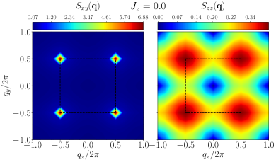
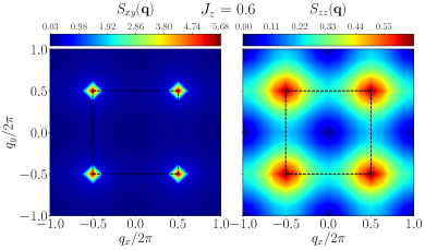
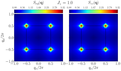
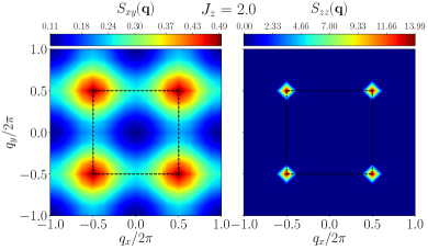
Figure 3: The panels show $S_{xy}(\mathbf{q})$ and $S_{zz}(\mathbf{q})$ for the square lattice, in the first Brillouin zone (highlighted by the dashed black lines) for various representative $J_{z}$ in the $m=0$ magnetization sector for the $N=8\times 8$ cylinder.

We now calculate the spin correlations in the state $|C_{S^{z}=0}\rangle$. Following Ref. Changlani et al., 2018’s supplementary, we have

$$\langle C_{S^{z}}|C_{S^{z}}\rangle\propto\frac{1}{N+1}\sum_{p}\prod_{j}\sum_{s_{j}}e^{ips_{j}}\langle c_{j}|s_{j}\rangle\langle s_{j}|c_{j}\rangle e^{-ipS^{*}_{z}}$$ (6)

up to an overall normalization, where $p$ runs from $0$ to $\frac{2\pi N}{N+1}$ in steps of $\frac{2\pi}{N+1}$, and $S^{*}_{z}$ is desired total $S^{z}$ sector. We work with even $N$ to ensure that $S^{*}_{z}=0$. $|c_{j}\rangle$ refers to the coloring of the site $j$ in $|C\rangle$, i.e. $|c_{j}\rangle=|r\rangle$ or $|b\rangle$ for $A$/$B$ sublattices respectively, and $|s_{j}\rangle$ are Ising states $|\pm\frac{1}{2}\rangle$. Taking into account the number of states in the $S^{*}_{z}=0$ sector compared to the full Hilbert space, we are guaranteed that $\langle C_{S^{z}=0}|C_{S^{z}=0}\rangle=\frac{1}{N+1}\frac{2^{N}}{{}^{N}C_{N/2}}\sum_{p}\left(\cos\frac{p}{2}\right)^{N}=1$ as expected. ${}^{N}C_{M}$ stands for the “$N$ choose $M$" combinatorial function everywhere in this paper, i.e. ${}^{N}C_{M}=N!/(M!(N-M)!)$. For the two-point correlators, we perform similar calculations and arrive at

$$\langle C_{S^{z}=0}|S^{z}_{m}S^{z}_{n}|C_{S^{z}=0}\rangle = -\frac{1}{4}\frac{1}{N-1}$$ (7)

$$\langle C_{S^{z}=0}|S^{x}_{m}S^{x}_{n}|C_{S^{z}=0}\rangle = \langle C_{S^{z}=0}|S^{y}_{m}S^{y}_{n}|C_{S^{z}=0}\rangle$$ (8)

$$= \frac{\epsilon_{mn}}{8}\frac{N}{N-1}$$

where $\epsilon_{mn}=-1$ for a pair of sites $\{m,n\}$ with different colors, and $\epsilon_{mn}=1$ for $\{m,n\}$ with the same color. These exact expressions are readily verifiable by performing ED on small systems (see Table 1). Details of the derivations are given in App. A. We see from the above that projection to $S^{z}=0$ sector introduces only sub-dominant corrections of $O(1/N)$ in the LRO correlations of $|C_{S^{z}=0}\rangle$ when compared to the unprojected state $|C\rangle$ which is another generic feature of the quantum-classical correspondence in all the examples considered in this paper, and are to be expected in other ordered cases as well.

We now show that the unprojected state $|C\rangle$ is a gapless ground state in the thermodynamic limit. Consider the following (unprojected) state $|C^{\prime}\rangle=\left(\prod_{i\in A}\otimes_{i}e^{iS_{i}^{z}\delta_{i}}|r\rangle_{i}\prod_{j\in B}\otimes_{j}e^{iS_{j}^{z}\delta_{j}}|b\rangle_{j}\right)$ built by modulating the two-colorings of $|C\rangle$ in the $XY$ plane of the Bloch sphere by a small angle $\delta_{i}$ that oscillates at a non-zero wavevector $\mathbf{q}\rightarrow 0$, e.g. $\delta_{i}=\delta\sin(\mathbf{q}\cdot\vec{r}_{i})$ with a small $\delta$. This variational state is like a Goldstone mode associated with $U(1)$-symmetry breaking, however it is not orthogonal to $|C\rangle$. Thus, for an excited state, we consider the following variational state $|\psi\rangle\propto|C^{\prime}\rangle-\langle C|C^{\prime}\rangle|C\rangle$. $|\psi\rangle$ is orthogonal to $|C\rangle$ by construction. The variational estimate for the excitation energy $\Delta E\equiv\langle\psi|H|\psi\rangle/\langle\psi|\psi\rangle-\langle C|H|C\rangle$ scales to zero as $N\rightarrow\infty$, provided the variational parameter $\delta$ is chosen to scale as $N^{\alpha}$ with $-1/2<\alpha<0$. The details are given in App. B. The foregoing discussions are thus highly suggestive of $|C_{S^{z}=0}\rangle$ (and $|C\rangle$) being adiabatically connected to the $SU(2)$ symmetric Néel ground state, which we numerically demonstrate next for the case of two dimensions and expect to hold for higher dimensions.

To analyze the magnetic structure and adiabaticity of the $XY$ LRO upto the $SU(2)$ symmetric Heisenberg point, we calculate the structure factors defined by

$$S_{zz}(\mathbf{q}) = \frac{1}{N}\sum_{m,n}e^{-i\mathbf{q}\cdot(\textbf{r}_{m}-\textbf{r}_{n})}\langle S^{z}_{m}S^{z}_{n}\rangle$$

$$S_{xy}(\mathbf{q}) = \frac{1}{N}\sum_{m,n}e^{-i\mathbf{q}\cdot(\textbf{r}_{m}-\textbf{r}_{n})}\frac{\langle S^{x}_{m}S^{x}_{n}\rangle+\langle S^{y}_{m}S^{y}_{n}\rangle}{2}$$ (9)

where we set $L_{x}$, $L_{y}$ as the number of unit cells along the primitive lattice directions such that the number of sites $N=L_{x}\times L_{y}$, and $\mathbf{r}_{m}$ is the Bravais lattice vector for site $m$, while $\mathbf{q}$ is a reciprocal lattice vector in the (first) Brillouin zone. We also calculate correlation ratios defined as

$$R_{\alpha}=1-\frac{S_{\alpha}(\mathbf{q}_{0}-\Delta\mathbf{q})}{S_{\alpha}(\mathbf{q}_{0})}\leavevmode\nobreak\ ,$$ (10)

where $\alpha\in(zz,xy)$, $\mathbf{q}_{0}$ is a chosen wave vector in the Brillouin zone, and $\mathbf{q}_{0}-\Delta\mathbf{q}$ represents one choice of the nearest wave vectors allowed on the discrete lattice. This quantity scales to $1$ if there is a Bragg peak at $\mathbf{q}_{0}$ implying ordering at that wavevector in the $\alpha$ channel, and scales to $0$ if there is no such ordering. This ratio is designed to approach unity independent of the strength of quantum fluctuations as long as there is spin LRO at the chosen wave vector.

For the square lattice, the two structure factors $S_{zz}(\mathbf{q_{0}})$ and $S_{xy}(\mathbf{q_{0}})$ at $\mathbf{q}_{0}=(\pi,\pi)$ are useful order parameters to measure the diagonal or Ising AFM ordering, and off-diagonal or $U(1)$/$XY$ AFM ordering respectively. In Fig. 2, we show the ground state energy per bond, and the above order parameters and corresponding correlation ratios at the AFM ordering wave vector $\mathbf{q}_{0}=(\pi,\pi)$ computed using ED and DMRG (with bond dimension $8000$) in the zero magnetization sector. From Fig. 2(a), we see a monotonic behavior in the ground state energy in the $XY$ regime extending up to $J_{z}=-1$ on one side and $J_{z}=1$ on the other side. This is the first piece of data that signals that a single phase encompasses the regime $J_{z}\in(-1,1)$ of the $XXZ$ phase diagram on the square lattice. At the end points of this regime, we observe kinks in the ground state energy curves.Bishop et al. (2017) At $J_{z}=-1$, this kink behavior is quite pronounced, and it corresponds to development of ferromagnetic order.

On the other hand, at $J_{z}=1$, the kink behavior is less pronounced. However, by looking at the structure factors in the inset of Fig. 2(a), we see that $S_{zz}(\mathbf{q}_{0})$ dominates over $S_{xy}(\mathbf{q}_{0})$ on the Ising side. This is consistent with the development of Ising AFM order Cuccoli et al. (2003), which is confirmed by the fact that $R_{zz}$ is essentially one on this side in Fig. 2(b). Germane to the solvable point $2c$ and as is also seen from Eq. 9, we observe that $R_{xy}$ tends to one strongly in the whole regime $J_{z}\in(-1,1)$. This second piece of data convincingly establishes that the $U(1)$ AFM LRO state at $J_{z}=-1$ is adiabatic all the way to the $SU(2)$-symmetric point. Our results show that the $XY$ regime of the square lattice unfrustrated magnet, and likely other unfrustrated magnets, has a ground state whose essential properties are captured by the correlations of the exact ground state $|C_{S^{z}=0}\rangle$. We finally note that the FM-AFM phase transition at $H_{2c}$ is a first-order level-crossing transition as can be seen in Fig. 2(a).

Our findings in Fig. 2 are further substantiated in Fig. 3 where we have plotted the full structure factor as a function of $\bf{q}$ for the $8(L_{x})\times 8(L_{y})$ cylinder. At $J_{z}=-2$ (top left), there is ferromagnetic order in the system. Imposing the constraint of $S_{z}=0$ in our DMRG calculations leads to a state with two domains arranged along the length of the cylinder, preserving the translational invariance along the $y$-direction due to periodic boundary conditions imposed in the $y$-direction. As a result of this modulation in the $x$-direction, the ordering wavevector in the $zz$ channel is not $(0,0)$. Instead, peaks occur at the smallest allowable nonzero $|q_{x}|=\frac{2\pi}{L_{x}}$ and $q_{y}=0$. The contributions to $S_{xx}(\mathbf{q})$ throughout the entire Brillouin zone are significantly smaller and arise purely near the domain wall due to transverse spin fluctuations (see App. F for real space plots of the spin-spin correlations for further discussion). Moving on to $J_{z}=-1$ (top right), DMRG correctly captures the exact two-coloring ground state; for this state the Fourier transform of the real space spin-spin correlators corresponding to the two-coloring wavefunction (Eq. 7 and Eq. 8) can be computed analytically (App. E). $S_{zz}(\mathbf{q})$ is precisely $1/4$ at all points in the first Brillouin zone except for $\mathbf{q}=(0,0),$ where its value is exactly zero. This is a direct consequence of the sum-rule $S_{zz}(0,0)=\frac{1}{N}\langle(\sum_{i=1}^{N}{S^{i}_{z}})^{2}\rangle=0$ where $N=L_{x}L_{y}$. $S_{xy}(\mathbf{q})$ has a Bragg peak at $\mathbf{q}_{0}=(\pi,\pi)$ and no peaks elsewhere as might be expected from the quantum-classical correspondence mentioned previously.

These features associated with perfect co-planar Néel order in $S_{xy}(\mathbf{q})$ are quantitatively modified on moving towards the Heisenberg point. For $S_{zz}(\mathbf{q})$, there is also a qualitative reorganization of spectral weight. The featureless $S_{zz}(\mathbf{q})$ at $J_{z}=-1$ now starts to develop a maximum at $\mathbf{q_{0}}$. For example, at $J_{z}=0.0$ (middle left) the dip at $(0,0)$ has broadened out significantly. As $J_{z}$ keeps increasing, the maxima at $\mathbf{q_{0}}$ also acquire appreciable weight as shown for $J_{z}=0.6$ (middle right). These features are further enhanced as one approaches the Heisenberg regime, and at exactly $J_{z}=1$ (bottom left) both correlators become identical due to $SU(2)$ symmetry. Beyond $J_{z}>1$ (bottom right), the dominant correlations are now present in the $zz$ channel seen clearly as a Bragg peak at $\mathbf{q}_{0}$ reflecting Ising LRO, while there are no peaks in the $XY$ channel but only a broad maximum at $\mathbf{q}_{0}$ in agreement with lack of $U(1)$ AFM LRO as surmised from $R_{xy}$ on the Ising side in Fig. 2.

III The triangular lattice antiferromagnet

III.1 Zero magnetization sector

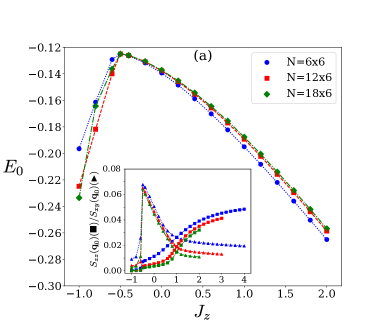
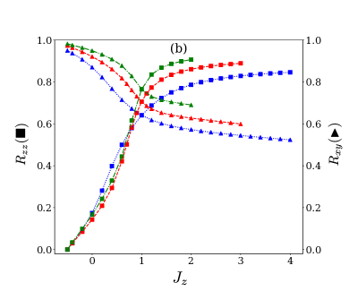
Figure 4: For the triangular lattice $XXZ$ Hamiltonian in the $m=0$ sector, the left panel shows the ground state energy per bond ($E_{0}$) vs. $J_{z}$ The inset of the left panel shows the evolution of the structure factors ($\frac{S_{zz}(\mathbf{q}_{0})}{N}$ and $\frac{S_{xy}(\mathbf{q}_{0})}{N}$), calculated at the ordering vector $\mathbf{q}_{0}=(4\pi/3,0)$. The right panel shows the correlation ratios ($R_{zz}$ and $R_{xy}$), as defined in the text (Eq. 10), vs. $J_{z}$ at the ordering wave-vector $\mathbf{q}_{0}$ for the representative case of $\Delta\mathbf{q}=(\frac{2\pi}{L_{x}},\frac{4\pi}{\sqrt{3}L_{y}}-\frac{2\pi}{\sqrt{3}L_{x}})$.

In this and the next section, we turn our attention to the triangular lattice AFM with its frustrated geometry. This geometry harbors a different solvable point $H_{3c}$ at $H[J_{z}=-1/2]$ as introduced in Sec. I such that the exact ground states are three-coloring states. On the triangular lattice, there are two distinct such ground states one which is sketched in Fig. 1. Analogous to the two-coloring case, these ground states also possess LRO in the $XY$ plane. Based on our knowledge of the $120^{\circ}$ ordered Heisenberg point Richter et al. (2004), we expect that LRO of the solvable point $H_{3c}$ extends to the $SU(2)$ symmetric point analogous to the situation on the square lattice.

In the zero magnetization sector, the two ground states may be written down as

$$|C^{(1)}_{Sz=0}\rangle \equiv P_{S^{z}=0}\left(\prod_{i\in A}\otimes_{i}|r\rangle_{i}\prod_{j\in B}\otimes_{j}|b\rangle_{j}\prod_{k\in C}\otimes_{k}|g\rangle_{k}\right)$$

$$|C^{(2)}_{S^{z}=0}\rangle \equiv P_{S^{z}=0}\left(\prod_{i\in A}\otimes_{i}|r\rangle_{i}\prod_{j\in B}\otimes_{j}|g\rangle_{j}\prod_{k\in C}\otimes_{k}|b\rangle_{k}\right)\;\;\;\;\;\;\;\;$$ (11)

where $A/B/C$ are the three sublattices, and $|r\rangle\equiv\frac{1}{\sqrt{2}}(|\uparrow\rangle+|\downarrow\rangle)$, $|b\rangle\equiv\frac{1}{\sqrt{2}}(|\uparrow\rangle+\omega|\downarrow\rangle)$ and $|g\rangle\equiv\frac{1}{\sqrt{2}}(|\uparrow\rangle+\omega^{2}|\downarrow\rangle)$. $\omega=e^{i2\pi/3}$ and $\omega^{2}=\omega^{*}$ are the cube roots of unity. $|r\rangle,|b\rangle,|g\rangle$ may be chosen to be any triad of $120^{\circ}$ states in the $XY$ plane of the Bloch sphere due to the presence of $U(1)$ symmetry, this choice being a global gauge choice.

Based on the existence of the $J_{z}=-\frac{1}{2}$ point coupled with linear spin-wave calculations, Ref. Momoi and Suzuki, 1992 argued the adiabaticity of the coloring ground states to the ground state at the $SU(2)$ point. In what follows, we will work in a fixed magnetization sector and numerically demonstrate this adiabaticty working with projected wavefunctions by calculating structure factors and correlation ratios.

For the $N$ site triangular lattice, the overlap between the two three-coloring states is given by

$$\langle C^{(k)}_{S^{z}=0}|C^{(l)}_{S^{z}=0}\rangle=\begin{cases}1,&\text{for $k=l$}.\\ \frac{{{}^{N/3}}C_{N/6}}{{{}^{N}}C_{N/2}},&\text{for $k\neq l$}.\end{cases}$$ (12)

where $k,l\in(1,2)$. It goes to zero for $k\neq l$ exponentially as $N\to\infty$ due to the macroscopic difference in the colors in the two wavefunctions. Perturbing away from the $3c$ point towards the Heisenberg point brings in matrix elements with magnitude that are exponentially small in $N$ between $|C^{(1)}\rangle$ and $|C^{(2)}\rangle$ at lowest-order resulting in an exponentially small splitting. As one goes further away from the $3c$ point, non-perturbative effects result in a finite splitting such that there is a unique ground state at the Heisenberg point. Alternatively, this can be understood by starting at the Heisenberg point which, being fully $SU(2)$-symmetric, harbors the low-energy quasi-degenerate Anderson tower of states whose energy spectrum is given by $\sim\frac{S(S+1)}{N}$. Lhu Appropriate linear combinations of these states are known to give symmetry broken states. Bernu et al. (1992) Thus, the effect of $XY$ anisotropy is to break this quasi-degeneracy of the Heisenberg point and lead to the (two) AFM ordered states. At and near the Heisenberg point, these states have significant quantum fluctuations White and Chernyshev (2007) which become effectively absent at the $3c$ point (Eq. 11).

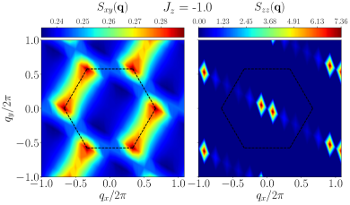
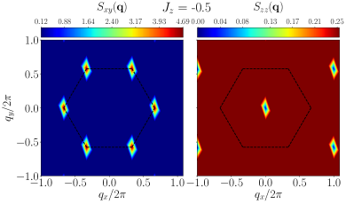
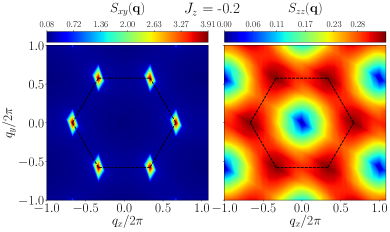
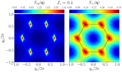
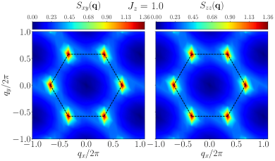
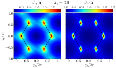
Figure 5: The panels show $S_{xy}(\mathbf{q})$ and $S_{zz}(\mathbf{q})$ for the triangular lattice in the first Brillouin zone (highlighted by the dashed black lines) for various representative $J_{z}$ in the $m=0$ magnetization sector for the $N=12\times 6$ cylinder.

A similar calculation (see App. C) for the correlators in either of the two ground states gives

$$\langle C^{(k)}_{S^{z}=0}|S^{z}_{m}S^{z}_{n}|C^{(k)}_{S^{z}=0}\rangle = -\frac{1}{4}\frac{1}{N-1}$$ (13)

$$\langle C^{(k)}_{S^{z}=0}|S^{x}_{m}S^{x}_{n}|C^{(k)}_{S^{z}=0}\rangle = \langle C^{(k)}_{S^{z}=0}|S^{y}_{m}S^{y}_{n}|C^{(k)}_{S^{z}=0}\rangle$$ (14)

$$= \frac{\epsilon_{mn}}{8}\frac{N}{N-1}$$

where $\epsilon_{mn}=-1/2$ for a pair of sites $\{m,n\}$ with different colors, and $\epsilon_{mn}=1$ for $\{m,n\}$ with the same color. For $N\rightarrow\infty$, $\langle S^{z}_{m}S^{z}_{n}\rangle\rightarrow 0$ and $\langle S^{x}_{m}S^{x}_{n}\rangle\propto\epsilon_{mn}$ reflect the three sublattice or $120^{\circ}$ order solely lying in the $XY$-plane.

The structure factors (Eq. 9) $S_{zz}(\mathbf{q_{0}})$ and $S_{xy}(\mathbf{q_{0}})$ at $\mathbf{q}_{0}=(\pm 4\pi/3,0)$ are useful order parameters for this case. They quantify the presence or absence of “diagonal" and “off-diagonal" LRO respectively in terms of the mapping between $S=\frac{1}{2}$ degrees of freedom and hardcore bosons ($S^{+}_{m}\to b^{\dagger}_{m}$, $S^{-}_{m}\to b_{m}$ and $S^{z}_{m}\to b^{\dagger}_{m}b_{m}-1/2$ on site $m$). If $S_{zz}(\mathbf{q})$ is finite as $N\to\infty$, the system has a broken sublattice $S^{z}$ symmetry which corresponds to the boson occupation density wave at wavevector $\mathbf{q}$, whereas a finite $S_{xy}(\mathbf{q})$ as $N\to\infty$ represent a broken $U(1)$ rotational symmetry which corresponds to superfluid ordering of the bosons. Sellmann et al. (2015)

In Fig. 4(a), we show the ground state energy per bond using both ED on toric and DMRG (with bond dimension $7000$) on cylindrical geometries. Its behavior is featureless as we scan from $H_{3c}$ to the Heisenberg point and beyond when compared to the corresponding data set for the square lattice (Fig. 2(a)). In the inset of Fig. 4(a), we show the magnitude of structure factors at the ordering vector $\mathbf{q}_{0}=(4\pi/3,0)$. In the range $-0.5<J_{z}<1$, $S_{xy}(\mathbf{q}_{0})$ dominates over $S_{zz}(\mathbf{q}_{0})$. Their finite size dependence suggests the absence of boson occupation ordering, and the presence of three-sublattice AFM LRO lying in the $XY$-plane tied to the $3c$ point (Eq. 14) corresponding to the superfluid state in the hardcore boson language. In contrast, $S_{zz}(\mathbf{q}_{0})$ dominates over $S_{xy}(\mathbf{q}_{0})$ for $J_{z}>1$. The finite size dependence of $S_{zz}(\mathbf{q}_{0})$ clearly shows the presence of boson occupation order in this regime. Moreover, the finite size dependence of $S_{xy}(\mathbf{q}_{0})$ suggests a coexistence of superfluid ordering in this regime, i.e. supersolid order, in agreement with earlier studies. Wang et al. (2009); Jiang et al. (2009); Heidarian and Paramekanti (2010)

However, inferring the thermodynamic behavior from the finite size dependence of order parameters can sometimes be inconclusive, especially if the extrapolated value is small as is the case for $S_{xy}(\mathbf{q}_{0})$ for $J_{z}>1$ (inset of Fig. 4(a)). In such situations, correlation ratios as defined in Eq. 10, have proved especially useful since they have been shown to be less susceptible to finite size effects.Pujari et al. (2016) Thus, we utilize them to probe the coexistence of density wave and superfluid LRO for $J_{z}>1$ which is shown in Fig. 4(b), choosing a representative $\Delta\mathbf{q}$ for computations. In the $XY$ regime, we see that $R_{xy}$ tends towards unity with increasing system size, while $R_{zz}$ decreases towards zero. This is consistent with the presence of $120^{\circ}$ AFM in the $XY$ plane or superfluid order. As we go beyond the Heisenberg point ($J_{z}>1$), we see that $R_{zz}$ now increases towards one providing evidence for boson density wave ordering. Furthermore, we see that $R_{xy}$ is quite appreciable and evidently consistent with a non-zero value that is increasing towards unity as we go towards the thermodynamic limit for the system sizes studied here. This provides strong evidence for the coexistence of superfluid and boson density ordering in the zero magnetization sector of the triangular AFM on the Ising side.

Given the unusual coexistence of diagonal and off-diagonal orders presented above unlike the square lattice case discussed in the previous section, we address how they are reflected in the spin structure factors. For the $12\times 6$ cylinder we plot $S_{zz}(\mathbf{q})$ and $S_{xy}(\mathbf{q})$ as a function of $J_{z}$ (Fig. 5). Our findings bear many qualitative similarities to the square lattice case on the $XY$ side. At $J_{z}=-1$ (top left), there is ferromagnetic order in the system with domains, and accordingly, the peaks in $S_{zz}(\mathbf{q})$ occur at the smallest allowable nonzero $|q_{x}|=\frac{2\pi}{L_{x}}$ and the corresponding $q_{y}$. Then, at $J_{z}=-1/2$ (top right), DMRG spontaneously picks one of the two three-colorings, and the features seen can be matched by exact computations (Eqs. 13,  14, App. E, also see App. F). $S_{zz}(\mathbf{q})$ is again precisely $1/4$ at all points in the first Brillouin zone except for $\mathbf{q}=(0,0),$ where its value is exactly zero. $S_{xy}(\mathbf{q})$ has Bragg peaks at $\mathbf{q}_{0}=(\frac{4\pi}{3},0)$ and symmetry related points in the Brillouin zone. For $J_{z}>-1/2$, the sequence of panels in Fig. 5 from $J_{z}=-0.2$ to $J_{z}=1.0$ confirm that the features associated with perfect coplanar $120^{\circ}$ order at $J_{z}=-1/2$ are only quantitatively modified on moving towards the Heisenberg point. Beyond $J_{z}>1$ (bottom right), the correlations are again dominated by the $zz$ channel with pronounced Bragg peaks seen at $\mathbf{q}_{0}$ signaling the diagonal LRO. However, the maxima in the $XY$ channel at $\mathbf{q}_{0}$ are also Bragg peaks as confirmed through the size dependence of correlation ratio $R_{xy}$ on the Ising side (Fig. 4) which is the expected signature of the co-existence of superfluid LRO in the structure factor, as opposed to the square lattice case where only a broad maximum was present at the ordering wavevector $(\pi,\pi)$.

Our ED and DMRG results are in agreement with the previous studies that have focused on $J_{z}>0$. Our study shows that the properties on the $XY$ side originate from the $3c$ point including the $120^{\circ}$ order at the Heisenberg point. Thus, for zero magnetization, we may say that the Heisenberg points on triangular and square lattices are “inheriting" the long-range AFM order of their respective solvable points $H_{3c}$ and $H_{2c}$. Moreover, on the Ising side past the Heisenberg point, the correlation ratio data provides compelling evidence for the coexistence of diagonal and off-diagonal LRO.

III.2 $\frac{m}{m_{s}}=\frac{1}{3}$ sector

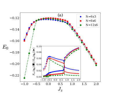
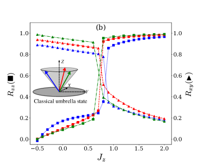
Figure 6: For the triangular lattice $XXZ$ Hamiltonian in the $\frac{m}{m_{s}}=\frac{1}{3}$ sector, the left panel shows the ground state energy per bond ($E_{0}$) vs. $J_{z}$. The inset of the left panel shows the evolution of the structure factors $\left(\frac{S_{zz}(\mathbf{q}_{0})}{N}\text{ and }\frac{S_{xy}(\mathbf{q}_{0})}{N}\right)$, calculated at the ordering vector $\mathbf{q}_{0}=(4\pi/3,0)$. The right panel shows the correlation ratios ($R_{zz}$ and $R_{xy}$) as defined in the text (Eq. 10) vs. $J_{z}$ plot at the ordering wave-vector $\mathbf{q}_{0}$ for the representative case of $\Delta\mathbf{q}=(\frac{2\pi}{L_{x}},\frac{4\pi}{\sqrt{3}L_{y}}-\frac{2\pi}{\sqrt{3}L_{x}})$. The inset of the right panel shows a schematic of classical spin configurations in the classical umbrella state that correspond to the corresponding three-colored sites (Fig. 1).

The ground state of the $\frac{m}{m_{s}}=\frac{1}{3}$ sector of the triangular Heisenberg AFM has been argued to be a magnetization plateau state. Chubukov and Golosov (1991); Alicea et al. (2009) In this state, each triangle has two spin-ups and one spin-down in a modulated pattern at the wave vector $\mathbf{q}_{0}=(4\pi/3,0)$ (the “UUD" state) which is equivalent to $\frac{1}{3}$ filling of hardcore bosons ordering at the same wave vector. A magnetization plateau state is an incompressible state with a gap to excitations that change magnetization. In contrast, coloring ground states are expected to be gapless with low energy Goldstone modes lying above it. At the classical level for $\frac{m}{m_{s}}=\frac{1}{3}$, the ground state in the $XY$ regime ($0<J_{z}<1$), is an “umbrella" state whose projection on to the $XY$ plane has $120^{\circ}$ correlations (see a schematic in the inset of Fig. 6). Yamamoto et al. (2014) This classical umbrella state in fact extends all the way to the $3c$ point. Since the $3c$ point exists for any magnetization sector, it is natural to ask how the quantum counterpart of the classical umbrella state that emerges from the $3c$ point eventually transitions to the magnetization plateau state.

Starting from Eq.(6) in this $\frac{m}{m_{s}}=\frac{1}{3}$ sector, i.e. setting $S^{*}_{z}=N/6$, gives

$$\langle C^{(k)}_{S^{z}=N/6}|C^{(l)}_{S^{z}=N/6}\rangle=\begin{cases}1,&\text{for $k=l$}.\\ \frac{{}^{N/3}C_{2N/9}}{{}^{N}C_{2N/3}},&\text{for $k\neq l$}.\end{cases}$$ (15)

and in the thermodynamic limit, the overlap between the two three-coloring ground state again goes to zero. Similarly, we have

$$\langle C^{(k)}_{S^{z}=N/6}|S^{z}_{m}S^{z}_{n}|C^{(k)}_{S^{z}=N/6}\rangle = -\frac{1}{4}\left[\frac{8}{9}\frac{N}{N-1}-1\right]$$ (16)

$$\langle C^{(k)}_{S^{z}=N/6}|S_{m}^{x}S_{n}^{x}|C^{(k)}_{S^{z}=N/6}\rangle = \langle C^{(k)}_{S^{z}=N/6}|S_{m}^{y}S_{n}^{y}|C^{(k)}_{S^{z}=N/6}\rangle$$ (17)

$$= \frac{\epsilon_{mn}}{9}\frac{N}{N-1}$$

where again $\epsilon_{mn}=-1/2$ for a pair of sites $\{m,n\}$ having different colors, while $\epsilon_{mn}=1$ for $\{m,n\}$ with same color. This again reflects $120^{\circ}$ sub-lattice LRO in the $XY$ plane in triangular lattice. As expected, $\langle S^{z}_{m}S^{z}_{n}\rangle$ is now finite as $N\to\infty$ in this nonzero magnetization sector with the thermodynamic value of this correlator in complete agreement with $\frac{m}{m_{s}}=\frac{1}{3}$. This along with $\langle S_{m}^{x}S_{n}^{x}\rangle\propto\epsilon_{mn}$ tells us that the state at the solvable point in this magnetization sector is the quantum counterpart of umbrella state illustrated in Fig. 6.

In Fig. 6(a), we show the ground state energy (per bond) for a wide range of $J_{z}$. It shows a sharp kink at $J_{z}^{c}\approx 0.75$ on the XY side, indicative of a first-order phase transition that occurs before the $SU(2)$-symmetric Heisenberg point. In the range $-0.5<J_{z}<J_{z}^{c}$, $S_{xy}(\mathbf{q}_{0})$ dominates over $S_{zz}(\mathbf{q}_{0})$ at $\mathbf{q}_{0}=(4\pi/3,0)$ in accordance with an umbrella state. Due to the net magnetization, $S_{zz}$ has a peak at the zero wavevector (not shown) for all $J_{z}$. Once $J_{z}>J^{c}_{z}$, $S_{zz}(\mathbf{q}_{0})$ becomes the dominant order parameter, while $S_{xy}(\mathbf{q}_{0})$ is suppressed in accordance with the UUD state.

We confirm the first-order nature of the transition using the correlation ratio as shown in Fig. 6(b): To the left of $J^{c}_{z}$, $R_{xy}$ tends to unity while $R_{zz}$ tends to zero. To the right of $J^{c}_{z}$, $R_{zz}$ tends towards unity, while $R_{xy}$ tends towards zero. In this magnetization sector, the finite size trends of the order parameter and the correlation ratio are clear-cut, and we clearly see the first-order behavior as sharp discontinuities in these quantities near $J^{c}_{z}$. Our results for $J_{z}>0$ are in agreement with previous work on the triangular phase diagram Yamamoto et al. (2014); Sellmann et al. (2015) and extend it to the solvable point. Through this work, we realize that the umbrella state in the phase diagram as actually being inherited from the $3c$ point, but quantum fluctuations eventually drive a phase transition to the UUD plateau state.

IV Colors and dimers in the anisotropic Majumdar-Ghosh chain

We now study a model which illuminates the competition between three-coloring states and other quantum ground states. Our inspiration stems from the Majumdar-Ghosh (MG) model, Majumdar and Ghosh (1969) one of the earliest known exactly solvable models of frustrated $1d$ quantum magnetism. The model has nearest neighbor $J_{1}$ and second neighbor $J_{2}$ isotropic Heisenberg interactions in the ratio $\frac{J_{2}}{J_{1}}=\frac{1}{2}$, which allows the Hamiltonian to be written as $H^{MG}=\frac{1}{2}\sum_{i=1}^{N}\Big{(}\vec{S}_{i-1}+\vec{S}_{i}+\vec{S}_{i+1}\Big{)}^{2}$ up to an innocuous constant for $N$ sites and periodic boundary conditions ($i+1$ and $i-1$ are taken modulo $N$). Each term in this sum corresponds to the square of the total spin of three consecutive sites schematically shown in Fig. 7.

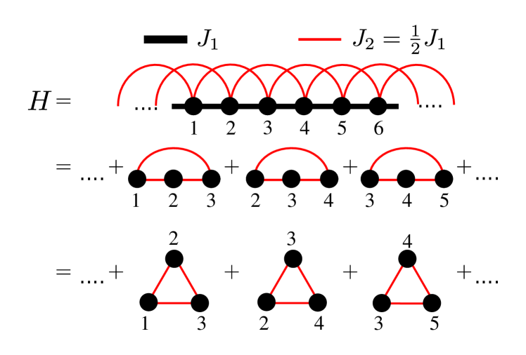
Figure 7: Decomposition of the Hamiltonian for the Majumdar-Ghosh chain (and its anisotropic generalization), which can be visualized as overlapping three site contiguous chunks. Each three site motif has the $XXZ$ Hamiltonian on a triangular motif which, at $J_{z}=-\frac{1}{2}$ can be three-colored and dimer covered consistently, without creating any conflicts.

For even $N$, all terms can be simultaneously minimized, a property of “frustration free" Hamiltonians, i.e. each three site motif can be brought in a total $S=\frac{1}{2}$ state in two different ways. These correspond to the two dimer coverings of the one dimensional chain and are referred to as the valence bond solid (VBS) states in the literature. Ref. Caspers et al., 1984 rigorously proved that these are the only two exact ground states of the MG chain.

We generalize the MG Hamiltonian to anisotropic interactions,

$$H^{MG}_{XXZ}= \>J_{1}\sum_{i=1}^{N}\left(S^{x}_{i}S^{x}_{i+1}+S^{y}_{i}S^{y}_{i+1}+J_{z}\>S^{z}_{i}S^{z}_{i+1}\right)+$$

$$J_{2}\sum_{i=1}^{N}\left(S^{x}_{i}S^{x}_{i+2}+S^{y}_{i}S^{y}_{i+2}+J_{z}\>S^{z}_{i}S^{z}_{i+2}\right)$$ (18)

with $\frac{J_{2}}{J_{1}}=\frac{1}{2}$ which we fix for the rest of this discussion, and $J_{z}$ is a dimensionless parameter in this section. For this ratio of $\frac{J_{2}}{J_{1}}=\frac{1}{2}$, the entire Hamiltonian still remains a sum of triangular pieces each of which has the $3c$ form for $J_{z}=-\frac{1}{2}$; this decomposition has been schematically depicted in Fig. 7. The ground state of this Hamiltonian is thus locally a three-coloring state on each triangular piece. As long as each of these three-site motifs can be three-colored consistently, without creating any “color conflicts" (no neighboring sites have the same color, and each contiguous three site motif has three distinct colors), the resulting wavefunction is an exact ground state of the anisotropic MG chain. For chain lengths that are multiples of three, this can be done in precisely two ways - $rbgrbg...$ and $rgbrgb...$, as is shown in Fig. 8. For chain lengths that are also even, i.e. multiples of six, we may project the two three-colorings to the $S_{z}=0$ sector and, as mentioned earlier, this projection still preserves the property that it is an eigenstate.

Additionally, the set of two dimer coverings are also exact ground states at the $3c$ point of the anisotropic MG chain. This is because on any three-site triangular motif, the two linearly independent three-colorings (schematically $|rgb\rangle$ and $|rbg\rangle$) may be linearly combined and then projected to $S_{z}=\pm\frac{1}{2}$ to make a dimer or valence bond and a free spin-$\frac{1}{2}$. Indeed, this is the situation at the familiar $J_{z}=1$ MG point as well. Requiring all three-site triangular motifs to have a dimer and a free spin-$\frac{1}{2}$ yields the two dimer covering states.

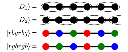
Figure 8: Dimer and three-color solutions on a six site motif. These patterns repeat for larger systems. For $J_{z}=-\frac{1}{2}$ all four states are exact ground states, for periodic chains that have sizes which are multiples of six. (For exactly six sites, the four solutions are not linearly independent). For $|D_{2}\rangle$, the sites on the boundary pair up into a dimer for periodic boundary conditions.

For a six-site chain, the proposed set of four solutions (two three-colorings and two dimer coverings) are not linearly independent. We establish this with an explicit enumeration of the amplitudes of three-coloring and dimer wavefunctions for all 20 Ising configurations in the $S_{z}=0$ sector (see Table 2 in App. G). We obtain the relation,

$$|D_{1}\rangle+|D_{2}\rangle=\frac{\sqrt{20}}{\omega^{2}-\omega}P_{S_{z}=0}(|rgbrgb\rangle-|rbgrbg\rangle)$$ (19)

where $|D_{1}\rangle$ and $|D_{2}\rangle$ are depicted in Fig. 8, and in our notation, $P_{S_{z}=0}|...\rangle$ corresponds to a coloring wavefunction that has been projected and normalized. In defining our sign convention for the dimer solutions, we have used that any local dimer of sites $i$ and $i+1$ (modulo N) is $\frac{1}{\sqrt{2}}\Big{(}|\uparrow\rangle_{i}\otimes|\downarrow\rangle_{i+1}-|\downarrow\rangle_{i}\otimes|\uparrow\rangle_{i+1}\Big{)}$. For chains that are higher multiples of six, there is no such linear dependence between the four states. On larger system sizes $N=12,18,24,30$, we find the number of solutions to be four or greater. We have empirically observed the precise number to be $(\frac{N}{6}+2)$ but do not have an explanation for the extra solutions.

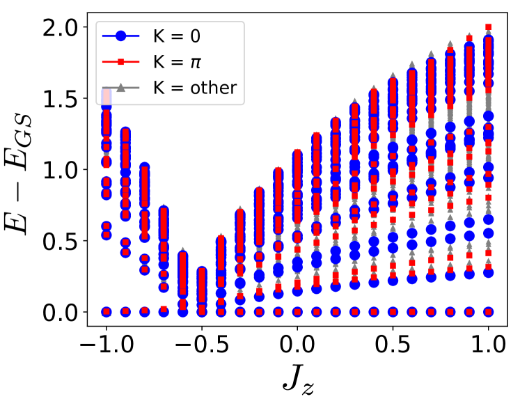
Figure 9: Energy spectrum of the 18 site periodic anisotropic Majumdar-Ghosh chain as a function of $J_{z}$ ($J_{\perp}=1$) in the $S_{z}=0$ sector. For a given $J_{z}$, only the lowest 30 energies in each momentum sector are plotted. The ground state energy is subtracted out at each value of $J_{z}$. There is a phase transition at $J_{z}=-\frac{1}{2}$. For $J_{z}>-\frac{1}{2}$ the ground state is exactly two fold degenerate (one state in $k=0$ and the other in $k=\pi$), which correspond to linear combinations of the two Majumdar-Ghosh dimer (valence bond) solutions. These ground states persist all the way to the Heisenberg point ($J_{z}=1$) and beyond (not shown), consistent with the analytic arguments.

We now address the case of $J_{z}\geq-\frac{1}{2}$. We rewrite the anisotropic MG Hamiltonian (up to a constant) as

$$H^{MG}_{XXZ} = H^{MG}_{3c}+\frac{(J_{z}+\frac{1}{2})}{2}\sum_{i=1}^{N}(S_{i-1}^{z}+S_{i}^{z}+S_{i+1}^{z})^{2}$$ (20)

$$\equiv H^{MG}_{3c}+H_{ZZ}$$

As the second term involves the square of the sum over only the $S^{z}$ components, therefore for $(J_{z}+\frac{1}{2})\geq 0$ this term is minimized for any state that satisfies $(S_{i-1}^{z}+S_{i}^{z}+S_{i+1}^{z})^{2}|\psi\rangle=(\frac{1}{2})^{2}|\psi\rangle$ for any three consecutive sites $\{i-1,i,i+1\}$. While $H^{MG}_{3c}$ and $H_{ZZ}$ do not commute, any wavefunction that simultaneously minimizes their individual contributions is guaranteed to be a ground state of the anisotropic MG model. This condition is indeed achieved by the dimer VBS states since, as discussed earlier, they respect the condition that any three-site triangular motif is composed of a dimer and a free spin-$\frac{1}{2}$. Thus, they are indeed the lowest energy eigenstates of $H^{MG}_{3c}$ and $H_{ZZ}$ simultaneously and therefore of $H^{MG}_{XXZ}$. This analytic result is confirmed with exact diagonalization, and demonstrated for the representative example of the 18 site periodic chain in Fig. 9. While the dimer solutions break translational invariance, appropriate linear combinations of them restore this symmetry, these linear combinations appear in exact diagonalization (with momentum symmetry). We observe two exactly degenerate states, one with momentum $k=0$ and the other $k=\pi$ that are selected from the degenerate manifold at $J_{z}=-\frac{1}{2}$, and stay degenerate for all $J_{z}>-\frac{1}{2}$, gapped out from the rest of the spectrum.

The three-coloring states (projected or unprojected) possess LRO, and in accordance with the Mermin-Wagner theorem are not allowed to be the ground state of a Hamiltonian with continuous symmetry in one dimension. However, at precisely the $J_{z}=-\frac{1}{2}$ point which is a critical point in parameter space, both the short range ordered solutions (dimer VBS) and the three-coloring states coexist. Chertkov and Clark (2018) This leads us to conclude that the presence of competing states at the solvable point can strongly influence the stability of the coloring ground state, and in this particular case, they immediately lose out to the VBS ground states for any $J_{z}>-\frac{1}{2}$.

V Conclusion

In this work, we have reported a ground state solvable point $H_{2c}$ in the $XXZ$ phase diagram of lattice translationally invariant bipartite quantum magnets in any magnetization sector. The associated $U(1)$ symmetric $XY$ Néel order in the zero magnetization sector is numerically demonstrated to be adiabatically connected to the $SU(2)$ symmetric Néel order at the Heisenberg point. This is unified with a similar thread in the tripartite triangular lattice with $120^{\circ}$ AFM order and associated solvable point $H_{3c}$ with finite number of three-colorings. For the case of the $\frac{m}{m_{s}}=\frac{1}{3}$ sector on the triangular lattice, we found that the umbrella state at $H_{3c}$ extends up to $J_{z}\sim 0.75$, after which the magnetization plateau UUD state is obtained. We also studied the anistropic generalization of the MG chain and found it to be ground state solvable. Both long-range ordered colorings and valence bond ordered states coexist at the $3c$ point, while the latter are the only ground states on moving towards the $SU(2)$-symmetric point and beyond. This offers an interesting contrast to the previous results that we presented on magnetic LRO.

It is also interesting to ask whether the existence of the $2c$ point offers a natural explanation for the numerically observed existence of LRO on diluted unfrustrated AFM at their percolation threshold. Yu et al. (2005); Wang and Sandvik (2006); Sandvik (2002); Kato et al. (2000); Changlani et al. (2013); Ghosh et al. (2015) This problem has seen several conflicting opinions, owing to the possible smallness of the order parameter (the staggered magnetization). Parts of the system become dimer covered with dominant VBS correlations, and hence magnetically inert, yet LRO tenuously survives on such fractal clusters. LRO at the $2c$ point on such bipartite clusters is obviously guaranteed (Eq. 8), and one would anticipate that it adiabatically persists to the Heisenberg point, but this remains to be firmly established.

In comparison to the ordered cases presented here, that involved finite number of colorings of the lattice, the highly-frustrated Kagome lattice harbors a macroscopic degeneracy due to an exponential number of three-colorings. Changlani et al. (2018) While it is not clear which state is stabilized as one moves towards the Heisenberg point, there is evidence of adiabaticity of the Heisenberg point to $H_{3c}$ from DMRG computations. He and Chen (2015); Läuchli and Moessner (2015); Changlani et al. (2019) Evidence for adiabaticity to the $XY$ point ($J_{z}=0$) was also observed previously in the context of chiral spin liquid on the Kagome lattice in the $m/m_{s}=2/3$ magnetization sector. Kumar et al. (2016) These findings suggest a unifying picture of the ground state behavior in $XXZ$ models. A natural question to ask then is what happens to the excited states and the associated dynamics of coloring states on tuning the anisotropy. (The question of non-equilibrium dynamics in the vicinity of the $3c$ point on the Kagome, as a function of anisotropy has been addressed recently Lee et al. (2020a, b)). Finally, for completeness, we note that our numerical evidence for adiabaticity from solvable points towards the isotropic regime strictly applies to finite size systems, and rigorously showing this in the thermodynamic limit at the level of a mathematical theorem is an open problem.

VI Acknowledgements

We acknowledge useful discussions with Johannes Richter, Nandini Trivedi, Subhro Bhattacharjee, Arnab Sen and Yasir Iqbal. SP acknowledges the support (17IRCCSG011) of IRCC, IIT Bombay and SERB, DST, India (SRG/2019/001419). HJC and PS acknowledge funds from Florida State University and the National High Magnetic Field Laboratory. The National High Magnetic Field Laboratory is supported by the National Science Foundation through NSF/DMR-1644779 and the state of Florida. We also thank the Research Computing Cluster (RCC) and the Planck cluster at Florida State University for computing resources.

Appendix A Two-point ground state correlators for $H_{2c}$

Here we calculate matrix elements for the unique two-coloring state $|C_{S^{z}=0}\rangle$ on any bipartite lattice with equal number of A and B sublattice sites. We start with the overlap $\langle C_{S^{z}=0}|C_{S^{z}=0}\rangle$ as in Eq. 6 to highlight the basic algebraic manipulations that will used throughout in these calculations. We recall that $|c_{j}\rangle$ can be either $|r\rangle\equiv\frac{1}{\sqrt{2}}(|\uparrow\rangle+|\downarrow\rangle)$ or $|b\rangle\equiv\frac{1}{\sqrt{2}}(|\uparrow\rangle-|\downarrow\rangle)$, and $|s_{j}\rangle$ are the Ising states $|\uparrow\rangle$ or $|\downarrow\rangle$ on site $j$. Terms of the form $\langle c_{j}|s_{j}\rangle$ follow from these definitions. Taking into account the overall normalization of $\frac{2^{N}}{{}^{N}C_{N/2}}$ in the $S^{*}_{z}=0$ sector as discussed in the main text, we have,

$$\langle C_{S^{z}=0}|C_{S^{z}=0}\rangle = \mathcal{N}\sum_{p}\prod_{j}\frac{1}{2}(e^{ip/2}+e^{-ip/2})\hskip 85.35826pt(\text{where}\leavevmode\nobreak\ \leavevmode\nobreak\ \mathcal{N}=\frac{1}{N+1}\frac{2^{N}}{{}^{N}C_{\frac{N}{2}}})$$ (21)

$$= \frac{\mathcal{N}}{2^{N}}\sum_{k=0}^{N}(e^{ik\theta}+e^{-ik\theta})^{N}\hskip 56.9055pt(\text{where}\leavevmode\nobreak\ \leavevmode\nobreak\ p=\frac{2\pi k}{N+1}=2k\theta\leavevmode\nobreak\ \leavevmode\nobreak\ \text{and}\leavevmode\nobreak\ \leavevmode\nobreak\ k\leavevmode\nobreak\ \text{ is integer})$$

$$= \frac{\mathcal{N}}{2^{N}}\sum_{k=0}^{N}\sum_{m=0}^{N}{{}^{N}C_{m}}(e^{ik\theta})^{m}(e^{-ik\theta})^{N-m}\hskip 56.9055pt(\text{using the binomial expansion})$$

$$= \frac{\mathcal{N}}{2^{N}}\sum_{m=0}^{N}{{}^{N}C_{m}}(N+1)\delta_{N/2-m,0}$$

$$= \mathcal{N}\frac{N+1}{2^{N}}{{}^{N}C_{\frac{N}{2}}}=1\leavevmode\nobreak\ .$$

as expected.

Analogous to Eq. 6, the general expression for diagonal correlation function in the zero magnetization sector is

$$\langle C_{S^{z}=0}|S^{z}_{m}S^{z}_{n}|C_{S^{z}=0}\rangle$$

$$= \mathcal{N}\sum_{p}\left[\left(\sum_{s_{m},s^{\prime}_{m},s_{n},s^{\prime}_{n}}e^{ips_{m}}\langle c_{m}|s_{m}\rangle\langle s_{m}|S^{z}_{m}|s^{\prime}_{m}\rangle\langle s^{\prime}_{m}|c_{m}\rangle\;e^{ips_{n}}\langle c_{n}|s_{n}\rangle\langle s_{n}|S^{z}_{n}|s^{\prime}_{n}\rangle\langle s^{\prime}_{n}|c_{n}\rangle\right)\left(\prod_{j\neq\{m,n\}}\sum_{s_{j}}e^{ips_{j}}\langle c_{j}|s_{j}\rangle\langle s_{j}|c_{j}\rangle\right)\right].$$

Perfoming the $s_{m},s^{\prime}_{m},s_{n},s^{\prime}_{n},s_{j}$ sums, we get

$$\langle C_{S^{z}=0}|S^{z}_{m}S^{z}_{n}|C_{S^{z}=0}\rangle = \mathcal{N}\sum_{p}\left[\frac{1}{4}(e^{ip/2}-e^{-ip/2})\frac{1}{4}(e^{ip/2}-e^{-ip/2})\prod_{j\neq\{m,n\}}\frac{1}{2}(e^{ip/2}+e^{-ip/2})\right]$$ (23)

$$= \mathcal{N}\sum_{p}\left[\frac{1}{4}\frac{(e^{ip/2}-e^{-ip/2})(e^{ip/2}-e^{-ip/2})}{(e^{ip/2}+e^{-ip/2})(e^{ip/2}+e^{-ip/2})}\prod_{j}\frac{1}{2}(e^{ip/2}+e^{-ip/2})\right]$$

$$= -\frac{\mathcal{N}}{2^{N+2}}\sum_{p}\left[(e^{ip/2}+e^{-ip/2})^{N-2}-(e^{ip/2}+e^{-ip/2})^{N}\right]$$

$$= -\frac{\mathcal{N}(N+1)}{2^{N+2}}[4\times^{N-2}C_{\frac{N}{2}-1}-^{N}C_{\frac{N}{2}}]$$

$$= -\frac{1}{4}\frac{1}{N-1}$$

where we use similar manipulations as in Eq. 21. Similarly, the general expression for off-diagonal correlation function in the zero magnetization sector is

$$\langle C_{S^{z}=0}|S^{\pm}_{m}S^{\mp}_{n}|C_{S^{z}=0}\rangle$$

$$= \mathcal{N}\sum_{p}\left[\left(\sum_{s_{m},s^{\prime}_{m},s_{n},s^{\prime}_{n}}e^{ips_{m}}\langle c_{m}|s_{m}\rangle\langle s_{m}|S^{\pm}_{m}|s^{\prime}_{m}\rangle\langle s^{\prime}_{m}|c_{m}\rangle\;e^{ips_{n}}\langle c_{n}|s_{n}\rangle\langle s_{n}|S^{\mp}_{n}|s^{\prime}_{n}\rangle\langle s^{\prime}_{n}|c_{n}\rangle\right)\left(\prod_{j\neq\{m,n\}}\sum_{s_{j}}e^{ips_{j}}\langle c_{j}|s_{j}\rangle\langle s_{j}|c_{j}\rangle\right)\right]\leavevmode\nobreak\ .$$

Again, perfoming the $s_{m},s^{\prime}_{m},s_{n},s^{\prime}_{n},s_{j}$ sums, we get

$$\langle C_{S^{z}=0}|S^{\pm}_{m}S^{\mp}_{n}|C_{S^{z}=0}\rangle = \mathcal{N}\sum_{p}\left[\frac{\epsilon_{mn}e^{\pm ip/2}e^{\mp ip/2}}{(e^{ip/2}+e^{-ip/2})(e^{ip/2}+e^{-ip/2})}\prod_{j}\frac{1}{2}(e^{ip/2}+e^{-ip/2})\right]$$ (25)

$$= \epsilon_{mn}\frac{\mathcal{N}}{2^{N}}\sum_{p}(e^{ip/2}+e^{-ip/2})^{N-2}$$

$$= \frac{\epsilon_{mn}}{4}\frac{N}{N-1}\leavevmode\nobreak\ .$$

where we use similar manipulations as in Eq. 21, and $\epsilon_{mn}=-1$ in Eq. 25 when $\{m,n\}$ belongs to sites with different colors, while $\epsilon_{mn}=1$ when sites $\{m,n\}$ have the same color. Following Eq. 25, it is straightforward to get the form of Eq. 8 in the main text.

Appendix B Details of the gaplessness argument

To show that the unprojected two-coloring state $|C\rangle$ is a gapless ground state of $H_{2c}$, we consider the following state $|C^{\prime}\rangle$ built by modulating the two-coloring of $|C\rangle$ as mentioned in the main text:

$$|C^{\prime}\rangle \equiv \prod_{i\in A}\otimes_{i}e^{i\hat{S}^{z}_{i}\delta_{i}}|r\rangle_{i}\prod_{j\in B}\otimes_{j}e^{i\hat{S}^{z}_{j}\delta_{j}}|b\rangle_{j}$$ (26)

$$= \prod_{i\in A}\left(\cos\left(\frac{\delta_{i}}{2}\right)|r\rangle+i\sin\left(\frac{\delta_{i}}{2}\right)|b\rangle\right)\prod_{j\in B}\left(\cos\left(\frac{\delta_{j}}{2}\right)|b\rangle+i\sin\left(\frac{\delta_{j}}{2}\right)|r\rangle\right)$$

$$= \left(\prod_{i}\cos\left(\frac{\delta_{i}}{2}\right)\right)|C\rangle+\ldots$$

$$\equiv \sqrt{\epsilon}|C\rangle+\ldots$$

where $\epsilon\equiv\prod_{i}\cos^{2}\left(\frac{\delta_{i}}{2}\right)$, and $\delta_{i}$ are to be small numbers $\rightarrow 0$. Both $|C\rangle$ and $|C^{\prime}\rangle$ are clearly normalized. Now, for the variational excited state, we will consider a state $|\psi\rangle$ as that part of $|C^{\prime}\rangle$ which does not contain any component along $|C\rangle$, i.e. $\langle\psi|C\rangle=0$. This is simply achieved by

$$|\psi\rangle\equiv|C^{\prime}\rangle-\sqrt{\epsilon}|C\rangle.$$ (27)

This state has to be renormalized to respect normalization, i.e, presently

$$\langle\psi|\psi\rangle = \langle C^{\prime}|C^{\prime}\rangle+\epsilon\langle C|C\rangle-\sqrt{\epsilon}\left(\langle C^{\prime}|C\rangle+\langle C|C^{\prime}\rangle\right)$$ (28)

$$= 1-\epsilon$$

In the above, we simply used $\langle C^{\prime}|C\rangle=\langle C|C^{\prime}\rangle=\sqrt{\epsilon}$ as defined in Eq. 26. Now in the following, we establish a variational upper bound for the excitation gap using $|\psi\rangle$ which being orthogonal $|C\rangle$ is a legitimate variational excited state. The energy in the properly normalized state will be

$$\frac{\langle\psi|H_{2c}|\psi\rangle}{\langle\psi|\psi\rangle} = \frac{\langle C^{\prime}|H_{2c}|C^{\prime}\rangle+\epsilon\langle C|H_{2c}|C\rangle-\sqrt{\epsilon}\left(\langle C^{\prime}|H_{2c}|C\rangle+\langle C|H_{2c}|C^{\prime}\rangle\right)}{1-\epsilon}$$ (29)

$$= \frac{\langle C^{\prime}|H_{2c}|C^{\prime}\rangle-\epsilon\langle C|H_{2c}|C\rangle}{1-\epsilon}$$

where we make use of the fact that $|C\rangle$ is the (ground) eigenstate of $H_{2c}$, i.e. $H_{2c}|C\rangle=\langle C|H_{2c}|C\rangle|C\rangle$, and thereby $\langle C|H_{2c}|C^{\prime}\rangle=\langle C^{\prime}|H_{2c}|C\rangle=\sqrt{\epsilon}\langle C|H_{2c}|C\rangle$. Therefore, the variational estimate of the excitation energy is

$$\Delta E\equiv\frac{\langle\psi|H_{2c}|\psi\rangle}{\langle\psi|\psi\rangle}-\langle C|H_{2c}|C\rangle=\frac{\langle C^{\prime}|H_{2c}|C^{\prime}\rangle-\langle C|H_{2c}|C\rangle}{1-\epsilon}$$ (30)

We are primarily interested in the $N$ dependence or scaling of $\Delta E$ in the arguments below. For the numerator of $\Delta E$ in Eq. 30, for a single bond, the states on the sites that are part of the bond are relevant, and therefore we have for the bond $\langle i,j\rangle$ (with $i\in A\text{ sublattice and }j\in B\text{ sublattice}$ without loss of generality):

$$\langle C^{\prime}|H_{ij}|C^{\prime}\rangle-\langle C|H_{ij}|C\rangle = \left(e^{-i\hat{S}^{z}_{i}\delta_{i}}\langle r|_{i}\otimes e^{-i\hat{S}^{z}_{j}\delta_{j}}\langle b|_{j}\right)H_{ij}\left(e^{i\hat{S}^{z}_{i}\delta_{i}}|r\rangle_{i}\otimes e^{i\hat{S}^{z}_{j}\delta_{j}}|b\rangle_{j}\right)-\left(\langle r|_{i}\otimes\langle b|_{j}\right)H_{ij}\left(|r\rangle_{i}\otimes|b\rangle_{j}\right)$$ (31)

$$= \left[-\frac{1}{4}\left(\cos\delta_{i}\cos\delta_{j}+\sin\delta_{i}\sin\delta_{j}\right)+\frac{1}{4}\right]=\frac{1-\cos(\delta_{i}-\delta_{j})}{4}$$

$$\simeq \frac{(\delta_{i}-\delta_{j})^{2}}{8}$$

since $\delta_{i}\rightarrow 0\;\forall\;i$, and it is understood that $j$ in the above expressions are the nearest neighbor sites in the unit cell to which $i$ belongs.

As described in the main text, let us choose the following modulation: $\delta_{i}=\delta\sin(\mathbf{q}.\mathbf{r}_{i})$ with $\mathbf{q}=\frac{2\pi}{L_{x}}\hat{x}$ $\rightarrow\mathbf{0}$ as $L_{x}\rightarrow\infty$. Let’s recall that $L_{x},L_{y},\ldots$ are the linear dimensions, and the number of sites $N=\prod_{i}L_{i}$ in $d$ dimensions. We sum over all the bonds along the $x$-axis (since in other directions, $\delta_{i}-\delta_{j}=0$ identically in our choice of modulation) to get

$$\langle C^{\prime}|H_{2c}|C^{\prime}\rangle-\langle C|H_{2c}|C\rangle = \sum^{N}_{i=1}\frac{\delta^{2}}{8}\left[\sin\left(\mathbf{q}\cdot\mathbf{r}_{i}\right)-\sin\left(\mathbf{q}\cdot\left(\mathbf{r}_{i}+\hat{x}\right)\right)\right]^{2}$$ (32)

$$= \sum^{N}_{i=1}\frac{\delta^{2}}{2}\left[\sin\left(\mathbf{q}\cdot\frac{\hat{x}}{2}\right)\cos\left(\mathbf{q}\cdot\left(\mathbf{r}_{i}+\frac{\hat{x}}{2}\right)\right)\right]^{2}$$

$$\simeq \frac{\delta^{2}\pi^{2}}{2L^{2}_{x}}\left[\sum^{N}_{i=1}\cos^{2}\left(\mathbf{q}\cdot\left(\mathbf{r}_{i}+\frac{\hat{x}}{2}\right)\right)\right]$$

by using small angle approximation as $\mathbf{q}\cdot\hat{x}=2\pi/L_{x}\sim N^{-1/d}$. We also have $\sum^{N}_{i=1}\cos^{2}(\mathbf{q}.(\mathbf{r}_{i}+\frac{\hat{x}}{2}))=\frac{1}{4}\leavevmode\nobreak\ ^{2}C_{1}\leavevmode\nobreak\ N\sim N$ by using very similar steps for the power of cosine sums as in previous sections. Therefore, the numerator in Eq. 30 for $\Delta E$ scales as

$$\langle C^{\prime}|H_{2c}|C^{\prime}\rangle-\langle C|H_{2c}|C\rangle\sim\delta^{2}N^{1-2/d}$$ (33)

Another way to see the above scaling is by choosing $i$,$j$ such that $\mathbf{r}_{i}=0$, i.e. $\delta_{i}=0$ and $\delta_{j}=\delta\frac{2\pi}{L_{x}}$. For this choice, one obtains the maximum value of $(\delta_{i}-\delta_{j})$ over all bonds (simply because for $f(x)=\sin x$, the variation or slope around $x=0$ is maximum). This gives an upper bound for $\langle C^{\prime}|H_{2c}|C^{\prime}\rangle-\langle C|H_{2c}|C\rangle$ which leads to the same scaling as before, i.e. $N\;\text{max}[(\delta_{i}-\delta_{j})^{2}]\sim\delta^{2}N^{1-2/d}$.

If $\delta$ scales as $\delta\sim N^{\alpha}$, then the numerator of $\Delta E$ in Eq. 30 scales as

$$\langle C^{\prime}|H_{2c}|C^{\prime}\rangle-\langle C|H_{2c}|C\rangle\sim N^{1+2\alpha-\frac{2}{d}},$$ (34)

which will $\rightarrow 0$ (as is the goal of this appendix) if $\alpha<0$ (for $d=2$). This is consistent with our initial assumption above that the modulations are small, i.e. $\delta_{i}\ll 1\;\forall\;i$. However, to complete the argument, it remains to analyse the scaling of the denominator of Eq. 30 as well to make sure that $\Delta E$ indeed scales to zero. We note here that the denominator $1-\epsilon$ is directly related to the overlap of $|C\rangle$ and $|C^{\prime}\rangle$. Going ahead,

$$\;\;\;\;\epsilon = \prod^{N}_{i=1}\cos^{2}\left(\frac{\delta_{i}}{2}\right)\simeq\prod^{N}_{i=1}\left(1-\frac{\delta^{2}_{i}}{4}\right)$$

$$\implies \log(\epsilon)\simeq \sum^{N}_{i=1}\log\left(1-\frac{\delta_{i}^{2}}{4}\right)\simeq\sum_{i}\left(-\frac{\delta_{i}^{2}}{4}\right)$$

$$\implies \epsilon\;\;\simeq \exp\left[-\sum^{N}_{i=1}\frac{\delta_{i}^{2}}{4}\right]=\exp\left[-\frac{\delta^{2}}{4}\sum^{N}_{i=1}\sin^{2}(\mathbf{q}\cdot\mathbf{r}_{i})\right]$$ (35)

Now we again use a power of sines sum identity to arrive at $\sum^{N}_{i=1}\sin^{2}(\mathbf{q}\cdot\mathbf{r}_{i})=\frac{N}{2^{2}}\leavevmode\nobreak\ ^{2}C_{1}\sim N$. Therefore for $\delta\sim N^{\alpha}$, $\epsilon$ behaves as

$$\epsilon\sim e^{-N.N^{2\alpha}}=e^{-N^{1+2\alpha}}$$ (36)

In order to ensure gaplessness, i.e. $\Delta E\rightarrow 0$ as $N\rightarrow\infty$, we need to ensure that the denominator $1-\epsilon$ remain finite and not scale to zero simultaneously. Given Eq. 36, this is clearly ensured by $1+2\alpha>0\Rightarrow-1/2<\alpha$ Thus, we have arrived at the desired scaling choice for $\delta$ such that the variational estimate for the excitation energy $\Delta E$ scales to zero when

$$-1/2<\alpha<0$$ (37)

which implies gaplessness for the spectrum at the solvable point $H_{2c}$ as is to be expected for a $U(1)$-symmetry broken Néel state. This completes our proof.

Finally, it is instructive to consider how the above gaplessness argument fails when $\alpha$ is not in the desired range stated above. E.g. when $\alpha$ is below the range, say $\alpha=-1$, then the numerator of $\Delta E$ indeed still scales to zero as desired, however the denominator now also scales to zero! This tells us that the modulation magnitude can not be too small either on a finite lattice, otherwise the overlap does not scale to zero fast enough to make the gaplessness argument work, inspite of the naive expectation that $\epsilon$ is simply the product of $N$ factors each being less than one (of the form $\cos^{2}(\delta_{i}/2$)). On the other side, when $\alpha$ is above the range, say $\alpha=0$, then the denominator does scale to a finite value (one) as desired, but now the numerator of $\Delta E$ does not scale to zero thus again invalidating the gaplessness argument.

Appendix C Two-point ground state correlators for the $m=0$ sector of $H_{3c}$

In this section, we calculate matrix elements for triangular lattice where the coloring ground states is two-fold degenerate (see Sec. III.1). We recall that $|c_{j}\rangle$ on site $j$ can be $|r\rangle\equiv\frac{1}{\sqrt{2}}(|\uparrow\rangle+|\downarrow\rangle)$, $|b\rangle\equiv\frac{1}{\sqrt{2}}(|\uparrow\rangle+\omega|\downarrow\rangle)$ or $|g\rangle\equiv\frac{1}{\sqrt{2}}(|\uparrow\rangle+\omega^{2}|\downarrow\rangle)$ corresponding to the colors on the three sublattices of the triangular lattice. $\omega=e^{i2\pi/3}$ and $\omega^{2}=\omega^{*}$ are the cube roots of unity. Therefore, if we associate integers 0, 1, 2 to $c_{j}$ for $|r\rangle,|b\rangle,|g\rangle$ respectively, it follows that $\langle c_{j}|s_{j}\rangle=\omega^{(c_{j}-2c_{j}s_{j})}/\sqrt{2}$. Taking into account the overall normalization of $\frac{2^{N}}{{}^{N}C_{N/2}}$ in the $S^{*}_{z}=0$ sector, the overlap in general can be written as

$$\langle C_{S^{z}=0}|C_{S^{z}=0}^{\prime}\rangle=\mathcal{N}\sum_{p}\prod_{j}\frac{1}{2}(e^{ip/2}+e^{i2\pi\lambda_{j}/3}e^{-ip/2})$$ (38)

where $\lambda_{j}=(2c_{j}+c^{\prime}_{j})\text{ (mod 3)}$. Therefore for the two three-coloring states, we get $\langle C^{(1)}_{S^{z}=0}|C^{(1)}_{S^{z}=0}\rangle=\langle C^{(2)}_{S^{z}=0}|C^{(2)}_{S^{z}=0}\rangle=1$ as expected using the very same steps as in Eq. 21.

For the overlap between the two three-coloring states, we have

$$\langle C^{(1)}_{S^{z}=0}|C^{(2)}_{S^{z}=0}\rangle=\langle C^{(2)}_{S^{z}=0}|C^{(1)}_{S^{z}=0}\rangle = \mathcal{N}\sum_{p}\left[\frac{1}{2^{3}}(e^{ip/2}+e^{-ip/2})(e^{ip/2}+\omega e^{-ip/2})(e^{ip/2}+\omega^{2}e^{-ip/2})\right]^{N/3}$$ (39)

$$= \frac{\mathcal{N}}{2^{N}}\sum_{p}(e^{i3p/2}+e^{-i3p/2})^{N/3}$$

$$= \frac{{}^{N/3}C_{N/6}}{{}^{N}C_{N/2}}$$

This overlap vanishes in the thermodynamic limit, i.e., $N\rightarrow\infty$.

For the spin-spin correlations, we will make use of the following identities:

$$\sum_{s_{m},s^{\prime}_{m}}e^{ips_{m}}\langle c_{m}|s_{m}\rangle\langle s_{m}|S^{z}_{m}|s^{\prime}_{m}\rangle\langle s^{\prime}_{m}|c_{m}\rangle = \frac{1}{4}(e^{ip/2}-e^{i2\pi\lambda_{m}/3}e^{-ip/2})$$

$$\sum_{s_{m},s^{\prime}_{m}}e^{ips_{m}}\langle c_{m}|s_{m}\rangle\langle s_{m}|S^{+}_{m}|s^{\prime}_{m}\rangle\langle s^{\prime}_{m}|c_{m}\rangle = \frac{1}{2}(e^{ip/2}\leavevmode\nobreak\ e^{i2\pi c_{m}/3})$$ (40)

$$\sum_{s_{m},s^{\prime}_{m}}e^{ips_{m}}\langle c_{m}|s_{m}\rangle\langle s_{m}|S^{-}_{m}|s^{\prime}_{m}\rangle\langle s^{\prime}_{m}|c_{m}\rangle = \frac{1}{2}(e^{-ip/2}\leavevmode\nobreak\ e^{i4\pi c_{m}/3})$$

Then, starting from the analogs of Eq.A and Eq.A for the three-coloring case, we have

$$\langle C^{(l)}_{S^{z}=0}|S^{z}_{m}S^{z}_{n}|C^{(l)}_{S^{z}=0}\rangle = \mathcal{N}\sum_{p}\left[\frac{1}{4}\frac{(e^{ip/2}-e^{-ip/2}e^{i2\pi\lambda_{m}/3})(e^{ip/2}-e^{-ip/2}e^{i2\pi\lambda_{n}/3})}{(e^{ip/2}+e^{-ip/2}e^{i2\pi\lambda_{m}/3})(e^{ip/2}+e^{-ip/2}e^{i2\pi\lambda_{n}/3})}\prod_{j}\frac{1}{2}(e^{ip/2}+e^{-ip/2}e^{i2\pi\lambda_{j}/3})\right]$$ (41)

$$= -\frac{\mathcal{N}}{2^{N+2}}\sum_{p}\left[(e^{ip/2}+e^{-ip/2})^{N-2}-(e^{ip/2}+e^{-ip/2})^{N}\right]\hskip 28.45274pt(\text{for}\leavevmode\nobreak\ c_{j}=c^{\prime}_{j}\leavevmode\nobreak\ ,\leavevmode\nobreak\ \lambda_{m/n/j}=0\leavevmode\nobreak\ \text{mod}\leavevmode\nobreak\ 3)$$

$$= -\frac{\mathcal{N}(N+1)}{2^{N+2}}\left[4\times^{N-2}C_{\frac{N}{2}-1}-^{N}C_{\frac{N}{2}}\right]$$

$$= -\frac{1}{4}\frac{1}{N-1}\leavevmode\nobreak\ ,$$

$$\langle C^{(l)}_{S^{z}=0}|S^{+}_{m}S^{-}_{n}|C^{(l)}_{S^{z}=0}\rangle = \mathcal{N}\sum_{p}\left[\frac{(\frac{1}{2}e^{i2\pi c_{m}/3}e^{ip/2})\leavevmode\nobreak\ (\frac{1}{2}e^{i4\pi c_{n}/3}e^{-ip/2})}{\frac{1}{2}(e^{ip/2}+e^{-ip/2}e^{i2\pi\lambda_{m}/3})\frac{1}{2}(e^{ip/2}+e^{-ip/2}e^{i2\pi\lambda_{n}/3})}\prod_{j}\frac{1}{2}(e^{ip/2}+e^{-ip/2}e^{i2\pi\lambda_{j}/3})\right]$$ (42)

$$= \frac{\mathcal{N}}{2^{N}}e^{i\frac{2\pi}{3}(c_{m}+2c_{n})}\sum_{p}(e^{ip/2}+e^{-ip/2})^{N-2}$$

$$= \frac{N}{4(N-1)}e^{i\frac{2\pi}{3}(c_{m}+2c_{n})}$$

and similarly

$$\langle C^{(l)}_{S^{z}=0}|S^{-}_{m}S^{+}_{n}|C^{(l)}_{S^{z}=0}\rangle = \mathcal{N}\sum_{p}\left[\frac{(\frac{1}{2}e^{i4\pi c_{m}/3}e^{ip/2})\leavevmode\nobreak\ (\frac{1}{2}e^{i2\pi c_{n}/3}e^{-ip/2})}{\frac{1}{2}(e^{ip/2}+e^{-ip/2}e^{i2\pi\lambda_{m}/3})\frac{1}{2}(e^{ip/2}+e^{-ip/2}e^{i2\pi\lambda_{n}/3})}\prod_{j}\frac{1}{2}(e^{ip/2}+e^{-ip/2}e^{i2\pi\lambda_{j}/3})\right]$$ (43)

$$= \frac{\mathcal{N}}{2^{N}}e^{i\frac{2\pi}{3}(2c_{m}+c_{n})}\sum_{p}(e^{ip/2}+e^{-ip/2})^{N-2}$$

$$= \frac{N}{4(N-1)}e^{i\frac{2\pi}{3}(2c_{m}+c_{n})}$$

where $l\in(1,2)$. Since we made the choice $(c_{r},c_{b},c_{g})=(0,1,2)$ above, thus for sites $\{m,n\}$ that have different colors, we obtain

$$\langle C^{(l)}_{S^{z}=0}|S_{r}^{x}S_{b}^{x}+S_{r}^{y}S_{b}^{y}|C^{(l)}_{S^{z}=0}\rangle = \frac{N}{8(N-1)}\omega(1+\omega)=-\frac{N}{8(N-1)}$$

$$\langle C^{(l)}_{S^{z}=0}|S_{r}^{x}S_{g}^{x}+S_{r}^{y}S_{g}^{y}|C^{(l)}_{S^{z}=0}\rangle = \frac{N}{8(N-1)}\omega^{2}(1+\omega^{2})=-\frac{N}{8(N-1)}$$

$$\langle C^{(l)}_{S^{z}=0}|S_{b}^{x}S_{g}^{x}+S_{b}^{y}S_{g}^{y}|C^{(l)}_{S^{z}=0}\rangle = \frac{N}{8(N-1)}1.(\omega+\omega^{2})=-\frac{N}{8(N-1)}\leavevmode\nobreak\ .$$ (44)

In the above equations, we have used the identity $1+\omega+\omega^{2}=0$. $U(1)$ symmetry implies $\langle C^{(l)}_{S^{z}=0}|S_{m}^{x}S_{n}^{x}|C^{(l)}_{S^{z}=0}\rangle=\langle C^{(l)}_{S^{z}=0}|S_{m}^{y}S_{n}^{y}|C^{(l)}_{S^{z}=0}\rangle$, and therefore $\langle C^{(l)}_{S^{z}=0}|S_{m}^{x}S_{n}^{x}|C^{(l)}_{S^{z}=0}\rangle=\langle C^{(l)}_{S^{z}=0}|S_{m}^{y}S_{n}^{y}|C^{(l)}_{S^{z}=0}\rangle=-\frac{1}{2}(\frac{1}{8}\frac{N}{N-1})$ for sites $\{m,n\}$ that have different colors. For sites $\{m,n\}$ that have the same color, putting $c_{m}+2c_{n}=2c_{m}+c_{n}=0\mod 3$ in Eqs. 42 and 43, we obtain $\langle C^{(l)}_{S^{z}=0}|S_{m}^{x}S_{n}^{x}|C^{(l)}_{S^{z}=0}\rangle=\langle C^{(l)}_{S^{z}=0}|S_{m}^{y}S_{n}^{y}|C^{(l)}_{S^{z}=0}\rangle=\frac{1}{8}\frac{N}{N-1}$. In general, we may write

$$\langle C^{(l)}_{S^{z}=0}|S_{m}^{x}S_{n}^{x}|C^{(l)}_{S^{z}=0}\rangle = \langle C^{(l)}_{S^{z}=0}|S_{m}^{y}S_{n}^{y}|C^{(l)}_{S^{z}=0}\rangle=\epsilon_{mn}\frac{1}{8}\frac{N}{N-1}$$ (45)

where $\epsilon_{mn}=1$ and $-1/2$ for sites $\{m,n\}$ with same and different colors respectively. As $\cos(120^{\circ})=\cos(240^{\circ})=-1/2$ and $\cos(0^{\circ})=1$, this is often called as $120^{\circ}$ or three sub-lattice order (in the $XY$ plane).

Appendix D Two-point ground state correlators for the $\frac{m}{m_{s}}=\frac{1}{3}$ sector of $H_{3c}$

For the $\frac{m}{m_{s}}=\frac{1}{3}$ sector, the calculation steps are similar to the $m=0$ sector shown in the previous section with the only difference being $S_{z}^{*}=0$ gets replaced by $S_{z}^{*}=N/6$ and the overall normalization factor thus becomes $\frac{1}{N+1}\frac{2^{N}}{{}^{N}C_{2N/3}}=\bar{\mathcal{N}}$. Therefore,

$$\langle C^{(1)}_{S^{z}=N/6}|C^{(1)}_{S^{z}=N/6}\rangle=\langle C^{(2)}_{S^{z}=N/6}|C^{(2)}_{S^{z}=N/6}\rangle = \frac{\bar{\mathcal{N}}}{2^{N}}\sum_{p}(e^{ip/2}+e^{-ip/2})^{N}e^{-ipN/6}$$ (46)

$$= \frac{\bar{\mathcal{N}}}{2^{N}}\sum_{k=0}^{N}\sum_{m=0}^{N}{{}^{N}C_{m}}(e^{ik\theta})^{m}(e^{-ik\theta})^{N-m}e^{-ikN\theta/3}\leavevmode\nobreak\ \leavevmode\nobreak\ (\text{where}\leavevmode\nobreak\ \leavevmode\nobreak\ p=\frac{2\pi k}{N+1}=2k\theta)$$

$$= \frac{\bar{\mathcal{N}}}{2^{N}}\sum_{m=0}^{N}{{}^{N}C_{m}}(N+1)\delta_{2N/3-m,0}$$

$$= \frac{\bar{\mathcal{N}}}{2^{N}}\leavevmode\nobreak\ (N+1)\leavevmode\nobreak\ \leavevmode\nobreak\ ^{N}C_{\frac{2N}{3}}=1\leavevmode\nobreak\ .$$

Similarly, we have

$$\langle C^{(1)}_{S^{z}=N/6}|C^{(2)}_{S^{z}=N/6}\rangle=\langle C^{(2)}_{S^{z}=N/6}|C^{(1)}_{S^{z}=N/6}\rangle = \bar{\mathcal{N}}\sum_{p}\left[\frac{1}{2^{3}}(e^{ip/2}+e^{-ip/2})(e^{ip/2}+\omega e^{-ip/2})(e^{ip/2}+\omega^{2}e^{-ip/2})\right]^{N/3}e^{-ipN/6}$$ (47)

$$= \frac{\bar{\mathcal{N}}}{2^{N}}\sum_{p}(e^{i3p/2}+e^{-i3p/2})^{N/3}e^{-ipN/6}$$

$$= \frac{{}^{N/3}C_{2N/9}}{{}^{N}C_{2N/3}}$$

In the thermodynamic limit, the right hand side of Eq. 47 vanishes and the two three-coloring states become orthogonal to each other similar to the $m=0$ sector. The expression for diagonal correlation function in this sector is

$$\langle C^{(l)}_{S^{z}=N/6}|S^{z}_{m}S^{z}_{n}|C^{(l)}_{S^{z}=N/6}\rangle = -\frac{\bar{\mathcal{N}}}{2^{N+2}}\sum_{p}\left[(e^{ip/2}+e^{-ip/2})^{N-2}-(e^{ip/2}+e^{-ip/2})^{N}\right]\leavevmode\nobreak\ e^{-ipN/6}$$ (48)

$$= -\frac{\bar{\mathcal{N}}(N+1)}{2^{N+2}}\left[4\times^{N-2}C_{\frac{2N}{3}-1}-^{N}C_{\frac{2N}{3}}\right]$$

$$= -\frac{1}{4}\left[\frac{8}{9}\frac{N}{N-1}-1\right]\leavevmode\nobreak\ ,$$

whereas the off-diagonal correlation function has the form

$$\langle C^{(l)}_{S^{z}=N/6}|S^{+}_{m}S^{-}_{n}|C^{(l)}_{S^{z}=N/6}\rangle = \frac{\bar{\mathcal{N}}}{2^{N}}e^{i\frac{2\pi}{3}(c_{m}+2c_{n})}\sum_{p}(e^{ip/2}+e^{-ip/2})^{N-2}\leavevmode\nobreak\ e^{-ipN/6}=\frac{2N}{9(N-1)}e^{i\frac{2\pi}{3}(c_{m}+2c_{n})}$$ (49)

and

$$\langle C^{(l)}_{S^{z}=N/6}|S^{-}_{m}S^{+}_{n}|C^{(l)}_{S^{z}=N/6}\rangle = \frac{\bar{\mathcal{N}}}{2^{N}}e^{i\frac{2\pi}{3}(2c_{m}+c_{n})}\sum_{p}(e^{ip/2}+e^{-ip/2})^{N-2}\leavevmode\nobreak\ e^{-ipN/6}=\frac{2N}{9(N-1)}e^{i\frac{2\pi}{3}(2c_{m}+c_{n})}\leavevmode\nobreak\ .$$ (50)

Combining Eq. 49 with Eq. 50 and following the same steps as for the $m=0$ sector, we have

$$\langle C^{(l)}_{S^{z}=N/6}|S_{m}^{x}S_{n}^{x}|C^{(l)}_{S^{z}=N/6}\rangle = \langle C^{(l)}_{S^{z}=N/6}|S_{m}^{y}S_{n}^{y}|C^{(l)}_{S^{z}=N/6}\rangle=\epsilon_{mn}\frac{1}{9}\frac{N}{N-1}$$ (51)

with $\epsilon_{mn}$ as defined in the previous section.

Appendix E Ground State structure factors for $H_{2c}$ and $H_{3c}$

Here we compute the exact structure factors of the two-coloring and two three-coloring states for the square and triangular lattice in the zero magnetization sector respectively. The calculations follow directly from the exact expressions of real space correlation functions derived previously: a) $\langle C_{S^{z}=0}|S^{z}_{m}S^{z}_{n}|C_{S^{z}=0}\rangle=-\frac{1}{4}\frac{1}{N-1}\text{ for }m\neq n$ and $0.25\text{ for }m=n$, and b) $\langle C_{S^{z}=0}|S^{x}_{m}S^{x}_{n}|C_{S^{z}=0}\rangle=\langle C_{S^{z}=0}|S^{y}_{m}S^{y}_{n}|C_{S^{z}=0}\rangle=\frac{\epsilon_{mn}}{8}\frac{1}{N-1}\text{ for }m\neq n$ and $0.25\text{ for }m=n$ for all the coloring states with appropriate definitions of $\epsilon_{mn}$ for the square and triangular cases as noted in Apps. A and C. For both cases, the diagonal structure factor has the form

$$S_{zz}(\textbf{q}) \equiv \frac{1}{N}\sum_{m,n}e^{-i\textbf{q}\cdot(\textbf{r}_{m}-\textbf{r}_{n})}\langle C^{(l)}_{S^{z}=0}|S^{z}_{m}S^{z}_{n}|C^{(l)}_{S^{z}=0}\rangle$$ (52)

$$= \frac{1}{N}\left[0.25N-\frac{1}{4}\frac{1}{N-1}\sum_{m\neq n}e^{-i\textbf{q}\cdot(\textbf{r}_{m}-\textbf{r}_{n})}\right]$$

$$= 0.25-\frac{1}{4}\frac{1}{N(N-1)}\left[\sum_{m,n}e^{-i\textbf{q}\cdot(\textbf{r}_{m}-\textbf{r}_{n})}-N\right]$$

$$= 0.25-\frac{1}{4(N-1)}\left[N\delta_{\textbf{q},0}-1\right]$$

and therefore $S_{zz}(\textbf{q})=0$ for Brillouin zone center and $S_{zz}(\textbf{q})=0.25+\frac{1}{4(N-1)}$ for other points. The off-diagonal structure factors has the form

$$S_{xy}(\textbf{q}) = \frac{1}{N}\sum_{m,n}e^{-i\textbf{q}\cdot(\textbf{r}_{m}-\textbf{r}_{n})}\langle C^{(l)}_{S^{z}=0}|S^{x}_{m}S^{x}_{n}|C^{(l)}_{S^{z}=0}\rangle$$ (53)

$$= \frac{1}{N}\left[0.25N+\frac{1}{8}\frac{N}{N-1}\sum_{m\neq n}\epsilon_{mn}\leavevmode\nobreak\ e^{-i\textbf{q}\cdot(\textbf{r}_{m}-\textbf{r}_{n})}\right]$$

For the $2c$ case, $\epsilon_{mn}=e^{i\mathbf{q}_{0}\cdot(\textbf{r}_{m}-\textbf{r}_{n})}$ with $\mathbf{q}_{0}=(\pi,\pi)$, Therefore,

$$S_{xy}(\textbf{q}) = 0.25+\frac{1}{8}\frac{1}{(N-1)}\left[\sum_{m,n}e^{i(\mathbf{q}-\mathbf{q}_{0})\cdot(\textbf{r}_{m}-\textbf{r}_{n})}-\sum_{m}1\right]$$ (54)

$$= 0.25+\frac{1}{8}\frac{1}{(N-1)}\left[N^{2}\delta_{\mathbf{q},\mathbf{q}_{0}}-N\right]$$

For the $3c$ case, $\epsilon_{mn}=\frac{e^{i\mathbf{q}_{0}\cdot(\textbf{r}_{m}-\textbf{r}_{n})}+e^{-i\mathbf{q}_{0}\cdot(\textbf{r}_{m}-\textbf{r}_{n})}}{2}$ with $\mathbf{q}_{0}=(\frac{4\pi}{3},0)\text{ or }(-\frac{4\pi}{3},0)$, and therefore

$$S_{xy}(\textbf{q}) = 0.25+\frac{1}{8}\frac{1}{(N-1)}\left[\frac{N^{2}}{2}\left(\delta_{\mathbf{q},\mathbf{q}_{0}}+\delta_{\mathbf{q},-\mathbf{q}_{0}}\right)-N\right]$$ (55)

These values are observed in ED and DMRG at the solvable points (Fig. 2 and 4) as expected.

Appendix F Real space spin correlations

In the main text, we discussed the evolution of features in the static spin structure factor of the triangular and square lattice antiferromagnet as a function of the anisotropy $J_{z}$, in the zero magnetization $m=0$ ($S_{z}=0$) sector. Here we present the ground state real space spin correlation functions on the $12\times 6$ cylinder for the triangular lattice, and $8\times 8$ cylinder for the square lattice. We plot $\frac{1}{2}\langle S^{x}_{i}S^{x}_{c}+S^{y}_{i}S^{y}_{c}\rangle$ and $\langle S^{z}_{i}S^{z}_{c}\rangle$, with respect to a site $c$ located in the bulk of the cylinder, for various representative $J_{z}$ values.

In Fig. 10 we discuss our results for the triangular case. At $J_{z}=-1.0$, the system spontaneously forms two (equal sized) ferromagnetic domains, one with spins pointing in the $z$ direction and the other with spins pointing in the $-z$ direction, consistent with the $S_{z}=0$ constraint imposed in the DMRG calculation. Due to the choice of the cylindrical geometry (length being bigger than the width) the two domains are placed horizontally, to minimize the energy cost of having a domain wall. The transverse ($XY$ plane) correlations exist only along the domain wall.

At the exactly solvable point $J_{z}=-\frac{1}{2}$, the correlation functions are consistent with the exact formulae derived for the projected coloring wavefunction. The $\langle S_{i}^{z}S_{c}^{z}\rangle$ correlator is constant, independent of sublattice. The transverse correlations show correlations consistent with $120^{\circ}$ order, and do not depend on the distance between sites, but only on which sublattice they belong to.

On moving away from the solvable point towards the Heisenberg point i.e. for $J_{z}>-\frac{1}{2}$, next nearest neighbor ferromagnetic correlations gradually begin to develop in the $z$ direction. The in-plane correlations qualitatively resemble the pattern seen at $J_{z}=-\frac{1}{2}$, but the long range order is weakened, as is evidenced from the fall off of the size of the circles (see caption). At the Heisenberg point, both patterns evolve to be identical (as they must) owing to the full rotational symmetry of the Hamiltonian at $J_{z}=1$, and given that the ground state is non-degenerate. At $J_{z}=3$, evidence of ordering in both channels is seen, at least on the finite size system studied here. This is the co-existence of diagonal and off-diagonal ordering, discussed in the main text.

For completeness, we also show the case of the square lattice in Fig. 11. The ordering wavevector of Néel order is now $(\pi,\pi)$ and the critical points in the $XXZ$ phase diagram are at $J_{z}=-1$ and $J_{z}=1$.

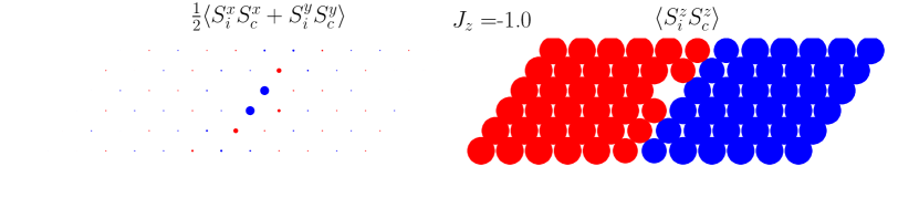
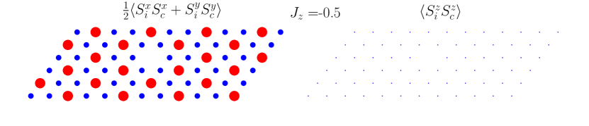
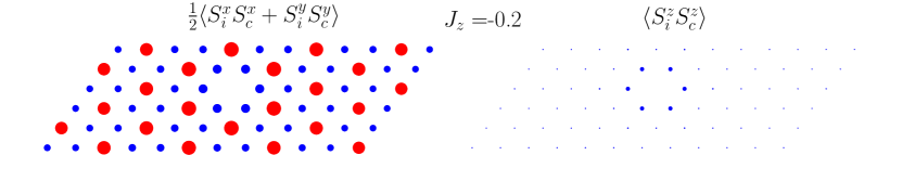
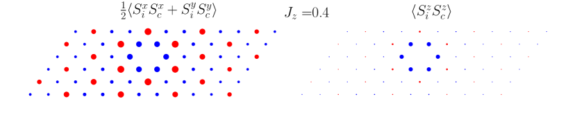
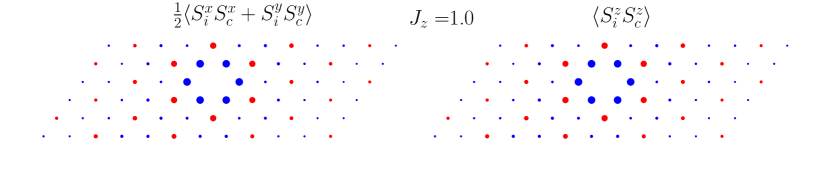
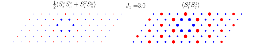
Figure 10: Real space correlation functions (measured with respect to a central site $c$) $\frac{1}{2}\langle S^{x}_{i}S^{x}_{c}+S^{y}_{i}S^{y}_{c}\rangle$ and $\langle S^{z}_{i}S^{z}_{c}\rangle$ for the triangular lattice in the $m=0$ ($S_{z}=0$) magnetization sector, at various representative $J_{z}$. The correlation function of the spin at a site with itself is not plotted, and is left empty. The size of the circles indicates the magnitude of the correlator and the color indicates the sign, blue being negative and red being positive.

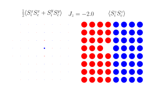
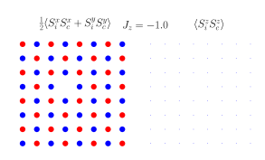
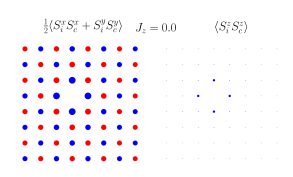
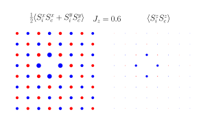
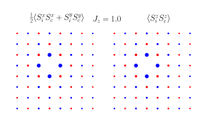
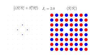
Figure 11: Real space correlation functions (measured with respect to a central site $c$) $\frac{1}{2}\langle S^{x}_{i}S^{x}_{c}+S^{y}_{i}S^{y}_{c}\rangle$ and $\langle S^{z}_{i}S^{z}_{c}\rangle$ for the $8\times 8$ square lattice cylinder in the $m=0$ ($S_{z}=0$) magnetization sector, at various representative $J_{z}$. The correlation function of the spin at a site with itself is not plotted, and is left empty. The size of the circles indicates the magnitude of the correlator and the color indicates the sign, blue being negative and red being positive.

Appendix G Tables

In this section, we list the tables that have been referred to in the main text in Sec. II and  IV.

$(L_{x},L_{y})$	$\frac{E_{|C\rangle}}{\#\text{bonds}}$	$\frac{E_{ED}}{\#\text{bonds}}$	$\#_{|C\rangle}$ $(N+1)$	$\#_{ED}$	$\langle\hat{S}^{z}_{i}\hat{S}^{z}_{j}\rangle_{|C\rangle}$ $(-\frac{1}{4}\frac{1}{N-1})$	$\langle\hat{S}^{z}_{i}\hat{S}^{z}_{j}\rangle_{ED}$	$\epsilon_{ij}\langle\hat{S}^{x}_{i}\hat{S}^{x}_{j}\rangle_{|C\rangle}$ $(\frac{1}{8}\frac{N}{N-1})$	$\epsilon_{ij}\langle\hat{S}^{x}_{i}\hat{S}^{x}_{j}\rangle_{ED}$
(2,2)/(4,1)	-0.25	-0.250000..	5	5	-1/12	-0.083333..	1/6	0.166666..
(4,2)	-0.25	-0.250000..	9	9	-1/28	-0.035714..	1/7	0.142857..
(6,2)	-0.25	-0.250000..	13	13	-1/44	-0.022727..	3/22	0.136364..
(4,4)	-0.25	-0.250000..	17	17	-1/60	-0.016666..	2/15	0.133333..
(6,4)	-0.25	-0.250000..	25	25	-1/92	-0.0108696	3/23	0.130435..
(8,4)	-0.25	-0.250000..	33	33	-1/124	-0.0080645	4/31	0.129032..

Table 1: Comparison of exact analytic results with exact diagonalization computations for the case of two-coloring. The results hold for both periodic and open boundary conditions.

Configuration	$2^{3/2}|D_{1}\rangle$	$2^{3/2}|D_{2}\rangle$	$2^{3/2}\Big{(}|D_{1}\rangle+|D_{2}\rangle\Big{)}$	$\sqrt{20}P_{S_{z}=0}|rbgrbg\rangle$	$\sqrt{20}P_{S_{z}=0}|rgbrgb\rangle$	$\frac{\sqrt{20}}{\omega^{2}-\omega}\Big{(}|rgbrgb\rangle-|rbgrbg\rangle\Big{)}$
$|\uparrow\uparrow\uparrow\downarrow\downarrow\downarrow\rangle$	0	0	0	1	1	0
$|\uparrow\uparrow\downarrow\downarrow\downarrow\uparrow\rangle$	0	0	0	1	1	0
$|\uparrow\downarrow\uparrow\downarrow\downarrow\uparrow\rangle$	$-1$	0	$-1$	$\omega^{2}$	$\omega$	$-1$
$|\downarrow\uparrow\uparrow\downarrow\downarrow\uparrow\rangle$	$+1$	0	$+1$	$\omega$	$\omega^{2}$	$+1$
$|\uparrow\uparrow\downarrow\downarrow\uparrow\downarrow\rangle$	0	$+1$	$+1$	$\omega$	$\omega^{2}$	$+1$
$|\uparrow\downarrow\uparrow\downarrow\uparrow\downarrow\rangle$	$+1$	$-1$	0	1	1	0
$|\downarrow\uparrow\uparrow\downarrow\uparrow\downarrow\rangle$	$-1$	0	$-1$	$\omega^{2}$	$\omega$	$-1$
$|\uparrow\uparrow\downarrow\uparrow\downarrow\downarrow\rangle$	0	$-1$	$-1$	$\omega^{2}$	$\omega$	$-1$
$|\uparrow\downarrow\uparrow\uparrow\downarrow\downarrow\rangle$	0	$+1$	$+1$	$\omega$	$\omega^{2}$	$+1$
$|\downarrow\uparrow\uparrow\uparrow\downarrow\downarrow\rangle$	0	0	0	1	1	0
$|\downarrow\downarrow\downarrow\uparrow\uparrow\uparrow\rangle$	0	0	0	1	1	0
$|\downarrow\downarrow\uparrow\uparrow\uparrow\downarrow\rangle$	0	0	0	1	1	0
$|\downarrow\uparrow\downarrow\uparrow\uparrow\downarrow\rangle$	$+1$	0	$+1$	$\omega$	$\omega^{2}$	$+1$
$|\uparrow\downarrow\downarrow\uparrow\uparrow\downarrow\rangle$	$-1$	0	$-1$	$\omega^{2}$	$\omega$	$-1$
$|\downarrow\downarrow\uparrow\uparrow\downarrow\uparrow\rangle$	0	$-1$	$-1$	$\omega^{2}$	$\omega$	$-1$
$|\downarrow\uparrow\downarrow\uparrow\downarrow\uparrow\rangle$	$-1$	$+1$	0	1	1	0
$|\uparrow\downarrow\downarrow\uparrow\downarrow\uparrow\rangle$	$+1$	0	$+1$	$\omega$	$\omega^{2}$	$+1$
$|\downarrow\downarrow\uparrow\downarrow\uparrow\uparrow\rangle$	0	$+1$	$+1$	$\omega$	$\omega^{2}$	$+1$
$|\downarrow\uparrow\downarrow\downarrow\uparrow\uparrow\rangle$	0	$-1$	$-1$	$\omega^{2}$	$\omega$	$-1$
$|\uparrow\downarrow\downarrow\downarrow\uparrow\uparrow\rangle$	0	0	0	1	1	0

Table 2: Amplitudes of dimer and three-coloring wavefunctions (and linear combinations) for all 20 Ising configurations in the $S_{z}=0$ sector for the six site chain with periodic boundary conditions. $\omega\equiv\exp(\frac{i2\pi}{3})$ is the cube root of unity.

References

- Giamarchi (2004) T. Giamarchi, Quantum Physics in One Dimension (Oxford University Press, 2004).
- Chakravarty et al. (1989) S. Chakravarty, B. I. Halperin, and D. R. Nelson, Phys. Rev. B 39, 2344 (1989).
- Huse and Elser (1988) D. A. Huse and V. Elser, Phys. Rev. Lett. 60, 2531 (1988).
- Jolicoeur and Le Guillou (1989) T. Jolicoeur and J. C. Le Guillou, Phys. Rev. B 40, 2727 (1989).
- Singh and Huse (1992) R. R. P. Singh and D. A. Huse, Phys. Rev. Lett. 68, 1766 (1992).
- Bernu et al. (1992) B. Bernu, C. Lhuillier, and L. Pierre, Phys. Rev. Lett. 69, 2590 (1992).
- Capriotti et al. (1999) L. Capriotti, A. E. Trumper, and S. Sorella, Phys. Rev. Lett. 82, 3899 (1999).
- Kadowaki et al. (1995) H. Kadowaki, H. Takei, and K. Motoya, Journal of Physics: Condensed Matter 7, 6869 (1995).
- Ishii et al. (2011) R. Ishii, S. Tanaka, K. Onuma, Y. Nambu, M. Tokunaga, T. Sakakibara, N. Kawashima, Y. Maeno, C. Broholm, D. P. Gautreaux, J. Y. Chan, and S. Nakatsuji, EPL (Europhysics Letters) 94, 17001 (2011).
- Shirata et al. (2012) Y. Shirata, H. Tanaka, A. Matsuo, and K. Kindo, Phys. Rev. Lett. 108, 057205 (2012).
- Bethe (1931) H. Bethe, Zeitschrift für Physik 71, 205 (1931).
- Guan et al. (2013) X.-W. Guan, M. T. Batchelor, and C. Lee, Rev. Mod. Phys. 85, 1633 (2013).
- Karabach et al. (1997) M. Karabach, G. Müller, H. Gould, and J. Tobochnik, Computers in Physics 11, 36 (1997).
- Karbach et al. (1998) M. Karbach, K. Hu, and G. Müller, Computers in Physics 12, 565 (1998).
- Levkovich-Maslyuk (2016) F. Levkovich-Maslyuk, Journal of Physics A: Mathematical and Theoretical 49, 323004 (2016).
- Majumdar and Ghosh (1969) C. K. Majumdar and D. K. Ghosh, Journal of Mathematical Physics 10, 1388 (1969).
- Affleck et al. (1987) I. Affleck, T. Kennedy, E. H. Lieb, and H. Tasaki, Phys. Rev. Lett. 59, 799 (1987).
- Shastry and Sutherland (1981) B. S. Shastry and B. Sutherland, Physica B+C 108, 1069 (1981).
- Kitaev (2006) A. Kitaev, Annals of Physics 321, 2 (2006).
- Changlani et al. (2018) H. J. Changlani, D. Kochkov, K. Kumar, B. K. Clark, and E. Fradkin, Phys. Rev. Lett. 120, 117202 (2018).
- Changlani et al. (2019) H. J. Changlani, S. Pujari, C.-M. Chung, and B. K. Clark, Physical Review B 99, 104433 (2019).
- Richter et al. (2004) J. Richter, J. Schulenburg, and A. Honecker, “Quantum magnetism in two dimensions: From semi-classical néel order to magnetic disorder,” in Quantum Magnetism, edited by U. Schollwöck, J. Richter, D. J. J. Farnell, and R. F. Bishop (Springer Berlin Heidelberg, Berlin, Heidelberg, 2004) pp. 85–153.
- Okuma et al. (2019) R. Okuma, D. Nakamura, T. Okubo, A. Miyake, A. Matsuo, K. Kindo, M. Tokunaga, N. Kawashima, S. Takeyama, and Z. Hiroi, Nature communications 10, 1 (2019).
- Schnack et al. (2020) J. Schnack, J. Schulenburg, A. Honecker, and J. Richter, Phys. Rev. Lett. 125, 117207 (2020).
- Derzhko et al. (2020) O. Derzhko, J. Schnack, D. V. Dmitriev, V. Y. Krivnov, and J. Richter, The European Physical Journal B 93, 161 (2020).
- Momoi and Suzuki (1992) T. Momoi and M. Suzuki, Journal of the Physical Society of Japan 61, 3732 (1992).
- Chubukov and Golosov (1991) A. V. Chubukov and D. I. Golosov, Journal of Physics: Condensed Matter 3, 69 (1991).
- Pal et al. (2020) S. Pal, A. Mukherjee, and S. Lal, Journal of Physics: Condensed Matter 32, 165805 (2020).
- White (1992) S. R. White, Phys. Rev. Lett. 69, 2863 (1992).
- Fishman et al. (2020) M. Fishman, S. R. White, and E. M. Stoudenmire, “The ITensor software library for tensor network calculations,” (2020), arXiv:2007.14822 .
- (31) For any operator that commutes with the Hamiltonian , if is an eigenstate, , then it also follows that and thus is an eigenstate as well. In our case, is the projection operator . The opposite however does not follow, i.e. does not imply .
- Lieb and Mattis (1962) E. Lieb and D. Mattis, Journal of Mathematical Physics 3, 749 (1962).
- Bishop et al. (2017) R. F. Bishop, P. H. Li, R. Zinke, R. Darradi, J. Richter, D. Farnell, and J. Schulenburg, Journal of Magnetism and Magnetic Materials 428, 178 (2017).
- Cuccoli et al. (2003) A. Cuccoli, T. Roscilde, V. Tognetti, R. Vaia, and P. Verrucchi, Phys. Rev. B 67, 104414 (2003).
- (35) C. Lhuillier arXiv:cond-mat/0502464v1 (unpublished).
- White and Chernyshev (2007) S. R. White and A. L. Chernyshev, Phys. Rev. Lett. 99, 127004 (2007).
- Sellmann et al. (2015) D. Sellmann, X.-F. Zhang, and S. Eggert, Physical Review B (R) 91, 081104 (2015).
- Wang et al. (2009) F. Wang, F. Pollmann, and A. Vishwanath, Physical Review Letters 102, 017203 (2009).
- Jiang et al. (2009) H. Jiang, M. Weng, Z. Weng, D. Sheng, and L. Balents, Physical Review B (R) 79, 020409 (2009).
- Heidarian and Paramekanti (2010) D. Heidarian and A. Paramekanti, Physical review letters 104, 015301 (2010).
- Pujari et al. (2016) S. Pujari, T. C. Lang, G. Murthy, and R. K. Kaul, Physical Review Letters 117, 086404 (2016).
- Alicea et al. (2009) J. Alicea, A. V. Chubukov, and O. A. Starykh, Physical Review Letters 102, 137201 (2009).
- Yamamoto et al. (2014) D. Yamamoto, G. Marmorini, and I. Danshita, Phys. Rev. Lett. 112, 127203 (2014).
- Caspers et al. (1984) W. J. Caspers, K. M. Emmett, and W. Magnus, Journal of Physics A: Mathematical and General 17, 2687 (1984).
- Chertkov and Clark (2018) E. Chertkov and B. K. Clark, Physical Review X 8, 031029 (2018).
- Yu et al. (2005) R. Yu, T. Roscilde, and S. Haas, Phys. Rev. Lett. 94, 197204 (2005).
- Wang and Sandvik (2006) L. Wang and A. W. Sandvik, Phys. Rev. Lett. 97, 117204 (2006).
- Sandvik (2002) A. W. Sandvik, Phys. Rev. B 66, 024418 (2002).
- Kato et al. (2000) K. Kato, S. Todo, K. Harada, N. Kawashima, S. Miyashita, and H. Takayama, Phys. Rev. Lett. 84, 4204 (2000).
- Changlani et al. (2013) H. J. Changlani, S. Ghosh, S. Pujari, and C. L. Henley, Phys. Rev. Lett. 111, 157201 (2013).
- Ghosh et al. (2015) S. Ghosh, H. J. Changlani, and C. L. Henley, Phys. Rev. B 92, 064401 (2015).
- He and Chen (2015) Y.-C. He and Y. Chen, Phys. Rev. Lett. 114, 037201 (2015).
- Läuchli and Moessner (2015) A. M. Läuchli and R. Moessner, ArXiv e-prints (2015), arXiv:1504.04380 [cond-mat.quant-gas] .
- Kumar et al. (2016) K. Kumar, H. J. Changlani, B. K. Clark, and E. Fradkin, Phys. Rev. B 94, 134410 (2016).
- Lee et al. (2020a) K. Lee, R. Melendrez, A. Pal, and H. J. Changlani, Phys. Rev. B 101, 241111 (2020a).
- Lee et al. (2020b) K. Lee, A. Pal, and H. J. Changlani, “Frustration-induced emergent hilbert space fragmentation,” (2020b), arXiv:2011.01936 [cond-mat.str-el] .