The TW Hya Rosetta Stone Project III: Resolving the Gaseous Thermal Profile of the Disk

Abstract

The thermal structure of protoplanetary disks is a fundamental characteristic of the system that has wide reaching effects on disk evolution and planet formation. In this study, we constrain the 2D thermal structure of the protoplanetary disk TW Hya structure utilizing images of seven CO lines. This includes new ALMA observations of ${}^{12}\textrm{CO}$ $J$=2-1 and $\textrm{C}^{18}\textrm{O}$ $J$=2-1 as well as archival ALMA observations of ${}^{12}\textrm{CO}$ $J$=3-2, ${}^{13}\textrm{CO}$ $J$=3-2, 6-5, $\textrm{C}^{18}\textrm{O}$ $J$= 3-2, 6-5. Additionally, we reproduce a Herschel observation of the HD $J$=1-0 line flux, the spectral energy distribution, and utilize a recent quantification of CO radial depletion in TW Hya. These observations were modeled using the thermo-chemical code RAC2D, and our best fit model reproduces all spatially resolved CO surface brightness profiles. The resulting thermal profile finds a disk mass of 0.025 $\textrm{M}_{\odot}$ and a thin upper layer of gas depleted of small dust with a thickness of $\sim$1.2% of the corresponding radius. Using our final thermal structure, we find that CO alone is not a viable mass tracer as its abundance is degenerate with the total $\textrm{H}_{2}$ surface density. Different mass models can readily match the spatially resolved CO line profiles with disparate abundance assumptions. Mass determination requires additional knowledge and, in this work, HD provides the additional constraint to derive the gas mass and support the inference of CO depletion in the TW Hya disk. Our final thermal structure confirms the use of HD as a powerful probe of protoplanetary disk mass. Additionally, the method laid out in this paper is an employable strategy for extraction of disk temperatures and masses in the future.

1 Introduction

The radial and vertical (2D) thermal profile of a gaseous protoplanetary disk is difficult to uncover but has wide reaching effects on the physics, chemistry, and thus the planet formation potential of a disk. Further, temperature is often essential for estimation of other fundamental disk properties, such as the local sound speed and disk mass (Bergin & Williams, 2017). Any physical process that relies on sound speed will also be affected by temperature. Turbulent viscosity, as one example, relies on sound speed and plays an important role in the transportation and redistribution of disk material (Shakura & Sunyaev, 1973). The vertical density structure, in addition to the radial dependence, gives rise to the flaring of the disk, and is highly dependent on the thermal structure (Kenyon & Hartmann, 1995). In turn, the level of flaring sets the angle of incidence to stellar irradiation, producing strong vertical thermal gradients that lead to density profiles that deviate significantly from the derived Gaussian density profiles from assuming a vertically isothermal disk (Aikawa et al., 2002; Gorti et al., 2011; Woitke et al., 2009).

Temperature is also a determinate parameter to chemical processes. The gas temperature influences the rate of gas-phase exothermic reactions and, in particular, reactions that possess a significant activation barrier. Further, the midplane temperature controls the balance between gas-phase deposition and sublimation and thus the relative spatial composition of ices. For example, $\textrm{H}_{2}\textrm{O}$ freezes out at dust temperatures lower than $\approx$ 120 K - 170 K (Fraser et al., 2001; Bergin & Cleeves, 2018), while CO freezes out below $\sim$21-25 K in TW Hya, (Bisschop et al., 2006; Fayolle et al., 2016; Schwarz et al., 2016; Zhang et al., 2017). Thus the gas/ice transition or snowline for water and CO is set by the thermal structure with water close to the star and CO at greater distances. Temperature-dependent snowlines are theorized to potentially be favorable sites for planet formation (Hayashi, 1981; Stevenson & Lunine, 1988; Zhang et al., 2015; Schoonenberg & Ormel, 2017). Further, across various snowlines of key elemental carriers, the relative chemical composition of the disk changes the gas/solid state balance of these carriers, which will directly influence the chemical composition of planetary atmospheres or cores at birth (e.g. C/O ratio, Öberg et al., 2011; Öberg & Bergin, 2016).

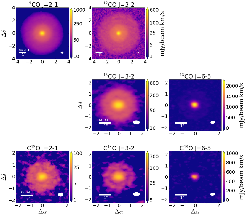
Figure 1: Integrated emission maps of TW Hya in ${}^{12}\textrm{CO}$ J=2-1, 3-2, ${}^{13}\textrm{CO}$ J=3-2, 6-5, $\textrm{C}^{18}\textrm{O}$ J=2-1, 3-2, and 6-5. The beam size is in the bottom right of each image. All lines of CO with the exception of the 6-5 lines are shown in log scale to amplify features. The 6-5 lines are shown on a linear scale as they have one peak and no substructure to highlight. The contour lines shown in ${}^{13}\textrm{CO}$ 3-2 and $\textrm{C}^{18}\textrm{O}$ 6-5 are overlain on ${}^{12}\textrm{CO}$ 2-1 to compare emission region sizes.

Table 1: ALMA Observations Summary

						$\sigma^{b}$	v${}_{\sigma}^{c}$	$\rm I_{peak}^{d}$	$\rm F_{\textrm{line}}^{e}$
Program ID	P.I.	Species and	Frequency	$\rm E_{\textrm{up}}^{a}$	Beam [PA]	(mJy/	(km/	(mJy/bm	(Jy
		Transition	(GHz)	(K)	(AU $\times$ AU) [∘]	bm)	s)	km/s)	km/s)
2016.1.00311.S	I. Cleeves	${}^{12}\textrm{CO}$ J=2-1	230.538	16.6	22 $\times$ 16 [89.02]	3.9	0.56	828	17.8
2015.1.00686.S	S. Andrews	${}^{12}\textrm{CO}$ J=3-2	345.795	33.2	8.3 $\times$ 7.7 [-74.96]	1.7	0.25	541	43.2
2016.1.00629.S	I. Cleeves
2012.1.00422.S	E. Bergin	${}^{13}\textrm{CO}$ J=3-2	330.587	15.9	30 $\times$ 18 [88.15]	9.2	0.09	574	4.35
2012.1.00422.S	E. Bergin	${}^{13}\textrm{CO}$ J=6-5	661.067	111.1	23 $\times$ 14 [-84.84]	56	0.11	2248	8.21
2016.1.00311.S	I. Cleeves	$\textrm{C}^{18}\textrm{O}$ J=2-1	219.560	15.8	24 $\times$ 18 [87.65]	3.2	0.10	66	0.57
2012.1.00422.S	E. Bergin	$\textrm{C}^{18}\textrm{O}$ J=3-2	329.331	31.6	30 $\times$ 18 [88.62]	12	0.11	252	1.16
2012.1.00422.S	E. Bergin	$\textrm{C}^{18}\textrm{O}$ J=6-5	658.553	110.6	23 $\times$ 14 [-79.98]	77	0.09	973	1.56

Temperature is also essential in estimating one of the most fundamental properties of a protoplanetary disk: its mass. Assuming a constant mass ratio between gas and dust and a dust mass opacity, sub-mm thermal continuum emission is generally used as an approximate tracer for the gas mass (Bergin & Williams, 2017). However, this estimation is subject to large uncertainty as grain evolution alters the dust opacity, both spatially and temporally; compounding the issue, the growth to pebble sizes and larger renders a large fraction of the solids inemissive at sub-mm wavelengths and essentially undetectable (Andrews, 2020). CO emission provides an alternative method to estimate the gas mass as CO has long been used as a tracer of $\textrm{H}_{2}$ mass in molecular clouds. However, the conversion of line emission to column density requires a prior knowledge of the temperature, CO distribution, and opacity to account for the fact that observations generally only sample the upper state column of one rotational state. The CO abundance relative to $\textrm{H}_{2}$ remains relatively consistent throughout the dense ISM at approximately $10^{-4}$ relative to $\textrm{H}_{2}$ (Frerking et al., 1982; Lacy et al., 1994; Bergin & Williams, 2017; Lacy et al., 2017). In protoplanetary disks, however, CO appears to be physically depleted and such depletion varies not only disk by disk (Ansdell et al., 2016; Miotello et al., 2017; Long et al., 2017), but radially (Zhang et al., 2019, 2020a), and possibly temporally due to chemical and physical evolution (Reboussin et al., 2015; Bosman et al., 2018; Cleeves et al., 2018; Eistrup et al., 2018; Krijt et al., 2018; Schwarz et al., 2019; Zhang et al., 2020b). All of these factors complicate the use of CO to provide a reliable estimate of the total gas mass.

HD is a promising mass tracer, as the ratio of HD/$\textrm{H}_{2}$ is well calibrated via measurements of the atomic D/H ratio (Linsky, 1998). However the conversion of emission of HD to mass is strongly temperature sensitive for typical temperatures between 20–50 K; this is due to the first rotational state (J = 1-0) having an $\rm E_{\rm up}$ equal to 128.5 K above the ground (Bergin et al., 2013; Bergin & Williams, 2017; Kama et al., 2020). A well constrained disk mass derived using HD, can only be determined if an accurate thermal structure is available (Trapman et al., 2017; Kama et al., 2020).

Given the wide reaching impact of the thermal structure of a protoplanetary disk, it has long been a property sought after. Before the advent of the Atacama Large (sub-)Millimeter Array (ALMA), the spectral energy distribution (SED) and spatially unresolved gas observations provided the best available constraints for most disks. One of the first attempts to uncover a thermal structure with single dish observations was van Zadelhoff et al. (2001), which utilized isotopologues of CO, HCO⁺, and HCN. By measuring the ratios of flux, they extrapolated densities and temperatures from which that flux originated. But with unresolved observations, spatial information becomes degenerate as each of the isotopologues can be sensitive to different radial and vertical layers in the disk (Gorti et al., 2011; Zhang et al., 2017; Woitke et al., 2019). Spectrally resolved observations of isotopologues have already been illuminating, shedding light onto the thermal profiles of a handful of disks, i.e. Fedele et al. (2016), which utilized both spectrally resolved and unresolved lines of high-$J$ CO to extract thermal profiles of disks. While spatially unresolved, the spectrally resolved observations still can extract spatial information from the Keplerian rotation, if the disk inclination is known.

Spatially resolved observations allow for measurements of column densities and temperature information at different disk radii (Bruderer et al., 2012; Rosenfeld et al., 2013; Schwarz et al., 2016; Zhang et al., 2017; Pinte et al., 2018) providing finer constraints in a forward modeling approach. Kama et al. (2016a) was one of the first to derive a thermal structure using a spatially resolved line, using CO 3-2 towards TW Hya. This resolved line in addition to much of the CO ladder produced improvements to the understanding of the TW Hya thermal profile. Towards IM Lup, Pinte et al. (2018) observed the 2-1 transition of ${}^{12}\textrm{CO}$, ${}^{13}\textrm{CO}$, and $\textrm{C}^{18}\textrm{O}$ and directly extrapolated T_gas from spatially resolved optically thick lines, independent of any modeling.

The thermal structure of TW Hya has been probed using its SED in concert with a large array of spatially unresolved lines including various transitions of CO, HCO⁺, and H₂O (van Zadelhoff et al., 2001; Gorti et al., 2011; Zhang et al., 2017; Woitke et al., 2019). Often these thermal profiles were empirically derived using these observations. With new thermo-chemical models that take into account radiative transfer and chemical evolution, the disk thermal structure can be derived using a forward modeling approach by reproducing observations (Woitke et al., 2019) including spatially resolved lines providing finer insight into radial structure (Kama et al., 2016a). The goals of this paper are to lay out a new approach to uncover a gaseous protoplanetary disk thermal profile by utilizing multiple spatially-resolved observations. Using a thermo-chemical code, we aim to reproduce seven spatially-resolved CO line observations towards the class II, nearby (60pc; Gaia Collaboration et al., 2018; Bailer-Jones et al., 2018), face-on TW Hya disk. It is worth noting that we do not seek to reproduce scattered light nor continuum observations. While these observations provide additional constraints on the temperature structure (more directly on the dust temperature and indirectly on gas temperature), a detailed dust model would require further assumptions on how dust properties vary with radius (Huang et al., 2018), as well as assumptions on dust scattering, which add uncertainty in dust temperature determinations (Zhu et al., 2019). Such simulated observations would be non-trivial with our current model, and the goal of this paper is to uncover the broader gaseous thermal profile and mass. While continuum and scattered light images provide insight into deviations from a smooth density distribution, that information may not translate into an effect on the gas density and temperature.

The present study uses data from the TW Hya Rosetta Stone Project (PI: Cleeves) along with other archival data sets. The complete set of observations, including the CO and isotopologue maps from Schwarz et al. (2016) and Huang et al. (2018), span a wide range of optical depths, thereby tracing both the vertical and radial temperature simultaneously when observations are spatially resolved, in the case for optically thick molecules. Molecules that turn out to be optically thin will provide column density information. Additionally, we seek to reproduce the HD flux measured with Herschel and the SED of the disk.

We detail our ALMA observations in Section 2 and our modeling procedure in Section 3. In Section 4 we explore our best fit thermal model to investigate possible model degeneracies. Comparisons to other models and the future of HD observations are explored in Section 5, and we summarize our findings in Section 6.

2 Observations

We present new observations of ${}^{12}\textrm{CO}$ 2-1 and $\textrm{C}^{18}\textrm{O}$ 2-1 taken as a part of the Rosetta collaboration. Archival ALMA data were also used for ${}^{12}\textrm{CO}$ 3-2, $\textrm{C}^{18}\textrm{O}$ 3-2, 6-5, and ${}^{13}\textrm{CO}$ 3-2, 6-5. The archival HD 1-0 flux measurement from Herschel and SED fluxes from the literature were also used. A summary of all observations can be found in Table 1. Using bettermoments (Teague & Foreman-Mackey, 2018), moment zero maps were calculated for each of the CO observations described below and are presented in Figure 1. Each moment zero map was then azimuthally averaged producing the radial emission profiles. These radial profiles provided the constraints that we used below to determine the 2D thermal structure of TW Hya.

2.1 CO Observations from TW Hya Rosetta Project

We report new observations of ${}^{12}\textrm{CO}$ 2-1 and $\textrm{C}^{18}\textrm{O}$ 2-1 as part of the program 2016.1.00311.S (PI Cleeves). The compact observations (baselines down to 15 m) were obtained on December 16, 2016 in configuration C43-3 for a total on-source integration time of 81 minutes. The extended observations (baselines up to 1124 m) were carried out on May 5 and 7, 2017 in C43-6 with an on source integration time of 25 minutes. The data were calibrated by the CASA pipeline McMullin et al. (2007). For the extended observations, J1058+0133 and J1037-2934 were used as bandpass calibrators, J1107-4449 as the flux calibration, and J1037-2934 as the phase calibrator. For the compact observations, J1037-2934 was used for bandpass, flux, and phase calibration. We performed one additional round of phase self calibration on each of the extended and compact observations independently using CASA version 4.5.0. For the self calibration we adopted a solution interval of 30 seconds and averaged both polarizations. Spectral windows were not averaged in the self calibration step, and the solutions were mapped to the individual spectral windows.

Each data cube was first centered to the same central coordinate, then the continuum was subtracted from the line observations in the uv plane using the CASA routine uvcontsub. The continuum subtracted long and short baselines were then combined using the method concat where the spectral windows that excluded the lines were manually specified. The images were produced in CASA version 4.6.12 using tclean, with Briggs weighting and a robust parameter of 0.5. The final spectral resolution of CO and $\textrm{C}^{18}\textrm{O}$ were 246.08 kHz and 73.24 kHz respectively. The $\textrm{C}^{18}\textrm{O}$ restoring beam had FWHM dimensions of $0.^{\prime\prime}40\times 0.^{\prime\prime}30$ and ${}^{12}\textrm{CO}$ had $0.^{\prime\prime}37\times 0.^{\prime\prime}28$.

2.2 Archival CO Data

The ${}^{12}\textrm{CO}$ $J$ = 3-2 analysis and imaging procedures are reported in Huang et al. (2018) and the ${}^{13}\textrm{CO}$ $J$ = 3-2, 6-5 and $\textrm{C}^{18}\textrm{O}$ $J$ = 3-2, 6-5 observations are described in Schwarz et al. (2016), and not repeated here. We utilize their final data reduction and images.

2.3 Spatially Unresolved Observations:
HD Flux and SED

HD J=1-0 was observed using Herschel and the observed total integrated flux was $6.3(\pm 0.7)\times 10^{-18}$ $\textrm{W/m}^{2}$ (Bergin et al., 2013). The line is spatially unresolved, thus we only use the integrated line flux to compare the models.

TW Hya is one of the most thoroughly observed protoplanetary disks in the literature, with a well-characterized spectral energy distribution (SED). The main purpose of the SED is to constrain the thermally coupled small dust population. Data points for the SED were taken from Cleeves et al. (2015), which in turn used individual photometric measurements from the literature (Weintraub et al., 1989a, 2000; Mekkaden, 1998; Cutri et al., 2003; Hartmann et al., 2005; Low et al., 2005; Thi et al., 2010; Andrews et al., 2012; Qi et al., 2004; Wilner et al., 2000, 2003).

3 Modeling: RAC2D

We create a thermo-chemical model of the TW Hya disk that takes into account the gas and dust structure while simultaneously computing the temperature and chemical structure throughout the disk over time. Simulated observations are derived from the output model and compared to spatially-resolved line observations, as well as the SED and HD line flux. We use the time-dependent thermo-chemical code RAC2D (Du & Bergin, 2014). A brief description of the physical model follows; a higher-level detailed description of the code can be found in the aforementioned paper.

3.1 Physical Structure

Our model consists of three mass components: gas, a small dust ($\leq$ µm) population, and a large dust ($\leq$ mm) population. Each population is described by a global surface density distribution (Lynden-Bell & Pringle, 1974) which has been widely used in modeling protoplanetary disks:

$$\Sigma(r)=\Sigma_{c}\left(\frac{r}{r_{c}}\right)^{-\gamma}\exp{\left[-\left(\frac{r}{r_{c}}\right)^{2-\gamma}\right]}$$ (1)

$r_{c}$ is the characteristic radius at which the surface density is $\Sigma_{c}$ and $\gamma$ is the power-law index that describes the radial behavior of the surface density. Each dust population follows an MRN grain size distribution $n(a)\propto a^{-3.5}$ (Mathis et al., 1977) . The gas and small dust are spatially coupled and exist out to 200 AU (van Boekel et al., 2017; Huang et al., 2018) and possess a scale height that is related to a critical radius (defined below). We assume that the large dust population is settled in the midplane and extends less than 100 AU (Andrews et al., 2010). This reduced scale height approximates and represents the impact of dust evolution and pebble sedimentation to the midplane (Birnstiel et al., 2012; Krijt et al., 2016). The specific values for our TW Hya model are constrained by observation and detailed in the next section.

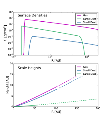
Figure 2: The surface density (top) and the scale heights (bottom) of each component of our disk model. The exponential taper seen added to the surface densities at 60 AU for the large dust and 104 AU for the small dust and gas components. The location at which dashed line starts for the scale height also corresponds to where the exponential taper for that population begins, corresponding to a significant decrease in density.

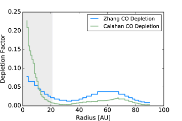
Figure 3: The final radial depletion profile (green) as motivated by the depletion profiles derived in Zhang et al. (2019) (blue). CO was depleted radially according to the above factor at the beginning of the thermo-chemical calculation. The transparent grey corresponds to the beamsize of the $\textrm{C}^{18}\textrm{O}$ 2-1 observation.

RAC2D is equipped with an exponential taper added to the surface density profile both in the inner and outer disk regions. This allows for more flexibility in the position of the exponential taper. If $r_{c}$ is defined to be larger than the gas component (which would result in a flatter disk) an exponential taper can still be added. If we were to only use Equation 1, and required a large $r_{c}$ value, there would be an abrupt cut-off at the user-defined outer radius. $r_{exp}$ defines at what radius the exponential taper begins, and $r_{s}$ describes the strength of that taper:

$\Sigma^{\prime}(r)=\Sigma(r)e^{(r-r_{\rm exp_{\rm in}})/r_{s_{in}}}$, if $r<r_{\rm exp_{\rm in}}$

$\Sigma^{\prime}(r)=\Sigma(r)e^{-(r-r_{\rm exp_{\rm out}})/r_{\rm s_{out}}}$, if $r>r_{\rm exp_{\rm out}}$

A density profile for the gas and dust populations is derived from the surface density profile and a scale height:

$$\rho(r,z)=\frac{\Sigma(r)}{\sqrt{2\pi}h(r)}\exp{\left[-\frac{1}{2}\left(\frac{z}{h(r)}\right)^{2}\right]}$$ (2)

$$h=h_{c}\left(\frac{r}{r_{c}}\right)^{\Psi}$$ (3)

Where $h_{c}$ is the scale height at the characteristic radius, and $\Psi$ is a power-law index that characterizes the flaring of the disk structure. The final surface densities and scale heights for each component in our model is seen in Figure 2. In the surface density plot, we show that although all of our components (gas, small dust, and large dust) have a $\rm r_{c}$ value equal to 400 AU, they exponentially drop off at their given $\rm r_{exp_{out}}$.

3.2 Dust and Gas Temperatures

After initializing RAC2D with a model density structure for each population, the code computes a dust and gas temperature. The determination of dust and gas temperature is an iterative process, allowed to change over time due to the evolving chemical composition. For the gas-phase chemistry, we adopt the reaction rates from the UMIST database (Woodall et al., 2007), with additional rates considering the self-shielding of CO, $\textrm{H}_{2}$, $\textrm{H}_{2}\textrm{O}$, and OH, dust grain surface chemistry driven by temperature, UV, cosmic rays, and two-body chemical reactions on dust grain surfaces (see references given by Du & Bergin, 2014). Chemical processes also provide heating or cooling to the surrounding gas. That, along with stellar and interstellar radiation drive the thermal gas structure. Our study explores models that account for 1 Myr of chemical evolution. Although the age of TW Hya is estimated to be 5-10 Myr (Debes et al., 2013), our assumed depletion profile for CO (Section 3.3) encapsulates the effects of earlier chemical evolution of CO. We are essentially modeling the thermal physics and chemistry after that evolution has occurred. Finally, at the end of a given run we extract the dust and gas thermal profiles and SED profile.

Simulated line images for CO, ${}^{13}\textrm{CO}$, $\textrm{C}^{18}\textrm{O}$, and HD are necessary for our comparison to observations. We do not model isotopologue fractionation in this chemical network, as fractionation of CO is not significant in a massive disk like TW Hya (Miotello et al., 2014) . Thus, we compute ${}^{13}\textrm{CO}$ and $\textrm{C}^{18}\textrm{O}$ abundances based on ISM ratios of CO/${}^{13}\textrm{CO}$ = 69 and CO/$\textrm{C}^{18}\textrm{O}$ = 570 (Wilson, 1999). We then apply the depletion profile to each CO line. The HD abundance (see Table 2) remains constant. Given these abundances and the local gas temperature, RAC2D computes line images using a ray-tracing technique. We then manually convolve these simulated observations with the corresponding ALMA beam to make direct comparisons to data. Our HD 1-0 observations are spatially and spectrally unresolved, thus to recreate unresolved integrated flux measurements, we convolve our model HD line over a gaussian corresponding to the velocity resolution of the Herschel PACS instrument: $\sim$300 ${\rm km\,s^{-1}}$ (Poglitsch et al., 2010).

The SED is created by RAC2D by counting the number of photons over a range of frequencies that interact with the disk and would fall within a given range of sight lines. Thus photons directly emitted from the star are not accounted for, a design motivated by computational efficiency. To create the final SED the input stellar blackbody of TW Hya (stellar mass = 0.8 $\textrm{M}_{\odot}$ and T${}_{\textrm{eff}}$ $\approx$ 3400K) is added to the result produced by RAC2D.

Table 2: Initial Chemical Abundances for Final Model

	Abundance Relative to Total
	Hydrogen Nuclei
$\textrm{H}_{2}$	$5\times 10^{-1}$
HD	$2\times 10^{-5}$
He	0.09
CO*	$1.04\times 10^{-4}$
N	$7.5\times 10^{-5}$
$\textrm{H}_{2}\textrm{O (ice)}$	$1.8\times 10^{-4}$
S	$8\times 10^{-8}$
Si+	$8\times 10^{-9}$
Na+	$2\times 10^{-8}$
Mg+	$7\times 10^{-9}$
Fe+	$3\times 10^{-9}$
P	$3\times 10^{-9}$
F	$2\times 10^{-8}$
Cl	$4\times 10^{-9}$

Note. — *CO has an imposed radial depletion profile as shown in Figure 3

Table 3: Gas and Dust Population Parameters: Ranges and Initial Values

	Gas	Small Dust	Definition
		($5\times 10^{-3}$ - 1 $\micron$)
Mass ($\textrm{M}_{\odot}$)	0.01 - [0.05] - 0.06	$2.5\times 10^{-5}-[1\times 10^{-4}]-5\times 10^{-4}$	Total Mass
$\Psi$	0.8 - [1.2] - 1.6	0.8 - [1.2] - 1.6	Flaring Parameter
$\gamma$	0.5 - [.75] - 1.1	0.5 - [.75] - 1.1	Surface Density Power-Index
$\textrm{h}_{c}$	8.4 - [42] - 84	8.4 - [42] - 84	Characteristic Height
$r_{{\rm exp}_{\rm out}}$	60 - [104] - 200	60 - [104] - 200	Exponential Drop-off Radius in the Outer Disk
$r_{{\rm s}_{\rm out}}$	70.7	70.7	Exponential Drop-off Strength in the Outer Disk
$r_{{\rm exp}_{\rm in}}$	2	3.5	Exponential Drop-off Radius at the Inner Disk
$r_{{\rm s}_{\rm in}}$	0.1	0.5	Exponential Drop-off Strength at the Inner Disk
$r_{in}$ (AU)	0.1	0.5	Inner Radius Cut-off
$r_{out}$ (AU)	200	200	Outer Radius Cut-off
$\textrm{r}_{c}$	400	400	Characteristic Radius

Note. — This table shows the range of parameter space explored in each variable of our thermo-chemical model, with the initial value in brackets. Since the parameter values for the larg dust do not significantly impact the thermal structure, we do not explore variations in the equivalent parameters in the large dust component and keep these fixed to the Zhang et al. values (see Table 4). All length values are in units of AU.

Table 4: Gas and Dust Population Parameters: Final Model Values

	Gas	Small Dust	Large Dust
		($5\times 10^{-3}$ - 1 $\micron$)	($5\times 10^{-3}$ - $1\times 10^{3}$ $\micron$)
Mass ($\textrm{M}_{\odot}$)	0.025	$1.0\times 10^{-4}$	$4.0\times 10^{-4}$
$\Psi$	1.1	1.2	1.2
$\gamma$	0.75	0.75	1.0
${\rm h}_{c}$	42	42	8.4
$r_{{\rm exp}_{\rm out}}$	104	104	60
$r_{{\rm s}_{\rm out}}$	70.7	70.7	10
$r_{{\rm exp}_{\rm in}}$	2	3.5	N/A
$r_{{\rm s}_{\rm in}}$	0.1	0.5	N/A
$r_{in}$	0.1	0.5	1
$r_{out}$	200	200	200
${\rm r}_{c}$	400	400	400

Note. — Final values of the TW Hya model that reproduces the CO, HD, and SED observations. All length values are in units of AU.

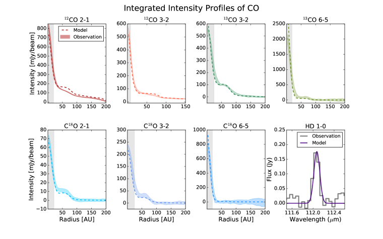
Figure 4: Integrated radial intensity profiles of CO and its isotopologues ${}^{13}\textrm{CO}$ and $\textrm{C}^{18}\textrm{O}$. The solid lines are from observations from ALMA (see Table 1) and the dashed lines are from our best-fit model, and each observation’s beam is shown in the filled region. The thermal profile that produced this best match to the observation is shown in Figure 6.

3.3 Initial Parameter Setup of TW Hya

We set out to create a model which, given certain initial parameters and constraints for the disk physical state, produces a gas thermal profile that can reproduce the spatially resolved CO observations and other constraints. Our initial parameters are taken from Zhang et al. (2019) who compiled the most up-to-date constraints on disk parameters from the literature: Brickhouse et al. (2010); Andrews et al. (2012); van Boekel et al. (2017); Gaia Collaboration et al. (2018); Huang et al. (2018). A table of source information is found in Table 3 of Zhang et al. (2019). For initial chemical abundances, we adopt values given in Table 2 motivated by Du & Bergin (2014) and Zhang et al. (2019). The disk inclination used is 6^∘, as past studies of TW Hya tend to use a range of inclination values between 5-7^∘ (Qi et al., 2004; Andrews et al., 2012; Huang et al., 2018)

In this study, we begin with a radial CO abundance profile motivated by Zhang et al. (2019), which calculated two depletion profiles, one for ${}^{13}\textrm{CO}$ and one for $\textrm{C}^{18}\textrm{O}$. They were calculated to fit the isotopologue observations. The depletion profile dictates how much CO should be depleted from the expected total value, including both gas and solid state ($\sim 10^{-4}$ for ¹²CO) at each radius. The difference in the observed depletion profiles between the isotopologues can be understood by differential effects between ${}^{13}\textrm{CO}$ and $\textrm{C}^{18}\textrm{O}$ such as fractionation and isotopic selective self-shielding (e.g. Visser et al., 2009; Woods & Willacy, 2009; Miotello et al., 2014, 2016). Note that the impact of isotope selective self-shielding is much smaller than the overall removal of CO from the surface layers (Du & Bergin, 2014). Hence, our initial depletion profile was the average of the ${}^{13}\textrm{CO}$ and $\textrm{C}^{18}\textrm{O}$ observed depletion, and is shown in Figure 3. In this study, we implemented the CO depletion at the start of the chemical and thermal evolution, as the lack of CO will affect the temperature structure. We found that with the Zhang et al. (2019) CO depletion profile, our simulated radial profiles did not reproduce the $\textrm{C}^{18}\textrm{O}$ 2-1 and ${}^{13}\textrm{CO}$ 2-1 profiles, in particular. This is due to both the chemical processing over the timescale of 1 Myr and the change in temperature at which each of these transitions emit. Reducing the chemical time to 0.01 Myr removed the effect of chemical processing, which should be encompassed through the implemented CO depletion. Further iterations on the radial CO depletion profile were made until we reached a model that reproduced the $\textrm{C}^{18}\textrm{O}$ 2-1 observations within the margins of uncertainty. Our final CO depletion profile is shown in comparison to that of Zhang et al. (2019) in Figure 3. The largest difference between the two exists within the inner 20 AU where we found that we did not require as extreme a CO depletion factor. Beyond 20AU the final CO depletion profile is on average 2.5 times less than what was derived in Zhang et al. (2019)

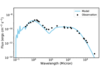
Figure 5: A comparison of the photometry data that comprises TW Hya’s SED and the modeled SED from RADMC3D based off of the gaseous and dust density and temperature structures from RAC2D.

3.4 Parameter Exploration

This study relies on a suite of CO line observations, as each line provides information about a slightly different vertical layer within the disk (Gorti et al., 2011; Zhang et al., 2017; Woitke et al., 2019). As the CO observations were spatially resolved, the quality of model was assessed by a comparison of the radial integrated intensity profiles. We additionally seek to match the HD flux and the SED.

As a first step we set up a grid of models to explore the full parameter space. The parameter space and initial model parameters from Zhang et al. (2019) are shown in Table 3. Initially, we explored gas mass, small dust mass, $\Psi$, $\gamma$, and radii and height values within ranges supported by previous observation and modeling work. Each parameter is explored using values above and below the initial value. For the gas mass, our upper limit was 0.06 $\textrm{M}_{\odot}$ which is the upper limit quoted in Bergin et al. (2013) and the lower limit was 0.01 $\textrm{M}_{\odot}$, which is similar to some earlier estimates of TW Hya’s gas mass (Weintraub et al., 1989b; Thi et al., 2010). The small dust mass range was motivated by the SED, limiting the range from factors of 2$\times$ greater than our initial value to $\sim$3$\times$ less. Both extremes produce SEDs that do not match the observations, but values in between provide a reasonable match to the SED. The $\Psi$ values explored vary from 0.8 to 1.3; both extremes affect the integrated CO emission profiles quite strongly. $\gamma$ has an upper limit of 2 (see Equation 1), however, we explore smaller variations on gamma around an initial value of 0.85, thus using limits of 0.5 - 1.1. We did not explore values nearing the upper limit of two as past observational constraints on $\gamma$ suggest the value for TW Hya is not much larger than 1.0 (Kama et al., 2016a; van Boekel et al., 2017; Zhang et al., 2017). While this is a narrow range, it did provide enough information to understand the trends that come from changes in $\gamma$. For $r_{exp_{\rm out}}$, $h_{c}$, and $r_{c}$, the smallest value explored was that of the large dust value, and the largest value explored was double the initial model value. We did not explore the inner nor outer edge values of $r_{s}$ (see Section 3.1) nor the inner exponential radial cutoff $r_{\rm exp_{\rm in}}$ as these values cannot be constrained with our CO observations. For each model we compare the model output CO isotopologue emission profiles as shown in Figure 4 in search of the best fit.

4 Results

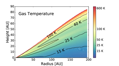
Figure 6: The final 2D thermal structure of the gas that reproduces seven resolved ALMA CO lines, HD flux, and the SED. The final temperature profile is supported up to scale heights from which ${}^{12}\textrm{CO}$ 2-1 emits from, since this transition has the highest optical depth

4.1 Description of Best-Fit Model

We show the results of our best-fit model in Figure 4, 5, and 6. The model agrees well with all seven resolved CO lines available along with the HD J=1-0 flux, and the SED profile (Figure 5). The parameter values of the best-fit model are given in Table 4.

Our beginning thermal structure was from the TW Hydra disk model of Zhang et al. (2019) (see Section 3.3). This initial model under-represents the CO flux in the inner $\sim$25 AU while over-representing the CO flux between 25 and 75 AU particularly in the ${}^{13}\textrm{CO}$ J=3-2 and $\textrm{C}^{18}\textrm{O}$ J=2-1 lines (see Figure 13). The initial model HD line flux is $4.6\times 10^{-18}$ $\textrm{W m}^{-2}$, which is 73% of the observed value, falling outside of the quoted error of that flux measurement from Bergin et al. (2013) $6.3(\pm 0.7)\times 10^{-18}$ $\textrm{W m}^{-2}$. To solve these initial discrepancies, we explore the parameter space extensively (see more details in the Appendix). We find that in order to match both CO and HD observations the $\Psi$ values of the gas and small dust need to be slightly different (1.1 and 1.2, respectively). This difference creates a thin layer at the surface of the disk which is depleted of dust. The difference between the scale height of the gas and dust is  1.2% of the radial location (represented in Figure 2).

This thin layer depleted of dust is a crude way to represent the impact of coagulation and settling on the small dust population end of the assumed MRN (Dullemond & Dominik, 2004). The changing values of $\Psi$ and thus scale heights can be seen as a way of representing a modified MRN distribution. Although the grain size distribution is not directly explored in this study, we find that the distribution of small grains strongly influences the final thermal structure. This relative change in scale height between dust and gas appears to be the best method to significantly increase the intensity of the CO emission in the inner 25 AU. Gas in this thin upper layer is more effectively heated as UV radiation penetrates more easily when the dust component is reduced. This heats CO gas in slightly denser regions and increases the CO emissivity.

Summing all these effects together, our best-fit model has a total gas mass that is only half of that in Zhang et al. (2019) model. This model predicts an HD flux of $5.9\times 10^{-18}$ $\textrm{W m}^{-2}$, which is well within the uncertainty of the observed flux.

4.2 Best-fit SED

The simulated SED as derived by our final TW Hya model was calculated using RADMC3D (Dullemond et al., 2012). After the temperature and physical distribution of the gas and dust were determined by RAC2D, we feed in those results including the stellar spectrum and dust opacities into RADMC3D.

Our model assumes a mass of small dust grains equal to $10^{-4}$ $\textrm{M}_{\odot}$ and a mass of the large dust grains to be $4\times 10^{-4}$ $\textrm{M}_{\odot}$. Using these dust components, our model SED agrees reasonably well with the observed SED, see Figure 5. TW Hydra also exhibits a strong silicate feature near 10 µm which our dust model under predicts. Previous studies that have successfully modeled this feature by utilizing a special type of silicate within 4 AU (Calvet et al., 2002; Zhang et al., 2013). This is a scale much smaller than we aim to constrain, and is a small effect in comparison to the total dust opacity in this region. The SED beyond $\sim$8 µm tests if we are correctly representing the dust population, as the long-wavelength portion of the SED is mostly affected by dust mass, size distribution, spatial distribution, and composition (a mixture of silicates and graphite). Overall, our dust model provides a good match to the observed SED. Since the small dust population has an effect on the thermal balance, the SED provides one of the key factors to constrain the HD emission and overall disk mass.

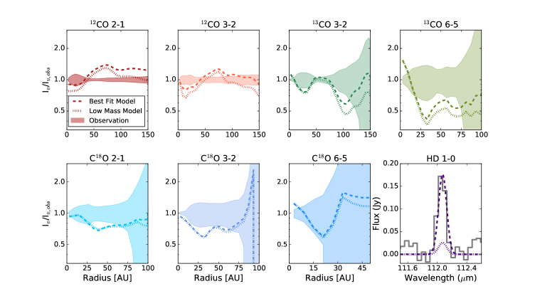
Figure 7: The radial intensity profiles of the observations, best fit model, and low mass model all normalized to the observations, along with the HD flux observations compared to the simulated HD flux in the low mass model. The observations are thus located at 1, and are the solid line while the models are dashed lines with the thick dashed line representing the best fit model (see Figure 4) and the low mass model (with high CO abundance) represented with the thinner dashed line. Errors of the integrated intensity line profile is shown in the shaded region, and is also normalized by the observed intensity. From this comparison, we can see that both the model with a gas mass of 0.023 $\textrm{M}_{\odot}$ and 0.0023 $\textrm{M}_{\odot}$ have nearly identical profiles. This also shows how close our model represents the observations. The majority of the time, the modeled flux is within a factor of two of the observed, with the only exceptions being when the observations drop quickly to receive zero flux and the model does not reach zero as quickly, however the model still is within the error. This happens especially with $\textrm{C}^{18}\textrm{O}$ 6-5. While in the low mass model, the CO remains relatively similar, the HD flux drops significantly.

4.3 ${}^{13}C^{18}O$ Flux

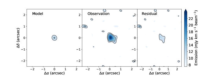
Figure 26: ALMA observation of ¹³C¹⁸O $J$=3-2 line emission (middle panel) as compared to our final TW Hya modeled ¹³C¹⁸O $J$=3-2 flux (left panel), and the residual (right panel). Contours are trace the location of 9 and 13 mJy flux values.

Using our final model, we seek to compare the observed ¹³C¹⁸O flux towards TW Hya as presented in Zhang et al. (2017). We use line information for ¹³C¹⁸O derived by HITRAN (Rothman et al., 2005), formatted to be identical to line data from the Leiden Atomic and Molecular Database. We also use an abundance ratio ${}^{12}\textrm{CO}$/${}^{13}\textrm{CO}$ = 40, as measured by Zhang et al. (2017) for this specific observation. The resultant flux is shown in Appendix Figure 26. Overall, our model provides a good fit to the observations, underpredicting the ¹³C¹⁸O flux by at most by 12 mJy km s^-1 beam^-1, or about a factor of two across the modeled flux emitting area. As the ¹³C¹⁸O emission is highly centrally concentrated the location of largest discrepancy is in the central regions and also towards the observed asymmetry. This residual value is similar to the background noise flux. The asymmetry can be accounted for by simply the low signal/noise ratio for this observation.

4.4 CO Mass/Abundance Degeneracy

Our exploration of the parameter space shows that the CO line intensity is a degenerate result of the total gas mass and CO abundance. If the line is optically thin, the CO emission scales directly with its number density, $n_{\ce{CO}}$, where $n_{\ce{CO}}$ is $x_{\rm CO}\times$ $n_{\rm H_{2}}$. Even in the case of optically thick lines, as the gas density increases, CO emission becomes optically thick at a higher location of the disk atmosphere; thereby tracing temperature of a warmer region. Thus there is a degeneracy between the abundance of CO and the density of $\textrm{H}_{2}$ and hence the gas mass. One way to break this degeneracy is with an observed HD flux, as it is independent of CO abundance.

To explore this, we create a low-mass model based on the parameters of our best-fit model, however in this model we decrease the total gas mass by one order of magnitude while subsequently increasing in the CO abundance by the same factor. As shown in Fig. 7 this low mass model produces indistinguishable CO radial profiles compared to these of our best-fit model. However, the line flux of HD (1-0) transition of the lower mass model goes down by more than a factor of five (see bottom right panel in Figure 7). This degeneracy between CO abundance and gas mass has been reported in previous studies with less well-constrained temperature structures. (Bergin et al., 2013; Favre et al., 2013; McClure et al., 2016; Kama et al., 2016a; Trapman et al., 2017). Here we prove that the degeneracy cannot be broken even the thermal structure of the disk is well constrained. In short, CO lines alone are not sufficient to constrain the total disk mass and another independent mass tracer must be introduced, such as HD.

5 Analysis & Discussion

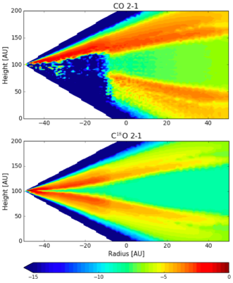
Figure 8: The emitting regions of ${}^{12}\textrm{CO}$ and $\textrm{C}^{18}\textrm{O}$ 2-1 in our final model. Emitting regions for each molecule were calculated based on the final model, and were used to create Figure 9, which encapsulates the regions in which most of each molecule is emitting from.

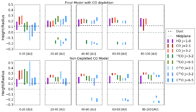
Figure 9: The average vertical emitting region of each line used in this study for our final model (top) and a version of that model without assuming CO depletion (bottom). For every 20 AU the average vertical emitting height was calculated. The top of each bar corresponds to the average surface which consists of 90% of the flux. The bottom of the bar and below is 10% of the total flux. Lines that have two emitting regions, one above the disk and below, are optically thin, thus observations of these molecules come from both the front and back of the disk. There is no emission in the midplane outside the CO snowline, thus for an optically thin emitter, their emitting regions were calculated twice. Once for above the midplane, then again but only from the back. The continuous $\tau=1$ surface of the dust at the frequency of HD J=1-0 is shown via the dashed line. Examples of 2D contribution plots used to create this figure of ${}^{12}\textrm{CO}$ 2-1 and $\textrm{C}^{18}\textrm{O}$ 2-1 are shown in Figure 8.

5.1 CO Emitting Regions

RAC2D calculates the emitting regions for each isotopologue; examples of ${}^{12}\textrm{CO}$ 2-1 and $\textrm{C}^{18}\textrm{O}$ 2-1 are shown in Figure 8. To allow for inter-molecular comparison, we then calculated the heights at which the majority of the emission originates. This is presented in Figure 9 where we show a visualization of the average vertical cross-section of the disk from which each line is emitting based on our final model. For comparison, a non-CO depleted model is also shown. A dashed line representing the $\tau=1$ surface of the small dust at the frequency of the HD $J$=1-0 transition ($\lambda\simeq 112\micron$) is plotted as a reference. These two models represent two extremes of T Tauri disks, a high CO abundance (which corresponds to a CO/$\textrm{H}_{2}$ ratio equal to that of the ISM) and a low CO abundance, using the relatively high CO depletion factors found in TW Hya.

In the non-depleted case, ${}^{12}\textrm{CO}$ emits from a higher layer than all other isotopologues, while HD and ${}^{13}\textrm{CO}$ and in some cases $\textrm{C}^{18}\textrm{O}$, probe similar depths. $\textrm{C}^{18}\textrm{O}$ appears to be optically thin, especially past 60 AU; the $\textrm{C}^{18}\textrm{O}$ surface brightness is therefore not a sufficient temperature tracer across a disk with similar properties as TW Hya. In this instance $\textrm{C}^{18}\textrm{O}$ probes the total column density. TW Hya is, however, is thought to exhibit severe CO depletions, thus CO and its isotopologues emission will have reduced optical depth (in comparison to the non-depleted model). In our final model, ${}^{12}\textrm{CO}$ 2-1, 3-2, and ${}^{13}\textrm{CO}$ 3-2 emit from roughly an equivalent vertical depth as HD, showing that in this disk, observations of ${}^{12}\textrm{CO}$ 2-1, 3-2 and ${}^{13}\textrm{CO}$ 3-2 best trace the layers where HD emission arises. Within radii ranging from 0 - 40 AU, ${}^{13}\textrm{CO}$ 3-2 emission is optically thick, overlapping with the lower bound of the HD emitting layer. The $\textrm{C}^{18}\textrm{O}$ and ${}^{13}\textrm{CO}$ 6-5 become optically thin beyond radii of 20-40AU, thus their brightness temperature no longer constrains the disk surface temperature. Based on this result, the disk mass for TW Hya could have been accomplished using only the resolved observations of ${}^{12}\textrm{CO}$ 2-1, 3-2, and supplemented with ${}^{13}\textrm{CO}$ 3-2 alongside HD. For future observations, multiple observations of CO are still required, at least down to the 3-2 levels, as CO depletion and gas mass are not known a priori.

5.2 Scattered Light Effects

TW Hya has been observed in scattered light, which traces out the small dust population of the disk. These observations are reported in van Boekel et al. (2017), and using the scattered light observations they find that radial depressions in the small dust surface density are necessary to reproduce the observed surface brightness. The two largest depressions in the surface density have depths 80% and 45% at approximately 5 AU and 90 AU, respectively (see Figure 11 in van Boekel et al., 2017). We applied this depletion factor to the small dust population to the initial model and found that it did not strongly effect the radial profiles as shown in Figure 10. The depletion does increase the HD $J$ = 1-0 flux by 30%. However, the effect on ¹²CO and C¹⁸O is much less (below 15%), and these changes do not significantly alter the fit to the CO radial profiles. Future modeling efforts may want to include information from the mm-continuum and scattered light observations as an additional constraint on the physical state of surface layers.

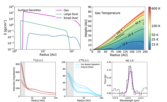
Figure 10: At the upper left are the surface densities for the gas and dust populations while taking a depletion of small dust as measured by van Boekel et al. (2017) from scattered light observations. Using the new small dust population, we calculate the gas temperature (top right), the radial profiles of ${}^{12}\textrm{CO}$ and $\textrm{C}^{18}\textrm{O}$ 2-1 (bottom middle, left), and HD flux. The dashed lines in the radial profile and HD flux plot show our initial model, compared to a model with a non-smooth small dust surface density as motivated by the scattered light observations.

5.3 Comparison to Other Models

There are at least two other attempts to model TW Hydra with thermo-chemical codes: Kama et al. (2016b) with the DALI 2D physical-chemical code, and Woitke et al. (2019) with the ProDiMo code.

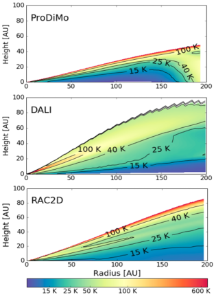
Figure 11: A comparison of the gas thermal structure of TW Hya from Woitke et al. (2019), Kama et al. (2016b), and this study.

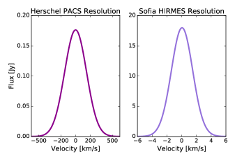
Figure 12: A predicted HD spectra based on the resolution of the proposed HIRMES instrument on Sofia (right) compared to the modeled spectra of HD J=1-0 from this study using the spectral resolution of the PACS instrument.

Kama et al. (2016b) focused on tracing volatile carbon in TW Hya. To do so, they modeled an underlying thermal structure of both the gas and dust population using DALI (Bruderer et al., 2009, 2012; Bruderer, 2013) which is designed and operated in a very similar way to RAC2D. This study utilized spatially unresolved observations of the CO ladder (upper limits of $J$=36-35, 33-32, 29-28, and line fluxes of $J$=18-17, 10-9, 6-5, ALMA observation of $J$=3-2, and SMA observation of $J$=2-1). Their observation of CO $J$ 3-2 was spatially resolved. Additionally, they utilized other carbon carrier molecules (C[I], C[II], $\textrm{C}_{2}\textrm{H}$, $\textrm{HCO}^{+}$) to motivate their models along with HD both J=1-0 and J=2-1. Kama et al. (2016b) produced a model that reproduces their CO observations and the HD flux. DALI has since been updated to include deuterium chemistry and isotoplogue selective chemistry following work by Miotello et al. (2014). This subsequent updated model is presented in Trapman et al. (2017) and shown in Figure 11, alongside our RAC2D results. The main difference between Kama et al. (2016a) model and ours is that we reproduce multiple spatially resolved CO transitions. Our $\sim$15 - 100 K isotherms match up relatively well, which are the temperature ranges that our CO lines trace. Our solutions do diverge from each other at high temperatures ($>100$K). Using the HD emission, Kama et al. (2016b) derived gas mass, and determined the same value that this study independently arrived at: 0.023 $\textrm{M}_{\odot}$.

Woitke et al. (2019) describes the DIANA project, which modeled a number of protoplanetary disks in a homogeneous way using SED-matching and the thermo-chemical code ProDiMo. Their model outputs for each disk are publicly available. Figure 11 shows a comparison of their results with our RAC2D model. The most noticeable difference is that our model appears to have a higher gas scale height compared to that determined by the DIANA project. Further, the DIANA model finds higher gas temperatures at the disk surface, along with a comparatively cooler midplane (e.g. compare 15 K isotherms). Woitke et al. (2019) matched many volatile lines such as CO and $\textrm{H}_{2}\textrm{O}$ to within a factor of two. However they under predicted the HD emission by a factor of 13 with a total gas mass of 0.045 $\textrm{M}_{\odot}$.

Cleeves et al. (2015) also produced a TW Hya model with the primary goal of fitting molecular ion observations. In the process, this paper used SMA observations of $\textrm{C}^{18}\textrm{O}$ and ${}^{13}\textrm{CO}$ J=2-1 and the Herschel HD observation to constrain the physical structure. The chemical model employed was not a self consistent thermo-chemical model, however, the gas temperature structure was derived via a DALI-based fitting function to account for the gas and dust thermal decoupling in the upper layers. In the Cleeves et al. (2015) model, the derived gas mass of 0.04$\pm$0.02 M_⊙ is also in good agreement with our best fit model, as is the overall temperature profile.

5.4 Future Observations of Spatially Resolved CO Line Emission in Inclined Disks

This study serves as a proof of concept that observation and subsequent modeling of resolved CO lines and HD line flux in combination with the SED is a powerful method to uncover thermal structure and disk mass. TW Hya is an ideal disk to test out this new method, as it is has been extensively observed with ALMA and other observatories, and is one of only three disks with an HD emission detection (McClure et al., 2016). One disk parameter not explored in this particular study is disk inclination. An inclined disk will allow for direct constraints to be set on the vertical emitting layer and the subsequent temperature inferred within the layer (Pinte et al., 2018; Teague et al., 2019). Disk inclination will broaden the spectral line, and the degree at which that might complicate extraction of a 2D thermal structure using thermo-chemical models is worth investigation. It is also worth applying these techniques towards brighter Herbig Ae/Be disks. The CO snowline in these systems lies at greater distances from the star (Qi et al., 2015; Zhang et al., 2020a) and hence some transitions might probe layers closer to the midplane than sampled in T Tauri systems.

In our model we do not take CO fractionation chemistry into account. However, this would not effect the derived temperature structure very strongly. ${}^{12}\textrm{CO}$ would be unaffected and selective photodissociation has a marginal effect for ${}^{13}\textrm{CO}$. There would be a larger effect for $\textrm{C}^{18}\textrm{O}$; however its emission is optically thin for much of the disk and thus does not provide sufficient temperature information. We also did not include rarer isotopologues of CO such as ¹³C¹⁸O (Zhang et al., 2017), which would provide additional insight into column density inside the CO snowline.

5.5 Future HD observations

At present, the sample of disks in which HD has been targeted is limited to a few deep observations (McClure et al., 2016) and those with full Herschel PACS scans, such as the upper limits on HD emission in Herbig disks by Kama et al. (2019). More observations are necessary to further our understanding of protoplanetary disks. There are future instruments and observatories potentially on the horizon that will observe the frequency range in which HD resides, and with a much higher resolution and sensitivity than Herschel. These observatories will have the ability to drastically improve our understanding of early planet formation environments. The HIRMES instrument was proposed to be added to the SOFIA observatory offering a spectral resolution of 3 km s^-1 at 112 $\micron$. If built and deployed, HIRMES was projected to have a sensitivity similar to PACS (Richards et al., 2018) and could perform deep surveys for HD emission, opening up the ability to provide a robust diagnostic of gas mass. The planned spectral resolution on HIRMES is enough to fully resolve the HD emission line for inclined disks, which will provide unique constraints on the radial distribution of disk gas. A simulated HIRMES observation of TW Hya based on this model is shown in Figure 12.

Looking onward, National Aeronautics and Space Administration’s (NASA) Origins Space Telescope, if funded and launched, provides a sensitivity improvement at 112 µm of over three orders of magnitude compared to Herschel, enabling deep surveys of over a thousand disks. Origins could provide sensitivities towards the HD line corresponding to gas disk masses down to $10^{-5}$ $\textrm{M}_{\odot}$(Trapman et al., 2017). These future or potential observatories in combination with future resolved suites of CO lines via ALMA will be incredibly insightful towards out understanding of planet formation enabling the ability to track the 2D temperature structure and the gas mass, thereby revealing the key physical conditions under which planets form.

6 Conclusions

Using the thermo-chemical code RAC2D, and observations from the TW Hya Rosetta Project taken with ALMA of ${}^{12}\textrm{CO}$ $J$= 2-1, $\textrm{C}^{18}\textrm{O}$ $J$= 2-1, archival ALMA data of ${}^{12}\textrm{CO}$ 3-2, $\textrm{C}^{18}\textrm{O}$ 3-2, 6-5, and ${}^{13}\textrm{CO}$ 3-2, 6-5, HD $J$ 1-0, and the system’s SED, we find the following:

1. We derive a thermal structure of the TW Hya disk that fits radial brightness profiles of seven spatially resolved CO line transitions, a spatially unresolved HD line flux, and the SED. This study is the first to reproduce multiple spatially resolved observations of CO using a thermo-chemical model. We compare our results to thermal structures derived by other methods.

2. Using the derived thermal structure and the HD (1-0) line flux, we constrain the total gas mass of the TW Hya disk to be $\approx$ 0.025 $\textrm{M}_{\odot}$ within our model framework.

3. We directly demonstrate that CO line brightness distributions are degenerate results of the CO abundance and the total gas mass of the disk. Therefore CO alone cannot be used as a robust tracer of the total gas mass, for any protoplanetary disk system. We find that using observations of HD is one solution that breaks this degeneracy.

7 Acknowledgments

This paper makes use of data from ALMA programs 2015.1.00686.S, 2016.1.00629.S, 2012.1.00422.s, and 2016.1.00311.S. ALMA is a partnership of ESO (representing its member states), NSF (USA) and NINS (Japan), together with NRC (Canada) and NSC and ASIAA (Taiwan), in cooperation with the Republic of Chile. The Joint ALMA Observatory is operated by ESO, AUI/NRAO and NAOJ. The National Radio Astronomy Observatory is a facility of the National Science Foundation operated under cooperative agreement by Associated Universities, Inc. J.K.C. acknowledges support from the National Science Foundation Graduate Research Fellowship under Grant No. DGE 1256260 and the National Aeronautics and Space Administration FINESST grant, under Grant no. 80NSSC19K1534. E.A.B. acknowledges support from NSF grant No. 1907653. K.S. acknowledges the support of NASA through Hubble Fellowship grant HST -HF2-51401.001 awarded by the Space Telescope Science Institute, which is operated by the Association of Universities for Research in Astronomy, Inc., for NASA, under contract NAS5-26555. L.I.C. gratefully acknowledges support from David and Lucile Packard Foundation and the Virginia Space Grant Consortium. J. H. acknowledges support from the National Science Foundation Graduate Research Fellowship under Grant No. DGE-1144152. S. A. and from the National Aeronautics and Space Administration under Grant No. 17-XRP17 2-0012 issued through the Exoplanets Research Program. Support for this work was provided by NASA through the NASA Hubble Fellowship grant #HST-HF2-51460.001-A awarded by the Space Telescope Science Institute, which is operated by the Association of Universities for Research in Astronomy, Inc., for NASA, under contract NAS5-26555. C.W. acknowledges financial support from the University of Leeds and the Science and Technology Facilities Council (STFC; grant No. ST/R000549/1). M.K. gratefully acknowledges funding by the University of Tartu ASTRA project 2014-2020.4.01.16-0029 KOMEET “Benefits for Estonian Society from Space Research and Application”, financed by the EU European Regional Development Fund

Appendix A Parameter Effects on Simulated Observations

Through exploration of our model and the parameter space of the properties listed in Table 3, we find that CO emission is most strongly affected by gas and small dust parameters. Here we list how the CO integrated intensity profiles respond to changes in parameters. These findings are specific to this TW Hya model, but can be extrapolated to similarly inclined gaseous disks. The following discussion is based off of the model parameter values from Zhang et al. (2019) presented in Figure 13:

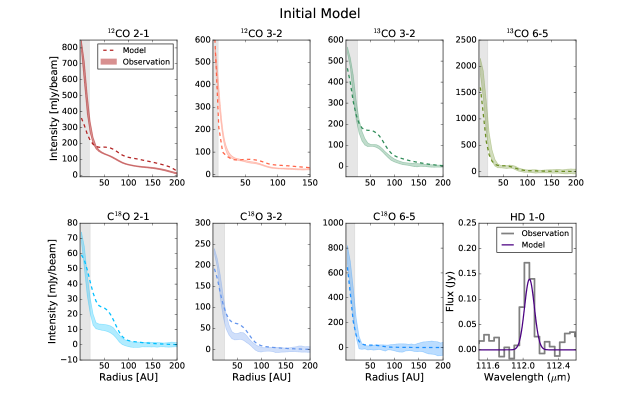
Figure 13: The integrated line profiles of CO and its isotopologues from ALMA observations (solid lines) and the simulated observations from RAC2D using model parameters from Zhang et al. (2019), and listed in Table 3

A.1 $\gamma$ : Power-law Index of Surface Density

$\gamma$ is a power-law index for the surface density (see Equation 1) with a maximum value of two. Increasing $\gamma$ affects the distribution by concentrating the given component (gas, dust) towards the inner disk region, increasing the column density of gas and dust. A decrease in $\gamma$ results in a more even distribution of the mass component. It has the strongest effect on the emission arising from the inner 25 AU, especially for the rare isotopologues. Altering gamma from 0.75 to 0.9 in both small dust and gas results in very little change in ${}^{12}\textrm{CO}$ 2-1 and 3-2, but at least a 10% increase across all $\textrm{C}^{18}\textrm{O}$ lines. In our final model, we increased $\gamma$ in both the gas and small dust, as they are coupled, from 0.75 to 0.85 which aided in adding to the intensity in the inner 25 AU.

Figure 14: The integrated intensity profiles of observations and a model based of the initial model (13) but with $\gamma$ in the gas and small dust = 0.5.

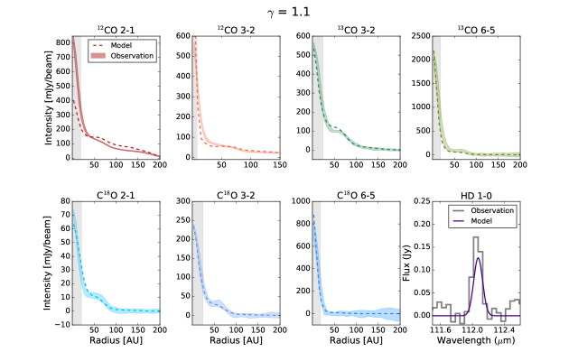
Figure 15: The integrated intensity profiles of observations and a model based of the initial model (13) but with $\gamma$ in the gas and small dust = 1.1.

A.2 $\Psi$ : Power-law Index For Scale Height

Typical $\Psi$ values are between 1.1 and 1.2 for TW Hya, and affects the scale height over different radii, with an increase in the flaring as $\Psi$ increases. Changes in $\Psi$ down to 0.05 have a significant effect on the final integrated intensity profiles. Generally, lowering $\Psi$ results in an increase in intensity in the inner disk ($<$ 25 AU), and beyond $\approx$ 25 AU features are ‘smoothed’ ouft. This is due to the increase of gas surface density towards the inner AU when flaring decreases. The most extreme value of $\Psi$ we explored was 1.6, and at that point the modeled intensity profiles plummeted down to between 25% of their original flux to zero within 20 AU. Beyond 20 AU, there is emission comparable to the original model. The thermal profile derived from the initial parameters (shown in Table 3 and discussed in Section 3.3) produced CO lines that were too dim within 25 AU by a factor of 2 in ${}^{12}\textrm{CO}$, ${}^{13}\textrm{CO}$ 6-5, $\textrm{C}^{18}\textrm{O}$ 6-5 and $\sim$ 30% in ${}^{13}\textrm{CO}$ and $\textrm{C}^{18}\textrm{O}$ 3-2. We find that the only way to significantly brighten the inner regions while simultaneously keeping the intensity in the outer regions low is to allow the gas and small dust to have slightly different $\Psi$ values. The gas component is given a $\Psi$ value of 1.1, while the small dust is given $\Psi$= 1.2. Due to the fact that our critical radius is beyond the gaseous radius, even though the dust has a higher flaring angle, it lies below the gas. This creates a thin region at the upper layer of the disk where only gas resides; this region has a thickness of $\sim$ 1.2% of a given radius. In this gas-rich layer, CO and HD lines become brighter, noticeably within the inner few AU. There are no other parameters that we explored that accomplished this, the closest being $\gamma$, which increases emission within 50 AU, but smooths out the feature beyond 50 AU.

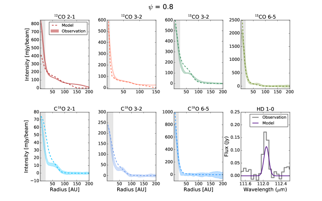
Figure 16: The integrated intensity profiles of observations and a model based of the initial model (13) but with $\Psi$ in the gas and small dust = 0.4.

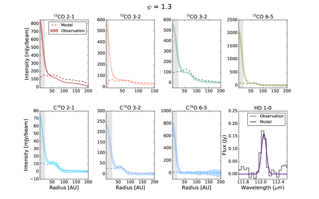
Figure 17: The integrated intensity profiles of observations and a model based of the initial model (13) but with $\Psi$ in the gas and small dust = 1.6.

A.3 Gas Mass

An increase in the total gas mass increases the intensity from each line along all radii. A higher gas mass results in a higher column density for each molecule, and some of the CO lines (especially ${}^{12}\textrm{CO}$ 2-1) are already optically thick in explored mass range. There are also isotopologues whose emission is not fully optically thick in the lower mass models, thus changes in their column have a strong effect on their flux. Increasing the gas mass from 0.01 to 0.02 $\textrm{M}_{\odot}$ doubles the peak integrated flux in $\textrm{C}^{18}\textrm{O}$, a 25% increase in ${}^{13}\textrm{CO}$, and ${}^{12}\textrm{CO}$ 3-2 and an increase of $\sim$ 20% in ${}^{12}\textrm{CO}$ 2-1. Our best-fit model has a disk mass of 0.023 solar masses. We arrived at this value only after the gas and small dust components of our model were given different $\Psi$ values. With a gas mass of 0.05 $\textrm{M}_{\odot}$ and $\Psi_{\rm gas}$ = 1.1 and $\Psi_{\textrm{small dust}}$ = 1.2, the HD flux increases by a factor of two, and emission in CO at large radii also increases by a factor of 2-3 depending on the isotopologue. Due to this, a decrease in total gas mass is justified. Decreasing the mass to 0.023 $\textrm{M}_{\odot}$ brings the HD flux back down to what Herschel observed, and brings the CO emission back down to values that agree with ALMA observations.

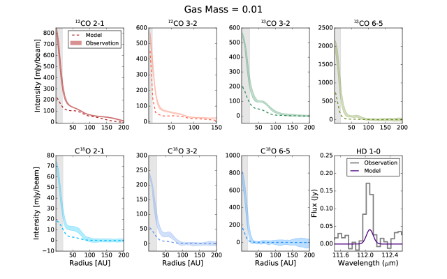
Figure 18: The integrated intensity profiles of observations and a model based of the initial model (13) but with a gas mass equal to 0.01 $\textrm{M}_{\odot}$

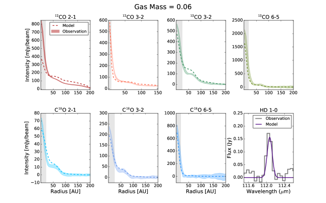
Figure 19: The integrated intensity profiles of observations and a model based of the initial model (13) but with a gas mass equal to 0.06 $\textrm{M}_{\odot}$

A.4 Small Dust Component Mass

Given a constant gas mass of 0.05 $\textrm{M}_{\odot}$ and a starting small dust mass of 1.0 $\times 10^{-4}$ $\textrm{M}_{\odot}$ or higher, decreasing the small dust mass has a similar effect as increasing gas mass. At 1.0 $\times 10^{-4}$ $\textrm{M}_{\odot}$ and lower, flux beyond 20 AU increases at a faster rate than within 20 AU, leading to exaggerated features, such as the plateaus in $\textrm{C}^{18}\textrm{O}$ 2-1 and 3-2 becoming peaks at small dust masses less than 2.5 $\times 10^{-5}$ $\textrm{M}_{\odot}$. The small dust population absorbs and scatters radiation and in some instances leads to a CO line profile that is extincted. Eliminating small dust allows for the gas that exists to emit more freely as a major opacity source is removed. The small dust mass is particularly impactful on the HD emission, because the small dust governs the propagation of UV radiation, with smaller dust masses allowing UV photons from the star to penetrate deeper layers of the disk, directly affecting the gas heating terms. This helps populate the HD $J$=1 level, increasing the HD $J$=1-0 line flux. In our final model, we were not strongly motivated to change the small dust mass beyond what had been initially predicted, but it could be a useful lever in future modeling of disks. At present the strongest constraint on the mass of the small dust is the SED and scattered light emission form the surface.

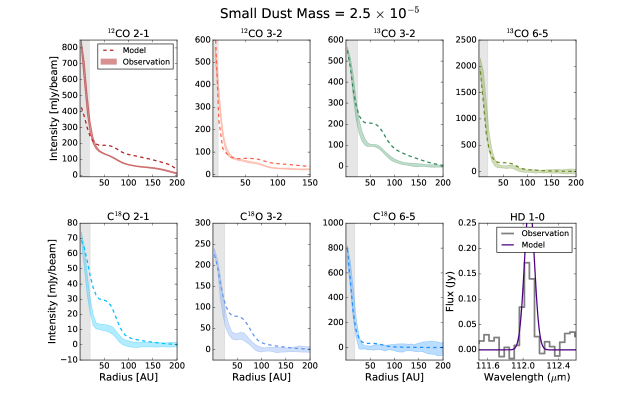
Figure 20: The integrated intensity profiles of observations and a model based of the initial model (13) but with a total small dust mass equal to 2.5 $\times$ 10^-5 $\textrm{M}_{\odot}$

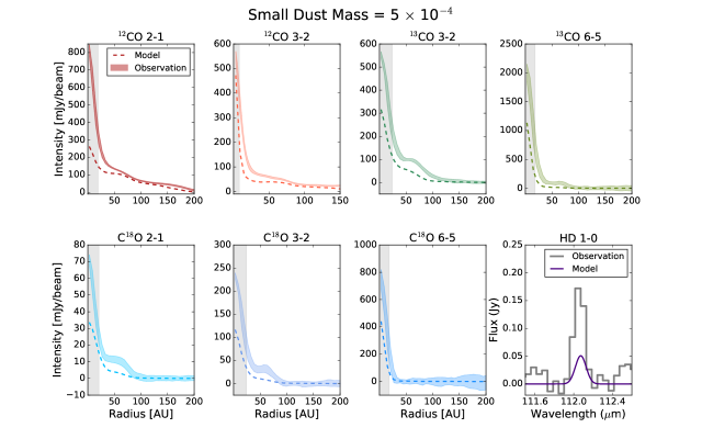
Figure 21: The integrated intensity profiles of observations and a model based of the initial model (13) but with a total small dust mass equal to 5 $\times$ 10^-4 $\textrm{M}_{\odot}$

A.5 $\rm r_{\textrm{exp}}$ : Outer Tapering Radius

At this specified radius the abundance of a component exponentially decreases. Altering the $r_{\textrm{exp}}$ effects outer disk emission, as it significantly depletes the corresponding component. It is only significant in ${}^{12}\textrm{CO}$ 2-1 and 3-2, as these are the only intensity profiles with emission beyond 100 AU. If the gas and small dust $r_{\textrm{exp}}$ value becomes less than the large dust $r_{\textrm{exp}}$, the effect is much stronger and acts similar to decreasing $\gamma$.

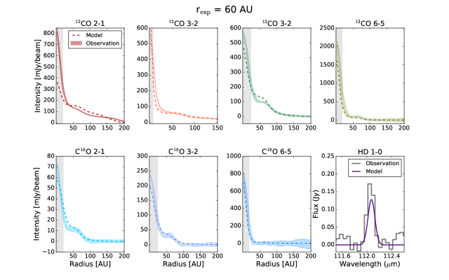
Figure 22: The integrated intensity profiles of observations and a model based of the initial model (13) but with r${}_{\rm exp_{\rm out}}$ in the gas and small dust = 60 AU

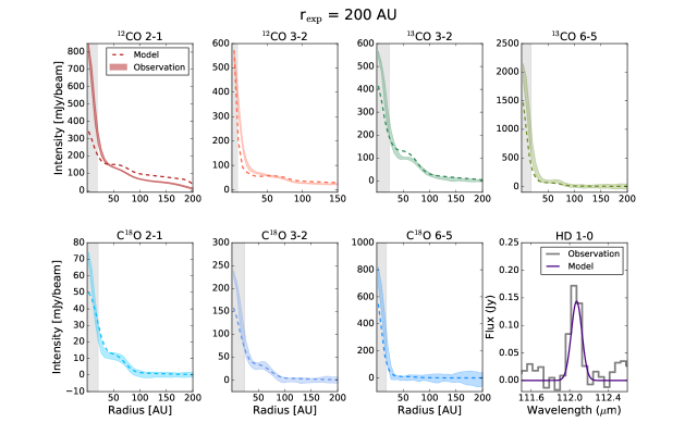
Figure 23: The integrated intensity profiles of observations and a model based of the initial model (13) but with r${}_{\rm exp_{\rm out}}$ in the gas and small dust = 200 AU

A.6 $\rm h_{c}$: Characteristic Height

An increase of the height of the disk results in an increase in intensity across all radii and in all molecules, with the ones most strongly affected being the least abundant. A change in scale height increases the column that one observes, which then increases the flux of an optically thin molecule. However, this does not strongly affect optically thick molecules. An increase of two times the scale height only results in a $\sim$ 5 % increase in peak intensity in ${}^{12}\textrm{CO}$ 2-1 and a full 20% increase in the least common isotopologue transition considered here, $\textrm{C}^{18}\textrm{O}$ 6-5.

The scale height, scale radius, $\Psi$, and $\gamma$ of the large dust population do not have strong effects on the CO line profiles. The temperature of the star also does not have a strong effect; a change in 1000 K resulted in only a  1% increase across all lines.

The parameters we find having the largest impact on the CO and HD flux were: gas mass, the flaring parameter $\Psi$, surface density distribution parameter $\gamma$, and small dust mass. The gas mass affects all CO lines, and has a stronger influence on the optically thin lines. $\Psi$ and $\gamma$ both redistribute flux between the inner and outer regions of the disk depending on where the majority of the gas component is located. The small dust mass was not a parameter that needed to be altered from its initial value, but has a strong effect on the HD flux and could be utilized in future studies as long as the SED is taken into account.

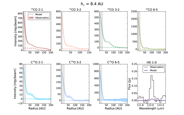
Figure 24: The integrated intensity profiles of observations and a model based of the initial model (13) but with h_c in the gas and small dust = 8.4 AU

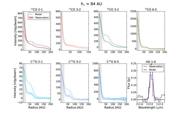
Figure 25: The integrated intensity profiles of observations and a model based of the initial model (13) but with h_c in the gas and small dust = 84 AU

References

- Aikawa et al. (2002) Aikawa, Y., van Zadelhoff, G. J., van Dishoeck, E. F., & Herbst, E. 2002, A&A, 386, 622, doi: 10.1051/0004-6361:20020037
- Andrews (2020) Andrews, S. M. 2020, arXiv e-prints, arXiv:2001.05007. https://arxiv.org/abs/2001.05007
- Andrews et al. (2010) Andrews, S. M., Czekala, I., Wilner, D. J., et al. 2010, ApJ, 710, 462, doi: 10.1088/0004-637X/710/1/462
- Andrews et al. (2012) Andrews, S. M., Wilner, D. J., Hughes, A. M., et al. 2012, ApJ, 744, 162, doi: 10.1088/0004-637X/744/2/162
- Ansdell et al. (2016) Ansdell, M., Williams, J. P., van der Marel, N., et al. 2016, ApJ, 828, 46, doi: 10.3847/0004-637X/828/1/46
- Bailer-Jones et al. (2018) Bailer-Jones, C. A. L., Rybizki, J., Fouesneau, M., Mantelet, G., & Andrae, R. 2018, AJ, 156, 58, doi: 10.3847/1538-3881/aacb21
- Bergin & Cleeves (2018) Bergin, E. A., & Cleeves, L. I. 2018, Chemistry During the Gas-Rich Stage of Planet Formation, 137, doi: 10.1007/978-3-319-55333-7_137
- Bergin & Williams (2017) Bergin, E. A., & Williams, J. P. 2017, Astrophysics and Space Science Library, Vol. 445, The Determination of Protoplanetary Disk Masses, ed. M. Pessah & O. Gressel, 1, doi: 10.1007/978-3-319-60609-5_1
- Bergin et al. (2013) Bergin, E. A., Cleeves, L. I., Gorti, U., et al. 2013, Nature, 493, 644, doi: 10.1038/nature11805
- Birnstiel et al. (2012) Birnstiel, T., Klahr, H., & Ercolano, B. 2012, A&A, 539, A148, doi: 10.1051/0004-6361/201118136
- Bisschop et al. (2006) Bisschop, S. E., Fraser, H. J., Öberg, K. I., van Dishoeck, E. F., & Schlemmer, S. 2006, A&A, 449, 1297, doi: 10.1051/0004-6361:20054051
- Bosman et al. (2018) Bosman, A. D., Walsh, C., & van Dishoeck, E. F. 2018, A&A, 618, A182, doi: 10.1051/0004-6361/201833497
- Brickhouse et al. (2010) Brickhouse, N. S., Cranmer, S. R., Dupree, A. K., Luna, G. J. M., & Wolk, S. 2010, ApJ, 710, 1835, doi: 10.1088/0004-637X/710/2/1835
- Bruderer (2013) Bruderer, S. 2013, A&A, 559, A46, doi: 10.1051/0004-6361/201321171
- Bruderer et al. (2009) Bruderer, S., Doty, S. D., & Benz, A. O. 2009, ApJS, 183, 179, doi: 10.1088/0067-0049/183/2/179
- Bruderer et al. (2012) Bruderer, S., van Dishoeck, E. F., Doty, S. D., & Herczeg, G. J. 2012, A&A, 541, A91, doi: 10.1051/0004-6361/201118218
- Calvet et al. (2002) Calvet, N., D’Alessio, P., Hartmann, L., et al. 2002, ApJ, 568, 1008, doi: 10.1086/339061
- Cleeves et al. (2015) Cleeves, L. I., Bergin, E. A., Qi, C., Adams, F. C., & Öberg, K. I. 2015, The Astrophysical Journal, 799, 204, doi: 10.1088/0004-637X/799/2/204
- Cleeves et al. (2018) Cleeves, L. I., Öberg, K. I., Wilner, D. J., et al. 2018, ApJ, 865, 155, doi: 10.3847/1538-4357/aade96
- Cutri et al. (2003) Cutri, R. M., Skrutskie, M. F., van Dyk, S., et al. 2003, 2MASS All Sky Catalog of point sources.
- Debes et al. (2013) Debes, J. H., Jang-Condell, H., Weinberger, A. J., Roberge, A., & Schneider, G. 2013, ApJ, 771, 45, doi: 10.1088/0004-637X/771/1/45
- Du & Bergin (2014) Du, F., & Bergin, E. A. 2014, ApJ, 792, 2, doi: 10.1088/0004-637X/792/1/2
- Dullemond & Dominik (2004) Dullemond, C. P., & Dominik, C. 2004, A&A, 421, 1075, doi: 10.1051/0004-6361:20040284
- Dullemond et al. (2012) Dullemond, C. P., Juhasz, A., Pohl, A., et al. 2012, RADMC-3D: A multi-purpose radiative transfer tool. http://ascl.net/1202.015
- Eistrup et al. (2018) Eistrup, C., Walsh, C., & van Dishoeck, E. F. 2018, A&A, 613, A14, doi: 10.1051/0004-6361/201731302
- Favre et al. (2013) Favre, C., Cleeves, L. I., Bergin, E. A., Qi, C., & Blake, G. A. 2013, The Astrophysical Journal, 776, L38, doi: 10.1088/2041-8205/776/2/L38
- Fayolle et al. (2016) Fayolle, E. C., Balfe, J., Loomis, R., et al. 2016, ApJ, 816, L28, doi: 10.3847/2041-8205/816/2/L28
- Fedele et al. (2016) Fedele, D., van Dishoeck, E. F., Kama, M., Bruderer, S., & Hogerheijde, M. R. 2016, A&A, 591, A95, doi: 10.1051/0004-6361/201526948
- Fraser et al. (2001) Fraser, H. J., Collings, M. P., McCoustra, M. R. S., & Williams, D. A. 2001, MNRAS, 327, 1165, doi: 10.1046/j.1365-8711.2001.04835.x
- Frerking et al. (1982) Frerking, M. A., Langer, W. D., & Wilson, R. W. 1982, ApJ, 262, 590, doi: 10.1086/160451
- Gaia Collaboration et al. (2018) Gaia Collaboration, Brown, A. G. A., Vallenari, A., et al. 2018, A&A, 616, A1, doi: 10.1051/0004-6361/201833051
- Gorti et al. (2011) Gorti, U., Hollenbach, D., Najita, J., & Pascucci, I. 2011, ApJ, 735, 90, doi: 10.1088/0004-637X/735/2/90
- Hartmann et al. (2005) Hartmann, L., Megeath, S. T., Allen, L., et al. 2005, ApJ, 629, 881, doi: 10.1086/431472
- Hayashi (1981) Hayashi, C. 1981, Progress of Theoretical Physics Supplement, 70, 35, doi: 10.1143/PTPS.70.35
- Huang et al. (2018) Huang, J., Andrews, S. M., Cleeves, L. I., et al. 2018, ApJ, 852, 122, doi: 10.3847/1538-4357/aaa1e7
- Kama et al. (2016a) Kama, M., Bruderer, S., van Dishoeck, E. F., et al. 2016a, A&A, 592, A83, doi: 10.1051/0004-6361/201526991
- Kama et al. (2016b) —. 2016b, A&A, 592, A83, doi: 10.1051/0004-6361/201526991
- Kama et al. (2019) Kama, M., Trapman, L., Fedele, D., et al. 2019, arXiv e-prints, arXiv:1912.11883. https://arxiv.org/abs/1912.11883
- Kama et al. (2020) —. 2020, A&A, 634, A88, doi: 10.1051/0004-6361/201937124
- Kenyon & Hartmann (1995) Kenyon, S. J., & Hartmann, L. 1995, ApJS, 101, 117, doi: 10.1086/192235
- Krijt et al. (2016) Krijt, S., Ormel, C. W., Dominik, C., & Tielens, A. G. G. M. 2016, A&A, 586, A20, doi: 10.1051/0004-6361/201527533
- Krijt et al. (2018) Krijt, S., Schwarz, K. R., Bergin, E. A., & Ciesla, F. J. 2018, ApJ, 864, 78, doi: 10.3847/1538-4357/aad69b
- Lacy et al. (1994) Lacy, J. H., Knacke, R., Geballe, T. R., & Tokunaga, A. T. 1994, ApJ, 428, L69, doi: 10.1086/187395
- Lacy et al. (2017) Lacy, J. H., Sneden, C., Kim, H., & Jaffe, D. T. 2017, ApJ, 838, 66, doi: 10.3847/1538-4357/aa6247
- Linsky (1998) Linsky, J. L. 1998, Space Sci. Rev., 84, 285
- Long et al. (2017) Long, F., Herczeg, G. J., Pascucci, I., et al. 2017, ApJ, 844, 99, doi: 10.3847/1538-4357/aa78fc
- Low et al. (2005) Low, F. J., Smith, P. S., Werner, M., et al. 2005, ApJ, 631, 1170, doi: 10.1086/432640
- Lynden-Bell & Pringle (1974) Lynden-Bell, D., & Pringle, J. E. 1974, MNRAS, 168, 603, doi: 10.1093/mnras/168.3.603
- Mathis et al. (1977) Mathis, J. S., Rumpl, W., & Nordsieck, K. H. 1977, ApJ, 217, 425, doi: 10.1086/155591
- McClure et al. (2016) McClure, M. K., Bergin, E. A., Cleeves, L. I., et al. 2016, ApJ, 831, 167, doi: 10.3847/0004-637X/831/2/167
- McMullin et al. (2007) McMullin, J. P., Waters, B., Schiebel, D., Young, W., & Golap, K. 2007, in Astronomical Society of the Pacific Conference Series, Vol. 376, Astronomical Data Analysis Software and Systems XVI, ed. R. A. Shaw, F. Hill, & D. J. Bell, 127
- Mekkaden (1998) Mekkaden, M. V. 1998, A&A, 340, 135
- Miotello et al. (2014) Miotello, A., Bruderer, S., & van Dishoeck, E. F. 2014, A&A, 572, A96, doi: 10.1051/0004-6361/201424712
- Miotello et al. (2016) Miotello, A., van Dishoeck, E. F., Kama, M., & Bruderer, S. 2016, A&A, 594, A85, doi: 10.1051/0004-6361/201628159
- Miotello et al. (2017) Miotello, A., van Dishoeck, E. F., Williams, J. P., et al. 2017, A&A, 599, A113, doi: 10.1051/0004-6361/201629556
- Müller et al. (2005) Müller, H. S. P., Schlöder, F., Stutzki, J., & Winnewisser, G. 2005, Journal of Molecular Structure, 742, 215, doi: 10.1016/j.molstruc.2005.01.027
- Öberg & Bergin (2016) Öberg, K. I., & Bergin, E. A. 2016, ApJ, 831, L19, doi: 10.3847/2041-8205/831/2/L19
- Öberg et al. (2011) Öberg, K. I., Murray-Clay, R., & Bergin, E. A. 2011, ApJ, 743, L16, doi: 10.1088/2041-8205/743/1/L16
- Pinte et al. (2018) Pinte, C., Ménard, F., Duchêne, G., et al. 2018, A&A, 609, A47, doi: 10.1051/0004-6361/201731377
- Poglitsch et al. (2010) Poglitsch, A., Waelkens, C., Geis, N., et al. 2010, A&A, 518, L2, doi: 10.1051/0004-6361/201014535
- Qi et al. (2015) Qi, C., Öberg, K. I., Andrews, S. M., et al. 2015, ApJ, 813, 128, doi: 10.1088/0004-637X/813/2/128
- Qi et al. (2004) Qi, C., Ho, P. T. P., Wilner, D. J., et al. 2004, ApJ, 616, L11, doi: 10.1086/421063
- Reboussin et al. (2015) Reboussin, L., Wakelam, V., Guilloteau, S., Hersant, F., & Dutrey, A. 2015, A&A, 579, A82, doi: 10.1051/0004-6361/201525885
- Richards et al. (2018) Richards, S. N., Moseley, S. H., Stacey, G., et al. 2018, Journal of Astronomical Instrumentation, 7, 1840015, doi: 10.1142/S2251171718400159
- Röllig & Ossenkopf (2013) Röllig, M., & Ossenkopf, V. 2013, A&A, 550, A56, doi: 10.1051/0004-6361/201220130
- Rosenfeld et al. (2013) Rosenfeld, K. A., Andrews, S. M., Hughes, A. M., Wilner, D. J., & Qi, C. 2013, ApJ, 774, 16, doi: 10.1088/0004-637X/774/1/16
- Rothman et al. (2005) Rothman, L. S., Jacquemart, D., Barbe, A., et al. 2005, J. Quant. Spec. Radiat. Transf., 96, 139, doi: 10.1016/j.jqsrt.2004.10.008
- Schoonenberg & Ormel (2017) Schoonenberg, D., & Ormel, C. W. 2017, A&A, 602, A21, doi: 10.1051/0004-6361/201630013
- Schwarz et al. (2016) Schwarz, K. R., Bergin, E. A., Cleeves, L. I., et al. 2016, ApJ, 823, 91, doi: 10.3847/0004-637X/823/2/91
- Schwarz et al. (2019) —. 2019, ApJ, 877, 131, doi: 10.3847/1538-4357/ab1c5e
- Shakura & Sunyaev (1973) Shakura, N. I., & Sunyaev, R. A. 1973, A&A, 500, 33
- Stevenson & Lunine (1988) Stevenson, D. J., & Lunine, J. I. 1988, Icarus, 75, 146, doi: 10.1016/0019-1035(88)90133-9
- Teague et al. (2019) Teague, R., Bae, J., & Bergin, E. A. 2019, Nature, 574, 378, doi: 10.1038/s41586-019-1642-0
- Teague & Foreman-Mackey (2018) Teague, R., & Foreman-Mackey, D. 2018, Research Notes of the American Astronomical Society, 2, 173, doi: 10.3847/2515-5172/aae265
- Thi et al. (2010) Thi, W. F., Mathews, G., Ménard, F., et al. 2010, A&A, 518, L125, doi: 10.1051/0004-6361/201014578
- Trapman et al. (2017) Trapman, L., Miotello, A., Kama, M., van Dishoeck, E. F., & Bruderer, S. 2017, A&A, 605, A69, doi: 10.1051/0004-6361/201630308
- van Boekel et al. (2017) van Boekel, R., Henning, T., Menu, J., et al. 2017, ApJ, 837, 132, doi: 10.3847/1538-4357/aa5d68
- van Zadelhoff et al. (2001) van Zadelhoff, G. J., van Dishoeck, E. F., Thi, W. F., & Blake, G. A. 2001, A&A, 377, 566, doi: 10.1051/0004-6361:20011137
- Visser et al. (2009) Visser, R., van Dishoeck, E. F., & Black, J. H. 2009, A&A, 503, 323, doi: 10.1051/0004-6361/200912129
- Weintraub et al. (1989a) Weintraub, D. A., Masson, C. R., & Zuckerman, B. 1989a, ApJ, 344, 915, doi: 10.1086/167859
- Weintraub et al. (1989b) Weintraub, D. A., Sandell, G., & Duncan, W. D. 1989b, ApJ, 340, L69, doi: 10.1086/185441
- Weintraub et al. (2000) Weintraub, D. A., Saumon, D., Kastner, J. H., & Forveille, T. 2000, ApJ, 530, 867, doi: 10.1086/308402
- Wilner et al. (2003) Wilner, D. J., Bourke, T. L., Wright, C. M., et al. 2003, ApJ, 596, 597, doi: 10.1086/377627
- Wilner et al. (2000) Wilner, D. J., Ho, P. T. P., Kastner, J. H., & Rodríguez, L. F. 2000, ApJ, 534, L101, doi: 10.1086/312642
- Wilson (1999) Wilson, T. L. 1999, Reports on Progress in Physics, 62, 143, doi: 10.1088/0034-4885/62/2/002
- Woitke et al. (2009) Woitke, P., Kamp, I., & Thi, W. F. 2009, A&A, 501, 383, doi: 10.1051/0004-6361/200911821
- Woitke et al. (2019) Woitke, P., Kamp, I., Antonellini, S., et al. 2019, PASP, 131, 064301, doi: 10.1088/1538-3873/aaf4e5
- Woodall et al. (2007) Woodall, J., Agúndez, M., Markwick-Kemper, A. J., & Millar, T. J. 2007, A&A, 466, 1197, doi: 10.1051/0004-6361:20064981
- Woods & Willacy (2009) Woods, P. M., & Willacy, K. 2009, ApJ, 693, 1360, doi: 10.1088/0004-637X/693/2/1360
- Zhang et al. (2017) Zhang, K., Bergin, E. A., Blake, G. A., Cleeves, L. I., & Schwarz, K. R. 2017, Nature Astronomy, 1, 0130, doi: 10.1038/s41550-017-0130
- Zhang et al. (2019) Zhang, K., Bergin, E. A., Schwarz, K. R., Krijt, S., & Ciesla, F. 2019, arXiv e-prints, arXiv:1908.03267. https://arxiv.org/abs/1908.03267
- Zhang et al. (2015) Zhang, K., Blake, G. A., & Bergin, E. A. 2015, ApJ, 806, L7, doi: 10.1088/2041-8205/806/1/L7
- Zhang et al. (2020a) Zhang, K., Bosman, A. D., & Bergin, E. A. 2020a, ApJ, 891, L16, doi: 10.3847/2041-8213/ab77ca
- Zhang et al. (2013) Zhang, K., Pontoppidan, K. M., Salyk, C., & Blake, G. A. 2013, ApJ, 766, 82, doi: 10.1088/0004-637X/766/2/82
- Zhang et al. (2020b) Zhang, K., Schwarz, K. R., & Bergin, E. A. 2020b, ApJ, 891, L17, doi: 10.3847/2041-8213/ab7823
- Zhu et al. (2019) Zhu, Z., Zhang, S., Jiang, Y.-F., et al. 2019, ApJ, 877, L18, doi: 10.3847/2041-8213/ab1f8c