Redshift space three-point correlation function of IGM at $z<0.48$

Abstract

The Ly$\alpha$ forest decomposed into Voigt profile components allow us to study clustering properties of the intergalactic medium and its dependence on various physical quantities. Here, we report the first detections of probability excess of low-$z$ (i.e $z<0.48$) Ly$\alpha$ absorber triplets over a scale of $r_{\parallel}\leq 8$ pMpc with a maximum amplitude of $8.76^{+1.96}_{-1.65}$ at a longitudinal separation of 1-2 pMpc. We measure non-zero three-point correlation ($\zeta=4.76^{+1.98}_{-1.67}$) only at this scale with reduced three-point correlation value of Q = $0.95^{+0.39}_{-0.38}$. The measured $\zeta$ shows an increasing trend with increasing H i column density ($N_{\rm HI}$) while Q does not show any $N_{\rm HI}$ dependence. About 88% of the triplets contributing to $\zeta$ (at $z\leq 0.2$) have nearby galaxies ( whose distribution is known to be complete for 0.1 L_∗ at $z<0.1$ and for L_∗ at $z\sim 0.25$ and within 20’ to the quasar sightlines) within a velocity separation of 500 $kms^{-1}$ and a median impact parameter of 405 pkpc. The measured impact parameters are consistent with appreciable number of triplets at $z\leq 0.2$ not originating from individual galaxies but tracing the underlying galaxy distribution. Frequency of occurrence of high-$b$ absorbers in triplets ($\sim$85%) is a factor $\sim 3$ higher than that found among the full sample ($\sim$32%) . Using four different cosmological simulations, we quantify the effect of peculiar velocities, feedback effects and show that most of the observed trends are broadly reproduced. However, $\zeta$ at small scales ($r_{\parallel}<1$ pMpc) and $b$-dependence of $\zeta$ in simulations are found inconsistent with the observations. This could either be related to the fact that none of these simulations reproduce the observed $b$-distribution and $N_{\rm HI}$ distribution for $N_{\rm HI}$$>10^{14}$ cm^-2 self-consistently or to the widespread of signal-to-noise ratio in the observed data.

1 Introduction

The Ly$\alpha$ absorption seen in the spectra of high-$z$ quasars are frequently used to probe the physics of the intergalactic medium (IGM) and parameters of the background cosmology (see Rauch, 1998; Meiksin, 2009). While a vast majority of research using ground based observations have been focussing on higher redshifts Ly$\alpha$ forest (i.e $z>1.8$) owing to the atmospheric cut-off, observations using Hubble Space Telescope (HST) allow us to probe Ly$\alpha$ forest at low-$z$ (i.e $z<1.3$) (see for example, Bahcall et al., 1991; Bahcall et al., 1993, 1996; Penton et al., 2000; Tilton et al., 2016; Danforth et al., 2016).

At high redshifts, it is believed that most of the baryons are located in the photoionized low density IGM that traces the underlying dark matter distribution for scales above the pressure smoothing scales (see for example, Bi & Davidsen, 1997). At low-$z$, the Ly$\alpha$ absorption with a given neutral hydrogen column density, $N_{\rm HI}$, originates from higher over-densities (i.e $\Delta\sim 35$ for log $N_{\rm HI}$=14.0 at $z=0$) compared to that (i.e $\Delta\sim 10$ for log $N_{\rm HI}$=14.0 at $z=2.0$) at high-$z$ (Davé et al., 2010; Smith et al., 2011; Gaikwad et al., 2017a). Frequent presence of broad Ly$\alpha$ absorbers (BLAs are defined as systems with Doppler parameter $b\geq 40$ $kms^{-1}$. If thermally broadened, the absorbing gas will have a temperature of $mb^{2}/2k\geq 10^{5}$ K, see Richter et al., 2006; Lehner et al., 2007) and ionization modelling of high ionization absorbers (like Ne viii and O vi, see Savage et al., 2005; Tripp et al., 2008; Hussain et al., 2017) suggests that collisional ionization (for example, due to structure formation shocks) may also be important for some of the low-$z$ Ly$\alpha$ absorbers.

In principle, it is possible to associate the Ly$\alpha$ absorbers with individual galaxies (or distribution of galaxies) at low-$z$. Such studies have revealed that the low-$z$ Ly$\alpha$ forest absorption originates from different locations such as cool-dense circumgalactic medium (CGM, Werk et al., 2014), dense hot intra-cluster medium (ICM; see Muzahid et al., 2017; Burchett et al., 2018) in addition to the filaments and voids defined by the distribution of galaxies (Stocke et al., 1995; Penton et al., 2002; Tejos et al., 2014). It is also found that $N_{\rm HI}$, $b$-parameter and metallicity of the gas depend on their location. Thus, it is an usual procedure to study the properties of the low-$z$ IGM as a function of $N_{\rm HI}$, $b$-parameter and metal abundance.

At low-$z$ it is possible to correlate the spatial distribution and other properties of Ly$\alpha$ forest with the cosmic web (i.e filaments, voids and clusters in the galaxy distribution) defined by galaxies. Penton et al. (2002), by correlating the Ly$\alpha$ absorbers at 0.003$\leq z\leq$0.069 with the galaxy distribution, arrived at the following conclusions. Apart from a few very strong Ly$\alpha$ absorbers (i.e with $N_{\rm HI}$$\geq 10^{15}$ cm^-2) the strong Ly$\alpha$ absorbers (i.e with $N_{\rm HI}$= $10^{13.2}-10^{15.5}$ cm^-2) are found to be aligned with the large scale distribution of galaxies. A small fraction (i.e $22\pm 8$%) of Ly$\alpha$ absorbers are found to be distributed in cosmic voids (see also Stocke et al., 1995). In general these void absorbers are found to have low $N_{\rm HI}$ (i.e $N_{\rm HI}$$\leq 10^{13.2}$ cm^-2) .

Wakker et al. (2015) studied Ly$\alpha$ absorption towards 24 quasar sightlines that are close to two large local filaments. They find a strong correlation between Ly$\alpha$ equivalent width (as well as $b$-parameter) and filament impact parameter. All the Ly$\alpha$ absorption with $N_{\rm HI}$$\geq 10^{13}$ cm^-2 are found to have the filament impact parameter less than 2.1 Mpc. Interestingly the four BLAs found in their sample are all found to be located within 400 kpc to the filament axis and all the absorbers showing multiple velocity components are located within 1 Mpc to the filament axis. While the trends found in this study are very interesting, these are based on small number of sightlines (and systems) and it is important to expand such an analysis to large number of sightlines.

Tejos et al. (2016) have studied absorption towards filaments connecting cluster pairs at $z<0.5$ towards the quasar J141038.39+230447. They found tentative excesses of H i (broad as well as narrow) and O vi absorption lines within rest-frame velocities of $\leq 1000$ $kms^{-1}$from the cluster-pairs redshifts. They suggested that while O vi absorption may be associated with individual galaxies, narrow and broad H i absorption are intergalactic in origin. They also found the relative excess of BLAs to be larger than that of narrow Ly$\alpha$ absorbers and used this to argue that BLAs may be originating from collisionally ionized gas in the filaments.

The clustering properties of the Ly$\alpha$ absorbers can be used to probe the matter distribution in the universe. Majority of such studies in the literature focus mainly on high redshifts ($z>1.8$). Usually, these clustering studies are carried out in the redshift space using longitudinal (line of sight) correlation or conversely 1D flux power spectrum in the fourier space (McDonald et al., 2000, 2006; Croft et al., 2002; Seljak et al., 2006). The 1D Ly$\alpha$ forest flux power spectrum has been used to constrain the background cosmology (McDonald et al., 2005; Palanque-Delabrouille et al., 2013), mass of warm dark matter particles (Narayanan et al., 2000; Viel et al., 2013), neutrino mass (Palanque-Delabrouille et al., 2015a, b; Yèche et al., 2017; Palanque-Delabrouille et al., 2020), ionization state (Gaikwad et al., 2017a; Khaire et al., 2019) as well as the thermal history of the IGM (Walther et al., 2019; Gaikwad et al., 2019; Gaikwad et al., 2020b; Gaikwad et al., 2020a). Clustering studies of Ly$\alpha$ forest can also be carried out in the transverse direction using closely spaced projected quasar pairs or gravitationally lensed quasars (Smette et al., 1995; Rauch & Haehnelt, 1995; Petitjean et al., 1998; Aracil et al., 2002; Rollinde et al., 2013; Coppolani et al., 2006; D’Odorico et al., 2006; Hennawi et al., 2010). It is found that correlation in the transverse direction is more sensitive to the 3D matter distribution in comparison to longitudinal direction which is dominated by thermal broadening effects (Peeples et al., 2010a, b).

The next order beyond the two-point correlation statistics (or power spectrum in fourier space) is the three-point correlation statistics (or bispectrum in fourier space). Higher order statistics are useful in studying the non-gaussianity in clustering imparted by the non-linear gravitational evolution as well as any primordial non-gaussianity in the density fields (Peebles, 1980). They can act as an independent tool complementing the two-point statistics in constraining cosmological parameters and remove degeneracies between different cosmological parameters like bias and $\sigma_{8}$ (Fry, 1994; Verde et al., 2002; Bernardeau et al., 2002). While considerable work has been done studying three-point clustering statistics using galaxies (see for example, McBride et al., 2011b; Guo et al., 2016), it remains largely unexplored in the case of clustering in Ly$\alpha$ forest.

While the Ly$\alpha$ forest is a good probe of underlying dark matter distribution the exact connection between Ly$\alpha$ optical depth or column density to the dark matter density is not straightforward. In particular ionization and thermal inhomogeneities can have strong influence on this relation (see Tie et al., 2019; Maitra et al., 2020). All this make probing two- and three-point correlation function in the Ly$\alpha$ forest an important exercise. While all the theoretical explorations using simulations till date focus on transverse correlations, observationally it is possible to study only few triplets sightlines at high-$z$ (e.g Cappetta et al., 2010; Maitra et al., 2019). However, enough spectra are available in the literature to probe the longitudinal (i.e redshift space) three-point correlation function (for example, Viel et al., 2004) at low and high-$z$. As discussed above, unlike high-$z$, the low-$z$ Ly$\alpha$ absorbers can originate from varied environments like ICM, CGM and IGM. This makes it interesting to probe clustering at different scales. Low-$z$ also provide additional advantage that we will be able to relate the observed Ly$\alpha$ clustering properties with the underlying galaxy distribution and various feedback processes. This forms the main motivation of this work.

While line of sight two-point correlation of Ly$\alpha$ forest at low-$z$ is studied in the past (for example, Ulmer, 1996; Impey et al., 1999; Penton et al., 2002; Danforth et al., 2016) higher order clustering is not explored. Here, we measure the redshift space (or longitudinal) 3-point ($\zeta$) and reduced 3-point correlation ($Q$) function of the IGM at $z\leq 0.48$. For this purpose, we use the Voigt profile fitted Ly$\alpha$ absorption components of IGM towards 82 UV-bright QSOs ($z_{em}$<0.85) observed using Hubble Space Telescope-Cosmic Origins Spectrograph (HST-COS) presented in Danforth et al. (2016). We report, for the first time, the detection of longitudinal three-point correlation of low-$z$ Ly$\alpha$ absorbers ($z$<0.48) at scales $\leq 4$ pMpc (Mpc in proper units). We study the dependence of $\zeta$ on $N_{\rm HI}$, $b$-parameter and the presence of different metal ion species. We also study the relationship between regions showing triplet absorption and galaxy distribution for $z\leq 0.2$.

In the past, simulations have been used to study two-point correlation function of low-$z$ Ly$\alpha$ absorbers (see Pierleoni et al., 2008, for example). In this work, we present the analysis of simulated IGM data at $z\sim 0.1$ using four available cosmological hydrodynamical simulations. We use these simulations to (i) check whether the observed dependence of clustering on $N_{\rm HI}$ and $b$-parameters are readily reproduced in the simulations; (ii) quantify the effect of peculiar velocities on the line of sight clustering and (iii) probe the effect of feedback on the line of sight clustering. We show the peculiar velocities tend to enhance the two- and three-point correlation signals (by about 40-60%) over the distance scale probed in this study. Presence of wind and AGN feedback (as implemented in the simulations used here) are shown to produce minor effect in the measured two- and three-point correlation functions. As these simulations have problems in reproducing the $b$-distributions and high $N_{\rm HI}$ end of the column density distribution function, we do not make any serious attempt to exactly match our observations with simulations.

This paper is organized as follows. In section 2 we provide the details of data used in our study. Section 3 summarises the results of two-, three- and reduced three-point correlation of low-$z$ Ly$\alpha$ absorbers measured from observations. In this section, we also present the dependence of clustering on $N_{\rm HI}$, $b$, $z$ and the presence of different metal ion species like C iv, O vi, and Si iii. In section 4, we investigate the connection between Ly$\alpha$ clustering and galaxy distribution. In section 5, we present our analysis based on a set of $z\sim 0.1$ hydrodynamical simulations with and without feedback. We discuss our main results in section 6. In this work we use the flat $\Lambda$CDM universe with the following cosmological parameter ($\Omega_{\Lambda}$, $\Omega_{m}$, $\Omega_{b}$, $h$, $n_{s}$, $\sigma_{8}$, Y) $\equiv$ (0.69, 0.31, 0.0486, 0.674, 0.96, 0.83, 0.24) based on (Planck Collaboration et al., 2014). Cosmologicial parameters used in our simulations are slightly different and are summarised in section 5.

2 Data Sample

We use the publicly available data sample of low-redshift Ly$\alpha$ spectra towards 82 UV-bright QSOs ($z_{em}$<0.85) observed using Hubble Space Telescope-Cosmic Origins Spectrograph (HST-COS) by Danforth et al. (2016). The sample covers Ly$\alpha$ forest at $z\leq 0.48$ and the spectra were obtained at a resolution of $\sim$17$kms^{-1}$. In Danforth et al. (2016), the spectra were continuum fitted and 5138 absorption line features arising from the intervening IGM were identified. The redshift, column density, Doppler parameter $b$, equivalent width and the significance level of detection corresponding to each of these absorption features were tabulated. We use publicly available parameters of the Voigt profile components obtained by Danforth et al. (2016) for the clustering study in this work. The redshift distribution of the Ly$\alpha$ absorbers used in this work is given in the top panel of Fig. 1.

For this work, we consider Ly$\alpha$ absorption lines having $z\leq 0.48$, avoiding the proximity regions blue-wards to the quasar redshift within 1500 $kms^{-1}$  (corresponding to a proper distance of 20.65 pMpc at $z\sim 0.1$) and within 500 $kms^{-1}$ red-ward of $z=0$ (similar to Danforth et al., 2016). The redshift range $1500<\Delta v<5000$ $kms^{-1}$bluewards of the quasar redshift may also be affected by high-velocity outflows from the quasar. So, absorption systems having strong absorption in high ion species but weak H i , strongly non-gaussian absorption profiles or doublet ratio close to 1:1 indicating possible partial coverage of the source are removed (see Sec.2.4.2 Danforth et al., 2016). Six quasars in this sample have originally been targeted to study the CGM near $z\leq 0.02$ galaxies (Stocke et al., 2013). In order to remove any bias, we set a lower redshift limit for these sightlines to 300 $kms^{-1}$ redwards of the redshift of the target galaxy. The redshift path length coverage of the Ly$\alpha$ forest after removing these biased regions is about 19.9.

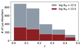
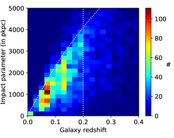
Figure 1: Top: Redshift distribution of number of Ly$\alpha$ absorbers in the sample used in this work. We present this for two H i column density thresholds. Bottom: 2D histogram plot of redshift vs. impact parameter of the complete galaxy sample along the quasar sightlines used in this study. The vertical dashed line denotes the maximum galaxy redshift used for our study. The dashed curve shows the projected length scale as a function of redshift for an angular scale of 20’.

We use a deep and wide galaxy redshift survey along 47 of HST-COS sightlines presented by Keeney et al. (2018) to probe the connection between Ly$\alpha$ clustering and galaxy distributions. We supplemented these data with the galaxies detected within 20’ to the quasar sightline from SDSS and Prochaska et al. (2011). 34 sightlines in Danforth et al. (2016) have galaxy information in Keeney et al. (2018). Five of these sightlines were also covered by Prochaska et al. (2011). We use the galaxy distribution around 8 other sightlines from Prochaska et al. (2011). Thus we have galaxy information around 41 sightlines in the sample of Danforth et al. (2016). In total we have 6174 galaxies close to these sightlines. In the bottom panel of of Fig. 1, the redshift and impact parameter distribution of these galaxies is shown. Vertical dotted line marks $z=0.2$. We also show the impact parameter corresponding to 20’. We use these data to find the properties of the nearest galaxies to the isolated absorbers and the absorbers showing strong two- and three-point redshift space (or velocity) correlation at $z\leq 0.2$. At $z\sim 0.1$ an angular scale of 20’ corresponds to a projected length scale of $\sim$2.3 pMpc. Apart from few cases the galaxy distribution from Keeney et al. (2018) is known to be complete for $\sim 0.1L*$ at $z<0.1$ and $L_{*}$ at z$\simeq$0.25. The data from Prochaska et al. (2011) also reach similar depth by over half the angular scale (i.e up to 10’ from the quasar sightline).

3 Absorber-based statistics

Maitra et al. (2019, 2020) presented two- and three-point correlation studies of Ly$\alpha$ forest using Voigt profile components as a suitable probe of the clustering properties of the IGM at $z>2$. These Voigt profile components can also be used to explore the connection between galaxies and intergalactic gas (see Rudie et al., 2012, for example). Throughout this paper, we will refer to these individual Voigt profile components as "absorbers". We will use the term absorption "system" to refer to the whole absorption profile. The Ly$\alpha$  absorber based approach allows us to study the two- and three-point correlations as a function of $N_{\rm HI}$, $b$ and presence of metals. In this section, we study the clustering properties of low-$z$ IGM by measuring longitudinal (i.e redshift space) three-point correlation of the Ly$\alpha$  absorbers. For doing so, we first estimate the $N_{\rm HI}$ distribution of the Ly$\alpha$  absorbers for the full sample and various sub-samples. This is an important first step to generate a set of mock sightlines having random distribution of Ly$\alpha$  absorbers that are used as a comparison to estimate the longitudinal three-point correlation. We also measure the longitudinal two-point correlation in order to estimate the reduced three-point correlation, Q.

3.1 Neutral hydrogen column density distribution

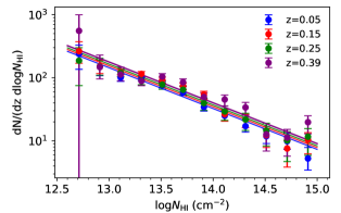
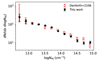
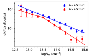
Figure 2: Top panel: $N_{\rm HI}$ distribution of Ly$\alpha$ absorbers for four different redshift intervals ($z=0.05\pm 0.05,\ 0.15\pm 0.05,\ 0.25\pm 0.05,\ 0.39\pm 0.09$). This plot confirms a weak redshift evolution of $f(N_{HI},z)$. Middle panel: comparison of the $N_{\rm HI}$ distribution obtained by us for the entire sample with that of Danforth et al. (2016). Bottom panel: The $N_{\rm HI}$ distribution for the low-$b$ ($b<40$ $kms^{-1}$) and the high-$b$ ($b>40$ $kms^{-1}$) sub-samples. In the case of high-$b$ sub-sample the distribution is well fitted by a double power-law. The double power-law fit to high-$b$ and single power-law fit to the low-$b$ samples are also shown.

In HST-COS spectra, the Signal-to-Noise Ratio (SNR) varies substantially across the observed wavelength range for a given sightline. So, the detectibility of any absorption feature has a wavelength (or $z$) dependence. We need the intrinsic distribution of Ly$\alpha$ absorbers having different column densities ($N_{\rm HI}$) to construct the random distribution of the absorbers after appropriately taking into account the $z$-dependence of detectibility along each sightline.

Following the standard practice (see for example, Petitjean et al., 1993), we define neutral hydrogen column density ($N_{\rm HI}$) distribution $f(N_{\rm HI},z)$ as the number of Ly$\alpha$ absorbers having log$N_{\rm HI}$ in the range of log$N_{\rm HI}\pm d$log$N_{\rm HI}/2$ and lying within redshift interval of $z\pm dz/2$. Traditionally, this distribution is approximated by a power law of $N_{\rm HI}$ and $z$, i.e,

$$f(N_{\rm HI},z)=\frac{d^{2}N}{d{\rm log}N_{\rm HI}dz}={\rm C_{0}}(1+z)^{\gamma}{N_{14}}^{\beta}.$$ (1)

Here, $N_{14}$ is $N_{\rm HI}$ expressed in units of $10^{14}cm^{-2}$.

To calculate the intrinsic distribution of the absorbers, we account for the "incompleteness" of the data sample. For a given column density we calculate the required spectral SNR so that the absorption line produced can be detected at $>4\sigma$ level. We do so by using the curve of growth for a given $N_{\rm HI}$ and assuming a median b value (i.e 34 $kms^{-1}$ for the full sample). So for a given $N_{\rm HI}$ bin, only those pixels having the observed SNR greater than the SNR limit where the absorption can be detected above 4$\sigma$ level are identified. Then we consider only the wavelength range covered by such pixels (as demonstrated in Fig.4 of Gaikwad et al., 2017b) for the calculation of redshift path length $dz$ in Eq. 1 . We calculate the total redshift path length corresponding to a given $N_{\rm HI}$ bin by integrating over all the quasar sightlines.

The redshift path length calculated in this way takes care of incompleteness coming from regions having the observed SNR lower than what is required for detecting an absorption line in a certain $N_{\rm HI}$ bin. We find that 25%, 50% and 75% of the observed redshift path length is sensitive enough to detect absorbers having log $N_{\rm HI}=$12.68, 12.84 and 13.0, respectively. The corresponding values obtained by Danforth et al. (2016) are log $N_{\rm HI}=$12.77, 12.93 and 13.09. The minor differences come from the fact that while Danforth et al. (2016) considers all the $N_{\rm HI}$ measurements (including systems with measurements based on Ly$\beta$ absorption for which Ly$\alpha$ is not covered), we consider only systems where Ly$\alpha$ absorption is covered in the HST-COS spectra. Also we avoid regions around 6 known galaxies that were searched for CGM absorption (see Section. 2 for details).

In the top panel of Fig. 2, we plot $f(N_{\rm HI},z)$ in different ${\rm log}N_{\rm HI}$ bins for 4 different redshift intervals ($z=0.05\pm 0.05$, $0.15\pm 0.05$, $0.25\pm 0.05$ and $0.39\pm 0.09$). The error in the distribution is one-sided poissonian uncertainty in the number of absorbers corresponding to $\pm 1\sigma$ computed over all the sightlines in a redshift bin. In the error, we also account for the uncertainty in $dz$ sourcing from the variation of completeness limit for a finite $N_{\rm HI}$ bin width. We then fit $f(N_{\rm HI},z)$ according to Eq. 1. The fitted parameter values are $\rm C_{0}=31\pm 2$, $\beta=-0.65\pm 0.03$ and $\gamma=0.7\pm 0.3$. The $C_{0}$ and $\gamma$ values are similar to $f(N_{\rm HI})=(167)N_{13}^{-0.65\pm 0.02}\approx(37)N_{14}^{-0.65\pm 0.02}$ reported in Shull et al. (2015), $f(N_{\rm HI})=(23\pm 1)N_{14}^{-0.67\pm 0.01}$ reported in Danforth & Shull (2008) and $f(N_{\rm HI})=(25\pm 1)N_{14}^{-0.65\pm 0.02}$ reported in Danforth et al. (2016) considering no redshift evolution in $N_{\rm HI}$ distribution. As seen in Fig. 2, $f(N_{\rm HI},z)$ depends strongly on the $N_{\rm HI}$ of the absorber while having a weak dependence on $z$ in the redshift range probed. For a sanity check, we compare this distribution with the one obtained in Danforth et al. (2016) in the middle panel of Fig. 2 and find them to be similar within measurement uncertainties. One caveat which needs to be mentioned is that while Danforth et al. (2016) calculate the $N_{\rm HI}$ distribution for the entire H i sample, we only do so for the H i Ly$\alpha$ absorbers which we use for this study. Our computed errors match well with those of Danforth et al. (2016).

In the bottom panel of Fig. 2, we plot $N_{\rm HI}$ distribution in two different bins based on $b$-values (high-$b$ sample with $b>40$ $kms^{-1}$ and low-$b$ sample with $b<40$ $kms^{-1}$) considering systems in the full sample. The cut-off $b$-value of 40 $kms^{-1}$ was chosen to delineate the possible BLAs from rest of the Ly$\alpha$ absorbers as defined in Lehner et al. (2007). About 31.9% of the total Ly$\alpha$ absorbers in our sample have $b>40$ $kms^{-1}$. In both cases, we recalculated the redshift path length considering the median $b$-values of the sub-samples. It is evident that both distributions have similar slope at low H i column density end (i.e., log $N_{\rm HI}$ $<10^{14}$ cm^-2) . However, we do notice a fall in the number of high-$b$ systems at high $N_{\rm HI}$ end. We fit the individual distribution using the form given in Eq. 1 ignoring the redshift evolution. The best fit values of $C_{0}$ and $\beta$ for low-$b$ and high-$b$ sub-samples are $C_{0}=23.0\pm 1.5,\ \beta=-0.60\pm 0.02$ and $C_{0}=9.5\pm 1.0,\ \beta=-0.83\pm 0.04$ respectively. In case of the high-$b$ sub-sample, we also fit the distribution with a double power law about $N_{\rm HI}=10^{13.5}$cm^-2 and obtain $C_{0}=22.1\pm 2.4,\ \beta=-0.44\pm 0.07$ for $N_{\rm HI}<10^{13.5}$cm^-2 and $C_{0}=12.4\pm 1.3,\ \beta=-0.95\pm 0.08$ for $N_{\rm HI}>10^{13.5}$cm^-2. We use these fitted distribution (i.e in general a single power-law fit and double power-law in the case of high-$b$ sub-sample) to generate the random distribution of absorbers.

3.2 Longitudinal two-point correlation function

We follow a standard procedure for finding the longitudinal two-point correlation function of Ly$\alpha$ absorbers. We calculate the probability excess of finding a pair of absorbers in the observed data relative to finding them in a random distribution of absorbers at certain redshift space separation. We select absorbers above a given $N_{\rm HI}$ threshold along the sightlines and estimate the longitudinal two-point correlation using the estimator,

$$\xi(r_{\parallel})=\frac{<DD>}{<RR>}-1\ ,$$ (2)

where "DD" and "RR" are the data-data and random-random pair counts of absorbers respectively at a separation of $r_{\parallel}$ (see Kerscher et al., 2000). Our choice of a normal estimator for two-point correlation is motivated by the fact that the clustering amplitudes are relatively independent of the choice of estimators at small scales, as shown in Kerscher et al. (2000). We checked and found that it holds for Ly$\alpha$ absorbers at the scales of interest in this study. Same is true for three-point correlation too (see Eq. 5). So, choose to go with the normal estimators as they save the computational time significantly (especially in the case of three-point correlation). The total data-data pairs $DD$ are summed over all the sightlines in their respective $r_{\parallel}$ bins and then normalized with $n_{D}(n_{D}-1)$ (where $n_{D}$ is the total number of absorbers). We use 100 random sightlines for every data sightline to minimize the variance in random. All the random pair counts for a given separation $r_{\parallel}$ are also normalized with total number of pair combinations ($n_{R}(n_{R}-1)$).

First, the distribution of absorbers along the random sightlines are generated using the best fitted power-law given by Eq. 1 for an observed sightline of length $dz$. We consider the random sightlines to have the same redshift range and same wavelength dependent SNR as the observed data. We compute the expected intrinsic number of random absorbers to be populated along the sightline (i.e. $N_{\rm abs}(R)$) by integrating Eq. 1 along the redshift pathlength and over the $N_{\rm HI}$ range in consideration,

$$N_{\rm abs}(R)=\int_{z_{l}}^{z_{u}}\int_{N_{\rm HI,l}}^{N_{\rm HI,u}}f(N_{\rm HI},z)~{}dz~{}d{\rm log}N_{\rm HI}.$$ (3)

Here, $z_{l}$ and $z_{u}$ are the minimum and maximum $z$ along the sightline respectively. $N_{\rm HI,l}$ is the lower $N_{\rm HI}$ threshold for the absorbers to be considered and we fix the upper limit $N_{\rm HI,u}$ to be $10^{18}$cm^-2. Next, we populate $N_{\rm abs}(R)$ number of random absorbers along the redshift path length by generating $N_{\rm abs}(R)$ randoms from the probability distribution of $(1+z)^{\gamma}$. For each of these randomly generated absorbers, we associate a random $N_{\rm HI}$ by drawing samples from the distribution $N_{\rm HI}^{\beta}$. Using the observed SNR, at the location of each randomly generated absorber, we compute the detection significance of the absorption line it will produce assuming the doppler width to be the median $b$ of the sample. Only lines with detection significance above 4$\sigma$ (similar to what has been used for the observations) are considered for the clustering analysis. In this way we account for the bias coming from non-uniform SNR across the spectrum.

We compute the two-point correlation logarithmically spaced $r_{\parallel}$ bins of [0.5-1, 1-2, 2-4, 4-8, 8-16, 16-32, 32-64] pMpc. We have taken this binning scheme specifically for the calculation of reduced three-point correlation function (see Eq. 6). We compute three-point correlation for collinear triplet configurations, which we explain in the next subsection. For such configurations, the third arm of the triplet will be double the length of the other two arm lengths. So, we take the $r_{\parallel}$ bins such that the mean of the next bin value is exactly double that of the previous bin value. This makes calculation of the cyclic combination of two-point correlations, $\overline{\xi(r_{1})}\times\overline{\xi(r_{2})}+\overline{\xi(r_{2})}\times\overline{\xi(r_{3})}+\overline{\xi(r_{1})}\times\overline{\xi(r_{3})}$ (see Eq. 6), necessary for calculating the reduced three-point correlation at each bin easier.

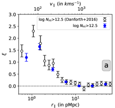
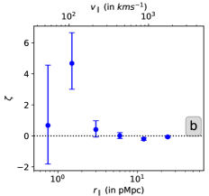
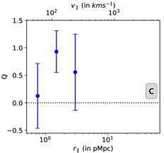
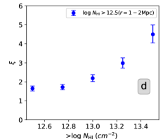
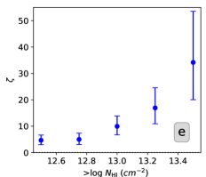
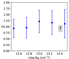
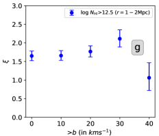
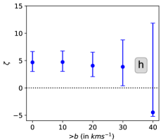
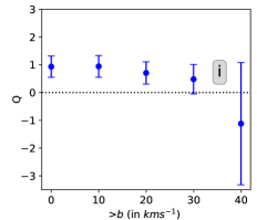
Figure 3: Absorber-based longitudinal two-point, three-point and Q (left to right) of Ly$\alpha$ absorbers as a function of longitudinal scale (top panels), $N_{\rm HI}$ thresholds (middle panels) and $b$ thresholds (bottom panels) . We consider $r_{\parallel}$ = 1-2 pMpc scale to probe the $N_{\rm HI}$ and $b$ dependence. The errors represent one-sided poissonian uncertainty corresponding to $\pm 1\sigma$ about the mean value. In panel (a) we compare our measurements with those of Danforth et al. (2016) for consistency check. Our measurements of two-point and three-point correlation as a function of longitudinal scale is provided in Table 1.

In panel (a) of Fig. 3, we plot the average two-point correlation of absorbers with $N_{\rm HI}>10^{12.5}$cm^-2 for our full sample as a function of $r_{\parallel}$. The error in the longitudinal two-point correlation is one-sided poissonian uncertainty corresponding to $\pm 1\sigma$ for all the data-data pairs. The uncertainty in the pairs for the large number of random absorbers taken is assumed to be relatively negligible. For a sanity check of our method, we compare our measurements with those of Danforth et al. (2016). The two-point correlation profile matches well within the errorbars (see panel (a) in Fig. 3). Our two-point correlation measurements are given in Table 1.

There are three scales of interest for longitudinal two-point correlation. At smaller scales ($r_{\parallel}<1.0$ pMpc), we observe a suppression in the two-point correlation. This region of suppression for Ly$\alpha$ absorbers is affected by thermal broadening along with instrumental resolution which sets a lower limit on scale for identification of multiple Ly$\alpha$ absorption lines during Voigt profile decomposition. We also expect pressure broadening and small scale clustering (and turbulence) of the baryonic gas to play a part in absorber suppression at smaller scales. At intermediate scales ($1.0$ pMpc$\leq r_{\parallel}\leq 6$ pMpc), longitudinal two-point correlation falls steadily and becomes consistent with zero beyond 10 pMpc.

Next we explore the $N_{\rm HI}$ dependence of $\xi$ in panel (d) of Fig 3. Here we mainly focus on the $r_{\parallel}$ bin of 1-2 pMpc. Consistent with the past studies, the amplitude of the two-point correlation steadily increases with increasing $N_{\rm HI}$ threshold (see for example, Penton et al., 2002; Danforth et al., 2016). As mentioned in the introduction, there is a strong correlation between $N_{\rm HI}$ and over-density. Therefore, $N_{\rm HI}$ dependence of clustering reflects the stronger clustering of more over-dense regions (See Maitra et al., 2020, for discussions on this related to high-z IGM). It is known that stronger Ly$\alpha$ absorbers (i.e with $N_{\rm HI}>10^{14}$cm^-2) at low-$z$ are clustered strongly with the galaxies while the weaker absorbers are distributed more randomly or associated with galaxy voids or IGM (Penton et al., 2002; Tejos et al., 2014). Therefore, increase in two-point correlation with $N_{\rm HI}$ threshold, could imply a stronger spatial clustering of Ly$\alpha$ absorbers associated with environments of galaxies.

3.3 Longitudinal three-point correlation function

The probability excess of finding a triplet of Ly$\alpha$  absorbers in the observed data in comparison to a random distribution of absorbers can be used to estimate the longitudinal three-point correlation function. However, the two-point correlations associated with the three arms of the triplet need to be subtracted from this probability excess to get the true three-point correlation function (see Eq. 5). The triplets are defined as three collinear points along a sightline having separations $r_{\parallel,1}$ between the first and second points and $r_{\parallel,2}$ between the second and third points. In this work, we mainly consider the equal length configuration $r_{\parallel,1}=r_{\parallel,2}=r_{\parallel}$ (within the assumed bin-intervals) . Our spatial separation measurements between the absorbers using the redshift difference is influenced by peculiar velocities. We address the effect of peculiar velocities on our measurements using simulated spectra in Section  5.

The probability excess of Ly$\alpha$ triplets with a separations of $r_{\parallel}$, $\rm PE_{3}$, is calculated for absorbers above a certain $N_{\rm HI}$ threshold using,

$$\rm PE_{3}=\frac{<DDD>}{<RRR>}-1,$$ (4)

where "DDD" and "RRR" are the data-data-data and random-random-random triplet counts. The $\rm PE_{3}$ is related to the three point correlation function, $\zeta(r_{\parallel})$, by

$$\zeta(r_{\parallel})={\rm PE_{3}}-\xi(r_{1})-\xi(r_{2})-\xi(r_{3})\ ,$$ (5)

where $\xi(r_{1}),\xi(r_{2})$ and $\xi(r_{3})$ are the two-point correlations for arm lengths joining the three points considered for three-point correlation (see Eq. 18 and 20 of Peebles & Groth, 1975). Similar to the two-point correlation, all the triplet counts at a certain separation $r_{\parallel}$ is normalized with total number of triplet combination. The $\rm PE_{3}$ and $\zeta$ for each data sightlines is calculated using 1000 random sightlines. The distribution of random absorbers along the sightlines and assignment of their $N_{\rm HI}$ values are done in a similar fashion as described earlier. The three-point correlation is also computed in logarithmically spaced $r_{\parallel}$ bins as explained above. In panel (b) of Fig. 3 we plot three-point correlation for $N_{\rm HI}>10^{12.5}$cm^-2 absorbers.

We measure positive three-point correlation (and probability excess) at scales below 4 pMpc (i.e line of sight velocity scales $<300$ $kms^{-1}$). At the scale of 1-2 pMpc, we have the strongest detection in three-point correlation (probability excess of $8.8^{+2.0}_{-1.7}$ and the corresponding three-point correlation of $\zeta=4.8^{+2.0}_{-1.7}$ at $\sim 2.6\sigma$ significance level). The amplitude of the three-point correlation in this $r_{\parallel}$ bin is higher than the corresponding two-point correlation. Similar to two-point correlation, we see the effects of suppression at scales below 1 pMpc. In panel (e) of Fig. 3, we plot $\zeta$ for different $N_{\rm HI}$ thresholds for the scale 1-2 pMpc. While a trend of increasing $\zeta$ with $N_{\rm HI}$ is evident, the measurement errors are large at high $N_{\rm HI}$ end due to small number of high $N_{\rm HI}$ absorbers involved. Our measurement of the probability excess and three-point correlation function as a function of longitudinal scale is provided in Table 1.

Next, we estimate the reduced three-point correlation Q for Ly$\alpha$  absorbers, which is defined as the three-point correlation normalized with cyclic product of two-point correlations (along the three arms connecting the three points considered for three-point correlation) as,

$$Q=\frac{\overline{\zeta(r_{1},r_{2},r_{3})}}{\overline{\xi(r_{1})}\times\overline{\xi(r_{2})}+\overline{\xi(r_{2})}\times\overline{\xi(r_{3})}+\overline{\xi(r_{1})}\times\overline{\xi(r_{3})}}\ ,$$ (6)

where $r_{1},r_{2}$ and $r_{3}$ are the arm lengths joining the three points considered for three-point correlation. For the longitudinal three-point correlation considered in this study, $r_{1}=r_{2}=\Delta r_{\parallel}$ and $r_{3}=2\times\Delta r_{\parallel}$ (see Groth & Peebles, 1977; Peebles, 1980). In panel (c) of Fig. 3, we plot the reduced three-point correlation Q as a function of longitudinal separations. We plot only up to a length scale of 4 pMpc because beyond that, we observe negligible three-point correlation. We find a Q value of $0.95^{+0.39}_{-0.38}$ at $r=1-2$ pMpc. In the $r=2-4$ pMpc bin, the Q value is found to be similar with larger errorbars. At $r<1$ pMpc, Q value is found to be negligible. We notice similar trend even when we consider only Ly$\alpha$  absorbers with $N_{\rm HI}$$>10^{13.5}$ cm^-2. In panel (f) of Fig. 3, we plot Q as a function of $N_{\rm HI}$ thresholds (for $r_{\parallel}=$ 1-2 pMpc bin) . The value of Q remains nearly constant with increasing $N_{\rm HI}$ thresholds albeit with large error bars. In section 5, we will compare the Q values predicted by the simulations with the observed values.

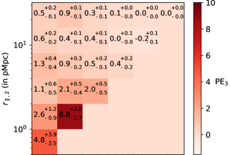
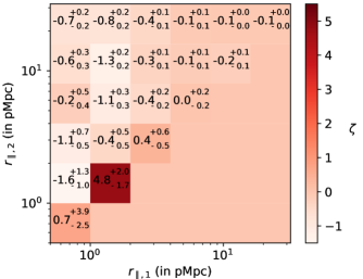
Figure 4: 2D-plot of absorber-based longitudinal probability excess of Ly$\alpha$ triplets (top) and three-point correlation (bottom) as a function of scales $r_{\parallel,1}$ and $r_{\parallel,2}$. The measured values of $\rm PE_{3}$ and $\zeta$ with errors are provided in each bin.

Till now we have considered the case of equal length configuration (i.e $r_{\parallel,1}=r_{\parallel,2}=r_{\parallel}$) . In Fig 4, we show the distribution of probability excess and three-point correlation for the case of $r_{\parallel,1}\neq r_{\parallel,2}$ for $N_{\rm HI}>10^{12.5}$cm^-2. Among the off-diagonal elements the bins with $r_{\parallel,1}=0.5-1.0$ pMpc and $r_{\parallel,2}=1.0-2.0$ pMpc and with $r_{\parallel,1}=1.0-2.0$ pMpc and $r_{\parallel,2}=2.0-4.0$ pMpc show a probability excess of $\sim 2$ at more than 2.5$\sigma$ level. However, none of these bins have significant non-zero three point correlation. Guo et al. (2016) have presented three point correlation function of galaxies for different configurations for 1:2 arm length ratio. Their result for $\theta\simeq 0$ (i.e squeezed configuration) will correspond to our equal arm configuration. It is evident from their measurements that $\zeta$ of Ly$\alpha$ forest is at least an order of magnitude smaller than what has been seen for galaxies for the same scales. In terms of velocity scale, the length over which one sees significant three point correlation function (i.e $\simeq$ 1-2 pMpc or 146 $kms^{-1}$in the velocity scale at the median redshift i.e $z\sim 0.15$ of our sample) is consistent with the velocity dispersion of gas clouds in high mass galactic halos. Conversely, this can also correspond to the large-scale structures in real space. So it is important to explore how much contribution to the observed three point correlation comes from CGM (see section 4) .

Table 1: Observed values of longitudinal two-point ($\xi$), triplet probability excess ($\rm PE_{3}$) and three-point ($\zeta$) correlations.

$r$		$\xi$		$\rm PE_{3}$		$\zeta$
(in pMpc)	(in $kms^{-1}$)	$N_{\rm HI}>10^{12.5}$cm-2	$N_{\rm HI}>10^{13.5}$cm-2	$N_{\rm HI}>10^{12.5}$cm-2	$N_{\rm HI}>10^{13.5}$cm-2	$N_{\rm HI}>10^{12.5}$cm-2	$N_{\rm HI}>10^{13.5}$cm-2
$0.5-1$	36.3-72.6	$1.20^{+0.18}_{-0.16}$	$3.65^{+0.68}_{-0.60}$	$4.77^{+3.87}_{-2.47}$	$-1.00^{+32.11}_{-0.00}$	$0.72^{+3.89}_{-2.49}$	$-12.81^{+32.14}_{-1.28}$
$1-2$	72.6-145.3	$1.65^{+0.13}_{-0.13}$	$4.50^{+0.49}_{-0.45}$	$8.76^{+1.96}_{-1.65}$	$44.33^{+19.34}_{-14.09}$	$4.76^{+1.98}_{-1.67}$	$34.18^{+19.36}_{-14.12}$
$2-4$	145.3-290.6	$0.70^{+0.07}_{-0.07}$	$1.14^{+0.22}_{-0.20}$	$1.98^{+0.54}_{-0.46}$	$7.76^{+4.32}_{-3.03}$	$0.41^{+0.56}_{-0.48}$	$4.88^{+4.34}_{-3.06}$
$4-8$	290.6-581.1	$0.18^{+0.04}_{-0.04}$	$0.59^{+0.13}_{-0.12}$	$0.37^{+0.18}_{-0.16}$	$2.66^{+1.32}_{-1.00}$	$0.01^{+0.20}_{-0.18}$	$1.31^{+1.35}_{-1.04}$

3.4 Dependence of clustering on $b$-parameter

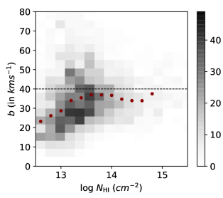
Figure 5: 2D histogram of $N_{\rm HI}$ vs. $b$ distribution. The horizontal dashed line at $b=40$ $kms^{-1}$demarcates the high-$b$ and low-$b$ sub-samples. Dots provides the median $b$ value in each $N_{\rm HI}$ bin. A correlation is seen between $N_{\rm HI}$ and $b$ for small values of $b$ and median $N_{\rm HI}$ is flat at large-$b$ values.

We have seen that Ly$\alpha$ clustering depends on $N_{\rm HI}$ and is stronger for higher $N_{\rm HI}$ absorbers. Here, we explore the dependence of Ly$\alpha$ clustering on $b$-parameter. Purely based on the existence of $N_{\rm HI}$ $vs.$ $b$ correlations we expect the absorbers with high $b$-values to cluster more strongly. Additionally, this exercise is motivated by the finding of Wakker et al. (2015), that the BLAs tend to have low impact parameter (i.e $\rho\leq 400$ pkpc) with respect to the filament axis compare to the narrow Ly$\alpha$ absorbers that are found up to $\rho\sim 3$ pMpc. Tejos et al. (2016) have also found the number of BLA absorption associated with the filaments are $\sim 6$ times in excess of random expectations. These absorbers may trace the warm ionized gas in the intracluster filaments.

Fig. 5 shows the scatter plot for the $N_{\rm HI}$ $vs.$ $b$ distribution in our sample. In our sample, 31.9% of the Ly$\alpha$ components have $b\geq 40$ $kms^{-1}$. It is also evident from this figure that the distribution of $N_{\rm HI}$ seems different for high-$b$ and low-$b$ sub-samples. High-$b$ sub-sample seems to have less number of high $N_{\rm HI}$ (as also seen in Fig. 2) . This is similar to the finding of Lehner et al. (2007) based on smaller number of sightlines. While one expects bias against detecting low $N_{\rm HI}$ high-$b$ absorbers when the SNR is low, lack of high-$b$ high $N_{\rm HI}$ absorption can be either physical or systematic bias introduced by the multiple component Voigt profile fits that tend to fit saturated lines with more narrow components.

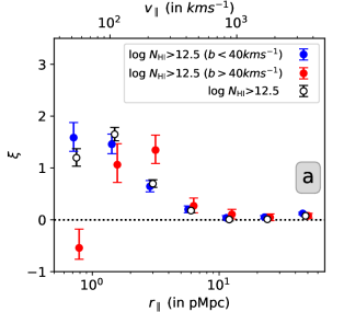
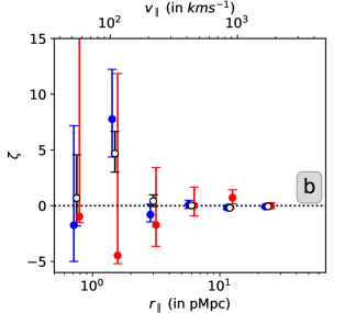
Figure 6: Two-point (panel a) and three-point (panel b) correlations of Ly$\alpha$ absorbers as a function of longitudinal scale for full sample as well as high-$b$ ($b>40$ $kms^{-1}$) and low-$b$ ($b<$ 40 $kms^{-1}$) sub-samples. The errors represent one-sided poissonian uncertainty corresponding to $\pm 1\sigma$ about the mean value. The results for the low-$b$ sample roughly follow the that of the whole sample. In the case of high-$b$ sub-sample, we do not find any triplets for $r_{\parallel}<4$ pMpc, this coupled with the low random probability to find high-$b$ triplets at these scale leads to large errors in $\zeta$.

In panel (g) of Fig. 3, we plot the two-point correlation function measured at $r_{\parallel}$ = 1-2 pMpc (equal arm configuration) as a function of different $b$-parameter thresholds. For generating the random distributions, as discussed in section 3.1, we compute the intrinsic $N_{\rm HI}$ distribution separately using appropriate median $b$ values for each sub-sample. Initially, we see a nearly constant two-point correlation with increase in $b$-parameter values. However, when we consider high-$b$ systems (i.e $b>40$ $kms^{-1}$) we notice that the two-point correlation function decreases. From panel (h) of Fig. 3, we find that the three-point correlation function also shows similar trend with a sharp decline in the amplitude for $b>40$ $kms^{-1}$ case ( with large errorbar). The same trend is also shown by $Q$ that we plot in the panel (i) of Fig. 3. We do not find any triplets with all the components having $b>40$ $kms^{-1}$ in $r_{\parallel}=1-2$ pMpc bin which results in a large negative mean three-point correlation. This could be real or artefact of some bias in the Voigt profile decomposition, in particular at small scales. For example, presence of a broad absorber can conceal other broad components from being detected within the scales considered here (in particular when the SNR is not high), thereby lowering the two-point and three-point correlations.

To see whether this is a scale dependent result, in Fig. 6 we plot the longitudinal two- and three-point correlations as a function of scale separately for high-$b$ and low-$b$ sub-samples for $N_{\rm HI}>10^{12.5}$ cm^-2. The random distribution of absorbers for each of these cases is drawn separately using the $N_{\rm HI}$ distributions shown in the bottom panel in Fig. 2. As can be seen from this figure, at $r_{\parallel}<2$ pMpc, the two-point correlation between the low-$b$ absorber (while consistent with the full sample) is stronger than that of high-$b$ absorbers. Over the same scale the high-$b$ absorbers show largely negative three-point correlation. This confirms the lack of triplets with large-$b$ values at small scales. This is consistent with what we have seen in Fig 3. However for the scales of 2-4 pMpc, we see a stronger two-point correlation for the high-$b$ sub-sample. In the case of three-point correlation function, contribution comes from a single triplet of high-$b$ absorbers ($b=$ 42.4 $kms^{-1}$, 144.3 $kms^{-1}$ and 51.2 $kms^{-1}$) seen along a single sight line (PKS 0405-123) at the redshift of 0.0251. For all other high $r_{\parallel}$ bins the low-$b$ and high-$b$ sub-samples have similar albeit with low values for correlation function. The trend seen for the two-point correlation is consistent with the suppression effects being severe in the case of high-$b$ absorbers for $r_{\parallel}<2$ pMpc and high-$b$ absorbers having higher $\xi$ at 2-4 pMpc. In the case of three-point, due to large errors we do not find any difference between high-$b$ absorbers and full sample for $r_{\parallel}>4$ pMpc.

3.5 Effect of presence of metal ions on correlation

$z<0.16$             $0.1<z<0.48$             $z<0.48$

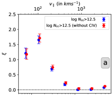
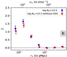
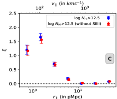
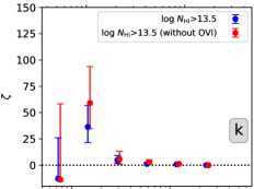
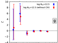
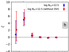
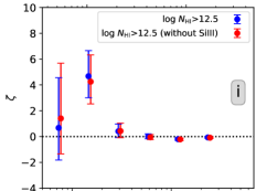
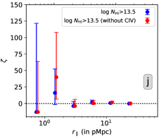
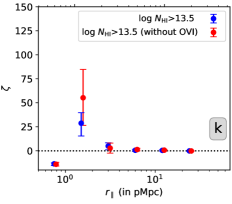
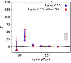
Figure 7: The top two rows show two-point correlation of Ly$\alpha$ absorbers with (blue) or without (red) associated metal lines such as C iv (left panels), O vi (middle panels) and Si iii (right panels) as a function of longitudinal scale for $N_{\rm HI}>10^{12.5}$cm^-2 (top row) and $N_{\rm HI}>10^{12.5}$cm^-2 (second most top row) . The bottom two panels show longitudinal three-point correlation in the same fashion. The errors represent one-sided poissonian uncertainty corresponding to $\pm 1\sigma$ around the mean value.

One important question which arises is that whether the correlations we detect originate from the IGM or are dominated by a small population of absorbers originating from CGM of intervening galaxies. Danforth et al. (2016) have shown that the metal bearing Ly$\alpha$ systems (based on the presence of O vi) show stronger two-point correlation than the non-metal bearing systems (see their figure 18). Based on this they concluded that most of the radial velocity clustering of the Ly$\alpha$ systems can be attributed to metal bearing systems originating from the CGM of intervening galaxies. Here, we ask a slightly different question. We would like to know whether the presence of different metal ion species influence the observed clustering properties of Ly$\alpha$ absorbers.

We base our study on C iv, O vi and Si iii metal line transitions. Considering the wavelength range covered by the HST-COS medium resolution spectrum, redshift ranges over which Ly$\alpha$, O vi and Si iii associated with the Ly$\alpha$ can be detectable are $z<0.16$, $0.1<z<0.48$ and $z<0.48$ respectively. So, for checking the dependence of Ly$\alpha$ clustering on the presence of C iv, O vi and Si iii  we consider redshift ranges of $z<0.16$, $0.1<z<0.48$ and $z<0.48$ respectively. We consider a metal line transition having redshift within the median $b$-parameter ($\sim 34$ $kms^{-1}$) of the redshift of Ly$\alpha$ absorbers to be associated with it. We only consider components with metal ion line absorption having rest equivalent width above 30 mÅ  (as done by, Danforth et al., 2016).

Firstly, we consider Ly$\alpha$ absorbers having $N_{\rm HI}>10^{12.5}$cm^-2. For $z<0.16$, 5.7% of such Ly$\alpha$ absorbers show detectable C iv absorption. For $0.1<z<0.48$, 19.8% of the Ly$\alpha$ absorbers show detectable O vi absorption. For $z<0.48$, 5.9% of the Ly$\alpha$ absorbers are associated with Si iii absorption. When we consider Ly$\alpha$ absorbers having $N_{\rm HI}>10^{13.5}$cm^-2, these percentages increase to 16.8% for C iv, 33.0% for O vi and 16.1% for Si iii. Note that for calculating these fractions, we have considered all metal ion line detections without applying any column density cut-off based on detection sensitivity.

In top two rows of Fig. 7, we plot the two-point correlation of “all Ly$\alpha$” absorbers and those “without associated metal ion species” absorption for the three identified metal ion species and two $N_{\rm HI}$ cut-offs. Note the “all Ly$\alpha$" sample in each of these cases is different owing to different redshift ranges probed (redshift ranges are provided on top of each column in Fig. 7). In the case of absorbers "without metal ion species” we just remove only the Voigt profile components that have associated metal absorption. As only a small fraction of Ly$\alpha$ absorbers will be removed based on the presence of metal ion species, we naively expect their influence to be minimal. However, we still draw appropriate random distributions of absorbers for each case separately while calculating $\xi$ and $\zeta$. For $N_{\rm HI}>10^{12.5}~{}{\rm cm}^{-2}$, the $\xi$ measured for systems without C iv, O vi and Si iii are consistent with their respective “all Ly$\alpha$” samples. This seem to be the case for $N_{\rm HI}>10^{13.5}~{}{\rm cm}^{-2}$ absorbers also. Therefore, it appears that two-point correlation function we measure for the Ly$\alpha$ absorption and its column density dependence may not originate mainly from the metal line bearing Ly$\alpha$ absorbers.

In bottom two panels of Fig. 7, we plot the three-point correlations for two $N_{\rm HI}$ cut-offs. The $\zeta$ does not show any significant difference between the full sample and the corresponding sample for Ly$\alpha$ without C iv, O vi or Si iii absorption. The three-point correlation measured for the Ly$\alpha$ absorbers does not source primarily from a metal line detected components.

3.6 Redshift Evolution

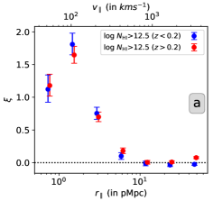
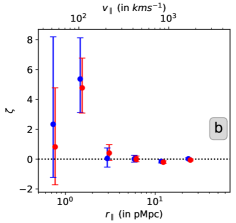
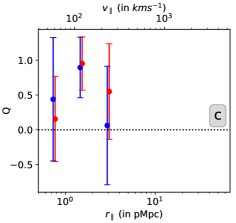
Figure 8: Two-point, three-point and reduced three-point correlation (left to right) of Ly$\alpha$ absorbers as a function of longitudinal scale for two different $z$-intervals. The errors represent one-sided poissonian uncertainty corresponding to $\pm 1\sigma$ about the mean value of correlations.

In this section, we investigate the redshift evolution of the two- and three-point correlation by considering two redshift bins $z<0.2$ and $0.2<z<0.48$ for $N_{\rm HI}>10^{12.5}~{}{\rm cm}^{-2}$. The choice of $z=0.2$ as a threshold between the two redshift bins is simply taken as the approximate midpoint of the redshift range of our sample. The left and middle panels in Fig. 8 show the $\xi$ and $\zeta$ respectively as a function of distance scale for the two sub-samples. It is clear from these two panels that the measured values of $\xi$ and $\zeta$ for the low-$z$ and high-$z$ sub-samples are consistent with each other within measurement uncertainties. We do not also find any difference in the Q profile for the two sub-samples (see right panel in Fig. 8) . Thus over the redshift range considered here we do not find any evolution in the amplitude of the two- and three-point correlation function.

4 Connection to galaxies

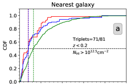
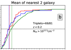
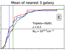
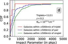
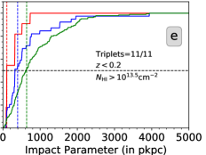
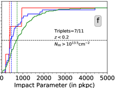
Figure 9: Cumulative distribution function (CDF) of impact parameter of galaxies associated with isolated or "singlet", "pair" (excluding the ones that are part of the triplets) and "triplet" Ly$\alpha$ absorbers. Left, middle and right columns show results of impact parameter for the nearest, average of two nearest and three nearest galaxies respectively. Number of the identified triplets have associated galaxy (or galaxies) is also provided in each panel. Results for log $N_{\rm HI}$$>$12.5 and 13.5 are given in the top and bottom rows respectively. The vertical dashed lines give the median value of impact parameter for each sub-sample.

Table 2: Galaxies nearby to identified Ly$\alpha$ absorber triplets.

QSO sightlines1	$z$ (Ly$\alpha$ triplet)	log $N_{\rm HI}$ of	$b$-parameter of	$v_{\parallel}$ (Nearest Galaxy-Ly$\alpha$ triplet )2	Impact parameter of Galaxy
		triplet system	triplet systems (in $kms^{-1}$)	(in $kms^{-1}$)	from sightlines2 (in pKpc)
Equal arm length configurations: $r_{\parallel}=0.5-1$ pMpc
PG1116+215B,M	0.1656	12.63, 13.39, 13.06	15.8, 30.7, 44.9	+98.3, -197.7, +312.0	156.0, 317.0, 531.4
PG1222+216B	0.1446	13.41, 13.32, 13.3	34.2, 18.6, 47.2	-956.9, -907.1, -941.2	1189.0, 1305.3, 1316.8
PKS2155-304B	0.1057	13.98, 13.33, 13.28	47.1, 21.6, 43.2	-265.1, +36.1, -34.5, +33.4	924.0, 952.0, 1025.0, 1094.0
Equal arm length configurations: $r_{\parallel}=1-2$ pMpc
H1821+643B	0.1217	14.21, 13.43, 13.14	38.1, 53.0, 38.1	-15.8, +273.1, -328.7	156.3, 1160.5, 1550.4
H1821+643B,M	0.1701	13.86, 13.68, 13.36	35.3, 58.0, 28.4	+127.7, +209.7, -369.7	415.4, 1122.2, 1118.7
H1821+643	0.1895	12.6, 12.72, 12.55	28.1, 26.1, 16.1	-140.0, -155.1, -84.5	1019.8, 1054.5, 1084.3
PG0953+414M	0.1423	12.73, 13.56, 13.48	15.3, 26.5, 30.9	+237.7, +78.0, +51.2	405.0, 452.1, 506.7
PG0953+414B,M	0.1426	13.56, 13.48, 13.2	26.5, 30.9, 52.7	+155.4, -4.2, -31.0	405.0, 452.1, 506.7
PG1048+342B,M	0.0061	14.8, 13.79, 13.99	42.7, 33.1, 86.9	-6.0, -167.0	60.2, 149.2
PG1048+342B,M	0.0057	14.07, 14.8, 13.79	30.4, 42.7, 33.1	+84.1, -77.0	60.2, 149.2
PG1116+215B	0.1658	12.63, 13.06, 14.28	15.8, 44.9, 32.7	+37.8 -258.1 +251.4	156.0, 317.0, 531.4
PKS0405-123B	0.0247	12.82, 12.56, 13.18	42.4, 13.4, 144.3	+1174.6, +1423.5, +1420.5	673.0, 799.0, 1105.0
PKS0405-123B	0.1527	13.44, 12.54, 13.79	25.8, 13.5, 47.8	132.0, 223.0, -445.8	181.0, 2148.0, 3857.0
Q1230+0115B,M	0.0948	12.99, 13.31, 14.33	69.7, 30.2, 46.3	+46.8, -16.1, +16.7	113.4, 792.3, 917.2
RXJ0439.6-5311B	0.1772	13.53, 13.6, 13.87	100.0, 19.7, 29.9	-65.8, -183.0, +127.9	467.2, 562.5, 1848.2
TON1187B	0.0354	13.38, 13.98, 13.59	18.9, 28.2, 56.4	+1398.9, +1149.7, +1346.8	278.1, 276.3, 284.1
Equal arm length configurations: $r_{\parallel}=2-4$ pMpc
H1821+643B	0.1899	12.6, 12.55, 12.73	28.1, 16.1, 41.6	-235.5, -250.6, -180.0	1019.8,1054.5,1084.3
H1821+643B	0.1901	12.55, 12.61, 12.73	16.1, 22.4, 41.6	+481.7,-287.1,-302.2	833.4,1019.8,1054.5
H1821+643B	0.1901	12.6, 12.61, 12.73	28.1, 22.4, 41.6	+481.7,-287.1,-302.2	833.4,1019.8,1054.5
H1821+643B	0.1908	12.55, 12.73, 12.57	16.1, 41.6, 15.9	+305.1, -463.3, -478.4	833.4,1019.8,1054.5
H1821+643B	0.1908	12.55, 12.73, 12.67	16.1, 41.6, 31.5,	+305.1, -463.3, -478.4	833.4,1019.8,1054.5
H1821+643B	0.1908	12.61, 12.73, 12.67	22.4, 41.6, 31.5	+305.1, -463.3, -478.4	833.4,1019.8,1054.5
H1821+643B	0.1908	12.61, 12.73, 12.57	22.4, 41.6, 15.9	+305.1, -463.3, -478.4	833.4,1019.8,1054.5
PG0953+414B	0.1914	12.91, 13.34, 13.27	25.2, 40.5, 55.3	0.0, -136.0	1232.6, 3692.8
PG1116+215B,M	0.1662	12.63, 14.28, 13.69	15.8, 32.7, 45.4	-53.5, -349.4, +160.0	156.0, 317.0, 531.4
PG1116+215B,M	0.1662	12.63, 13.39, 13.69	15.8, 30.7, 45.4	-53.5, -349.4, +160.0	156.0, 317.0, 531.4
PG1216+069B	0.1801	13.25, 13.52, 13.48	64.8, 53.3, 30.4	+140.8,-67.6, 214.5	588.6, 415.4, 632.0
PG1216+069B	0.1801	13.25, 13.52, 12.77	64.8, 53.3, 12.4	+140.8,-67.6, 214.5	588.6, 415.4, 632.0
PKS0405-123B	0.0251	12.82, 13.18, 13.11	42.4, 144.3, 51.2	+1051.2, +1300.0, +1297.0	673.0, 799.0, 1105.0
PKS0405-123B	0.1330	13.67, 13.22, 13.13	27.6, 24.2, 45.0	+227.7, +235.7, +156.2	467.0, 501.0, 714.0
PKS0405-123B	0.1522	12.97, 13.44, 13.79	21.8, 25.8, 47.8	+267.7, +358.8, -310.4	181.0, 2148.0, 3857.0
PKS0405-123B	0.1522	12.78, 13.44, 13.79	21.2, 25.8, 47.8	+267.7, +358.8, -310.4	181.0, 2148.0, 3857.0
PKS0558-504B	0.0280	14.08, 13.13, 13.61	32.2, 47.3, 55.1	-	-
Q1230+0115B,M	0.0057	13.68, 15.25, 13.25	24.4, 37.3, 42.8	+505.6, +595.1	155.1, 168.0

• Superscript B and M denotes presence of BLA and any metal ion species, respectively in at least one of the absorber in the triplet system.

  The triplets are organized according to the $r$ bin they belong to.

• The $v_{\parallel}$ and impact parameters of the nearest galaxies which have velocity separations larger than 500$kms^{-1}$ from the Ly$\alpha$ triplets have been highlighted in red.

Table 3: continued

QSO sightlines	$z$ (Ly$\alpha$ triplet)	log $N_{\rm HI}$ of	$b$-parameter of	$v_{\parallel}$ (Nearest Galaxy-Ly$\alpha$ triplet )	Impact parameter of Galaxy
		triplet system	triplet systems (in $kms^{-1}$)	(in $kms^{-1}$)	from sightlines (in pKpc)
$r_{1}=r_{\parallel},\ r_{2}=2r_{\parallel}$ configurations: $r_{\parallel}=0.5-1$ pMpc
3C263B,M	0.0633	13.92, 14.86, 15.24	27.5, 52.5, 41.0	-15.5, -131.2, -119.9	62.4, 571.5, 577.9
H1821+643B,M	0.1215	14.21, 13.49, 13.43	38.1, 35.6, 53.0	+40.9, +329.8, -272.0	156.3, 1160.5, 1550.4
H1821+643B,M	0.1217	13.49, 13.43, 13.14	35.6, 53.0, 38.1	-15.8, +273.1, -328.7	156.3, 1160.5, 1550.4
H1821+643	0.1899	12.72, 12.55, 12.61	26.1, 16.1, 22.4	-235.5, -250.6, -180.0	1019.8,1054.5,1084.3
PG0953+414B	0.0160	13.11, 13.48, 12.92	39.8, 54.2, 8.9	+102.8, -92.4	159.2, 454.5
PG0953+414B	0.0161	13.48, 12.92, 13.52	54.2, 8.9, 24.8	+64.4, -130.4	159.2, 454.5
PG1116+215B,M	0.1658	13.39, 13.06, 14.28	30.7, 44.9, 32.7	+37.8, -258.1, +251.4	156.0, 317.0, 531.4
PG1216+069B	0.1799	13.25, 13.98, 13.52	64.8, 33.6, 53.3	-7.4, +201.1, +274.9	415.4, 588.6, 632.0
PHL1811B,M	0.1205	13.01, 14.17, 13.8	77.4, 52.1, 19.6	-91.3, +425.4	1222.3, 1840.0
PKS0405-123B,M	0.1666	12.6, 13.54, 15.01	21.8, 29.3, 50.7	+116.2, -184.6, -364.7	115.0, 2472.0, 3177.0
PKS2155-304	0.0170	13.43, 13.53, 13.3	22.9, 24.5, 39.9	-25.4	113.0
PKS2155-304B	0.0542	13.85, 13.61, 12.75	34.9, 52.5, 23.7	-37.8	544.0
TONS210B	0.0858	13.05, 13.07, 12.91	73.0, 19.8, 19.5	-	-
$r_{1}=r_{\parallel},\ r_{2}=2r_{\parallel}$ configurations: $r_{\parallel}=1-2$ pMpc
3C263B,M	0.1137	14.06, 13.27, 13.87	46.4, 56.8, 22.1	+13.7, +8.4, +258.9	351.0, 689.4, 708.9
3C273B	0.0671	14.08, 12.6, 12.62	37.0, 73.6, 25.0	+2168.5	661.0
H1821+643M	0.1215	14.21, 13.49, 13.14	38.1, 35.6, 38.1	+40.9, +329.8, -272.0	156.3, 1160.5, 1550.4
H1821+643	0.1895	12.6, 12.72, 12.61	28.1, 26.1, 22.4	-140.0, -155.1, -84.5	1019.8, 1054.5, 1084.3
H1821+643B	0.1899	12.72, 12.55, 12.73	26.1, 16.1, 41.6	-235.5, -250.6, -180.0	1019.8, 1054.5, 1084.3
H1821+643B	0.1914	12.73, 12.57, 12.67	41.6, 15.9, 31.5	+149.8, +200.2, +159.9	833.4, 1301.0, 1847.2
HE0153-4520M	0.1489	13.34, 13.25, 12.98	35.6, 29.3, 26.0	-133.4, +229.5, -62.9	1079.3, 1085.2, 1477.9
HE0153-4520B,M	0.1706	12.66, 13.71, 14.33	32.9, 100.0, 39.6	-435.7, -64.1, -12.8	911.3, 2145.1, 2384.1
PG0953+414B	0.0160	13.11, 13.48, 13.52	39.8, 54.2, 24.8	+102.8, -92.4	159.2, 454.5
PG0953+414	0.0161	13.11, 12.92, 13.52	39.8, 8.9, 24.8	+64.4, -130.8	159.2, 454.5
PG0953+414B,M	0.1423	12.73, 13.56, 13.2	15.3, 26.5, 52.7	+237.7, +78.0, +51.2	405.0, 452.1, 506.7
PG0953+414B	0.1426	12.73, 13.48, 13.2	15.3, 30.9, 52.7	+155.4, -4.2, -31.0	405.0, 452.1, 506.7
PG1048+342B,M	0.0057	14.07, 14.8, 13.99	30.4, 42.7, 86.9	+84.1, -77.0	60.2, 149.2
PG1048+342B	0.0061	14.07, 13.79, 13.99	30.4, 33.1, 86.9	-6.0, -167.0	60.2, 149.2
PG1116+215B,M	0.1662	13.06, 14.28, 13.69	44.9, 32.7, 45.4	-53.5, -349.4, +160.0	156.0, 317.0, 531.4
PG1216+069B,M	0.1239	14.65, 14.6, 14.54	24.5, 28.4, 44.6	+56.1, -64.1, +184.2	88.0, 91.6, 389.0
PG1216+069M	0.1239	14.65, 14.6, 14.1	24.5, 28.4, 23.3	+56.1, -64.1, +184.2	88.0, 91.6, 389.0
PG1216+069B	0.1799	13.25, 13.98, 13.48	64.8, 33.6, 30.4	-7.4, +201.1, +274.9	415.4, 588.6, 632.0
PG1216+069B	0.1799	13.25, 13.98, 12.77	64.8, 33.6, 12.4	-7.4, +201.1, +274.9	415.4, 588.6, 632.0
PG1307+085B,M	0.1413	12.91, 13.92, 13.28	49.7, 34.0, 28.5	-245.5, -421.6	1318.0, 1408.0
PG1307+085B,M	0.1413	12.91, 13.92, 14.02	49.7, 34.0, 40.2	-245.5, -421.6	1318.0, 1408.0
PG1424+240B,M	0.1471	14.66, 14.74, 13.51	49.9, 38.3, 55.5	-121.6, +380.5, -464.2	493.2, 968.5, 1378.9
PKS0405-123B	0.0251	12.56, 13.18, 13.11	13.4, 144.3, 51.2	+1174.6, +1423.5, +1420.5	673.0, 799.0, 1105.0
PKS0405-123	0.1522	12.97, 13.44, 12.54	21.8, 25.8, 13.5	+267.7, +358.8, -310.4	181.0, 2148.0, 3857.0
PKS0405-123	0.1522	12.78, 13.44, 12.54	21.2, 25.8, 13.5	+267.7, +358.8, -310.4	181.0, 2148.0, 3857.0
PKS0405-123B,M	0.1829	14.61, 13.98, 12.7	43.7, 33.8, 36.7	-255.94, -149.4, -169.7	3854.0, 4017.0, 5395.0
PKS1302-102B,M	0.1925	14.47, 13.95, 13.64	34.0, 39.5, 54.8	-194.0, -22.9, +120.5	209.0, 434.0, 464.0
PKS1302-102M	0.1925	14.47, 13.95, 13.6	34.0, 39.5, 23.2	-194.0, -22.9, +120.5	209.0, 434.0, 464.0
Q1230+0115	0.0485	12.75, 13.49, 13.16	35.9, 29.9, 20.8	-95.3, -15.2, -158.2	912.3, 1104.2, 1148.3
Q1230+0115B	0.0554	12.56, 12.65, 12.92	20.7, 38.5, 56.7	+1559.4, +1673.1, +880.1	353.0, 517.0, 533.0
SBS1108+560B,M	0.1385	13.27, 15.25, 14.31	42.6, 23.9, 25.2	-89.3, -225.0, -429.3	336.3, 453.0, 465.2
SBS1122+594B	0.1375	13.34, 13.14, 13.63	77.6, 14.9, 100.0	-453.6, -97.6, -390.3	1299.2, 1488.3, 1759.1
SBS1122+594B	0.1381	13.14, 13.63, 13.84	14.9, 100.0, 150.0	-264.6, -53.8	1488.3, 2189.5
SBS1122+594	0.1578	13.4, 13.91, 13.27	33.4, 18.9, 21.3	-28.5, -261.7, -303.2	556.8, 633.4, 687.4

In this section,we study the connection between the Ly$\alpha$ absorbers that are isolated, pairs or triplets that contribute to the observed two- and three-point correlations with nearby galaxies in the sample discussed in Section 2. We have not considered the galaxies around 3C57 for our analysis due to poor completeness of the galaxy sample (see discussions in Keeney et al., 2018). We identify all the Ly$\alpha$ triplets with equal arm (for $r_{\parallel,1}\leq 4$ pMpc) and 1:2 configuration (for $r_{\parallel,1}\leq 2$ pMpc) at $z<0.2$ that are present along 41 sightlines having galaxy information. Triplets with such configurations are chosen because $\rm PE_{3}$ is detected significantly for these configurations (see Fig. 4) .

Details of the triplets and the associated galaxies are provided in Table 2. First four columns in this table give QSO name, absorption redshift of the central component of the triplet, column densities of individual components in the triplet system and the $b$-parameters of the components. Fifth column of this table gives the line of sight velocity separation for up to 3 nearest catalogued galaxies with respect to the absorption redshift (redshift of the central absorber). We define nearest galaxies by their transverse distance from the sightlines. We consider only those galaxies that are within $\pm$500 $kms^{-1}$. This velocity is chosen to account for the typical velocity dispersion in galaxies (i.e $\leq$350 $kms^{-1}$) and that of the Ly$\alpha$ triplets (i.e $\sim$300 $kms^{-1}$). Impact parameters of these galaxies ( the distance between the absorber and the galaxy measured using the angular separation between the QSO sightline and the galaxy) are provided in the last column. In eight cases we find nearest galaxies having velocities in the range 500 -2500 $kms^{-1}$(red colour entrees in Table 2) . We do not detect any nearby galaxy within 2500 $kms^{-1}$ for 2 triplets. We discuss these specific cases in detail below.

First we consider the "equal arm" configuration. There are three triplets in the $r_{\parallel}$ = 0.5-1.0 pMpc bin and two of them show associated galaxies. The impact parameter of these galaxies are 156 and 924 pkpc. In the third case the nearest cataloged galaxy has a velocity difference of $\sim$ 957 $kms^{-1}$ (and an impact parameter of $\sim$1.2 pMpc) with respect to the absorption redshift. All the three triplets have at least one component having $b>40$ $kms^{-1}$. Only one of these absorbers show detectable metals at $z=0.1656$ with the nearest cataloged galaxy at an impact parameter of 156 pkpc. Note that none of these systems satisfy the $N_{\rm HI}$ threshold of $10^{13.5}$cm^-2.

In the case of $r_{\parallel}$ = 1.0-2.0 pMpc bin (where we detect $\zeta$ with best significance level), there are thirteen triplets contributing to the three-point correlation. Eleven of them have at least one component having $b>40$ $kms^{-1}$and only six show detectable metal absorption with impact parameters to the nearest cataloged galaxies in the range 60-467 pkpc (see column 6 of Table. 2). There are two cases where the same absorber contributes twice to our triplet counts (i.e multiple component systems with two combinations consistent with our triplet definition). Therefore, there are eleven independent systems contributing to the triplet count. One of these systems also contribute to $r_{\parallel}$ = 0.5-1.0 pMpc. We find nine of these eleven independent systems identified here have nearby galaxies with velocity separations within $\pm$500 $kms^{-1}$. The impact parameter of the nearby galaxies varies from 60 pkpc to 1 pMpc with a median impact parameter of 181 pkpc. We notice that systems contributing multiple times to the three-point function tend to have low (i.e $<$500 pkpc) impact parameters. In the remaining two cases we do identify nearby galaxies but with large velocity separations (i.e between 1000-1500 $kms^{-1}$). Interestingly only two systems (three independent triplets) in this list satisfy $N_{\rm HI}$$\geq 10^{13.5}$ cm^-2. In both cases galaxies are found with velocity separations less than 200 $kms^{-1}$and impact parameter of the nearest galaxy $\leq$ 500 pkpc.

In the case of $r_{\parallel}$ = 2.0 - 4.0 pMpc bin there are eighteen triplets (originating from nine independent systems) contributing to the measured $\zeta$. In all these cases at least one of the components has $b>40$ $kms^{-1}$ and only three of them show detectable metal lines. For six of these independent systems we find galaxies with velocity separations within $\pm$500 $kms^{-1}$. In one case we identify galaxies having velocity separation just above the cut-off. In these six systems the measured impact parameters of the nearest galaxy in the range 0.156-1.102 pMpc with a median value of 833.4 pkpc. In one case we identify the nearest galaxy to have velocity separations of 1050 $kms^{-1}$and impact parameter of 673 pkpc. In one case we do not have any galaxies nearest to the absorbers. In the case of $z=0.0280$ triplet towards PKS 0558-504 the galaxy observations are complete up to 0.1 L*. However, the maximum impact parameter probed is $\sim$ 400 pkpc. Considering several of the associated galaxies for this configuration are at impact parameter $>400$ pkpc (see Table 2), we need to search for galaxies at slightly higher impact parameters before confirming this triplet as a void absorber. Interestingly, none of the triplets satisfy the $N_{\rm HI}$ threshold of 10^13.5 cm^-2 in this $r_{\parallel}$ bin. As discussed before, in only one triplet (i.e $z=0.0251$ towards PKS 0405-123), we find all the three components having $b>40$ $kms^{-1}$the nearest cataloged galaxies have velocity separations in excess of 1000 $kms^{-1}$and impact parameters in the range $673-1105$ pkpc.

Next we consider the configuration with an arm length ratio 1:2. In the $r_{\parallel,1}$ = 0.5-1 pMpc bin we identify thirteen triplets (and eleven independent systems). Eleven of these triplets show at least one of the components having $b>40$ $kms^{-1}$and only six of them show detectable metal absorption. We could identify at least one nearby galaxy in ten out of eleven independent systems. In these systems the nearest impact parameter ranges from 62 pkpc to 1.2 pMpc with a median value of 158 pkpc. For one triplet (i.e $z=0.08586$ towards TON S210) we do not detect any associated galaxy within 2500 $kms^{-1}$. The galaxy observations are deep enough to detect 0.1L* galaxy within an impact parameter of 960 pkpc. Most of the galaxies detected in other cases for this configuration are well within this impact parameter. Therefore, lack of galaxy identification could mean this triplet being a void absorber. Only one system satisfies the $N_{\rm HI}$ threshold of 10^13.5 cm^-2 and this happen to be the system with the lowest impact parameter in this $r_{\parallel,1}$ bin.

For the $r_{\parallel,1}$ = 1-2 pMpc bin we identify thirty-four triplets (from twenty-five independent systems). Out of this, twenty-four triplets have at least one component with $b>40$ $kms^{-1}$ and only sixteen triplets show detectable metal lines. We find thirty-one triplets having at least one nearby galaxy with velocity separation $<500$ $kms^{-1}$. For these triplets, the nearest impact parameter range from 60 pkpc to 3.8 pMpc with a median value of 410 pkpc. For three triplets, we find nearest galaxies with large velocity separations (1100-2200$kms^{-1}$) with the nearest impact parameters in the range of 350-660 pkpc. Only seven triplets satisfy $N_{\rm HI}$ threshold of 10^13.5 cm^-2 and all of these have nearby galaxies within a velocity separation of 200 $kms^{-1}$and with impact parameters ranging from 60 pkpc to 500 pkpc.

In summary, for five configurations considered here we identify at least one associated galaxy within a velocity separation of 500 $kms^{-1}$ for $\sim 88$% of the triplets. The measured impact parameters of the nearest galaxies range from 62-3800 pkpc with a median value of 405 pkpc. Therefore, a good fraction of triplets originate from impact parameters that are inconsistent with them being associated to a single galaxy. The occurrence of $b>40$ $kms^{-1}$ absorbers are more frequent among the triplets ($\sim 85$%, as opposed to the $31.9$% for isolated absorbers). However, in only one case we see all the three components having $b>40$ $kms^{-1}$. In only twenty-one cases ($\sim$25%) we have two components having $b>40$ $kms^{-1}$. Only 40% of all the triplets are associated with metal line absorption. Most of the triplets are originating form low $N_{\rm HI}$ systems with only $\sim$14% of the identified triplets having all components having $N_{\rm HI}$$\geq 10^{13.5}$ cm^-2.

Next we ask the question, is the impact parameter distribution for the triplets different from those of doublets and isolated absorption lines. For this we calculate the cumulative distribution function (CDF) of the impact parameters of respective sightlines from galaxies in three ways: first we consider the impact parameter of the nearest galaxy, second the average impact parameter of the 2 nearest galaxies (nearest in transverse direction) and third, the average impact parameters of the 3 nearest galaxies. If we do not find the minimum required number of galaxies, then we do not consider those cases. As above, we consider only galaxies which are within $\pm 500$$kms^{-1}$ of Ly$\alpha$ pairs (and $r_{\parallel}$ within 0.5-1, 1-2 and 2-4 pMpc) that do not belong to a triplet system. Similarly, we also identify galaxies which are within $\pm 500$ $kms^{-1}$ of isolated individual Ly$\alpha$ absorbers (singlet), which do not belong to either a triplet or a pair.

In Fig. 9, we plot the CDF of impact parameters of these galaxies associated with triplet, pair and singlet Ly$\alpha$ systems. The left, middle and right columns denote impact parameters considered for the nearest galaxy, average of two nearest galaxies and average of three nearest galaxies, respectively. Top panels are for $N_{\rm HI}$$>10^{12.5}$ cm^-2 case and the bottom panels are for $N_{\rm HI}$$>10^{13.5}$ cm^-2.

As discussed before for the $N_{\rm HI}$$>10^{12.5}$ cm^-2 case, the median impact parameter with the nearest galaxies for the triplets in our sample is 405.0 pkpc and the largest separation found is 3.8 pMpc. In the case of doublets (respectively singlets) the median impact parameter is 415.4 pkpc (respectively 645.1 pkpc) and the largest separation found is 3.8 pMpc (respectively 5.4 Mpc) . From panel (b) and (c) of Fig 9, we notice that 69 (i.e 85% triplets) and 56 (i.e 69% triplets) out of 81 triplets have at least two and three nearby galaxies with velocity separation $<500$ $kms^{-1}$. The median separations of two nearest galaxies are 658.4 pkpc, 608.9 pkpc and 796.2 pkpc for triplets, doublets and singlets respectively. While there is clear distinction in the median impact parameter for the single and multiple (i.e doublets plus triplets) Ly$\alpha$ absorbers, we do not find any significant difference between the median impact parameter of doublets and triplets. The median separation for three nearest galaxies are 953.5 pkpc, 651.9 pkpc and 931.5 pkpc for triplets, doublets and singlets respectively. Even though the median separation may seem similar between triplets and singlets, as can be seen below the KS test results suggest the two distributions are statistically different.

We perform KS-test to compare different CDFs and results are summarized in Table 4. Here D is the maximum separation between the two distributions and Prob(D) is the probability that this D occurs by chance. This table confirms that there is no statistically significant difference between the distribution of impact parameters for triplets and doublets. While the impact parameter distribution of singlet is significantly different from that of triplets.

Next we consider $N_{\rm HI}$$>$ $10^{13.5}$ cm^-2 case, we identify eleven triplets and all of them have nearby galaxies within line of sight velocity separation $<500$ $kms^{-1}$. All eleven triplets show $b>40$ $kms^{-1}$components and nine of them show detectable metals. In this case the median separations of these nearby galaxies are 88 pkpc, 256 pkpc and 459 pkpc for the triplets, doublets and singlets respectively. In this case it is possible that some of the correlated absorption may originate from the halos of individual galaxies. Impact parameters measured are systematically smaller than the corresponding values for $N_{\rm HI}$$>$ $10^{12.5}$ cm^-2. We also confirm this with KS-test. The D and Prob(D) values are 0.54 and 0.004 respectively.

As Keeney et al. (2018) also provide stellar mass and luminosities of individual galaxies we also searched for any differences in the observed luminosities and inferred stellar masses of nearest galaxies (as stated before, within a velocity separation of 500 $kms^{-1}$) associated with triplets compared to doublets and singlets. We do not find any strong trend. This may once again hint towards the idea that most of the Ly$\alpha$ absorbers studied here are not physically linked to individual galaxies. The results presented are consistent with the findings in previous studies that most Ly$\alpha$ absorbers originate from the filamentary structures with BLAs and multiple absorbers having low impact parameters to the filament axis compared to the low $N_{\rm HI}$ isolated absorbers (see Davé et al., 2001; Penton et al., 2002; Davé et al., 2010; Wakker et al., 2015; Tejos et al., 2016). The volume probed and the completeness level reached in terms of luminosity for the galaxy will not allow us to perform an investigation similar to Wakker et al. (2015). However, it will be possible to explore for some of the very low-$z$ triplets using SDSS data base. We leave that exercise to a future work.

Table 4: Results of KS-test

Case	log $N_{\rm HI}$	Triplet vs. doublet		Triplet vs. singlet		Doublet vs. singlet
	threshold	D	Prob(D)	D	Prob(D)	D	Prob(D)
Nearest neighbour	12.5	0.11	0.69	0.27	0.0001	0.23	0.0002
2 neighbours	12.5	0.10	0.77	0.23	0.002	0.18	0.013
3 neighbours	12.5	0.12	0.74	0.23	0.01	0.16	0.05
Nearest neighbour	13.5	0.36	0.15	0.56	0.001	0.23	0.04
2 neighbours	13.5	0.40	0.09	0.58	0.001	0.25	0.03
3 neighbours	13.5	0.27	0.71	0.46	0.08	0.23	0.09

5 Simulations

In this section, we study the clustering of Ly$\alpha$ absorbers using four hydrodynamical simulations for $z=0.1$. Main motivations for this exercise are: (i) to measure the two- and three-point correlation functions for different scales; (ii) to quantify the effect of redshift space distortions in the measurement of line of sight correlation functions, (iii) to see whether the observed dependence of $\zeta$, $\xi$ and Q on $N_{\rm HI}$ and $b$ are naturally realised in the simulations as well, and (iv) to see the effect of feedback (Wind and AGN) on the correlation functions. However, we do not make any attempt to fine tune the simulation parameters and/or various sub-grid physics used to reproduce the observations.

The MassiveBlack-II (MBII) hydrodynamic simulation (Khandai et al., 2015) was run in a 100$h^{-1}$ cMpc ( Mpc in comoving units) cubic periodic box with $2\times 1792^{3}$ particles using p-gadget which is a hybrid version of gadget-3 upgraded to run on Petaflop-scale supercomputers. This simulation used the UV background model of Haardt & Madau (1996) and incorporates feedback associated with star formation and black hole accretion and cosmological parameters from $(\Omega_{m}=0.275,\Omega_{\Lambda}=0.725,\Omega_{b}=0.046,h=0.702,\sigma_{8}=0.816,n_{S}=0.96)$ from WMAP7 (Komatsu et al., 2011).

We also use three hydrodynamical simulation boxes from publicly available Sherwood Simulation suite (Bolton et al., 2017) to explore the effect of wind and AGN feedback. All of them are performed in a 80 h^-1 cMpc cubic box with $2\times 512^{3}$ particle using P-Gadget-3 (Springel, 2005). The model “80-512" is run with quick_lyalpha (as described in Viel et al., 2005) command without any stellar or wind feedback. The second simulation “80-512-ps13" implements the star formation and energy driven wind model of Puchwein & Springel (2013), but without AGN feed back. The third simulation “80-512-ps13+agn" implements the AGN feedback in addition to the star formation and energy driven wind models. All three simulations have the same initial seed density field, utilize Haardt & Madau (2012) UV background and use the same set of cosmological parameters from Planck Collaboration et al. (2014), where $\Omega_{m}=0.308,\Omega_{\Lambda}=0.692,\Omega_{b}=0.0482,h=0.678,\sigma_{8}=0.829,n_{S}=0.961$. Nasir et al. (2017) provides a detailed comparison of predictions of these three models with observations.

Recent studies (see Kollmeier et al., 2014; Shull et al., 2015; Khaire & Srianand, 2015; Gaikwad et al., 2017a, b) have shown that the H i ionization rate ($\Gamma_{\rm HI}$) at $z\sim 0.1$ is higher than those predicted by Haardt & Madau (2012). Therefore, for calculating the H i density fields from the simulations, we use the $\Gamma_{\rm HI}$ at $z\sim 0.1$ from Khaire & Srianand (2019) uniformly for all the simulations. We do not adjust $\Gamma_{\rm HI}$ to match the mean flux with observations. We generate 4000 lines of sight through these boxes using standard procedure described in our earlier papers (Gaikwad et al., 2017b; Maitra et al., 2020; Gaikwad et al., 2020a). We find the mean transmitted flux of 0.973, 0.979, 0.977 and 0.978 for MBII, 80-512, 80-512-PS13 and 80-512-PS13+AGN simulations respectively. These are close to what is observed, i.e, 0.961 for the full sample and 0.967 for the Ly$\alpha$ absorption at $z<0.2$. We convolve the spectrum with a gaussian profile with FWHM=17 $kms^{-1}$(instead of using HST line spread function), add a gaussian noise corresponding to SNR$=$50 per pixel and use spectral sampling (i.e $\sim$5 $kms^{-1}$ per pixel) similar to the HST-COS spectra. The usage of Gaussian LSF is justified as observationally what we have is the deconvolved $b$-distribution. We use high SNR spectra to get an insight into the intrinsic clustering of the Ly$\alpha$ absorbers. Simulated spectra are fitted with multiple Voigt profile components using VIPER (see Gaikwad et al., 2017b, for details). As in the observations, we consider only components that satisfy rigorous significant level in excess of 4 for our analysis.

5.1 Distributions of $b$-parameter and $N_{\rm HI}$

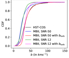
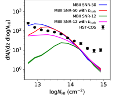
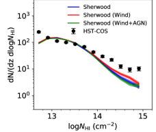
Figure 10: Left panel: Cumulative distribution function for $b$-parameter for MBII simulations (for two SNR) are compared with the observed distribution. Simulations tend to produce low-$b$ values compared to the observed distribution. Addition of $b_{\rm turb}$ reduces this difference. Our high SNR model produces over all CDF closer to the observed distribution. Middle panel: $N_{\rm HI}$ distribution predicted by MBII simulations are compared with the observed distribution. The high SNR simulation predicts a larger number of low $N_{\rm HI}$  absorbers in comparison to observations. The number goes down with the addition of $b_{\rm turb}$ in the low $N_{\rm HI}$ end. The low SNR simulations produce significantly lesser low $N_{\rm HI}$  absorbers due to incompleteness. On the high $N_{\rm HI}$ ends, the simulations produce significantly lesser absorbers than the observations. Right Panel: $N_{\rm HI}$ distribution predicted by Sherwood simulations. Like MBII simulations, absorbers with $N_{\rm HI}$$>10^{14}$ cm^-2 are under-predicted. However, the low $N_{\rm HI}$ end matches relatively better than MBII simulations.

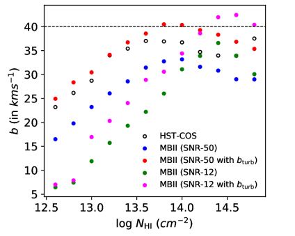
Figure 11: Median b-parameter in different $N_{\rm HI}$ bins obtained from our simulations are compared with observations. The horizontal dotted line at $b=40$ $kms^{-1}$demarcates the high-$b$ and low-$b$ sub-samples.

To begin with, we explore how well the simulations reproduce the observed $N_{\rm HI}$ and $b$ distributions. In panel (a) of Fig. 10, we compare the cumulative distribution function of the $b$-parameter of Ly$\alpha$ absorbers found in MBII simulation with the observed distribution. We find that the simulation produces lower $b$-values (median b of $\sim 25.0$ $kms^{-1}$) in comparison to the observations (median $b$ of $\sim 34.4$ $kms^{-1}$). Nasir et al. (2017) have found Sherwood simulations also to produce low-$b$ values. The median $b$-values are 24.4, 24.7 and 26.1 $kms^{-1}$for models 80-512, 80-512-ps13 and 80-512-ps13+agn respectively for absorbers with $N_{\rm HI}$$>10^{12.5}$ cm^-2.

This issue of hydrodynamical simulations at low-$z$ is discussed in the literature (Viel et al., 2017; Gaikwad et al., 2017b; Nasir et al., 2017). The solution can come from additional heating sources not considered in these simulations and/or from the inclusion of sub-grid micro-turbulence missing in the simulations (as explored in Oppenheimer & Davé, 2009; Gaikwad et al., 2017b). We consider the second case by introducing additional line broadening by adding a non-thermal micro-turbulence $b_{\rm turb}$ component to the Doppler parameter $b$ in quadrature ($b^{2}=b^{2}_{\rm thermal}+b^{2}_{\rm turb}$, see Gaikwad et al., 2017b). This micro-turbulence term is added to the temperature field along the simulated sightlines before calculating the transmitted flux. We perform Voigt profile decomposition and obtain $N_{\rm HI}$ and $b$-parameters using viper. As can be seen in panel (a) of Fig. 10, by adding a constant non-thermal turbulence term ($b_{\rm turb}\sim 20$ $kms^{-1}$), we match the median of the observed $b$-distribution.

In panel (b) of Fig. 10, we compare the $N_{\rm HI}$ distribution we obtained from MBII simulation with the observations. As the observed distribution is corrected for incompleteness, it reflects the intrinsic distribution. This also justifies the usage of simulated spectra with higher SNR. It is evident from the figure that the simulations slightly over predict the weak $N_{\rm HI}$ absorbers ($10^{13}$cm${}^{-2}<N_{\rm HI}<10^{14}$cm^-2). However, they tend to produce significantly lesser number of high $N_{\rm HI}$ systems (i.e $N_{\rm HI}$$>10^{14}$ cm^-2). While a small increase in $\Gamma_{\mbox{H\,{\sc i}}}$ can provide a better matching in the low $N_{\rm HI}$ end, the difference in the high $N_{\rm HI}$  end will be increased. It is also clear from the figure that inclusion of $b_{\rm turb}$ significantly affects the distribution at the low $N_{\rm HI}$ end. In particular, the under prediction of low $N_{\rm HI}$  absorbers can be attributed to the additional line broadening making some weak absorption lines to go below the significant level of detection (i.e for a given SNR and $N_{\rm HI}$, lines with higher $b$-values are difficult to detect). However, as expected the additional broadening has not affected the $N_{\rm HI}$ distribution at higher column densities (in this case above $10^{13.3}$ cm^-2). Similarly, the simulated spectra at lower SNR under predicts the low $N_{\rm HI}$ systems (i.e $N_{\rm HI}$$<10^{14.3}$ cm^-2). Addition of $b_{\rm turb}$ moves the $N_{\rm HI}$ values, where the simulated data is complete, to a higher value even in this case. Alternatively, addition of $b_{\rm turb}$ will push some low $N_{\rm HI}$ systems below our detection limit.

In Fig 11 we plot median $b$ for different $N_{\rm HI}$-bins (similar to Fig. 5). As expected the MBII simulations with SNR=50 have lower median $b$-values compared to observations for all the $N_{\rm HI}$ bins. Addition of turbulence broadening improves the matching. When we consider the lower SNR simulations the difference between the observed and predicted median $b$-values for a given $N_{\rm HI}$ is larger than that seen for high SNR case. Also simple addition of $b_{\rm turb}$ did not help even when we match the overall median $b$ values with observations (see Fig 10). This is because at low SNR detection of broad absorption at low $N_{\rm HI}$ is difficult. Also the median $b$ values at high $N_{\rm HI}$ in this is higher as Voigt profile fitting will will require less number of components to achieve statistically significant fit.

The $N_{\rm HI}$ distribution in the case of three Sherwood simulations are shown in panel (c) of Fig 10. Despite using slightly different $\Gamma_{\mbox{H\,{\sc i}}}$ and different Voigt profile fitting routines our results match well with that of Nasir et al. (2017). While inclusion of wind feedback marginally increase the number of high $N_{\rm HI}$ components addition of AGN feedback nullifies this effect. Lack of high $N_{\rm HI}$ systems in the simulated spectra is again a well known result (see also, Shull et al., 2015; Viel et al., 2017; Gurvich et al., 2017; Nasir et al., 2017). In summary, we find that there are some inherent short coming in simulations considered here (probably coming from some missing sub-grid physics) in reproducing the observed $N_{\rm HI}$ and $b$-distribution self-consistently. Keeping this in mind we shall proceed with the clustering analysis.

5.2 Ly$\alpha$ clustering

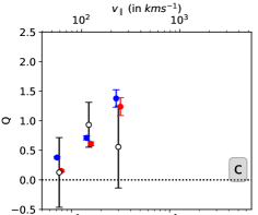
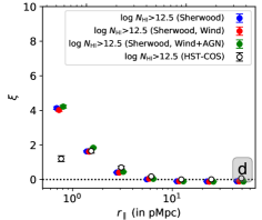
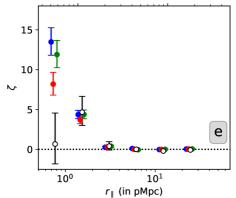
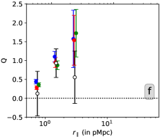
Figure 12: Top panels: Results from MBII simulations. Longitudinal two-point (left), three-point (middle) and reduced three-point (right) correlations of Ly$\alpha$ absorbers as a function of longitudinal scale in simulations for $N_{\rm HI}>10^{12.5}$cm^-2. Results for simulated spectra with two different SNR and including $b_{\rm turb}$ in the case of SNR=50 are presented together with the observations. Bottom panels: Results from all the three simulations in the Sherwood suite studied here.

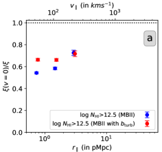
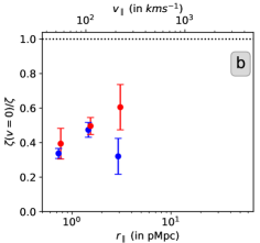
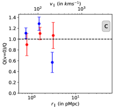
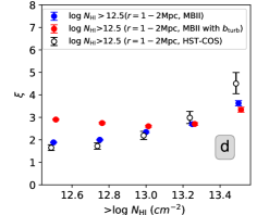
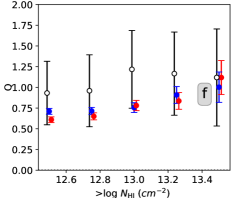
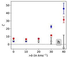
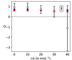
Figure 13: Dependence of redshift space distortions (top panels), $N_{\rm HI}$ thresholds (middle panels) and $b$ thresholds (bottom panels) on the longitudinal two-point (left), three-point (middle) and reduced three-point (right) correlations of Ly$\alpha$ absorbers in MBII simulations. In the top row we show the results as a function of $r_{\parallel}$ for two $N_{\rm HI}$ thresholds. In the bottom two rows we show the results for $r_{\parallel}=1-2$ pMpc, with and without including $b_{\rm turb}$.

In the left, middle and right panels of Fig. 12, we plot two-point, three-point and reduced three-point correlations respectively as a function of $r_{\parallel}$. Results from MBII simulations (with and without $b_{\rm turb}$) and Sherwood simulations are presented in the top and bottom rows respectively. The errors in the correlations are one-sided poissonian uncertainty for the data-data pairs computed over 8000 sightlines in case of the MBII simulation and 4000 sightlines for each of the Sherwood simulations. For both simulations, unlike in observations, there is no suppression of two- or three-point correlation in the first bin (i.e $r_{\parallel}<$ 1 pMpc). In the case of MBII simulations, the predicted two- and three-point functions roughly follow the observations for $r_{\parallel}>1$ pMpc. In the $r_{\parallel}=1-2$ pMpc bin, the two- and three-point correlation are found to be $1.65^{+0.13}_{-0.13}$ and $4.76^{+1.98}_{-1.67}$, respectively. In case of simulations, they are found to be $1.88^{+0.02}_{-0.02}$ and $3.83^{+0.19}_{-0.18}$, respectively. When we include $b_{\rm turb}$, the predicted correlations are higher for $r_{\parallel}<4$ pMpc. As noted in Fig. 10, in these models there is a reduction in the number of low $N_{\rm HI}$  absorbers. Thus we may be probing clustering among the relatively high $N_{\rm HI}$  absorbers even when we use the same $N_{\rm HI}$ cut-off when we include $b_{\rm turb}$. This exercise, clearly illustrates that simple addition of a constant $b_{\rm turb}$ in quadrature to thermal $b$ will not provide correct solution to the missing sub-grid physics.

In the case of Sherwood simulations, the predicted two-point and three-point correlations are also roughly consistent with the observations as well as with the MBII simulation. In the $r_{\parallel}=1-2$ pMpc bin, the two- and three-point correlation are found to be $1.84^{+0.04}_{-0.04}$ and $4.38^{+0.57}_{-0.53}$, respectively for the Wind+AGN case. In the case of two-point correlations, the difference between the predictions of the three Sherwood simulations are small (within $\sim$13%). In the case of three-point correlation the dispersion between the three models is slightly higher ( within $\sim$17%) but still consistent within errors. Therefore, it appears that various feedback process included in the Sherwood simulations produce little difference to the predicted $\xi$ and $\zeta$ at various scales.

In summary, the simulations considered here roughly reproduce the observed profile of $\xi$ and $\zeta$ at scales greater than 1 pMpc . This could just be the mere reflection of the large scale Ly$\alpha$ distribution being consistent with matter distribution in the $\Lambda$CDM models. The difference between the two simulations can come from slightly different cosmological parameters used (see initial paragraphs of section 5 for details). However, the models fail to reproduce the large suppression we notice for $r_{\parallel}<1$ pMpc in the observations. The suppression in the first bin could originate from: (i) difference in the SNR between simulations and observations; (ii) differences in density field at small scales like presence of excess smoothing in the observed data (as suggested by $b$-distribution) and (iii) differences in the line fitting routine used. Note the simulated spectra have higher SNR and typically individual components have lower $b$-values. This helps in the component decomposition of the blended profile and this could provide higher measured correlations at the lowest velocity bin. We confirm that the difference is not due to our automatic Voigt profile routine viper ( which we use for fitting simulated spectra) as our fits to the observational data produce consistent results to what we get from the line list of Danforth et al. (2016) ( which we have used for calculating observed correlations). Our analysis of simulated data with SNR = 12 did not show large suppression in correlation function at $r<1$ pMpc. Therefore, it is possible that the simulations do not capture the density distribution at small scales (i.e missing sub-grid physics). This could also be the reason for the simulated $b$ distribution being different from the observed one as seen in Fig 10.

5.2.1 Reduced three-point correlation function (Q):

Maitra et al. (2020), in their $z\sim 2$ simulations, have found that the reduced three-point correlation function is less sensitive to the astrophysical parameters compared to $\xi$ or $\zeta$. In panels (c) and (f) of Fig. 12, we plot the Q values predicted in simulations as a function of $r_{\parallel}$. In the observations, we do not see any evidence for the scale dependent Q due to large measurement errors. However, it is evident that the simulated Q values increase with increasing scale in the case of MBII simulation. Similar trend is also seen for Sherwood simulations, but with large errorbars. In the case of MBII, Q values tend to be lower in the model with $b_{\rm turb}$ (i.e Q = $0.61^{+0.04}_{-0.04}$) is lower than that without $b_{\rm turb}$ (i.e Q = $0.71^{+0.04}_{-0.04}$) at $r_{\parallel}=1-2$ pMpc bin.

We also notice Q values measured in MBII are slightly lower than what is found in the case of Sherwood simulations (Q for Sherwood simulation having Wind+AGN feedback is $0.88^{+0.12}_{-0.12}$ at $r_{\parallel}=1-2$ pMpc bin). However, thanks to large errors, Q values predicted by different simulations are consistent with observed values ($0.95^{+0.39}_{-0.38}$) at $r_{\parallel}=1-2$ pMpc bin. We need to keep in mind that MBII and Sherwood simulations use slightly different cosmologies (i.e $\Omega_{m}$ and $h$ differ by $\sim$10% and $\sigma_{8}$ is consistent within 2%). We notice that Q also depends on the feedback process included in the simulations (see panel (f) in Fig. 12) . The 80-512 Sherwood simulation produces slightly large Q values compared to those include feedback effects. However, these differences are smaller than the difference in Q we see between different scales in simulations.

5.2.2 Effect of peculiar velocities:

In this section, using MBII simulations, we study the effects of the line of sight peculiar velocities on the measured correlation functions. For this case, we switch off all the peculiar velocities (considering only the cosmological expansion and thermal broadening effects) while generating the mock spectra. We then fit Voigt profiles to these spectra to identify individual components for our clustering analysis. In the top panels of Fig. 13, we present the ratio of measurements without and with the inclusion of line of sight velocity fields for MBII simulations.

The presence of line of sight velocity field is found increase both $\xi$ and $\zeta$ for length scales of our interest. At the scale of 1.0-2.0 pMpc, two-point and three-point correlations are amplified by a factor of $\sim 1.7$ and 2.1, respectively by the line of sight velocity field. This could imply the Ly$\alpha$ absorbers are part of converging flows. On the other hand, presence of line of sight velocity field makes Q weaker at smaller scales ( $r_{\parallel}<2$pMpc). At the scale of 1.0-2.0 pMpc, redshift space distortion reduced the intrinsic Q value by a factor of $\sim 0.3$ ( though with large errorbars). We confirm similar trends in Sherwood simulations also (not shown here). Due to large errors we did not probe the effect of peculiar velocity on Q at large scales (i.e $r>4$ pMpc).

The discussions presented here suggests that the actual matter clustering is smaller (roughly 60% and 50% in the case of two- and three-point correlations, respectively) than what we measure in the redshift space without accounting for the peculiar velocities. The actual Q values are slightly larger at smaller scales. This trend is similar to what is found in the higher order clustering of galaxies. As shown in Fig.4 of McBride et al. (2011a), the projected measurements of Q are found to be slightly larger than the redshift space measurements at smaller scales. At larger scales, they roughly follow each other. Marín et al. (2008) reports similar trends based on the real space vs redshift space distribution of galaxies from cosmological simulations.

5.2.3 Dependence on $N_{\rm HI}$

Next we study the $N_{\rm HI}$ dependence of simulated correlation statistics. In panels d-f in Fig. 13, we plot two-point($\xi$), three-point ($\zeta$) and reduced three-point (Q) correlation functions measured at $r_{\parallel}$ = 1-2 pMpc as a function of $N_{\rm HI}$ thresholds. In panel (d) and (e), we find that the two- and three-point correlations steadily increases with increasing $N_{\rm HI}$ threshold. While the trend seen is similar to what we see in observations we see the increase in $\xi$ and $\zeta$ with $N_{\rm HI}$ threshold is slightly slower as compared to what is seen in the case of observations. This could be related to the lack of high $N_{\rm HI}$ absorbers in simulations compared to observed distribution.

The measured $\xi$ and $\zeta$ values for low $N_{\rm HI}$ threshold are higher when we include $b_{\rm turb}$. However, the results are consistent for higher $N_{\rm HI}$ thresholds for models with and without $b_{\rm turb}$ included. As discussed before inclusion of $b_{\rm turb}$ reduces the number of low $N_{\rm HI}$ systems detected, which cluster weakly. Therefore, for low $N_{\rm HI}$ thresholds we get enhancement in $\xi$ and $\zeta$. However, $N_{\rm HI}$ distribution is not affected at high $N_{\rm HI}$ thresholds by $b_{\rm turb}$ (see Fig 10). Therefore, $\xi$ and $\zeta$ values are similar at high $N_{\rm HI}$ thresholds. This also suggests that fixing the shortcomings of the simulation (i.e sub-grid physics) using a constant $b_{\rm turb}$ term is not the correct solution.

The dependence of Q on $N_{\rm HI}$ threshold is shown in panel (f) of Fig. 13. The Q remains nearly constant and consistent value with observations. As expected the inclusion of $b_{\rm turb}$ reduces the Q values in the low $N_{\rm HI}$ range.

5.2.4 Dependence on $b$-parameter

In observations, we found the two- and three-point correlation function is independent of $b$-threshold for low threshold values (see Fig. 3). We did find the suppression when we consider systems with $b>40$ $kms^{-1}$(i.e high-$b$ absorbers). When we consider high- and low-$b$ sub-samples (see Fig. 6) three-point correlation was not detected in the case of high-$b$ sub-sample. In panels (g)-(i) in Fig. 13, we plot two-point, three-point and reduced three-point correlation functions at a scale of 1-2 pMpc as a function of $b$ thresholds. We show the results from MBII simulations with and without addition of $b_{\rm turb}$. It is evident from this figure that unlike observations both two- and three-point correlation functions show monotonic increasing with increasing $b$-threshold even for the high-$b$ absorbers. We also notice that Q has very weak dependence on $b$ threshold.

When we include $b_{\rm turb}$ as expected the $\xi$ and $\zeta$ are independent of limiting $b$ when it is less than 20 $kms^{-1}$. However shows monotonous increase with increasing $b$ afterwards. In particular detection of positive $\zeta$ for $b>40$ $kms^{-1}$ is intriguing. We believe the difference is dominated by two possible effects (i) higher SNR used in our simulations and (ii) the differences in the $b$-distribution between simulations and observations noted before. That is a given b-threshold will pick typically high $N_{\rm HI}$ systems in the simulations compared to observation (see Fig 11).

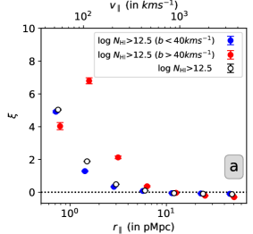
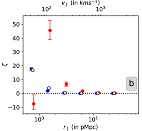
Figure 14: Two-point (panel a) and three-point (panel b) correlations of Ly$\alpha$ absorbers in MBII simulation for full sample, high-$b$ ($b>40$ $kms^{-1}$) and low-$b$ ($b<$ 40 $kms^{-1}$) sub-samples. Unlike in the case of observations (see Fig. 6) high-$b$ absorbers show stronger two- and three-point correlations at large scales.

To investigate this further in Fig 14, we plot the radial dependence of two- and three-point correlation functions for low- and high-$b$ sub-samples from our simulations (similar to Fig 6 for observations). For $r>1$ pMpc, two and three-point correlation function of high-$b$ systems are found to be larger than those of low-$b$ systems. We notice that when we consider SNR = 12 simulations, as in observations we do not detect positive three point correlations for $r<4$ pMpc. However we notice that these models have much larger two-point correlation at r = 1-2 pMpc bin. Therefore we conclude that while low SNR in the observations have a role to play in suppressing the three-point correlation in the case of high-$b$ absorbers this alone can not explain the increase in $\xi$ and $\zeta$ we find as a function of $b$-threshold.

6 Main results & discussions:

We report the detection of longitudinal (redshift space) three-point correlation function ($\zeta$) of $z\leq 0.48$ Ly$\alpha$ absorbers using HST-COS spectra of 82 QSOs compiled by Danforth et al. (2016). We study the dependence of $\zeta$ on $N_{\rm HI}$, $b$-parameter, $z$ and presence of metals. We also correlate the Ly$\alpha$ absorbers at $z<0.2$ contributing to the three-point correlation function with the galaxy distribution for 41 of these sightlines. We compute Ly$\alpha$ clustering using four different simulation boxes at $z\sim 0.1$ and compare them with observations. Here we discuss the main results of our study.

Clustering properties of low-z IGM: Danforth et al. (2016) has shown that the low-$z$ Ly$\alpha$ absorbers cluster among themselves up to a scale of $\sim$10 pMpc with a positive two-point correlation. Using the same data, we report for the first time the detection of a non-zero probability excess in Ly$\alpha$ triplets ($\rm PE_{3}$) up to 8 pMpc, with the strongest detection ($\rm PE_{3}=8.8^{+2.0}_{-1.7}$ for absorbers having $N_{\rm HI}$$\geq 10^{12.5}$ cm^-2) coming from the $r_{\parallel}=1-2$ pMpc bin with equal arm configuration at a significance level of $\sim 5\sigma$. In the case of 1:2 arm ratio configuration, we find $\rm PE_{3}=2.1^{+0.5}_{-0.4}$ (4$\sigma$ level) for $r_{\parallel,1}=1-2$ pMpc and $r_{\parallel,2}=2-4$ pMpc. Using the triplet probability excess we obtain positive longitudinal three-point correlation ($\zeta$) at scales below 4 pMpc. The strongest detection is at the scale of 1-2 pMpc with equal arm configuration ($\zeta=4.8^{+2.0}_{-1.7}$) for $N_{\rm HI}$$\geq 10^{12.5}$ cm^-2). These are the first reported measurements of three-point correlation function from the Ly$\alpha$ forest observations and using Voigt profile decomposed components. We do not detect any three-point correlation for 1:2 arm ratio configurations. The measured amplitudes of Ly$\alpha$ three-point correlation is at least an order of magnitude weaker than that measured for galaxies ($\zeta\sim 200$ for $M_{r}<-19$ galaxies at $r\sim 1$ pMpc and $\theta=0$ for $r_{1}:r_{2}=1:2$ configuration; see Guo et al. (2016)). Using our measured $\xi$ and $\zeta$ we obtain the reduced three-point correlation function Q ($0.95^{+0.39}_{-0.38}$) for $r_{\parallel}=1-2$ pMpc bin and equal arm configuration . This is similar to the Q values measured in the case of low-$z$ galaxies (see figure 4 of McBride et al., 2011a, for $\theta=0$ for $r_{1}:r_{2}=1:2$ configurations).

Both two- and three-point correlations are suppressed for $r_{\parallel}<$ 1.0 pMpc (or $r_{\parallel}<$72$kms^{-1}$ at $z\sim 0.1$). This suppression is related to the efficiency at which Voigt profile decomposition can be performed at these scales. This depends on the matter distribution at small scales, instrumental resolution, line blending, SNR of the spectra used (see Danforth et al., 2016). Measuring $\zeta$ and $\xi$ in the transverse direction using closely spaced quasar sightlines will be important to have further insights into this issue.

For $r_{\parallel}>1$ pMpc, both two- and three-point correlations show a decreasing trend with increasing scale. However, we do not notice any scale dependence of Q for $r_{\parallel}>1$ pMpc range in the observations, thanks to large measurement errors. In the case of galaxies Q values are measured over much larger scales (i.e 3-20 pMpc) and found to be scale independent when peculiar velocity effects are taken care of (McBride et al., 2011b).

Dependence of $N_{\rm HI}$: As we discussed in the introduction, it is known that the $N_{\rm HI}$ of an absorption feature is related to the underlying baryonic (and dark matter) overdensities. At low-$z$, it is also known that high $N_{\rm HI}$ systems ($N_{\rm HI}>10^{14}$cm^-2) strongly cluster around galaxies while the weaker absorbers are distributed more randomly or associated with low density IGM or galaxy voids (Penton et al., 2002; Tejos et al., 2014). It is also known that the stronger $N_{\rm HI}$ absorbers have larger two-point correlation compared to low $N_{\rm HI}$ absorbers (see Penton et al., 2002; Danforth et al., 2016, for example). In this work, we find that like two-point correlation the three-point correlation function of the Ly$\alpha$ absorbers also shows an increasing tendency with increasing $N_{\rm HI}$ thresholds for a given scale probed. Compared to $\zeta=4.8^{+2.0}_{-1.7}$ for $N_{\rm HI}>10^{12.5}$cm^-2 absorbers, we obtain $\zeta=34.2^{+19.4}_{-14.1}$ for $N_{\rm HI}>10^{13.5}$cm^-2 absorbers. On the other hand, the reduced three-point correlation Q is relatively independent of the $N_{\rm HI}$ thresholds.

Dependence on b-parameter: While the low-$b$ Ly$\alpha$ absorbers ($b<40$ $kms^{-1}$) probe the cool photoionized gas, some fraction of the high-$b$ Ly$\alpha$ absorbers ($b>40$ $kms^{-1}$) could arise from the highly ionized warm hot intergalactic gas or WHIM (Richter et al., 2006; Tepper-García et al., 2012). Atleast 20% of the total baryonic content of the Universe is located in highly ionized WHIM and the cool photoionized gas comprises of about 30% of the baryons (Lehner et al., 2007). A $b$-dependent clustering study essentially allows us to probe matter distribution as one transitions from one gaseous phase to another. We find the two-point correlation (probed over 1-2 pMpc) to remain nearly constant for low-$b$ thresholds but shows a decreasing trend when we consider absorbers with $b>40$ $kms^{-1}$. This trend is also seen in the case of three-point correlation albeit with a much sharper decrease. When we consider high- and low-$b$ sub-samples based on $b$-parameter the measured radial profiles of two- and three-point correlations are found to be very different. While low-$b$ sub-sample shows positive three-point correlation for $r_{\parallel}<$ 4 pMpc no correlation is detected for high-$b$ sub-sample over the same scale. The lack of three-point correlation among high-$b$ systems could be related to biases involved in detected three such absorbers in smaller velocity separations using automatic Voigt profile fits. Therefore, to draw any useful physical conclusions it will be important to confirm this result with high SNR data. Just to quantify this, we considered the number of high-b ($b>40$ $kms^{-1}$) triplets seen in 8000 sightlines (i.e $dz\sim 290$ which is $\sim$ 15 times the redshift path of the observed sample used here) of simulated data for two SNR values (i.e 12 and 50). In the case of SNR of 50, we identify 4 and 88 high-b triplets in the first two r bins (i.e 0.5-1.0 and 1.0-2.0 pMpc). However, for SNR of 12, we do not find any triplet. This clearly demonstrates that, while having a larger path length is always useful for detecting the signal at a higher significant level, better SNR is crucial for the identification of the high-$b$ triplets.

Metal components and clustering: Danforth et al. (2016) have shown that metal bearing Ly$\alpha$ absorbers cluster strongly compared to those without detectable metals. Therefore, we investigated whether the three-point correlation we see comes mainly from these metal bearing Ly$\alpha$ components. For this we identified Ly$\alpha$ absorption with associated C iv, O vi and Si iii absorption (with rest equivalent width more than 30 mÅ). We studied the Ly$\alpha$ clustering excluding these components with metal detection. This exercise confirmed that our clustering measurements are not dominated by the metal bearing Ly$\alpha$ absorbers. As metal line systems are sparse it is not possible to probe the three-point correlation between these systems using the present data.

Connection to Galaxy distribution: Since the distance scale probed in our study corresponds to velocity ranges consistent with what one expects in galaxy halos it is also important to see the contribution of CGM absorption to the measured clustering. We use the catalog of $z<0.2$ galaxies around the 41 quasars available in the literature (Keeney et al., 2018; Prochaska et al., 2011) to study the relationship between Ly$\alpha$ triplets and galaxy distribution. We find majority of Ly$\alpha$ triplet systems at $z<0.2$ to have nearby galaxies. For the chosen triplet configurations ($r_{1}=r_{2}=0.5-1$ pMpc, $1-2$ pMpc, $2-4$ pMpc and $r_{1}=0.5-1$ pMpc, $r_{2}=1-2$ pMpc), we find that 88% of the triplets have at least one nearby galaxy within a velocity separation of 500 $kms^{-1}$. The impact parameters of these galaxies range from 62-3854 pkpc (median of 405 pkpc). Therefore, a good fraction of triplets originate from impact parameters that are inconsistent with them being associated to a single galaxy. We also find that the impact parameters of isolated Ly$\alpha$ absorption is statistically larger than that of the doublets and triplets. This suggest that multiple component Ly$\alpha$ absorbers are more closely related to galaxies than the isolated absorbers. All these are consistent with the clustered Ly$\alpha$ regions being closer to the galaxy distributions. We also find that $b>40$ $kms^{-1}$BLA absorbers occur more frequently for triplet systems ($\sim 85$%) in comparison to individual absorbers ($\sim 31.9$%) . As we mentioned before, Wakker et al. (2015) found that the Ly$\alpha$ absorption with $N_{\rm HI}$$\geq 10^{13}$ cm^-2 have the filament impact parameter less than 2.1 pMpc and all BLAs are found to be located within 400 pkpc to the filament axis and all the absorbers showing multiple velocity components are located within 1 pMpc to the filament axis. Tejos et al. (2016) have also found the BLAs have high detection rate close to the filament connecting cluster pairs in the redshift range $0.1<z<0.5$. Thus our results are consistent with clustered regions originating from filament like structures. Establishing such a connection will allow us to interpret the redshift evolution of $\zeta$ in terms of evolution on large scale structures. However, we need more sensitive galaxy observations over a wider projected scale compared to what has been used in this study.

Clustering in the simulated data: The four different hydrodynamical simulations considered here roughly reproduce the scale dependence of of $\xi$, $\zeta$ and Q for $r_{\parallel}>1$ pMpc (within 2$\sigma$ level). This is could just be the reflection of matter distribution at large scale being consistent with $\Lambda$CDM predictions. At the smallest scale, the simulations (performed at SNR $\sim$ 50) do not show suppression as seen in the data. The simulations also show a similar dependence of $\xi$, $\zeta$ and Q on $N_{\rm HI}$ as the observations. However, the rate of increase of $\zeta$ and $\xi$ with $N_{\rm HI}$ is found to be lower in simulations. We also note that different feedback processes have little effect on the observed clustering. Unlike observations, simulations show a monotonic increase in $\zeta$ and $\xi$ with $b$-parameter. This differences could be linked to the fact that none of the simulations correctly reproduce the observed distribution of $b$-parameter and $N_{\rm HI}$ distribution at high $N_{\rm HI}$ range. While low SNR of the observed data may explain lack of three-point correlation among high-$b$ systems, this alone can not explain the $b$-dependent trend found in observations.

Using our simulations we find that the line of sight peculiar velocities tend to amplify the observed $\xi$ and $\zeta$ by a factor of $\sim$ 1.7 and 2.1, respectively, compared to the real space clustering. The effect on Q value is smaller. The Q values are seemingly suppressed by $\sim$30% within $r_{\parallel}=2$pMpc with large errorbars. This is similar to the findings in McBride et al. (2011a) for clustering of SDSS galaxies, wherein the projected measurements of Q are found to be slightly larger than the redshift space measurements at smaller scales. Similar results are also reported based on galaxy distribution in real space vs redshift space from cosmological simulations in Marín et al. (2008).

Future directions: It is important to accurately measure the three point correlation and Q preferable over larger scales. This will allow us to measure the linear and non-linear bias parameter for the Ly$\alpha$ forest. With the existing archival data it is possible to improve our measurement by more than 50%. The scale dependence of Q (shown by simulations) is interesting. As we discussed in the introduction, low-$z$ Ly$\alpha$ may originate from CGM, ICM, IGM or from the interface region between them. If different populations trace different scales that can lead to a scale dependent Q values. Non-linear clustering studies also predict scale dependent Q values. Accurate measurement of $Q$ over different scales is therefore very important.

In the simulation front, it is important to have large simulations with appropriate sub-grid physics to first match the observed $N_{\rm HI}$ and $b$-distributions before trying to match the observed clustering properties of the Ly$\alpha$ absorbers. It is also important to calibrate the simulations to correctly produce the properties of metal line absorbers to be able to probe the influence of feedback on the clustering properties of low-$z$ absorbers. Such a constrained simulation will allow us to establish a connection between large scale structure and the Ly$\alpha$ absorbers.

Data Availability

HST-COS data products of Danforth et al. (2016) used in this study can be accessed from https://archive.stsci.edu/prepds/igm/.

References

- Aracil et al. (2002) Aracil B., Petitjean P., Smette A., Surdej J., Mücket J. P., Cristiani S., 2002, A&A, 391, 1
- Bahcall et al. (1991) Bahcall J. N., Jannuzi B. T., Schneider D. P., Hartig G. F., Bohlin R., Junkkarinen V., 1991, ApJ, 377, L5
- Bahcall et al. (1993) Bahcall J. N., et al., 1993, ApJS, 87, 1
- Bahcall et al. (1996) Bahcall J. N., et al., 1996, ApJ, 457, 19
- Bernardeau et al. (2002) Bernardeau F., Colombi S., Gaztañaga E., Scoccimarro R., 2002, Phys. Rep., 367, 1
- Bi & Davidsen (1997) Bi H., Davidsen A. F., 1997, ApJ, 479, 523
- Bolton et al. (2017) Bolton J. S., Puchwein E., Sijacki D., Haehnelt M. G., Kim T.-S., Meiksin A., Regan J. A., Viel M., 2017, MNRAS, 464, 897
- Burchett et al. (2018) Burchett J. N., Tripp T. M., Wang Q. D., Willmer C. N. A., Bowen D. V., Jenkins E. B., 2018, MNRAS, 475, 2067
- Cappetta et al. (2010) Cappetta M., D’Odorico V., Cristiani S., Saitta F., Viel M., 2010, MNRAS, 407, 1290
- Coppolani et al. (2006) Coppolani F., et al., 2006, MNRAS, 370, 1804
- Croft et al. (2002) Croft R. A. C., Weinberg D. H., Bolte M., Burles S., Hernquist L., Katz N., Kirkman D., Tytler D., 2002, ApJ, 581, 20
- D’Odorico et al. (2006) D’Odorico V., et al., 2006, MNRAS, 372, 1333
- Danforth & Shull (2008) Danforth C. W., Shull J. M., 2008, ApJ, 679, 194
- Danforth et al. (2016) Danforth C. W., et al., 2016, ApJ, 817, 111
- Davé et al. (2001) Davé R., et al., 2001, ApJ, 552, 473
- Davé et al. (2010) Davé R., Oppenheimer B. D., Katz N., Kollmeier J. A., Weinberg D. H., 2010, MNRAS, 408, 2051
- Fry (1994) Fry J. N., 1994, Phys. Rev. Lett., 73, 215
- Gaikwad et al. (2017a) Gaikwad P., Khaire V., Choudhury T. R., Srianand R., 2017a, MNRAS, 466, 838
- Gaikwad et al. (2017b) Gaikwad P., Srianand R., Choudhury T. R., Khaire V., 2017b, MNRAS, 467, 3172
- Gaikwad et al. (2019) Gaikwad P., Srianand R., Khaire V., Choudhury T. R., 2019, MNRAS, 490, 1588
- Gaikwad et al. (2020a) Gaikwad P., Srianand R., Haehnelt M. G., Choudhury T. R., 2020a, arXiv e-prints, p. arXiv:2009.00016
- Gaikwad et al. (2020b) Gaikwad P., et al., 2020b, MNRAS, 494, 5091
- Groth & Peebles (1977) Groth E. J., Peebles P. J. E., 1977, ApJ, 217, 385
- Guo et al. (2016) Guo H., et al., 2016, The Astrophysical Journal, 831, 3
- Gurvich et al. (2017) Gurvich A., Burkhart B., Bird S., 2017, ApJ, 835, 175
- Haardt & Madau (1996) Haardt F., Madau P., 1996, ApJ, 461, 20
- Haardt & Madau (2012) Haardt F., Madau P., 2012, ApJ, 746, 125
- Hennawi et al. (2010) Hennawi J. F., et al., 2010, ApJ, 719, 1672
- Hussain et al. (2017) Hussain T., Khaire V., Srianand R., Muzahid S., Pathak A., 2017, MNRAS, 466, 3133
- Impey et al. (1999) Impey C. D., Petry C. E., Flint K. P., 1999, ApJ, 524, 536
- Keeney et al. (2018) Keeney B. A., et al., 2018, ApJS, 237, 11
- Kerscher et al. (2000) Kerscher M., Szapudi I., Szalay A. S., 2000, ApJ, 535, L13
- Khaire & Srianand (2015) Khaire V., Srianand R., 2015, MNRAS, 451, L30
- Khaire & Srianand (2019) Khaire V., Srianand R., 2019, MNRAS, 484, 4174
- Khaire et al. (2019) Khaire V., et al., 2019, MNRAS, 486, 769
- Khandai et al. (2015) Khandai N., Di Matteo T., Croft R., Wilkins S., Feng Y., Tucker E., DeGraf C., Liu M.-S., 2015, MNRAS, 450, 1349
- Kollmeier et al. (2014) Kollmeier J. A., et al., 2014, ApJ, 789, L32
- Komatsu et al. (2011) Komatsu E., et al., 2011, ApJS, 192, 18
- Lehner et al. (2007) Lehner N., Savage B. D., Richter P., Sembach K. R., Tripp T. M., Wakker B. P., 2007, ApJ, 658, 680
- Maitra et al. (2019) Maitra S., Srianand R., Petitjean P., Rahmani H., Gaikwad P., Choudhury T. R., Pichon C., 2019, MNRAS, 490, 3633
- Maitra et al. (2020) Maitra S., Srianand R., Gaikwad P., Choudhury T. R., Paranjape A., Petitjean P., 2020, MNRAS, 498, 6100
- Marín et al. (2008) Marín F. A., Wechsler R. H., Frieman J. A., Nichol R. C., 2008, ApJ, 672, 849
- McBride et al. (2011a) McBride C. K., Connolly A. J., Gardner J. P., Scranton R., Newman J. A., Scoccimarro R., Zehavi I., Schneider D. P., 2011a, The Astrophysical Journal, 726, 13
- McBride et al. (2011b) McBride C. K., Connolly A. J., Gardner J. P., Scranton R., Scoccimarro R., Berlind A. A., Marín F., Schneider D. P., 2011b, The Astrophysical Journal, 739, 85
- McDonald et al. (2000) McDonald P., Miralda-Escudé J., Rauch M., Sargent W. L. W., Barlow T. A., Cen R., Ostriker J. P., 2000, ApJ, 543, 1
- McDonald et al. (2005) McDonald P., et al., 2005, ApJ, 635, 761
- McDonald et al. (2006) McDonald P., et al., 2006, ApJS, 163, 80
- Meiksin (2009) Meiksin A. A., 2009, Reviews of Modern Physics, 81, 1405
- Muzahid et al. (2017) Muzahid S., Charlton J., Nagai D., Schaye J., Srianand R., 2017, ApJ, 846, L8
- Narayanan et al. (2000) Narayanan V. K., Spergel D. N., Davé R., Ma C.-P., 2000, ApJ, 543, L103
- Nasir et al. (2017) Nasir F., Bolton J. S., Viel M., Kim T.-S., Haehnelt M. G., Puchwein E., Sijacki D., 2017, MNRAS, 471, 1056
- Oppenheimer & Davé (2009) Oppenheimer B. D., Davé R., 2009, MNRAS, 395, 1875
- Palanque-Delabrouille et al. (2013) Palanque-Delabrouille N., et al., 2013, A&A, 559, A85
- Palanque-Delabrouille et al. (2015a) Palanque-Delabrouille N., et al., 2015a, J. Cosmology Astropart. Phys., 2, 045
- Palanque-Delabrouille et al. (2015b) Palanque-Delabrouille N., et al., 2015b, J. Cosmology Astropart. Phys., 11, 011
- Palanque-Delabrouille et al. (2020) Palanque-Delabrouille N., Yèche C., Schöneberg N., Lesgourgues J., Walther M., Chabanier S., Armengaud E., 2020, J. Cosmology Astropart. Phys., 2020, 038
- Peebles (1980) Peebles P. J. E., 1980, The large-scale structure of the universe
- Peebles & Groth (1975) Peebles P. J. E., Groth E. J., 1975, ApJ, 196, 1
- Peeples et al. (2010a) Peeples M. S., Weinberg D. H., Davé R., Fardal M. A., Katz N., 2010a, MNRAS, 404, 1281
- Peeples et al. (2010b) Peeples M. S., Weinberg D. H., Davé R., Fardal M. A., Katz N., 2010b, MNRAS, 404, 1295
- Penton et al. (2000) Penton S. V., Shull J. M., Stocke J. T., 2000, ApJ, 544, 150
- Penton et al. (2002) Penton S. V., Stocke J. T., Shull J. M., 2002, ApJ, 565, 720
- Petitjean et al. (1993) Petitjean P., Webb J. K., Rauch M., Carswell R. F., Lanzetta K., 1993, MNRAS, 262, 499
- Petitjean et al. (1998) Petitjean P., Surdej J., Smette A., Shaver P., Muecket J., Remy M., 1998, A&A, 334, L45
- Pierleoni et al. (2008) Pierleoni M., Branchini E., Viel M., 2008, MNRAS, 388, 282
- Planck Collaboration et al. (2014) Planck Collaboration et al., 2014, A&A, 571, A16
- Prochaska et al. (2011) Prochaska J. X., Weiner B., Chen H. W., Cooksey K. L., Mulchaey J. S., 2011, ApJS, 193, 28
- Puchwein & Springel (2013) Puchwein E., Springel V., 2013, MNRAS, 428, 2966
- Rauch (1998) Rauch M., 1998, ARA&A, 36, 267
- Rauch & Haehnelt (1995) Rauch M., Haehnelt M. G., 1995, MNRAS, 275, L76
- Richter et al. (2006) Richter P., Savage B. D., Sembach K. R., Tripp T. M., 2006, A&A, 445, 827
- Rollinde et al. (2013) Rollinde E., Theuns T., Schaye J., Pâris I., Petitjean P., 2013, MNRAS, 428, 540
- Rudie et al. (2012) Rudie G. C., et al., 2012, ApJ, 750, 67
- Savage et al. (2005) Savage B. D., Lehner N., Wakker B. P., Sembach K. R., Tripp T. M., 2005, ApJ, 626, 776
- Seljak et al. (2006) Seljak U., Slosar A., McDonald P., 2006, J. Cosmology Astropart. Phys., 10, 014
- Shull et al. (2015) Shull J. M., Moloney J., Danforth C. W., Tilton E. M., 2015, ApJ, 811, 3
- Smette et al. (1995) Smette A., Robertson J. G., Shaver P. A., Reimers D., Wisotzki L., Koehler T., 1995, A&AS, 113, 199
- Smith et al. (2011) Smith B. D., Hallman E. J., Shull J. M., O’Shea B. W., 2011, ApJ, 731, 6
- Springel (2005) Springel V., 2005, MNRAS, 364, 1105
- Stocke et al. (1995) Stocke J. T., Shull J. M., Penton S., Donahue M., Carilli C., 1995, ApJ, 451, 24
- Stocke et al. (2013) Stocke J. T., Keeney B. A., Danforth C. W., Shull J. M., Froning C. S., Green J. C., Penton S. V., Savage B. D., 2013, ApJ, 763, 148
- Tejos et al. (2014) Tejos N., et al., 2014, MNRAS, 437, 2017
- Tejos et al. (2016) Tejos N., et al., 2016, MNRAS, 455, 2662
- Tepper-García et al. (2012) Tepper-García T., Richter P., Schaye J., Booth C. M., Dalla Vecchia C., Theuns T., 2012, MNRAS, 425, 1640
- Tie et al. (2019) Tie S. S., Weinberg D. H., Martini P., Zhu W., Peirani S., Suarez T., Colombi S., 2019, MNRAS, 487, 5346
- Tilton et al. (2016) Tilton E. M., Stevans M. L., Shull J. M., Danforth C. W., 2016, ApJ, 817, 56
- Tripp et al. (2008) Tripp T. M., Sembach K. R., Bowen D. V., Savage B. D., Jenkins E. B., Lehner N., Richter P., 2008, ApJS, 177, 39
- Ulmer (1996) Ulmer A., 1996, ApJ, 473, 110
- Verde et al. (2002) Verde L., et al., 2002, MNRAS, 335, 432
- Viel et al. (2004) Viel M., Matarrese S., Heavens A., Haehnelt M. G., Kim T. S., Springel V., Hernquist L., 2004, MNRAS, 347, L26
- Viel et al. (2005) Viel M., Lesgourgues J., Haehnelt M. G., Matarrese S., Riotto A., 2005, Phys. Rev. D, 71, 063534
- Viel et al. (2013) Viel M., Becker G. D., Bolton J. S., Haehnelt M. G., 2013, Phys. Rev. D, 88, 043502
- Viel et al. (2017) Viel M., Haehnelt M. G., Bolton J. S., Kim T.-S., Puchwein E., Nasir F., Wakker B. P., 2017, MNRAS, 467, L86
- Wakker et al. (2015) Wakker B. P., Hernandez A. K., French D. M., Kim T.-S., Oppenheimer B. D., Savage B. D., 2015, ApJ, 814, 40
- Walther et al. (2019) Walther M., Oñorbe J., Hennawi J. F., Lukić Z., 2019, ApJ, 872, 13
- Werk et al. (2014) Werk J. K., et al., 2014, ApJ, 792, 8
- Yèche et al. (2017) Yèche C., Palanque-Delabrouille N., Baur J., du Mas des Bourboux H., 2017, J. Cosmology Astropart. Phys., 6, 047