Abstract

In this article, we study the two body gluino decays $\tilde{g}\rightarrow\tilde{u}_{i}\bar{u}_{g}$, $\tilde{g}\rightarrow\tilde{d}_{i}\bar{d}_{g}$ with $i=1,2,...6$ and $g=1,2,3$ in the Minimal Supersymmetric Standard Model (MSSM) with quark flavour violation (QFV). At the outset, constraints on QFV parameters $\delta_{ij}^{U/D(LR)}$ and $\delta_{ij}^{U/D(RL)}$ with $i,j=1,2,3$ and $(i\neq j)$ are calculated for a specific set of MSSM parameters using charge and color breaking minima (CCB) and unbounded from below minima (UFB) conditions. These constraints are more stringent compared to the constraints coming from B-physics observables (BPO), that are already available in literature. In the second step, we re-calculate the partial decay widths of $\tilde{g}\rightarrow\tilde{u}_{i}\bar{u}_{g}$, $\tilde{g}\rightarrow\tilde{d}_{i}\bar{d}_{g}$ for the allowed range of QFV parameters. The partial decay widths can reach upto 120 GeV in the RR sector of the squarks mass matrices while in the LL sector it can be $\approx 90\,\,\mathrm{GeV}$. The QFV in the LR/RL sector is usually ignored due to stringent CCB and UFB constraints. However, our analysis reveals that this mixing can contribute upto $\approx 12\,\,\mathrm{GeV}$ for some parameter points and should not be ignored. We hope that these results will prove helpful for the experimental searches of gluinos at the current and future colliders.

1 Introduction

Minimal Supersymmetric Standard Model (MSSM) [1, 2, 3] is a rather enthralling theory Beyond the Standard Model (SM)[4, 5, 6]. It is able to answer many of the queries that remained unanswered in SM. Search for the supersymmetric particles is one of the major tasks at the large hadron collider experiment at CERN. Therefore, a lot of attention has been devoted to the study of sparticle decays. Gluino decays are particularly interesting as the bounds on the gluino mass are progressively increasing[7]. Analyses of these decays provide the new techniques for experimental searches and deep insight of couplings between standard particles and their super-partners.

Contrary to SM, where CKM matrix is the only source of quark flavour violation (QFV), MSSM contains extra sources [8, 9, 10], in the form of quark-squarks misalignments which appear as the non-diagonal entries in the squarks mass matrices and is parametrized in terms of flavor violating (FV) deltas $\delta_{ij}^{FAB}$, where $i\neq j$ $(i,j=1,2,3)$ and $F=Q,U,D;$ $A,B=L,R$. These FV deltas can result in the large amplitudes for flavour changing neutral current (FCNC) processes. Therefore, there are stringent constraints on these deltas due to FCNC processes. It has been shown in some recent studies [11, 12] that the flavor violating deltas may result in interesting phenomenological effects, contrary to the some previous studies where these deltas were put to zero by hand.

As has already been scientifically broadcasted, the FV delta can also impact the gluino decays. For example gluino decays into quark and squark at tree (with QFV) as well as at loop (without QFV) level were analysed in [13, 14, 15, 16, 17, 18, 19]. Furthermore, QFV gluino decays into a quark and squark at one loop level (mainly focused on $RR$ mixing) were investigated in [20] considering the strong suppression of the $LL$, $LR$ and $RL$ mixings due to FCNC, charge and color breaking minima (CCB) and unbounded from below minima (UFB) [21].

We have extended this analysis by incorporating the contribution of LL, LR and RL mixing in two body gluino decays. As mentioned earlier, the indirect bounds on $\delta_{ij}^{QAB}$ coming from FCNC processes are very strong. First and second generation mixing is severely constrained by $K$-Physics. However, there is some room for the second and third generation mixing. The constraints on $\delta_{23}^{QAB}$ mainly come from B-Physics Observables (BPO). These constraints for a specific set of parameters were calculated in [22]. Using the same set of parameters (with a slight modification of $M_{A}$ value), we have extended their analysis and calculated the CCB and UFB bounds on these deltas. The vacuum stability (CCB and UFB) conditions turned out to be more constraining in the $LR,$ $RL$ sector compared to the constraints from BPO. As a final step, we have analyzed the two body gluino decay using these deltas. For numerical analysis, we have used FeynArts/FormCalc setup [23, 24].

The paper is organized as follows: in Sect. 2 we discuss the salient features of the MSSM and set the notation. Sect. 3 is dedicated to the analytical calculation of gluino decay and some details of BPO, CCB and UFB. In Sect. 4 we discuss our numerical analysis followed by the conclusions of this work in Sect. 5.

2 Model set-up

The R-parity conserving superpotential $W$ of MSSM is given as [1, 2, 3]

$$W=\epsilon_{\alpha\beta}\left[(\lambda_{l})_{ij}\hat{H}_{1}^{\alpha}\hat{L}_{\iota}^{\beta}\hat{E}_{j}^{C}+(\lambda_{d})_{ij}\hat{H}_{1}^{\alpha}\hat{Q}_{\iota}^{\beta}\hat{D}_{j}^{C}+(\lambda_{u})_{ij}\hat{H}_{2}^{\alpha}\hat{Q}_{\iota}^{\beta}\hat{U}_{j}^{C}-\mu\hat{H}_{1}^{\alpha}\hat{H}_{2}^{\beta}\right]$$

where $\lambda$ represents the Yukawa couplings and $\mu$ is the Higgs mass parameter. $\hat{Q}$ is for left-handed quark and squark doublet, $\hat{U}$ is for right-handed up-type quark and squark singlet, and $\hat{D}$ is for right-handed down–type quark and squark singlet. For leptonic fields, there are $\hat{L}$ for left-handed lepton and slepton doublet and $\hat{E}$ for right handed lepton and slepton singlet. There are no right handed neutrinos present in MSSM. $\hat{H}_{1}$ and $\hat{H}_{2}$ are the 2 Higgs superfields. As SUSY is not exact symmetry therefore we have to incorporate SUSY breaking in the MSSM. Accordingly, the soft-SUSY-Breaking Lagrangian can be written as:

$$-\mathcal{L}_{soft} =(m_{\tilde{Q}}^{2})_{i}^{j}\tilde{Q}^{\dagger\iota}\tilde{Q}_{j}+(m_{\tilde{U}}^{2})_{j}^{i}\tilde{U}_{i}^{\ast}\tilde{U}^{j}+(m_{\tilde{D}}^{2})_{j}^{i}\tilde{D}_{i}^{\ast}\tilde{D}^{j}+(m_{\tilde{L}}^{2})_{i}^{j}\tilde{L}^{\dagger\iota}\tilde{L}_{j}$$

$$+(m_{\tilde{E}}^{2})_{j}^{i}\tilde{E}_{\iota}^{\ast}\tilde{E}^{j}+m_{H_{1}}^{2}\hat{H}_{1}^{\dagger}\hat{H}_{1}+m_{H_{2}}^{2}\hat{H}_{2}^{\dagger}\hat{H}_{2}+\left(B\mu\hat{H}_{1}^{\dagger}\hat{H}_{2}+h.c\right)$$

$$+(({\cal A}^{d})_{ij}\hat{H}_{1}\tilde{D}_{i}^{\ast}\tilde{Q}_{j}+({\cal A}^{u})_{ij}\hat{H}_{2}\tilde{U}_{i}^{\ast}\tilde{Q}_{j}+({\cal A}^{l})_{ij}\hat{H}_{1}\tilde{E}_{\iota}^{\ast}\tilde{E}_{j}$$

$$+\frac{1}{2}M_{1}\tilde{B}_{L}^{0}\tilde{B}_{L}^{0}+\frac{1}{2}M_{2}\tilde{W}_{L}^{a}\tilde{W}_{L}^{a}+\frac{1}{2}M_{3}\tilde{G}^{a}\tilde{G}^{a}+h.c)$$ (1)

$m_{\hat{Q}}^{2},$ $m_{\hat{U}}^{2},$ $m_{\tilde{D}}^{2}$ correspond to a $3\times 3$ mass matrices in family space for the soft masses of left and right handed squarks, whereas, left and right handed sleptons mass matrices are given by $m_{\tilde{L}}^{2}$ and $m_{\tilde{E}}^{2}.$ $m_{H_{1}}^{2}$ and $m_{H_{2}}^{2}$ contain soft masses of Higgs sector. ${\cal A}^{u},$ ${\cal A}^{d},$ ${\cal A}^{l}$ are the $3\times 3$ matrices of up-type, down-type and charged lepton trilinear couplings, respectively. At last $M_{1},$ $M_{2},$ $M_{3}$ are the bino, wino, and gluino mass terms, respectively. Sfermions gain mass after the EW symmetry breaking. F, D-type and soft SUSY breaking terms appear in the mass matrix of sfermions. Mass matrix of sfermions is written as

$${\cal M}_{\tilde{q}}^{2}=\left(\begin{array}[]{cc}M^{2}_{\tilde{q}\,LL}&M^{2}_{\tilde{q}\,LR}\\[3.00003pt] M_{\tilde{q}\,LR}^{2\,\dagger}&M^{2}_{\tilde{q}\,RR}\end{array}\right),\qquad\tilde{q}=\tilde{u},\tilde{d}~{},$$ (2)

where:

$$M_{\tilde{u}\,LL\,ij}^{2}= m_{\tilde{U}_{L}\,ij}^{2}+\left(m_{u_{i}}^{2}+(T_{3}^{u}-Q_{u}s_{\mathrm{w}}^{2})M_{Z}^{2}\cos 2\beta\right)\delta_{ij},$$

$$M^{2}_{\tilde{u}\,RR\,ij}= m_{\tilde{U}_{R}\,ij}^{2}+\left(m_{u_{i}}^{2}+Q_{u}s_{\mathrm{w}}^{2}M_{Z}^{2}\cos 2\beta\right)\delta_{ij},$$

$$M^{2}_{\tilde{u}\,LR\,ij}= \nu_{2}{\cal A}_{ij}^{u}-m_{u_{i}}\mu\cot\beta\,\delta_{ij},,$$

$$M_{\tilde{d}\,LL\,ij}^{2}= m_{\tilde{D}_{L}\,ij}^{2}+\left(m_{d_{i}}^{2}+(T_{3}^{d}-Q_{d}s_{\mathrm{w}}^{2})M_{Z}^{2}\cos 2\beta\right)\delta_{ij},$$

$$M^{2}_{\tilde{d}\,RR\,ij}= m_{\tilde{D}_{R}\,ij}^{2}+\left(m_{d_{i}}^{2}+Q_{d}s_{\mathrm{w}}^{2}M_{Z}^{2}\cos 2\beta\right)\delta_{ij},$$

$$M^{2}_{\tilde{d}\,LR\,ij}= \nu_{1}{\cal A}_{ij}^{d}-m_{d_{i}}\mu\tan\beta\,\delta_{ij}~{},$$ (3)

with, $i,j=1,2,3$, $Q_{u}=2/3$, $Q_{d}=-1/3$, $T_{3}^{u}=1/2$ and $T_{3}^{d}=-1/2$. $(m_{u_{1}},m_{u_{2}},m_{u_{3}})=(m_{u},m_{c},m_{t})$, $(m_{d_{1}},m_{d_{2}},m_{d_{3}})=(m_{d},m_{s},m_{b})$ are the quark masses and $(m_{l_{1}},m_{l_{2}},m_{l_{3}})=(m_{e},m_{\mu},m_{\tau})$ are the lepton masses. In the SM, flavour states can mix with each other through CKM matrix and diagonalization of CKM gives physical mass eigenstates. Accordingly, the 6 component flavour eigenstates of squarks can mix together via $6\times 6$ rotation matrix. Rotation from interaction eigenstates to mass eigenstates is performed as,

$$\left(\begin{array}[]{c}\tilde{u}_{1}\\ \tilde{u}_{2}\\ \tilde{u}_{3}\\ \tilde{u}_{4}\\ \tilde{u}_{5}\\ \tilde{u}_{6}\end{array}\right)=R^{\tilde{u}}\left(\begin{array}[]{c}\tilde{u}_{L}\\ \tilde{c}_{L}\\ \tilde{t}_{L}\\ \tilde{u}_{R}\\ \tilde{c}_{R}\\ \tilde{t}_{R}\end{array}\right),\text{ \ \ }\left(\begin{array}[]{c}\tilde{d}_{1}\\ \tilde{d}_{2}\\ \tilde{d}_{3}\\ \tilde{d}_{4}\\ \tilde{d}_{5}\\ \tilde{d}_{6}\end{array}\right)=R^{\tilde{d}}\left(\begin{array}[]{c}\tilde{d}_{L}\\ \tilde{s}_{L}\\ \tilde{b}_{L}\\ \tilde{d}_{R}\\ \tilde{s}_{R}\\ \tilde{b}_{R}\end{array}\right)$$ (4)

here $\tilde{u}_{1},...$ are up-type squarks in physical basis, $R^{\tilde{u}}$ is the corresponding rotation matrix and $\tilde{u}_{L},\tilde{c}_{L},\tilde{t}_{L},\tilde{u}_{R},\tilde{c}_{R},\tilde{t}_{R}$ are up-type squarks interaction eigenstates. Likewise,$\ \tilde{d}_{1},...$ are down-type squarks in physical basis, $R^{\tilde{d}}$ is the corresponding rotation matrix and $\tilde{d}_{L},\tilde{s}_{L},\tilde{b}_{L},\tilde{d}_{R},\tilde{s}_{R},\tilde{b}_{R}$ are down-type squarks interaction eigenstates. Flavour mixing parameters are given by $\delta_{ij}^{FAB}$ in off-diagonal entries in mass squared matrix as well as trilinear coupling matrices, where $F=Q,U,D.$ $A,B=L,R$ and $i,j=1,2,3$ with $i\neq j$. In flavour space $M_{\tilde{f}}^{2}$ in $3\times 3$ block form for squarks are given as

$$m_{\tilde{U}_{L}}^{2}=\left(\begin{array}[]{ccc}m_{\tilde{Q}_{1}}^{2}&\delta_{12}^{QLL}m_{\tilde{Q}_{1}}^{2}m_{\tilde{Q}_{2}}^{2}&\delta_{13}^{QLL}m_{\tilde{Q}_{1}}^{2}m_{\tilde{Q}_{3}}^{2}\\ \delta_{21}^{QLL}m_{\tilde{Q}_{2}}^{2}m_{\tilde{Q}_{1}}^{2}&m_{\tilde{Q}_{2}}^{2}&\delta_{23}^{QLL}m_{\tilde{Q}_{2}}^{2}m_{\tilde{Q}_{3}}^{2}\\ \delta_{31}^{QLL}m_{\tilde{Q}_{3}}^{2}m_{\tilde{Q}_{1}}^{2}&\delta_{32}^{QLL}m_{\tilde{Q}_{3}}^{2}m_{\tilde{Q}_{2}}^{2}&m_{\tilde{Q}_{3}}^{2}\end{array}\right)$$ (5)

$$m_{\tilde{D}_{L}}^{2}=V_{CKM}^{\dagger}m_{\tilde{U}_{L}}^{2}V_{CKM}$$ (6)

$$m_{\tilde{U}_{R}}^{2}=\left(\begin{array}[]{ccc}m_{\tilde{U}_{1}}^{2}&\delta_{12}^{URR}m_{\tilde{U}_{1}}^{2}m_{\tilde{U}_{2}}^{2}&\delta_{13}^{URR}m_{\tilde{U}_{1}}^{2}m_{\tilde{U}_{3}}^{2}\\ \delta_{21}^{URR}m_{\tilde{U}_{2}}^{2}m_{\tilde{U}_{1}}^{2}&m_{\tilde{U}_{2}}^{2}&\delta_{23}^{URR}m_{\tilde{U}_{2}}^{2}m_{\tilde{U}_{3}}^{2}\\ \delta_{31}^{URR}m_{\tilde{U}_{3}}^{2}m_{\tilde{U}_{1}}^{2}&\delta_{32}^{URR}m_{\tilde{U}_{3}}^{2}m_{\tilde{U}_{2}}^{2}&m_{\tilde{U}_{3}}^{2}\end{array}\right)$$ (7)

$$m_{\tilde{D}_{R}}^{2}=\left(\begin{array}[]{ccc}m_{\tilde{D}_{1}}^{2}&\delta_{12}^{DRR}m_{\tilde{D}_{1}}^{2}m_{\tilde{D}_{2}}^{2}&\delta_{13}^{DRR}m_{\tilde{D}_{1}}^{2}m_{\tilde{D}_{3}}^{2}\\ \delta_{21}^{DRR}m_{\tilde{D}_{2}}^{2}m_{\tilde{D}_{1}}^{2}&m_{\tilde{D}_{2}}^{2}&\delta_{23}^{DRR}m_{\tilde{D}_{2}}^{2}m_{\tilde{D}_{3}}^{2}\\ \delta_{31}^{DRR}m_{\tilde{D}_{3}}^{2}m_{\tilde{D}_{1}}^{2}&\delta_{32}^{DRR}m_{\tilde{D}_{3}}^{2}m_{\tilde{D}_{2}}^{2}&m_{\tilde{D}_{3}}^{2}\end{array}\right)$$ (8)

similarly, for trilinear coupling we have

$$\nu_{2}{\cal A}^{u}=\left(\begin{array}[]{ccc}m_{u}A_{u}&\delta_{12}^{ULR}m_{\tilde{Q}_{1}}^{2}m_{\tilde{U}_{2}}^{2}&\delta_{13}^{ULR}m_{\tilde{Q}_{1}}^{2}m_{\tilde{U}_{3}}^{2}\\ \delta_{21}^{ULR}m_{\tilde{Q}_{2}}^{2}m_{\tilde{U}_{1}}^{2}&m_{c}A_{c}&\delta_{23}^{ULR}m_{\tilde{Q}_{2}}^{2}m_{\tilde{U}_{3}}^{2}\\ \delta_{31}^{ULR}m_{\tilde{Q}_{3}}^{2}m_{\tilde{U}_{1}}^{2}&\delta_{32}^{ULR}m_{\tilde{Q}_{3}}^{2}m_{\tilde{U}_{2}}^{2}&m_{t}A_{t}\end{array}\right)$$ (9)

$$\nu_{1}{\cal A}^{d}=\left(\begin{array}[]{ccc}m_{d}A_{d}&\delta_{12}^{DLR}m_{\tilde{Q}_{1}}^{2}m_{\tilde{U}_{2}}^{2}&\delta_{13}^{DLR}m_{\tilde{Q}_{1}}^{2}m_{\tilde{U}_{3}}^{2}\\ \delta_{21}^{DLR}m_{\tilde{Q}_{2}}^{2}m_{\tilde{U}_{1}}^{2}&m_{s}A_{s}&\delta_{23}^{DLR}m_{\tilde{Q}_{2}}^{2}m_{\tilde{U}_{3}}^{2}\\ \delta_{31}^{DLR}m_{\tilde{Q}_{3}}^{2}m_{\tilde{U}_{1}}^{2}&\delta_{32}^{DLR}m_{\tilde{Q}_{3}}^{2}m_{\tilde{U}_{2}}^{2}&m_{b}A_{b}\end{array}\right)$$ (10)

As discussed in introduction, the mixing between 2nd and 3rd generation is very important. So, the dimensionless parameters $(\delta_{ij}^{F})^{AB}$ for second and third generation mixing are encoded as

$$\delta_{23}^{QLL} \equiv \frac{m_{\tilde{Q}23}^{2}}{\sqrt{m_{\tilde{Q}22}^{2}m_{\tilde{Q}33}^{2}}}\sim\tilde{c}_{L}-\tilde{t}_{L}\text{ }mixing$$ (11)

$$\delta_{23}^{URR} \equiv \frac{m_{\tilde{U}23}^{2}}{\sqrt{m_{\tilde{U}22}^{2}m_{\tilde{U}33}^{2}}}\sim\tilde{c}_{R}-\tilde{t}_{R}\text{ }mixing$$ (12)

$$\delta_{23}^{URL} \equiv \frac{\nu_{2}{\cal A}^{u}_{23}}{\sqrt{m_{\tilde{U}22}^{2}m_{\tilde{Q}33}^{2}}}\sim\tilde{c}_{R}-\tilde{t}_{L}\text{ }mixing$$ (13)

$$\delta_{23}^{ULR} \equiv \frac{\nu_{2}{\cal A}^{u}_{32}}{\sqrt{m_{\tilde{U}22}^{2}m_{\tilde{Q}33}^{2}}}\sim\tilde{c}_{L}-\tilde{t}_{R}\text{ }mixing$$ (14)

on the same footing one can write relations for down type mixing as

$$\delta_{23}^{DRR} \equiv \frac{m_{\tilde{D}23}^{2}}{\sqrt{m_{\tilde{D}22}^{2}m_{\tilde{D}33}^{2}}}\sim\tilde{s}_{R}-\tilde{b}_{R}\text{ }mixing$$ (15)

$$\delta_{23}^{DLR} \equiv \frac{\nu_{1}{\cal A}^{d}_{32}}{\sqrt{m_{\tilde{D}22}^{2}m_{\tilde{Q}33}^{2}}}\sim\tilde{s}_{L}-\tilde{b}_{R}\text{ }mixing$$ (16)

$$\delta_{23}^{DRL} \equiv \frac{\nu_{1}{\cal A}^{d}_{23}}{\sqrt{m_{\tilde{D}22}^{2}m_{\tilde{Q}33}^{2}}}\sim\tilde{s}_{R}-\tilde{b}_{L}\text{ }mixing$$ (17)

these relations will be helpful in the study of QFV gluino decays.

3 Computational setup

3.1 Two body Gluino Decays

Gluino $\tilde{g},$ the MSSM partner of gluon can only decay via squarks, either on-shell or off-shell. The decay pattern is given as

$$\tilde{g}\rightarrow\tilde{u}_{i}\bar{u}_{g},\text{ \ \ \ \ \ \ \ }\tilde{g}\rightarrow\tilde{d}_{i}\bar{d}_{g}$$

with $i=1,2,\cdots,6$ and $g=1,2,3,$ these decay patterns are dominant because of QCD strength. The interaction Lagrangian of gluino-quark-squark is given as  [20]

$$\mathcal{L}_{\tilde{g}\tilde{q}_{i}\bar{q}_{g}} =-\sqrt{2}g_{s}\lambda^{a}[\overline{\tilde{g}}^{a}(R_{i,g}^{\tilde{q}}P_{L}-R_{i,g+3}^{\tilde{q}}P_{R})q_{g}\tilde{q}_{i}^{\ast}$$

$$+\overline{q}_{g}(R_{i,g}^{\tilde{q}^{\ast}}P_{R}-R_{i,g+3}^{\tilde{q}^{\ast}}P_{L})\tilde{g}^{a}\tilde{q}_{i}]$$

here $\lambda^{a}$ is the generator of SU(3), $R^{\tilde{q}}$ are the rotation matrices for squarks, and $g_{s}$ is the QCD strength. Tree level partial decay width of  $\tilde{g}\rightarrow\tilde{u}_{i}\bar{u}_{g}$ is written as

$$\Gamma(\tilde{g}\rightarrow\tilde{u}_{i}\bar{u}_{g}) =\frac{C\mathbf{P}(m_{0}^{2},m_{1}^{2},m_{2}^{2})}{32\pi m_{0}^{3}}$$ (18)

$$\left[(m_{0}^{2}-m_{1}^{2}+m_{2}^{2})(\left|\alpha_{L}\right|^{2}+\left|\alpha_{R}\right|^{2})+2m_{0}m_{2}(\alpha_{L}^{\ast}\alpha_{R}+\alpha_{L}\alpha_{R}^{\ast})\right]$$

where C is the color factor which is equal to 1/8, $m_{0}=m_{\tilde{g}},$ $m_{1}=m_{\tilde{u}_{i}}$ and $m_{2}=m_{u_{g}}$, $\alpha_{L,R}$ is given as

$$\alpha_{L}=-\sqrt{2}g_{s}\lambda^{a}R_{i,g}^{\tilde{u}\text{ }}\text{ , \ \ \ }\alpha_{R}=\sqrt{2}g_{s}\lambda^{a}R_{i,g+3}^{\tilde{u}\text{ }}$$

and $\mathbf{P}(m_{0}^{2},m_{1}^{2},m_{2}^{2})$ is the triangular function defined as

$$\mathbf{P}(m_{0}^{2},m_{1}^{2},m_{2}^{2})=\frac{1}{2m_{0}}\sqrt{m_{0}^{4}+m_{1}^{4}+m_{2}^{4}-2m_{0}^{2}m_{1}^{2}-2m_{0}^{2}m_{2}^{2}-2m_{1}^{2}m_{2}^{2}}$$

For the decay width $\tilde{g}\rightarrow\tilde{d}_{i}\bar{d}_{g}$, we can use Eq. (18) by putting $m_{1}=m_{\tilde{d}_{i}}$, $m_{2}=m_{d_{g}}$ and replacing $R_{i,g}^{\tilde{u}}$ with the corresponding rotation matrix in the down sector i.e. $R_{i,g}^{\tilde{d}}$.

3.2 Constraints on $\delta^{FAB}_{ij}$

Flavour violating deltas $\delta_{ij}^{FAB}$ in the squark sector can be constrained using electroweak precision observables (EWPO), BPO, CCB and UFB. For the specific set of parameter points that we will use in this work, the constraints from BPO have already been calculated in [22]. However, we calculate the constraints from CCB and UFB conditions [21] that are relevant for $LR$ and $RL$ sectors. Details about this calculation are presented below.

3.2.1 CCB and UFB bounds

CCB minima appear whenever color and electrically charged particles gain VEV which violates the exact symmetry of $SU(3)_{c}\times U(1)_{Y}$. On the other hand, to make sure that potential is bounded from below, UFB constraints are needed. These two (CCB and UFB) are named as vacuum stability bounds and they dictate stronger constraints on $(A_{f})_{ij}$ than those imposed by the FCNC. Here we are incorporating charged and colored fields in symmetry breaking Lagrangian, as the scalar potential of MSSM contains sfermions scalar fields. Following the approach of [21], we can write the off-diagonal term $({\cal A}^{u})_{ij}$ for $i=1$ and $j=2$ as

$$({\cal A}^{u})_{12}\tilde{u}_{L}H_{2}^{0}\tilde{c_{R}^{\ast}}+h.c$$ (19)

by adding these contributions, scalar potential is extended and extra terms in scalar potential lead to CCB minima if

$$\left|({\cal A}^{u})_{12}\right|^{2}\leq\lambda_{c}^{2}\left(m_{\tilde{u}_{L}}^{2}+m_{\tilde{c}_{R}}^{2}+m_{2}^{2}\right)$$

In order to get true ground state, one has to satisfy these constraints. Now, we can easily generalize this bound for up and down squarks as

$$\left|({\cal A}^{u})_{ij}\right|^{2} \leq\lambda_{u_{k}}^{2}\left(m_{\tilde{u}_{L_{i}}}^{2}+m_{\tilde{u}_{R_{j}}}^{2}+m_{2}^{2}\right),\text{ \ \ \ \ \ \ \ \ \ }k=Max(i,j)$$ (20)

$$\left|({\cal A}^{d})_{ij}\right|^{2} \leq\lambda_{d_{k}}^{2}\left(m_{\tilde{d}_{L_{i}}}^{2}+m_{\tilde{d}_{Rj}}^{2}+m_{1}^{2}\right),\text{ \ \ \ \ \ \ \ \ \ }k=Max(i,j)$$ (21)

One can also modify flavour violating deltas given by Eqs. (14) and 16) (for $i,j$) as

$$\delta_{ij}^{ULR} \leq M_{u_{k}}\frac{\left[2M_{av}^{2(\tilde{u})}+m_{2}^{2}\right]^{1/2}}{M_{av}^{2(\tilde{u})}},\text{ \ \ \ \ \ \ }k=Max(i,j)$$ (22)

$$\delta_{ij}^{DLR} \leq M_{d_{k}}\frac{\left[2M_{av}^{2(\tilde{d})}+m_{1}^{2}\right]^{1/2}}{M_{av}^{2(\tilde{d})}},\text{ \ \ \ \ \ \ }k=Max(i,j)$$ (23)

where $M$ is the mass of quarks, and $M_{av}$ is the average mass of squarks. Also, $m_{1}^{2}$ and $m_{2}^{2}$ are given as

$$m_{1}^{2} =(M_{A}^{2}+M_{Z}^{2})\sin^{2}\beta-\frac{1}{2}M_{Z}^{2}$$

$$m_{2}^{2} =(M_{A}^{2}+M_{Z}^{2})\cos^{2}\beta-\frac{1}{2}M_{Z}^{2}$$ (24)

$M_{A}$ and $M_{Z}$ is the mass of CP-odd higgs boson and Z boson, respectively.

Correspondingly, UFB bounds can be calculated by using Eq. (19), additional fields (sneutrinos) are also included as compared to CCB. Firstly, $({\cal A}^{u})_{ij}$ will be chosen, all possible contributions are taken into account. The scalar potential becomes negative except if

$$\left|({\cal A}^{u})_{ij}\right|^{2}\leq\lambda_{u_{k}}^{2}\left(m_{\tilde{u}_{L_{i}}}^{2}+m_{\tilde{u}_{R_{j}}}^{2}+m_{\tilde{e}_{L_{p}}}^{2}+m_{\tilde{e}_{R_{q}}}^{2}\right),\text{ \ \ \ \ }k=Max(i,j),\text{ \ }p\neq q\text{\ \ \ }$$ (25)

similarly, for down type we have

$$\left|({\cal A}^{d})_{ij}\right|^{2}\leq\lambda_{d_{k}}^{2}\left(m_{\widetilde{d}_{L_{i}}}^{2}+m_{\tilde{d}_{R_{j}}}^{2}+m_{\tilde{\nu}}^{2}\right),\text{ \ \ \ \ }k=Max(i,j)$$ (26)

Now, we can modify flavour violating deltas given by Eqs. (14) and (16) (for $i,j$) as

$$\delta_{ij}^{ULR}\leq M_{u_{k}}\frac{\left[2M_{av}^{2(\tilde{u})}+2M_{av}^{2(\tilde{l})}\right]^{1/2}}{M_{av}^{2(\tilde{u})}},\text{ \ \ \ \ \ \ }k=Max(i,j)$$ (27)

$$\delta_{ij}^{DLR}\leq M_{d_{k}}\frac{\left[2M_{av}^{2(\tilde{d})}+M_{av}^{2(\tilde{l})}\right]^{1/2}}{M_{av}^{2(\tilde{d})}},\text{ \ \ \ \ \ \ }k=Max(i,j)$$ (28)

4 Numerical Results

In this section, we will present our numerical results for the partial decay width of $\widetilde{g}\rightarrow\tilde{u}_{i}\bar{u}_{g}$ and $\widetilde{g}\rightarrow\tilde{d}_{i}\bar{d}_{g}$ ($i=1,2,\cdots,6$ and $g=1,2,3)$ a set of parameter points taken from [22]. However, we have assigned CP-odd Higgs mass $M_{A}$ higher value to make these points consistent with the present experimental results from LHC.

For simplicity, and to reduce the number of independent MSSM input parameters, we assume degenerated soft masses for the chiral squarks and sleptons of first and second generations. Throughout this analysis equal trilinear couplings are chosen for the stop and sbottom (3rd generation) squarks as well as for the sleptons, whereas the trilinear couplings for the 1st and 2nd generations are ignored. Furthermore, we assume an approximate GUT relation for the gaugino soft-SUSY-breaking parameters. The pseudoscalar Higgs mass $M_{A}$ and the $\mu$ are taken as independent input parameters. In summary, the five points S1…S5 are defined in terms of the following subset of ten input MSSM parameters:

$$m_{\tilde{L}_{1}}=m_{\tilde{L}_{2}}\,, m_{\tilde{L}_{3}}\,, (\text{with~{}}m_{\tilde{L}_{i}}=m_{\tilde{E}_{i}},\ i=1,2,3)$$

$$m_{\tilde{Q}_{1}}=m_{\tilde{Q}_{2}}, m_{\tilde{Q}_{3}}\,, (\text{with~{}}m_{\tilde{Q}_{i}}=m_{\tilde{U}_{i}}=m_{\tilde{D}_{i}},\ i=1,2,3)$$

$$A_{t}=A_{b}\,, A_{\tau}\,,$$

$$M_{2}=2M_{1}=M_{3}/4\,, \mu\,,$$

$$M_{A}\,, \tan\beta\,.$$

S1 S2 S3 S4 S5 $m_{\tilde{L}_{1,2}}$ 500 750 1000 500 800 $m_{\tilde{L}_{3}}$ 500 750 1000 500 500 $M_{2}$ 500 500 500 750 500 $A_{\tau}$ 500 750 1000 0 500 $\mu$ 400 400 400 800 400 $\tan\beta$ 20 30 50 10 40 $M_{A}$ 1300 1500 1800 1000 1700 $m_{\tilde{Q}_{1,2}}$ 2000 2000 2000 2500 2000 $m_{\tilde{Q}_{3}}$ 2000 2000 2000 2500 500 $A_{t}$ 2300 2300 2300 2500 1000 $m_{\tilde{l}_{1\dots 6}}$ 489–515 738–765 984–1018 488–516 474–802 $m_{\tilde{\nu}_{1\dots 3}}$ 496 747 998 496 496–797 $m_{{\tilde{\chi}}_{1,2}^{\pm}}$ 375–531 376–530 377–530 710–844 377–530 $m_{{\tilde{\chi}}^{0}_{1\dots 4}}$ 244–531 245–531 245–530 373–844 245–530 $M_{h}$ 126.6 127.0 127.3 123.8 123.1 $M_{H}$ 1300 1500 1799 1000 1700 $M_{H^{\pm}}$ 1302 1502 1801 1003 1701 $m_{\tilde{u}_{1\dots 6}}$ 1909–2100 1909–2100 1908–2100 2423–2585 336–2000 $m_{\tilde{d}_{1\dots 6}}$ 1997–2004 1994–2007 1990–2011 2498–2503 474–2001 $m_{\tilde{g}}$ 2000 2000 2000 3000 2000

Table 1: Selected points in the MSSM parameter space (upper part) and their corresponding spectra (lower part). All dimensionful quantities are in $\,\,\mathrm{GeV}$.

The specific values of these ten MSSM parameters are given in Tab. 1. These are chosen to provide different patterns in the various sparticle masses, but all lead to rather heavy spectra, that are naturally, in agreement with the absence of SUSY signals at the LHC. In particular, all points  indicate the presence of rather heavy squarks and gluinos above $1200\,\,\mathrm{GeV}$ and heavy sleptons above $500\,\,\mathrm{GeV}$ (where the LHC limits would also permit substantially lighter sleptons). The values of $M_{A}$, $\tan\beta$ and a large $A_{t}$ within intervals $(1000,1800)\,\,\mathrm{GeV}$, $(10,50)\,\,\mathrm{GeV}$ and $(1000,2500)\,\,\mathrm{GeV}$ respectively, are fixed such that a light Higgs boson $h$ within the LHC-favoured range $(123,127)\,\,\mathrm{GeV}$ is obtained.

Particularly, very low values of $M_{2}$ and $M_{3}$ are restricted by the GUT relation and the absence of gluinos at the LHC, respectively. This is reflected by our choice of $M_{2}$ and $\mu$ which makes gaugino masses compatible with present LHC bounds. Furthermore, we require that all our points lead to a prediction of the anomalous magnetic moment of the muon in the MSSM, in order to fulfil the prevalent discrepancies between the predictions of the Standard Model and the experimental values.

4.1 Experimentally allowed values of $\delta^{FAB}_{ij}$

For selected reference scenarios some BPO are considered: BR($B^{0}\rightarrow\mu^{+}\mu^{-}),$ BR$(B\rightarrow X_{s}\gamma)$, and $\Delta M_{B_{s}}.$ The experimental values of these BPO are mentioned in Tab. 2. Moreover, these experimental values allow one to put bounds on flavour violating $\delta^{\prime}s.$ For our analysis we took MSSM parameters, BPO and their corresponding bounds on $\delta_{ij}^{FAB}$ from [22]. The complete list of bounds are given in Tab. 3. We have checked that the modified value of $M_{A}$ does not result in significant changes in the FCNC bounds reported in [22] for LL and RR sectors, however, there are some modifications in the intervals of $\delta_{23}^{ULR}$ and $\delta_{23}^{DLR}$ due to the vacuum stability constraints. More stringent constraints on $\delta_{23}^{ULR}$ and $\delta_{23}^{DLR}$ come from vacuum stability conditions (mainly from CCB) as compared to FCNC bounds. Bounds on $\delta_{23}^{ULR}$ and $\delta_{23}^{DLR}$ from CCB and UFB are shown in Tab. 4. S5 is excluded for all $\delta_{ij}^{FAB}$, except for $\delta_{23}^{DLR}$, because sizeable value of FV deltas is not possible in S5 as it violates BPO constraints. One can clearly differentiate from Tab. 3 and Tab. 4 that constraints on $\delta_{23}^{ULR}$ and $\delta_{23}^{DLR}$ coming from CCB and UFB are stronger than the FCNC bounds.

	Experimental Values	SM Predictions
$BR(B\rightarrow X_{s}\gamma)$	$3.43\pm 0.22\times 10^{-4}$	$3.15\pm 0.23\times 10^{-4}$
$BR(B^{0}\rightarrow\mu^{+}\mu^{-})$	$3.0_{-0.9}^{+1.0}\times 10^{-9}$	$3.23\pm 0.27\times 10^{-9}$
$\Delta M_{B_{s}}$	$116.4\pm 0.5\times 10^{-10}\,\,\mathrm{MeV}$	$117.1_{-16.4}^{+17.2}\times 10^{-10}\,\,\mathrm{MeV}$

Table 2: Currents experimental status of BPO and SM predictions.

		Total allowed intervals
$\delta^{QLL}_{23}$	S1 S2 S3 S4 S5	(-0.27:0.28) (-0.23:0.23) (-0.12:0.06) (0.17:0.19) (-0.83:-0.78) (-0.14:0.14) excluded
$\delta^{ULR}_{23}$	S1 S2 S3 S4 S5	(-0.27:0.27) (-0.27:0.27) (-0.27:0.27) (-0.22:0.22) excluded
$\delta^{DLR}_{23}$	S1 S2 S3 S4 S5	(-0.0069:0.014) (0.12:0.13) (-0.0069:0.014) (0.11:0.13) (-0.0069:0.014) (0.11:0.13) (-0.014:0.021) (0.17:0.19) (0.076:0.12) (0.26:0.30)
$\delta^{URL}_{23}$	S1 S2 S3 S4 S5	(-0.27:0.27) (-0.27:0.27) (-0.27:0.27) (-0.22:0.22) excluded
$\delta^{DRL}_{23}$	S1 S2 S3 S4 S5	(-0.034:0.034) (-0.034:0.034) (-0.034:0.034) (-0.062:0.062) excluded
$\delta^{URR}_{23}$	S1 S2 S3 S4 S5	(-0.99:0.99) (-0.99:0.99) (-0.98:0.97) (-0.99:0.99) excluded
$\delta^{DRR}_{23}$	S1 S2 S3 S4 S5	(-0.96:0.96) (-0.96:0.96) (-0.96:0.94) (-0.97:0.97) excluded

Table 3: Present allowed (by BPO) intervals for the squark mixing parameters $\delta^{FAB}_{ij}$ for the selected S1-S5 MSSM points defined in Tab. 1.

		CCB Bounds	UFB Bounds
$\delta^{ULR}_{23}$	S1 S2 S3 S4 S5	-0.12:0.12 -0.12:0.12 -0.12:0.12 -0.09:0.09 -0.19:0.19	-0.12:0.12 -0.13:0.13 -0.13:0.13 -0.09:0.09 -0.22:0.22
$\delta^{DLR}_{23}$	S1 S2 S3 S4 S5	-0.003:0.003 -0.003:0.003 -0.003:0.003 -0.002:0.002 -0.006:0.006	-0.003:0.003 -0.003:0.003 -0.003:0.003 -0.002:0.002 -0.005:0.005

Table 4: Constraints on $\delta^{FAB}_{ij}$ originating from vacuum stability condition for the selected S1-S5 MSSM points defined in Tab. 1.

4.2 $\Gamma(\tilde{g}\rightarrow\tilde{q}_{i}\bar{q}_{i})$

We have calculated tree level partial decay widths of gluino into quarks and the lightest squarks. In our analysis, we use MSSM input parameters and corresponding physical mass spectra of squarks and gluino given in Tab. 1. This mass range dictates that kinematically allowed decays are $\tilde{g}\rightarrow q\tilde{u}_{1},$ $\tilde{g}\rightarrow q\tilde{d}_{1}$ (only 1st generation squarks) for S1 to S3, whereas, for S4 and S5 all three generations squarks can be accommodated i.e. $\tilde{g}\rightarrow q\tilde{u}_{i},$ $\tilde{g}\rightarrow q\tilde{d}_{i}$ with $i=1,...6$.

Conversely, in this paper $\tilde{g}\rightarrow q\tilde{u}_{1},$ $\tilde{g}\rightarrow q\tilde{d}_{1}$ decay modes will be our prime focus. The dependence of partial decay width on QFV parameters of the MSSM have been analyzed within the allowed experimental ranges, as given in Tab. 3 and Tab. 4. In our analysis, we considered tree level partial decay widths only because loop level corrections for LL and RR mixings are found to be small [20]. The mixing in the LR and RL sectors was ignored even at the tree level in [20] due to the strong constraints on these sectors from vacuum stablity conditions. However, we are able to show that the LR and RL mixing contributions can be significant for some part of the parameter space.

In Fig. 1, we have analysed the dependence of QFV parameters on partial decay width of $\tilde{g}\rightarrow\bar{c}\tilde{u}_{1}$. As, $\tilde{u}_{1}$ is mainly an up-type squark thereby only up-type QFV parameters are relevant for the said analysis. The contribution of $\delta_{23}^{QLL}$ is found to be negligible and is not shown here. In the left plot of Fig. 1, we show $\tilde{g}\rightarrow\bar{c}\tilde{u}_{1}$ as a function of $\delta_{23}^{ULR}$. In spite of the stringent constraints on this delta coming from CCB, the QFV contribution can reach upto 11.6 GeV for scenario S4 as indicated by the red line. For the three scenarios: S1, S2 and S3, the behavior is the same and is shown collectively by the green line. In Fig. 1(right), we show the dependence of $\Gamma(\tilde{g}\rightarrow\bar{c}\tilde{u}_{1})$ on $\delta_{23}^{URR}$. The entire region $(-0.99:0.99)$ is allowed for $\delta_{23}^{URR}$. In the first 2 scenarios, the behaviour is the same i.e. 80 GeV (shown by green) and for S3 $\Gamma(\tilde{g}\rightarrow\bar{c}\tilde{u}_{1})$ reaches 78 GeV, but for S4, the partial decay width goes upto 116.7 $\,\,\mathrm{GeV}$ as shown by the red line.

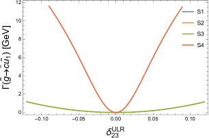
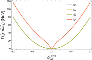
Figure 1: Partial decay width of $\tilde{g}\rightarrow\bar{c}\tilde{u}_{1}$ mode as a function of $\delta_{23}^{ULR}$ (left) and $\delta_{23}^{URR}$ (right).

In Fig. 2 we show the partial decay width of $\tilde{g}\rightarrow\bar{t}\tilde{u}_{1}$ as a function of QFV parameters $\delta^{ULR}_{23}$ (left) and $\delta^{URR}_{23}$ (right). For the first 3 scenarios, $\delta^{ULR}_{23}$ gives negligible contribution to the partial decay width while for S4, its contribution reaches upto 8 $\,\,\mathrm{GeV}$ for the region $(-0.14:0.14)$ as can be seen in the left plot of Fig. 2. We would like to point however that for the point S4, a small interval (-0.83:-0.76) for $\delta_{23}^{QLL}$ is allowed where the partial decay width can reach upto $\approx 36\,\,\mathrm{GeV}$. On the other hand, the right plot in Fig. 2 represent the contributions resulting from $\delta^{URR}_{23}$. Here again almost entire interval is allowed for $\delta^{URR}_{23}$ and its contribution to the partial decay width $\Gamma(\tilde{g}\rightarrow\bar{t}\tilde{u}_{1})$ amounts to $84\,\,\mathrm{GeV}$ for first 2 scenarios and for S3, S4 decay width is $82\,\,\mathrm{GeV}$, $118.9\,\,\mathrm{GeV}$, respectively.

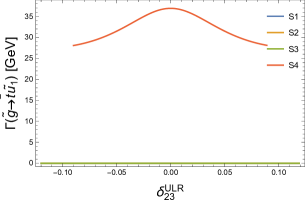
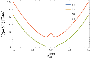
Figure 2: Partial decay width of $\tilde{g}\rightarrow\bar{t}\tilde{u}_{1}$ mode as a function of $\delta_{23}^{ULR}$ (left) and $\delta_{23}^{URR}$ (right).

In Figs. 3 and 4, we show the decay width $\Gamma(\tilde{g}\rightarrow\bar{s}\tilde{d}_{1})$ and $\Gamma(\tilde{g}\rightarrow\bar{b}\tilde{d}_{1})$ respectively, as a function of QFV parameters. The effect of $\delta^{QLL}_{23}$ on $\Gamma(\tilde{g}\rightarrow\bar{s}\tilde{d}_{1})$ is significant and is shown in the upper left plot of Fig. 3 where it can reach upto $6\,\,\mathrm{GeV}$, $4\,\,\mathrm{GeV}$ and $1\,\,\mathrm{GeV}$ for the S1, S2 and S3, respectively. While it can reach upto $19\,\,\mathrm{GeV}$ in S4 for the interval (-0.14:0.14) and upto $92\,\,\mathrm{GeV}$ for the interval (-0.83:-0.76). In the upper right plot of Fig. 3, we show the dependence of $\Gamma(\tilde{g}\rightarrow\bar{s}\tilde{d}_{1})$ on $\delta^{DLR}_{23}$. Here the UFB/CCB constraints on $\delta_{23}^{DLR}$ are very stringent and only a small interval (-0.002,0.002) is allowed for the point S4. In this small interval, the $\Gamma(\tilde{g}\rightarrow\bar{s}\tilde{d}_{1})$ is $2\,\,\mathrm{GeV}$. However for other scenarios, the effect of $\delta^{DLR}_{23}$ on the $\Gamma(\tilde{g}\rightarrow\bar{s}\tilde{d}_{1})$ remains negligible. The effects of $\delta_{23}^{DRR}$ are shown in Fig. 3 (lower center plot). Its contribution in S1, S2, S3 can amount to $75.6\,\,\mathrm{GeV}$ while for the point S4, the partial decay width reaches upto $114\,\,\mathrm{GeV}$.

In the upper left plot of Fig. 4, we have analyzed the $\Gamma(\tilde{g}\rightarrow\bar{b}\tilde{d}_{1})$ as a function of $\delta_{23}^{QLL}$. In the first scenario, the contribution of $\delta^{QLL}_{23}$ can result in the increase of $\Gamma(\tilde{g}\rightarrow\bar{b}\tilde{d}_{1})$ upto $6\,\,\mathrm{GeV}$ under the allowed interval. For S2 and S3 the contribution is $4\,\,\mathrm{GeV}$ and $1\,\,\mathrm{GeV}$, respectively. For the point S4, $\delta^{QLL}_{23}$ gives negative contribution to the $\Gamma(\tilde{g}\rightarrow\bar{b}\tilde{d}_{1})$ in the interval (-0.01,0.01). However for $\delta^{QLL}_{23}>0.01$, the $\Gamma(\tilde{g}\rightarrow\bar{b}\tilde{d}_{1})$ gets positive contributions. The overall effect can reach upto 10 $\,\,\mathrm{GeV}$ depending upon the value of $\delta^{QLL}_{23}$. However, for the interval (-0.83:-0.76), the $\delta^{QLL}_{23}$ gives $\Gamma(\tilde{g}\rightarrow\bar{b}\tilde{d}_{1})=92\,\,\mathrm{GeV}$. In Fig. 4 (upper left plot), we can see the $\Gamma(\tilde{g}\rightarrow\bar{b}\tilde{d}_{1})$ as a function $\delta^{DLR}_{23}$. Due to the stringent constraints on this parameter, its contribution is negligible except in the scenario S4 where it can be as high as $20\,\,\mathrm{GeV}$. As a last step, we show $\Gamma(\tilde{g}\rightarrow\bar{b}\tilde{d}_{1})$ as a function of $\delta^{DRR}_{23}$. The contribution goes upto $76\,\,\mathrm{GeV}$ for the first three scenarios and upto $114\,\,\mathrm{GeV}$ for the scenario S4. We summarize our findings in the Tab. 5 where we show the flavor conserving and FV contributions to the partial decay width of different decay modes of gluino.

To summarize, in spite of strong constraint on QFV parameters coming from BPO and vacuum stability condition, QFV gluinos decays do not only get contributions from LL/RR mixing but LR/RL mixings can also make colossal contributions to the partial decay width. These contributions may have important influence on the experimental searches for gluinos at LHC and future colliders.

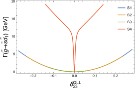
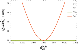
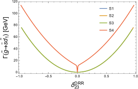
Figure 3: Partial decay width of $\tilde{g}\rightarrow\bar{s}\tilde{d}_{1}$ mode as a function of $\delta_{23}^{QLL}$ (upper left), $\delta_{23}^{DLR}$ (upper right) and $\delta_{23}^{DRR}$ (lower plot).

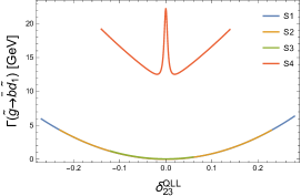
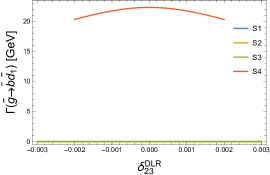
Figure 4: Partial decay width of $\tilde{g}\rightarrow\bar{b}\tilde{d}_{1}$ mode as a function of $\delta_{23}^{QLL}$ (upper left), $\delta_{23}^{DLR}$ (upper right) and $\delta_{23}^{DRR}$ (lower plot).

$\tilde{g}\rightarrow\bar{s}\tilde{d}_{1}$
Point	No FV	$\delta_{23}^{QLL}$	$\delta_{23}^{DLR}$	$\delta_{23}^{DRR}$
$S1$	$0$	$6.39$	$0.61\times 10^{-3}$	$75.6$
$S2$	$0$	$4.3$	$0.61\times 10^{-3}$	$75.6$
$S3$	$0$	$1.16$	$0.61\times 10^{-3}$	$75.6$
$S4$	$0$	$19.18$	$2.06$	$113.6$
$\tilde{g}\rightarrow\bar{b}\tilde{d}_{1}$
Point	No FV	$\delta_{23}^{QLL}$	$\delta_{23}^{DLR}$	$\delta_{23}^{DRR}$
$S1$	$0$	$6.35$	$0.16\times 10^{-2}$	$75.61$
$S2$	$0$	$4.32$	$0.10\times 10^{-1}$	$75.61$
$S3$	$0$	$1.22$	$0.50\times 10^{-1}$	$75.61$
$S4$	$22.29$	$19.21$	$20.29$	$113.7$
$\tilde{g}\rightarrow\bar{c}\tilde{u}_{1}$
Point	No FV	$\delta_{23}^{QLL}$	$\delta_{23}^{ULR}$	$\delta_{23}^{URR}$
$S1$	0	0	1.117	80.2
$S2$	0	0	1.17	80.2
$S3$	0	0	1.17	78.57
$S4$	0	0	11.6	116.68
$\tilde{g}\rightarrow\bar{t}\tilde{u}_{1}$
Point	No FV	$\delta_{23}^{QLL}$	$\delta_{23}^{ULR}$	$\delta_{23}^{URR}$
$S1$	0	0	0	83.9
$S2$	0	0	0	83.9
$S3$	0	0	0	82.3
$S4$	36.9	0	28.06	119

Table 5: Partial decay width of $\tilde{g}\rightarrow\bar{s}\tilde{d}_{1}$, $\tilde{g}\rightarrow\bar{b}\tilde{d}_{1}$, $\tilde{g}\rightarrow\bar{c}\tilde{u}_{1}$ and $\tilde{g}\rightarrow\bar{t}\tilde{u}_{1}$ with and without flavor violation for the selected parameter points shown in Tab. 1.

5 Conclusions

Supersymmetry (SUSY), in spite of being one of the best candidate beyond the Standard Model (SM), still remains undetected. For SUSY searches at the LHC and future colliders, it is important to study sparticle decays, particularly the decays of the strongly interacting SUSY particles like squarks and gluinos. On the other hand, limits on the sparticle masses are getting higher and higher with each passing day. For example, gluino masses $\leq$ 1900 $\,\,\mathrm{GeV}$ are excluded  [7]. It is therefore, important to study gluino decays with high precison. In this paper we have investigated the effect of squark flavor mixing, parameterized in terms of $\delta_{ij}^{FAB}$ parameters, on the quark flavour violating decays of gluinos into lightest squarks $(\tilde{g}\rightarrow\overline{c}\tilde{u}_{1},$ $\tilde{g}\rightarrow\overline{t}\tilde{u}_{1},$ $\tilde{g}\rightarrow\overline{s}\tilde{d}_{1},$ $\tilde{g}\rightarrow\overline{b}\tilde{d}_{1})$.

We have analyzed the effect of squark mixing in the LL, LR/RL and RR part of the squarks mass matrices on partial decay width of $\tilde{g}\rightarrow q\tilde{q}$. We choose four reference scenarios (with a slight modification in the $M_{A}$), first studied in [22], with the corresponding constraints on the flavor violating (FV) deltas coming from B Physics Observables (BPO). For the said scenerios, we have calculated the constraints on $\delta_{ij}^{FLR,FRL}$, using charge and color breaking minima (CCB) and unbounded from below (UFB) minima. It is thereby observed that the constraints from CCB and UFB are more stringent than the ones obtained via BPO. While it is true that the mixng in the RR part of the squarks mass matrices gives the highest contributions ranging from $75-120\,\,\mathrm{GeV}$, we find however that the mixing in the LL and LR/RL sector can also be important. For instance, for $\delta^{QLL}_{23}$, the $\Gamma(\tilde{g}\rightarrow\overline{s}\tilde{d}_{1})=92\,\,\mathrm{GeV}$ for some parameter points. Similarly $\delta^{ULR}_{23}$ can contribute $\approx 12\,\,\mathrm{GeV}$ to $\Gamma(\tilde{g}\rightarrow\overline{c}\tilde{u}_{1})$ and $\approx 8\,\,\mathrm{GeV}$ to $\Gamma(\tilde{g}\rightarrow\overline{t}\tilde{u}_{1})$. This analysis shows the importance of QFV parameters which could have an important influence on the search for gluinos and the determination of the MSSM parameters at HL-LHC or HE-LHC.

Acknowledgments

We would like to thank Sven Heinemeyer and Mario E. Gomez for their helpful suggestions during the preparation of this manuscript.

References

• [1] Hans Peter Nilles. Supersymmetry, Supergravity and Particle Physics. Phys. Rept., 110:1–162, 1984.
• [2] Howard E. Haber and Gordon L. Kane. The Search for Supersymmetry: Probing Physics Beyond the Standard Model. Phys. Rept., 117:75–263, 1985.
• [3] Riccardo Barbieri. Looking Beyond the Standard Model: The Supersymmetric Option. Riv. Nuovo Cim., 11N4:1–45, 1988.
• [4] S.L. Glashow. Partial Symmetries of Weak Interactions. Nucl. Phys., 22:579–588, 1961.
• [5] Steven Weinberg. A Model of Leptons. Phys. Rev. Lett., 19:1264–1266, 1967.
• [6] Jeffrey Goldstone, Abdus Salam, and Steven Weinberg. Broken Symmetries. Phys. Rev., 127:965–970, 1962.
• [7] Georges Aad et al. Search for new phenomena in final states with large jet multiplicities and missing transverse momentum using $\sqrt{(}s)=13$ TeV proton$-$proton collisions recorded by ATLAS in Run 2 of the LHC. 8 2020.
• [8] M. Arana-Catania, S. Heinemeyer, M.J. Herrero, and S. Penaranda. The Higgs sector of the NMFV MSSM at the ILC. In International Workshop on Future Linear Colliders (LCWS11), pages 336–341, Hamburg, 1 2012. DESY.
• [9] M. Arana-Catania, S. Heinemeyer, and M.J. Herrero. New Constraints on General Slepton Flavor Mixing. Phys. Rev. D, 88(1):015026, 2013.
• [10] M.E. Gómez, T. Hahn, S. Heinemeyer, and M. Rehman. Higgs masses and Electroweak Precision Observables in the Lepton-Flavor-Violating MSSM. Phys. Rev. D, 90(7):074016, 2014.
• [11] M.E. Gomez, S. Heinemeyer, and M. Rehman. Effects of Sfermion Mixing induced by RGE Running in the Minimal Flavor Violating CMSSM. Eur. Phys. J. C, 75(9):434, 2015.
• [12] M.E. Gómez, S. Heinemeyer, and M. Rehman. Quark flavor violating Higgs boson decay h$\to\bar{b}$s+b$\bar{s}$ in the MSSM. Phys. Rev. D, 93(9):095021, 2016.
• [13] W. Beenakker, R. Hopker, and P.M. Zerwas. SUSY QCD decays of squarks and gluinos. Phys. Lett. B, 378:159–166, 1996.
• [14] S.Y. Choi, M. Drees, A. Freitas, and P.M. Zerwas. Testing the Majorana Nature of Gluinos and Neutralinos. Phys. Rev. D, 78:095007, 2008.
• [15] M. Kramer, E. Popenda, M. Spira, and P.M. Zerwas. Gluino Polarization at the LHC. Phys. Rev. D, 80:055002, 2009.
• [16] Tobias Hurth and Werner Porod. Flavour violating squark and gluino decays. JHEP, 08:087, 2009.
• [17] A. Bartl, K. Hidaka, K. Hohenwarter-Sodek, T. Kernreiter, W. Majerotto, and W. Porod. Impact of squark generation mixing on the search for gluinos at LHC. Phys. Lett. B, 679:260–266, 2009.
• [18] A. Bartl, H. Eberl, E. Ginina, B. Herrmann, K. Hidaka, W. Majerotto, and W. Porod. Flavour violating gluino three-body decays at LHC. Phys. Rev. D, 84:115026, 2011.
• [19] S. Heinemeyer and C. Schappacher. Gluino Decays in the Complex MSSM: A Full One-Loop Analysis. Eur. Phys. J. C, 72:1905, 2012.
• [20] Helmut Eberl, Elena Ginina, and Keisho Hidaka. Two-body decays of gluino at full one-loop level in the quark-flavour violating MSSM. Eur. Phys. J. C, 77(3):189, 2017.
• [21] J.A. Casas and S. Dimopoulos. Stability bounds on flavor violating trilinear soft terms in the MSSM. Phys. Lett. B, 387:107–112, 1996.
• [22] M. Arana-Catania, S. Heinemeyer, and M.J. Herrero. Updated Constraints on General Squark Flavor Mixing. Phys. Rev. D, 90(7):075003, 2014.
• [23] Thomas Hahn. Generating Feynman diagrams and amplitudes with FeynArts 3. Comput. Phys. Commun., 140:418–431, 2001.
• [24] T. Hahn and M. Perez-Victoria. Automatized one loop calculations in four-dimensions and D-dimensions. Comput. Phys. Commun., 118:153–165, 1999.
• [25] M. Tanabashi et al. Review of Particle Physics. Phys. Rev. D, 98(3):030001, 2018.