Impact of non-tidal station loading in LLR

Abstract

Lunar Laser Ranging (LLR) measures the distance between observatories on Earth and retro-reflectors on Moon since 1970. In this paper, we study the effect of non-tidal station loading (NTSL) in the analysis of LLR data. We add the non-tidal loading effect provided by three data centres: the German Research Centre for Geosciences (GFZ), the International Mass Loading Service (IMLS) and EOST loading service of University of Strasbourg in France, as observation level corrections of the LLR observatories in our analysis. This effect causes deformations of the Earth surface up to the centimetre level. Its addition in the Institute of Geodesy (IfE) LLR model, it leads to a change in the uncertainties (3-$\sigma$ values) of the station coordinates resulting in up to a 0.60% improvement, an improvement in the post-fit LLR residuals of up to 9%, and a decrease in the power of the annual signal in the LLR post-fit residuals of up to 57%.

Keywords— lunar laser ranging; non-tidal loading; station displacements

1 Introduction

Lunar laser ranging (LLR) is the measurement of round trip travel times of short laser pulses between observatories on the Earth and retro-reflectors on the Moon. There are five retro-reflectors on the Moon, and measurements have primarily been carried out from six observatories on Earth, details of which are given in Table 1. For each returning laser pulse, the round-trip travel time (Earth-Moon-Earth) is observed. As the amount of signal loss of the laser pulse is enormous, it is necessary to collect measurements for 1 to 15 minutes. Of these, a statistically secured mean value is computed, a so called normal point (NP). Details of the LLR measurement process can be found, for example, in Murphy, (2013) and Müller et al., (2019). The NP is treated as the actual observable of LLR. The recent NP are provided by the CDDIS and be downloaded from the website. The LLR data is available from 1969, and at present, the Institute of Geodesy (IfE) LLR dataset contains 26839 NPs, and spans from 1970 - 2019.

Table 1: Details of LLR observatories and their observations used within IfE normal point (NP) file.

Name	Abbreviation	NPs	Timespan
Observatoire de la Côte d’Azur, Grasse, France	OCA	16298	1984 - 2005, 2009 - 2019
Matera Laser Ranging Observatory, Matera, Italy	MLRO	240	2003 - 2004, 2010 - 2019
Wettzell Laser Ranging System, Wettzell, Germany	WLRS	48	1994, 1996, 2018 - 2019
Apache Point Observatory Lunar Laser-ranging Operation, in New Mexico, USA	APOLLO	2585	2006 - 2016
Lunar Laser Ranging Experiment Observatory, Hawaii, USA	LURE	755	1984 - 1990
McDonald Laser Ranging Station, Texas, USA	McDonald	3070	1970 - 1985
	MLRS1	710	1983 - 1988
	MLRS2	3133	1988 - 2013

As LLR has the longest observation time series of all space geodetic techniques (Müller et al., , 2019), it allows the determination of a variety of parameters of the Earth–Moon dynamics, for example, the mass of the Earth–Moon system, the lunar orbit and libration parameters (Williams et al., , 2013; Pavlov et al., , 2016); and it leads to improvements in the solar system ephemerides (Folkner et al., , 2014), terrestrial and celestial reference frames and coordinates of observatories and reflectors (Müller et al., , 2009; Hofmann et al., , 2018), selenophysics (Murphy, , 2013; Hofmann, , 2017; Viswanathan et al., , 2019), and gravitational physics, i.e. tests of Einstein’s relativity theory, for example, strong equivalence principle, metric or preferred-frame effects, variation of the gravitational constant (Williams et al., , 2006; Müller et al., , 2012; Hofmann and Müller, , 2018; Zhang et al., , 2020). LLR can also be used to provide tests of Earth orientation parameters (Biskupek, , 2015; Hofmann et al., , 2018).

The Earth’s crust is continuously deforming, due to which the positions of the observatories on Earth change over time. Various geophysical process contribute to the deformation of the crust, which can be estimated by different models. The 2010 conventions of the International Earth Rotation and Reference Systems Service (IERS) (Petit and Luzum, , 2010) provide details of the models recommended to be used for instantaneous calculation of deformations of reference points on the crust.

The deformations of the crust due to redistribution of masses in atmospheric, ocean, and land water mass has both tidal and non-tidal loading (NTL) components. The IERS 2010 conventions do not recommend the addition of NTL deformations in the calculation of the displacement of a reference points. The IERS, however, established the Global Geophysical Fluids Center (GGFC) in 1998, which has different bureaus responsible for research and data provision related to the redistribution of masses in atmosphere, oceans, and hydrological (land water) systems. These bureaus, amongst other products, provide time series of NTLs over different time spans, based on calculations using numerical weather models and Green’s functions (Farrell, , 1972; Dill and Dobslaw, , 2013; Petrov, , 2015), which can be added as observation level corrections in the calculation of the instantaneous position of a reference site.

NTL plays a special role in optical observation techniques (satellite laser ranging (SLR) and LLR) as their observations can only be performed during clear sky conditions, creating a difference in their results in comparison with microwave observation techniques (such as Very Long Baseline Interferometry (VLBI) and Global Navigation Satellite Systems (GNSS)) (Otsubo et al., , 2004; Sośnica et al., , 2013; Bury et al., , 2019). This weather-dependent-effect on the results is called the Blue-Sky effect. The accuracy of the loading effect due to NTL, as pointed out by Glomsda et al., (2020), has improved over the past years due to the improved accuracy of the numerical weather models used for its calculation (Jungclaus et al., , 2013; Gelaro et al., , 2017; Hersbach et al., , 2018; Dill and Dobslaw, , 2013), and therefore addition of NTL can be beneficial in geodetic analyses.

The effect of NTL has already been studied in VLBI ((Schuh et al., , 2004; Glomsda et al., , 2020), and others), GNSS ((Boy and Lyard, , 2008; Dach et al., , 2010; van Dam et al., , 2012; Nordman et al., , 2015; Mémin et al., , 2020), and others), and SLR ((Sośnica et al., , 2013; Bury et al., , 2019), and others). Their results have mentioned that addition of displacements due to NTL leads to an improvement, most significantly in reduction of seasonal signals.

In this paper, Section 2 describes the NTL and its components and compares the data from different data centres for all loading components. Section 3 contains the results of implementing all loadings of NTL from different data centres in LLR analysis. Section 4 gives the conclusions and addresses further aspects in this context.

2 Non-tidal loading datasets

As mentioned in section 1, the redistribution of masses in atmosphere, ocean, and land water causes displacements which have NTL components. These displacements for any particular point $X$ are calculated based on Farrell, (1972), which converts pressure differences from a mean pressure value to horizontal and vertical displacement components. The calculation involves integration over an area $A$ around the point $X$, weighting the pressure at other points $X^{\prime}$ within the area using a Green’s function. The Green’s function is dependent on the angular distance between the point $X$ and $X^{\prime}$, given as:

$$Gr(\cos{\beta})=\frac{GR}{g}\sum_{n=1}^{\infty}h_{n}^{\prime}P(\cos{\beta}),$$ (1)

where $\beta$ is the angular distance between point $X$ and $X^{\prime}$, $h_{n}^{\prime}$ is the load Love number, $P(\cos{\beta})$ the Legendre polynomial, $G$ the gravitational constant, $g$ the mean surface gravity, and $R$ the mean radius of the Earth.

The deformation (here, up component) at point $X$ is then calculated as:

$$\zeta_{up}(X,t)=\int_{A}\frac{\Delta p}{g}Gr(\cos{\beta})dA,$$ (2)

where $\Delta p$ is the pressure difference at the point of integration, $dA$ is surface element defined by $X$ and $X^{\prime}$. The procedure for displacement calculation due to NTL is described in detail by Petrov and Boy, (2004); Dill and Dobslaw, (2013); Petrov, (2015) and others.

The pressure values are obtained from various different numerical weather models (NWMs), which consider different effects for their own calculation.

According to the GGFC website, the NTL data is provided by the following official centres:

1. EOST loading service, Univerity of Strasbourg, France,

2. GGOS Atmosphere at Vienna (VMF), Technical University Vienna, Austria,

3. German Research Centre for Geosciences (GFZ), Potsdam, Germany, and

4. University of Luxembourg (ULux), Luxembourg.

Additionally, NTL data can also be obtained from the International Mass Loading Service (IMLS). Not all data centres provide all three non-tidal loadings (atmosphere: NTAL, ocean: NTOL, and hydrological: HYDL), and some of the data centres provide loadings calculated from more than one NWM. In Table 2, we give a list of the loadings and their corresponding NWMs considered in this study.

Table 2: Details of the loading components and their corresponding numerical weather models (NWM) of different data centres.

Dataset	Timespan	Loading Component	NWM	Temporal Resolution
GFZ	1976 - present	Atmospheric	ECMWF	3h or 24h
		Oceanic	MPIOM	3h or 24h
		Hydrological	LSDM	24h
		Sea level	LSDM + ECMWF	24h
IMLS	1980 - present	Atmospheric	MERRA2	6h
		Oceanic	MPIOM	3h
		Hydrological	MERRA2	3h
EOST	1980 - present	Atmospheric	MERRA2	1h
		Oceanic1	ECCO2	24h
		Hydrological	MERRA2	1h
VMF	1994 - present	Atmospheric	ECWMF	6h
ULux	1980 - 2015	Atmospheric	NCEP	6h

• starting 1992
  

• ECMWF: European Centre for Medium-Range Weather Forecasts
  

• MPIOM: Max-Planck-Institute Global Ocean/Sea-Ice Model
  

• LSDM: Land Surface Discharge Model
  

• MERRA2: Modern-Era Retrospective analysis for Research and Applications, Version 2
  

• NCEP: National Center for Environmental Protection (USA)
  

• ECCO2: Estimating the Circulation and Climate of the Ocean, version 2
  

For IMLS and EOST dataset, in addition to the the loadings from the NWMs mentioned in Table 2, other options are also available. However, the other NWMs have limitations, such as a shorter time span, discontinued NWM, et cetera, and therefore were not used for this study.

As it can be seen from Table 2, the datasets from different centres have some differences in the temporal resolution and the models used for their computation. Slight differences in the displacements could also occur due to the procedure used to compute the integral to get them. All datasets use Green’s functions to compute the NTL displacements, however, the GFZ and IMLS mention two special approaches to solve the convolution integrals (like Eq 2). The GFZ uses a patched version to be able to reduce the computation time to obtain the displacements (Dill and Dobslaw, , 2013). It applies a high spatial resolution for nearby pressure fields and a lower spatial resolution for those far away, which are combined used fast interpolation techniques. The IMLS uses a spherical harmonic transformation approach to solve the integral. The algorithm for this transformation is described in (Petrov, , 2015).

2.1 Non-tidal atmospheric loading

The effect of NTAL has been extensively studied within different space geodetic techniques, such as van Dam et al., (1994); Tregoning and Watson, (2009, 2011); Sośnica et al., (2013); König et al., (2018); Bury et al., (2019) and others. The atmospheric pressure loading (APL) over the Earth has a tidal and non-tidal component. Both components of APL are modelled separately, and can cause up to cm level deformations of the Earth surface (Petrov and Boy, , 2004).

The application of NTAL commonly assumes the response of ocean to the atmospheric loading to be that of an inverted barometer (IB), i.e. an increase in atmospheric pressure at any point of the ocean is directly compensated by an equivalent decrease in sea level at this point Petrov and Boy, (2004); Glomsda et al., (2020). This also leads to a decrease in ocean bottom pressure of equal size. Height variations of the ocean for periods longer than 5–20 days are successfully represented by this model, however, for shorter periods this model does not capture the height variations correctly (Wunsch and Stammer, , 1997). According to Van Dam and Wahr, (1987), points on Earth within a few hundred kilometres of the coast are affected by the choice of the oceanic response (IB or non-inverted barometer (NIB)) to APL, showing a higher value of deformation for NIB than the deformation at the same point calculated by an IB model. Inland observation points are not significantly affected by the choice of the ocean response model.

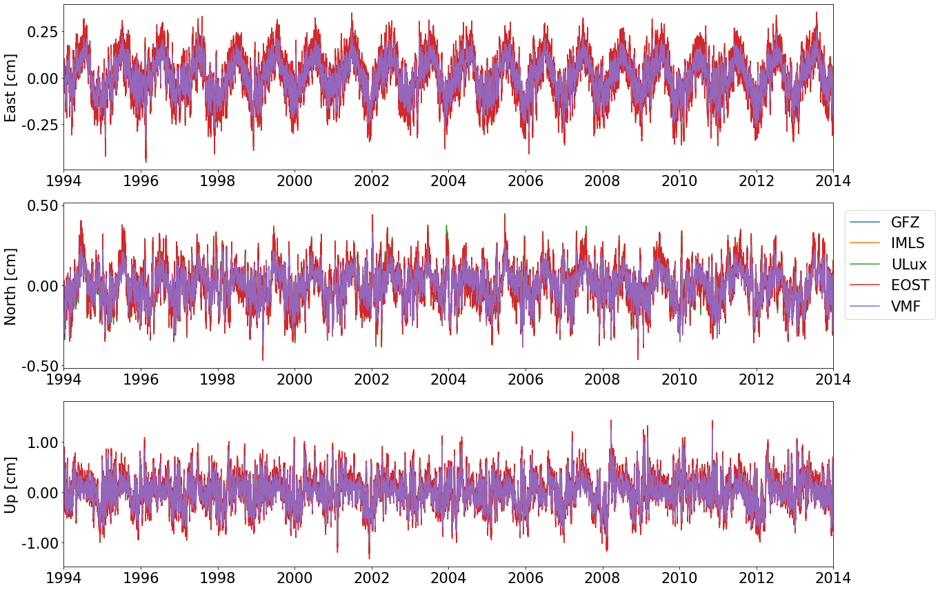
Figure 1: Effect of NTAL at the OCA station from 1994 to 2014 for GFZ, IMLS, ULux, EOST, and VMF datasets.

From the Figure 1, it can be seen that the NTAL has the highest effect in the up component of the displacement, ranging between $\pm$1 cm. The horizontal displacement due to NTAL lies between $\pm$0.45 cm (North) and between $\pm$0.3 cm (East). The effect of NTAL has the highest contribution of all NTL effects for inland observatories. For NTAL, all input time series almost completely overlap each other for all (Up, North, East) components, with the exception of VMF, which shows differences in the horizontal components of loading for some stations compared to other datasets. The maximum of these differences, for LLR observatories, are observed for the APOLLO and McDonald stations (not shown), where the differences in the range of the horizontal components of VMF compared to the GFZ dataset are up to 45% for both stations. These differences could be due to different land-sea masks, resolution, weather models, computation method, et cetera. However, as the horizontal components of NTAL are less significant than the vertical components, and as the effect of horizontal components of NTAL is only up to a few millimetres, it is not expected to produce significant differences in the time series of geodetic observations between results obtained from VMF and other NTAL datasets.

2.2 Non-tidal oceanic loading

The ocean water redistribution by atmospheric circulation, inflow and outflow of ocean water, and changes in the total atmospheric mass over the oceans primarily cause NTOL deformations (Glomsda et al., , 2020). It plays an important role in different space geodetic techniques, and its effect has been studied, for example, by Williams and Penna, (2011); van Dam et al., (2012); Mémin et al., (2014); Oreiro et al., (2018); Mémin et al., (2020), and others.

Figures 2 shows the NTOL at the OCA station. All LLR stations show a similar trend for NTOL, i.e. GFZ and IMLS NTOL time series are similar, and the EOST time series differs, but stays within the same range as GFZ and IMLS, $\pm$0.65 cm for Up component, $\pm$0.50 cm for North component, and -0.50 cm to 0.40 cm for East. These differences between datasets can be attributed to the differences in the underlying NWMs used for NTOL calculation. NTOL is most dominant for coastal points. For LLR stations, this effect is observed for LURE station (not shown).

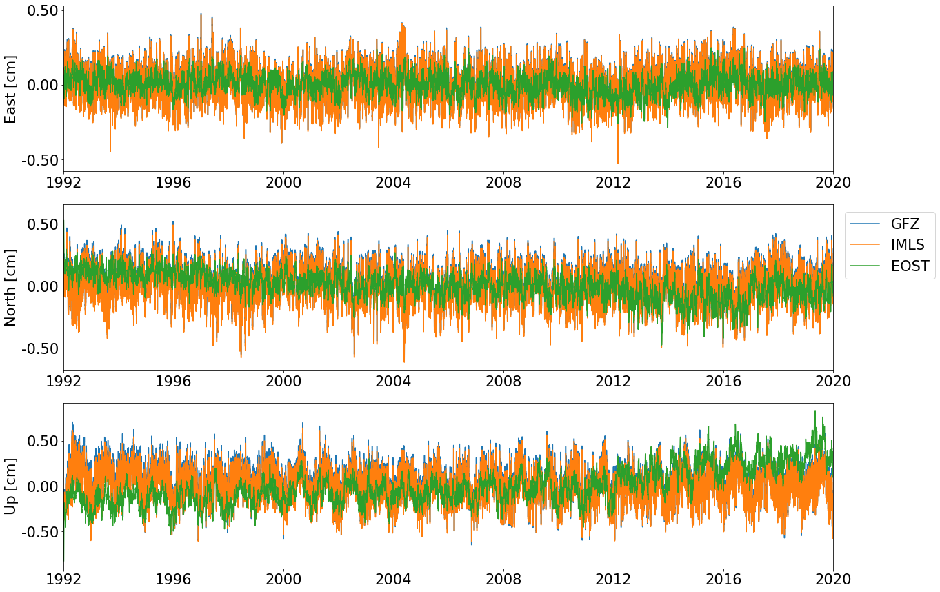
Figure 2: Effect of NTOL at the OCA station from 1992 to 2020 for GFZ, IMLS, and EOST datasets.

2.3 Hydrological loading

HYDL’s effect in space geodetic techniques has been studied by Van Dam et al., (2007); Tregoning et al., (2009); Dill and Dobslaw, (2013); Dill et al., (2018) and others. HYDL is caused by redistribution of continental water mass, such as snow, ground water, et cetera. According to Dill and Dobslaw, (2013), it is most dominating along lakes and river sides, and along the Rocky Mountains (North America).

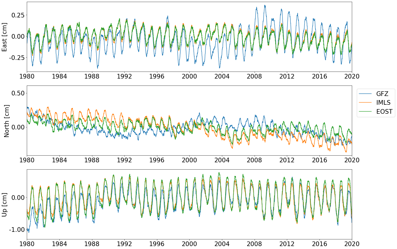
Figure 3: Effect of HYDL at the OCA station from 1980 to 2020 for GFZ, IMLS, and EOST datasets.

Figure 3 show the HYDL loading at the OCA station. All LLR stations show a similar trend for HYDL loading, i.e. EOST and IMLS HYDL time series are similar (ranging between -0.90 cm and 0.75 cm for Up component, -0.35 cm and 0.30 cm for North component, and -0.20 cm and 0.20 cm for East component), however the time series from the GFZ dataset (ranging between -1.20 cm and 0.60 cm for Up component, -0.25 cm and 0.55 cm for North component, and -0.40 cm and 0.35 cm for East component) differs significantly. The differences between the datasets are assumed to be a resultant of differences between their underlying NWMs and the kinds of water mass redistribution considered therein. As pointed out by Glomsda et al., (2020), LSDM continental water storage (GFZ) considers soil moisture, snow accumulation, seasonal runoff from glaciers, and water flow in river channels given as daily states on a 0.5 degree regular global grid (Dill and Dobslaw, , 2013). MERRA2 (IMLS and EOST), on the other hand, includes snow coverage, soil moisture, stream-flow, and observation-based precipitation, given on on 0.625 degree x 0.5 degree grid (Gelaro et al., , 2017).

2.4 Sea level loading

In addition to NTAL, NTOL, and HYDL, the GFZ additionally provides another component of NTL, Sea level loading (SLEL), to be considered. Each single loading model conserves its own total mass, but as the GFZ dataset uses different models for NTAL and HYDL, the global mass is not conserved as the mass exchange between the atmosphere and land is not considered (Thomas et al., , 2020). Therefore, the sea-level varies. Including this change helps obtain a global mass conservation. The SLEL use continental mass from the global hydrological model LSDM, and the atmospheric mass from the model ECMWF. For any point on Earth, the total NTL for GFZ dataset will be the sum of all four loadings. In this study, we consider SLEL as a part of the total NTL at any station for the GFZ dataset, however we do not discuss individual results due to SLEL.

2.5 Degree 1 deformation

Due to the difference in the centre of mass of the Earth to the solid Earth’s centre of mass, the loading deformation can be defined in a centre of figure (CF) frame (realised from the positions of geodetic stations on the solid Earth) or centre of mass (CM) frame (centre of orbiting satellites). This is defined by the choice of degree-one load Love numbers, which enter the Green’s function summation (Petrov and Boy, , 2004; Dill and Dobslaw, , 2013; Petrov, , 2015). For further details on the differences between CM and CF, we refer the reader to (Sun, , 2017). The loading obtained from the summation is then defined in the reference frame chosen for the load Love numbers. In our LLR analysis, the a-priori station positions are aligned to CM frame and therefore the loadings from all datasets used within this study were chosen in the CM frame.

3 Impact of NTL on LUNAR

IfE’s standard lunar laser ranging analysis software, LUNAR (see, for details (Müller et al., , 2014) and latest version (Hofmann and Müller, , 2018)), did not include any non-tidal loading effects so far. Within LUNAR, an adjustment is performed following the Gauss-Markov model, using over 250 parameters, such as the dynamical parameters for the Moon, LLR station and reflector coordinates, et cetera. The post-fit residuals are then obtained after the adjustment. In current version of LUNAR, the a-priori station coordinates are taken from ITRF2014 (Altamimi et al., , 2016), with the exception of coordinates for the APOLLO station which were personally communicated to us by Prof. Thomas Murphy; and the a-priori reflector coordinates are taken from (Williams, , 2008) and (Murphy et al., , 2010). Table 3 shows a list of models used within LUNAR, which are all based on the IERS 2010 conventions (Petit and Luzum, , 2010).

Table 3: List of models used to compute the standard solution.

Effect	Model
Tidal atmospheric delay	Ray and Ponte (2003)
Tidal ocean loading	FES 2004
Solid Earth tides	IERS 2010
Deformation due to polar motion	IERS 2010 mean pole model
Ocean pole tides	Desai (2002)
Tropospheric delay	Mendes and Pavlis (2004)

In this study, the effect of NTLs, described in section 2, was added to LUNAR to analyse the effect on various results. A degree 10 Lagrange interpolation was performed on the time series of all individual loadings in all datasets. The NTL effects were added as corrections to the station coordinates at observation level. To compare if the NTL contribution leads to an improvement or a deterioration, the reference results, hereon be referred to as ‘standard’ solution, are compared to the results obtained upon addition of NTL in LUNAR.

The timespan in which the NTL are available, as mentioned in Table 2, are different for the datasets and loadings. For sake of comparison between the results obtained from all datasets, the results shown in this paper are for the case when loadings are added only in the timespan 1980 to present, and loadings with shorter timespans (i.e. NTOL from EOST, NTAL from VMF and ULux) are not added.

In the results, “NTSL” refers to the solution with all loadings of any dataset applied together in the analysis, i.e. a combination of NTAL, NTOL, HYDL, and SLEL for GFZ; a combination of NTAL, NTOL, and HYDL for IMLS; and a combination of NTAL and NTOL for EOST.

3.1 One way weighted root mean square of the residuals

To ascertain if the added effect of NTL in LLR analysis proves to be useful or not, we calculated the change in the one way annually averaged weighted root mean square of the post-fit LLR residuals obtained from LUNAR, henceforth referred to as WRMS.

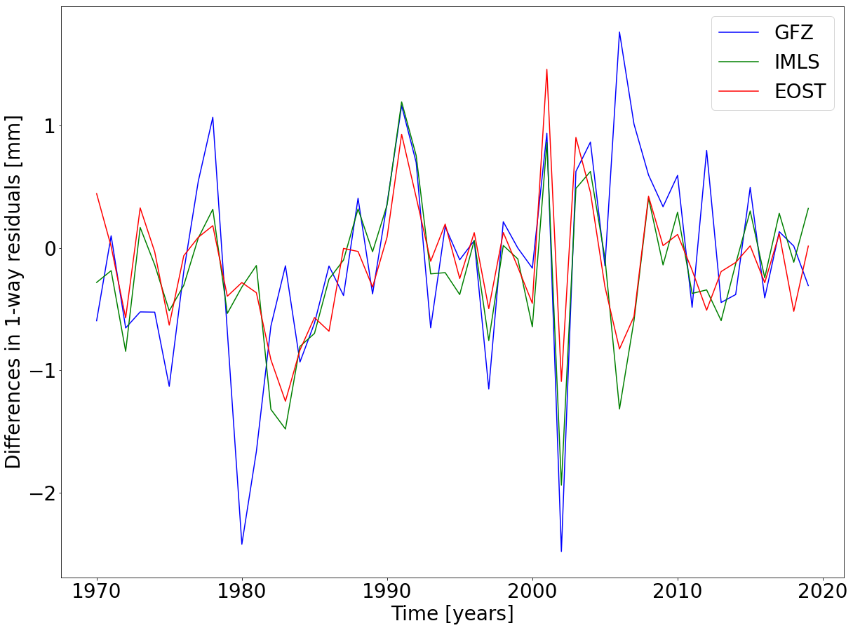
Figure 4: WRMS for GFZ and IMLS NTSL subtracted from standard solution, for all LLR stations.

Figure 4 shows the magnitude of differences (standard solution minus NTL solutions) obtained in the WRMS (negative values mean lower residuals, and therefore better), showing the effect impacting up to a few millimetres. Figure 5 to 8 show the percentage change in WRMS obtained from LUNAR when adding NTL for all LLR stations (positive change means improvement, i.e. lower value of WRMS).

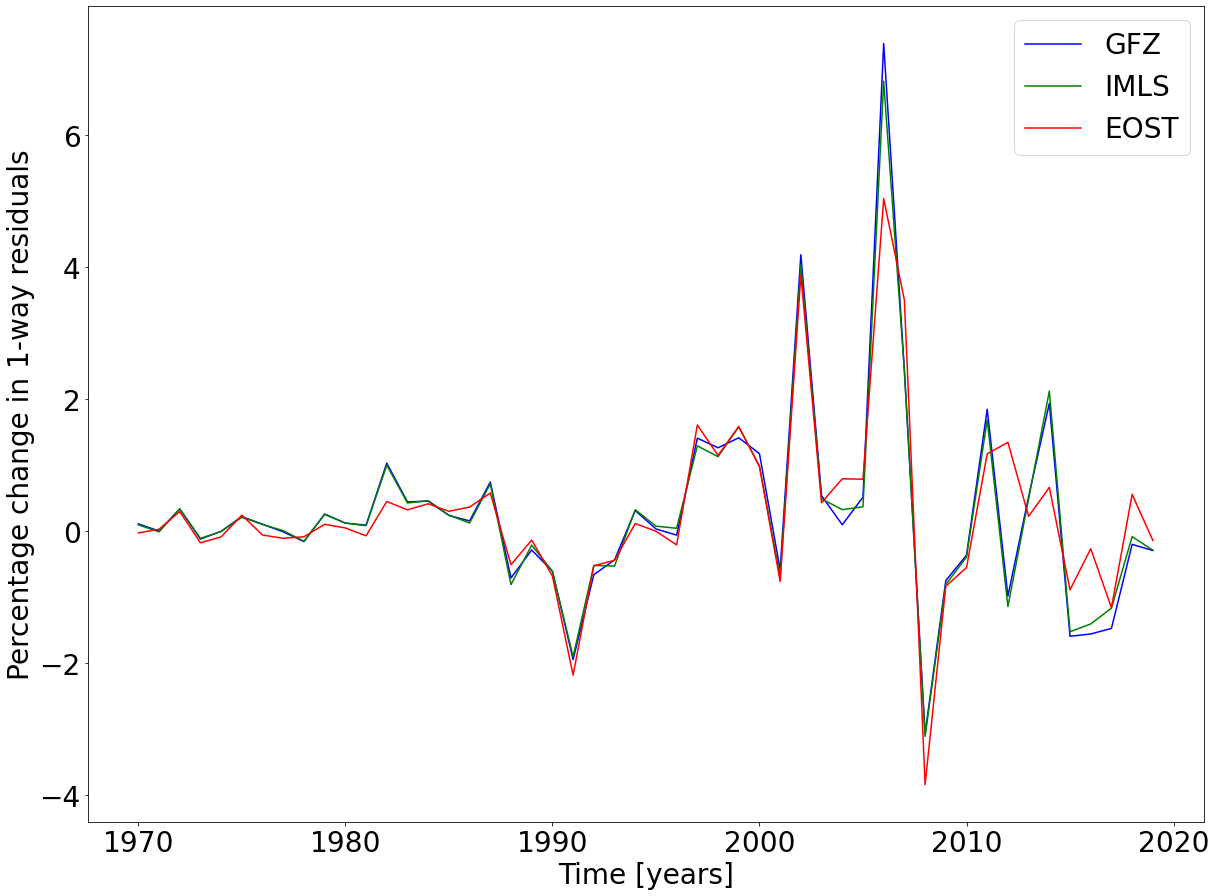
Figure 5: Percentage change in WRMS for the GFZ, IMLS, and EOST NTAL solutions compared to the standard solution for all LLR stations.

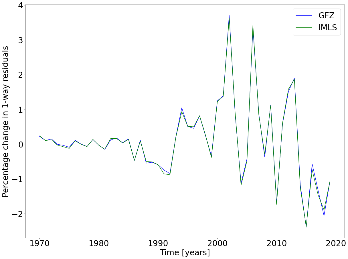
Figure 6: Percentage change in WRMS for the GFZ and IMLS NTOL solutions compared to the standard solution for all LLR stations.

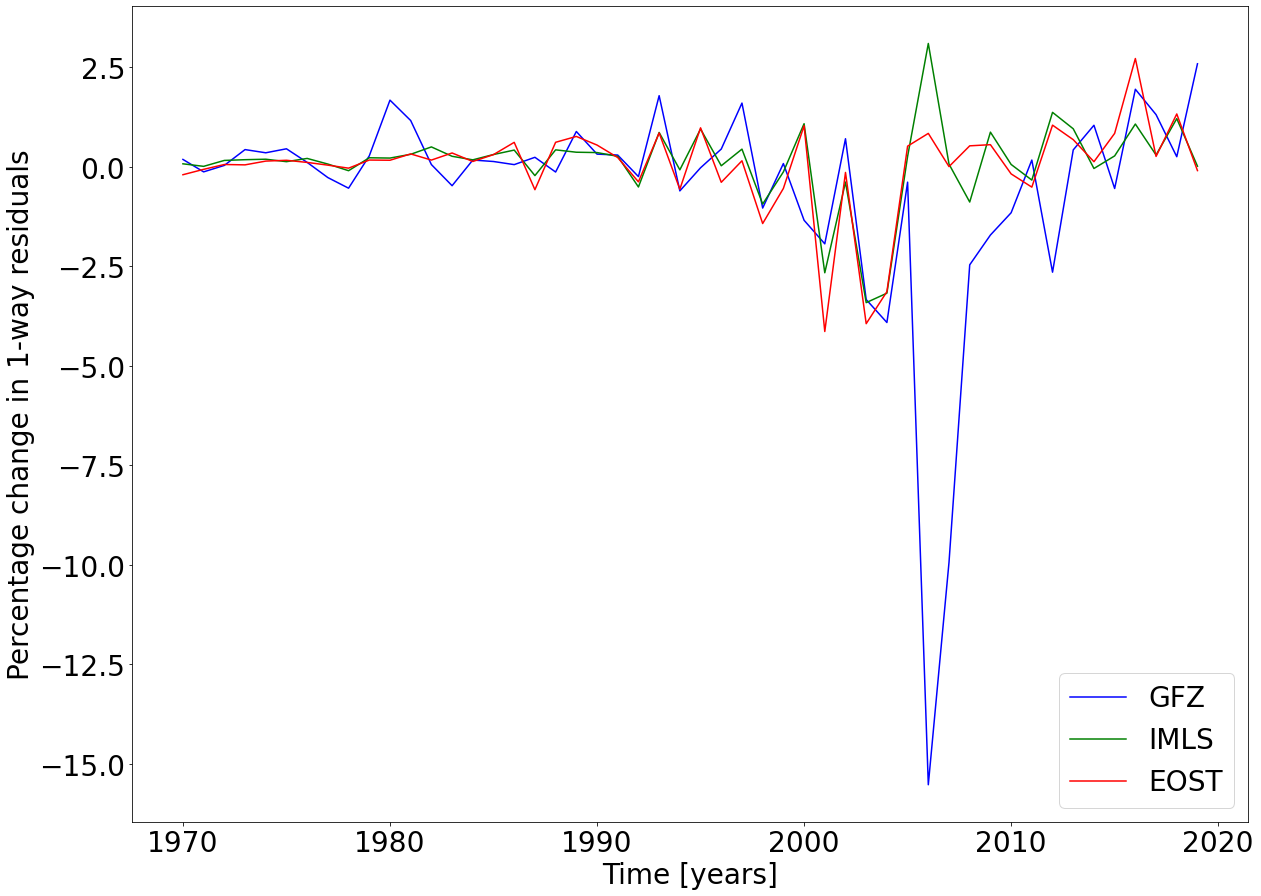
Figure 7: Percentage change in WRMS for the GFZ, IMLS, and EOST HYDL solutions compared to the standard solution for all LLR stations.

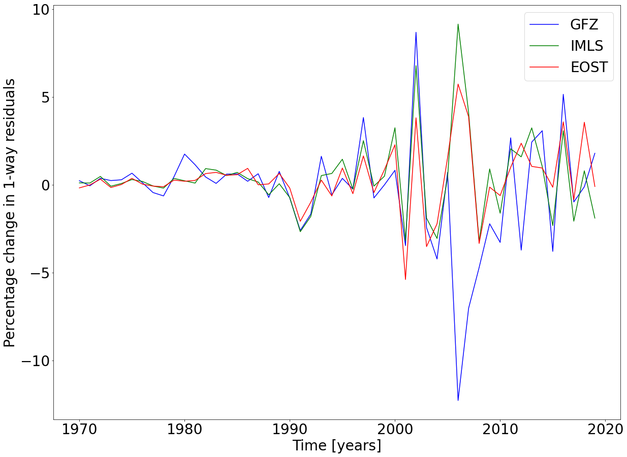
Figure 8: Percentage change in WRMS for the GFZ, IMLS, and EOST NTSL solutions compared to the standard solution for all LLR stations.

From Figure 5, it can be seen that the effect of NTAL’s addition in LUNAR has similar effects on the post-fit residuals for loadings from all three data centres; the results obtained from IMLS and GFZ datasets almost overlap each other, and EOST is in close agreement. The percentage change due to NTAL from EOST lies between 4% deterioration and 5% improvement, and due to NTAL from GFZ and IMLS lies between 3% deterioration and 7.5% improvement. A mean value of percentage change per year over all 50 years of data shows an improvement of approximately 0.27% for all datasets in NTAL. For NTOL (see Figure 6), the percentage change over the years from IMLS and GFZ datasets overlap each other, ranging between 2.5% deterioration and 3.7% improvement, producing an overall improvement in the mean value of percentage change over 50 years of 0.09%. The percentage change due to HYDL is different for all datasets, lying between 15.5% deterioration and 2.6% improvement for GFZ, between 3.5% deterioration and 3% improvement for IMLS, and between 4% deterioration and 3% improvement for EOST. Overall in the LLR timespan, GFZ shows a deterioration of 0.58%; however, the HYDL datasets from IMLS and EOST show an improvement in the mean change over the years of 0.10% and 0.02%, respectively (see Figure 8). This difference in the results between the HYDL datasets is expected due to the different input time series, as shown by Figure 3.

When combining all loadings from each dataset (see Figure 8), the range of change differs for each data set. For GFZ the change ranges between 12% deterioration and 9% improvement, for IMLS between 3% deterioration and 9% improvement, and for EOST between 5% deterioration and 6% improvement. The mean value of percentage change over all years is 0.43% for EOST (improvement), 0.35% for IMLS (improvement), and -0.34% for GFZ (deterioration). Figure 5 to 8 show a higher value of percentages in the last thirty years because of better laser systems which help obtain a lower value of the LLR residuals in the recent years.

Table 4: Mean values of WRMS for the standard solution (Std), and for the solutions with GFZ, IMLS, and EOST datasets for all LLR stations and loadings.

Observatory	Dataset	GFZ	IMLS	EOST	Observatory	Dataset	GFZ	IMLS	EOST
		[mm]	[mm]	[mm]			[mm]	[mm]	[mm]
APOLLO	Std	15.02	15.02	15.02	LURE	Std	64.79	64.79	64.79
	NTAL	14.91	14.92	14.91		NTAL	64.67	64.72	64.41
	NTOL	14.95	14.95	-		NTOL	65.11	65.10	-
	HYDL	15.50	14.95	14.97		HYDL	64.57	64.72	64.54
	NTSL	15.42	14.77	14.84		NTSL	64.47	64.68	64.22
McDonald	Std	167.77	167.77	167.77	OCA	Std	38.81	38.81	38.81
	NTAL	167.41	167.42	167.57		NTAL	38.78	38.80	38.76
	NTOL	167.63	167.64	-		NTOL	38.79	38.79	-
	HYDL	167.47	167.49	167.64		HYDL	38.69	38.71	38.69
	NTSL	167.20	167.27	167.45		NTSL	38.60	38.67	38.64
MLRS1	Std	104.98	104.98	104.98	MLRO	Std	31.11	31.11	31.11
	NTAL	104.21	104.25	104.33		NTAL	30.88	30.86	30.82
	NTOL	104.93	104.95	-		NTOL	31.42	31.40	-
	HYDL	104.71	105.01	105.10		HYDL	30.71	30.91	30.79
	NTSL	103.99	104.39	104.46		NTSL	30.58	30.88	30.50
MLRS2	Std	41.26	41.26	41.26	WRLS	Std	44.19	44.19	44.19
	NTAL	41.27	41.26	41.28		NTAL	42.68	42.78	44.16
	NTOL	41.18	41.20	-		NTOL	43.84	43.92	-
	HYDL	41.18	40.87	40.99		HYDL	45.08	45.06	44.11
	NTSL	41.24	40.89	41.02		NTSL	43.15	43.18	44.08

Table 4 shows the mean values of the WRMS obtained for the standard solution, and for solutions with all individual NTL effects, for each station individually. From the table, it can be noticed that HYDL from GFZ shows a deterioration for APOLLO and WLRS stations, but an improvement for the other stations; however, as the magnitude of the deterioration is higher than the magnitude of the improvement, the loading shows an overall deterioration. On the other hand, HYDL from both EOST and IMLS show an improvement in the mean WRMS values of the residuals for all stations except MLRS1 and WLRS. For the the OCA station, which has the highest contribution of NPs (60.73% of NP data), the performance of HYDL is similar solutions from all three datasets. As the APOLLO station station contributes 9.63% of NP data, the deterioration of the WRMS there plays a critical role in LLR analysis. The other loadings from all datasets mostly show an improvement in the mean WRMS values of the residuals.

Figure 8 shows significant deterioration when adding the GFZ HYDL dataset. However, from Table 4, it can be seen that GFZ HYDL improves the mean WRMS for all stations except APOLLO and WLRS stations. Upon further investigation, it was assessed that the GFZ HYDL leads to a strong deterioration in the WRMS of the annually averaged post-fit residuals only for the APOLLO and McDonald stations (shown only for the APOLLO station as percentage change in WRMS, Figure 9). In Figure 9, it can be seen that the percentage change for EOST and IMLS solutions is similar (ranging between -0.20% and 2% for EOST, and -1% and 3.50% for IMLS), and the GZF solution (ranging between -17% and 1%) significantly differs. For the other stations, the solutions from all three datasets show similar percentage change in the WRMS of the annually averaged post-fit residuals. Figure 10 shows the percentage change in WRMS for the OCA station, as an example of the similar performance of all three HYDL solutions, as seen by the pattern of the percentage change followed in Figure 10. For the OCA station, the EOST solution ranges between -7.50% and 6.65%, the IMLS solution ranges between -5.50% and 5.50%, and the GFZ solution ranges between -4% and 6.50%.

The GFZ solution shows the most significant deterioration for 2006, as seen in Figure 8 and Figure 9. This deterioration for 2006, along with a 10% deterioration for MLRS2 in 2012 (not shown) mainly make the HYDL GFZ and therefore also the NTSL GFZ solutions fall behind the other solutions. The differences between the solutions occur presumably due to the difference in the NWMs between the datasets. The overall agreement with the EOST and IMLS HYDL solutions, and their disagreement with the GFZ HYDL solution indicates that the differences between LSDM and MERRA2 NWMs, mainly over the regions of the APOLLO and McDonald stations, are of importance in LLR analysis. As mentioned in Section 2, HYDL accounts for mass displacements in the land water, and as the APOLLO and McDonald stations are both surrounded by forest areas of Lincoln National Forest and Davis Mountains State Park, respectively, HYDL and the NWMs used to calculate it most likely play a critical role for these two LLR stations. Overall, it is assessed that adding HYDL from MERRA2 in LUNAR performs better than HYDL from LSDM.

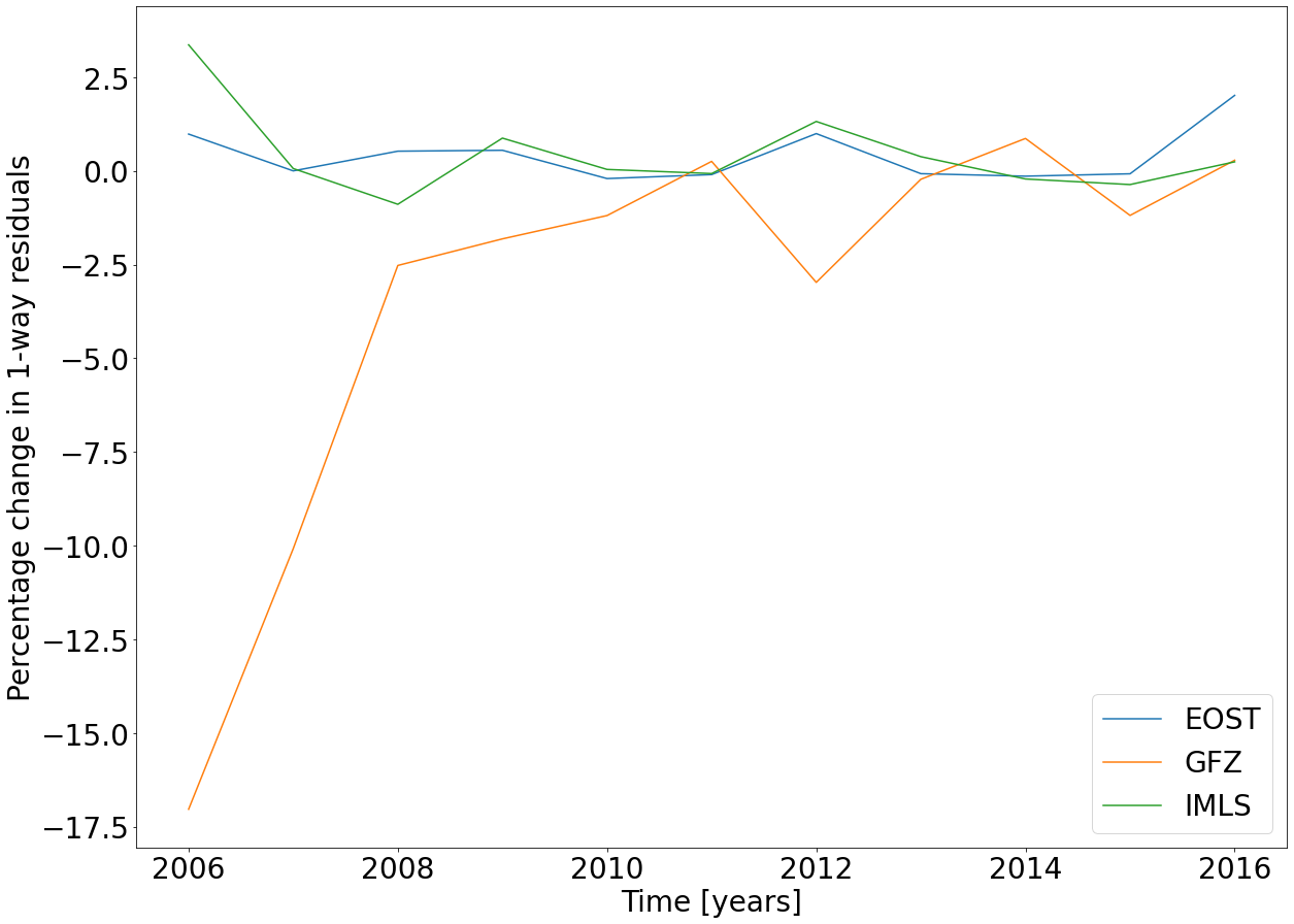
Figure 9: Percentage change in WRMS for the GFZ, IMLS, and EOST NTAL solutions compared to the standard solution for the APOLLO station.

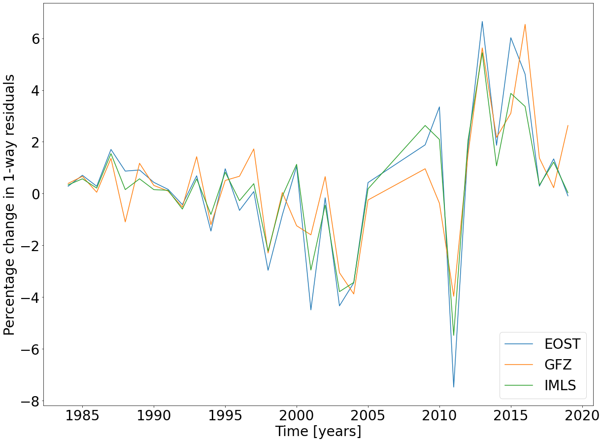
Figure 10: Percentage change in WRMS for the GFZ and IMLS NTOL solutions compared to the standard solution for the OCA station.

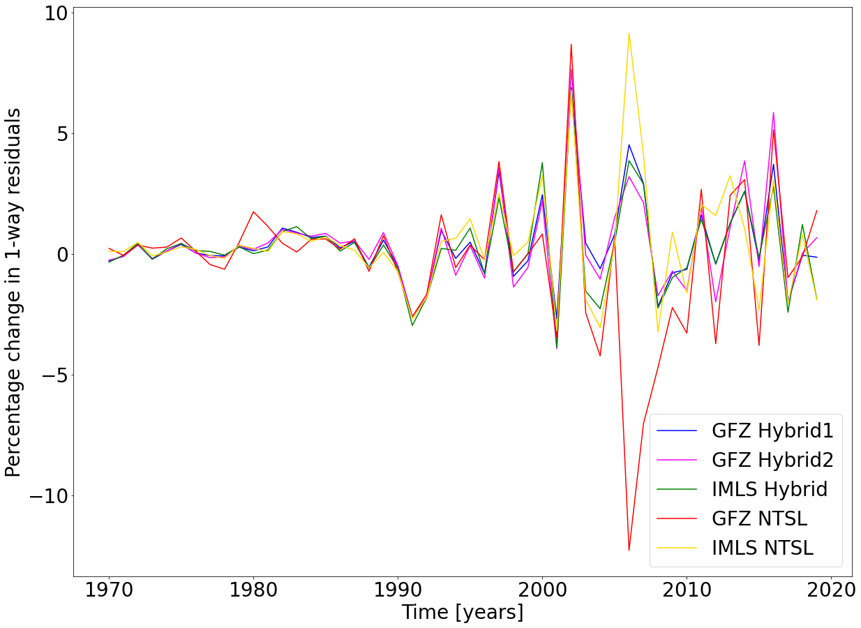
Figure 11: Percentage change in WRMS for the hybrid and NTSL solutions for GFZ and IMLS compared to the standard solution for all stations.

To ascertain if the HYDL at the APOLLO and McDonald stations is the only major difference between the datasets, we compute two hybrid solutions of GFZ and IMLS which add all loadings of both datasets (like NTSL) except HYDL and the APOLLO and McDonald stations. For GFZ, two hybrid versions, with and without including SLEL for all LLR stations, are named “Hybrid1” and “Hyrbid2”. The percentage change (compared to the standard solution) in the WRMS of the post-fit 1 way LLR residuals of the hybrid and NTSL solutions is shown in Figure 11. It can be seen that the hybrid solutions of GFZ Hybrid1 and IMLS show similar changes in percentages over the years, proving that only the HYDL at the APOLLO and McDonald stations casuses the significant differences between them. The GFZ Hybrid2 performs slightly better, showing that SLEL is an important addition to and a vital aspect of the GFZ datasets. By removing the HYDL at the APOLLO and McDonald stations, the high deterioration in 2006 (at APOLLO, see Figure 9) is avoided. However, it can also be seen that the IMLS NTSL solution outperforms all three of the hybrid solutions for 2006 and 2012, proving that HYDL at the APOLLO and McDonald stations plays an important role. The mean percentage change over the entire time series for the hybrid solutions are 0.41% for GFZ Hybrid1, 0.38% for GFZ Hybrid2 and 0.25% for IMLS.

3.2 LLR station positions

In LUNAR, the LLR station coordinates for epoch 2000.0, amongst other parameters, are adjusted. With this adjustment, the uncertainties of the station coordinates are obtained. The mean value of uncertainties (represented as 3-$\sigma$ values) of the coordinates of all six observatories used in LUNAR are given in Table 5 for the standard solution as well as for solutions using the NTL datasets. As the McDonald observatory conducted its LLR measurements for different times at three different locations which are very close to each other, namely McDonald, MLRS1, and MLRS2 (linked by local ties), they are analysed as one observatory in LUNAR.

Table 5: Mean values of 3-$\sigma$ uncertainties of LLR station coordinates (estimated for epoch 2000.0) obtained from LUNAR with the standard solution (Std), NTL solutions, and hybrid solutions.

Observatory	Dataset	GFZ	IMLS	EOST	Observatory	Dataset	GFZ	IMLS	EOST
		[mm]	[mm]	[mm]			[mm]	[mm]	[mm]
APOLLO	Std	6.65	6.65	6.65	LURE	Std	19.79	19.79	19.79
	NTAL	6.66	6.66	6.65		NTAL	19.82	19.82	19.79
	NTOL	6.66	6.66	-		NTOL	19.84	19.84	-
	HYDL	6.70	6.63	6.62		HYDL	19.94	19.73	19.71
	NTSL	6.71	6.63	6.61		NTSL	19.97	19.73	19.68
	Hybrid1	6.62	-	-		Hybrid1	19.72	-	-
	Hybrid2	6.63	6.63	-		Hybrid2	19.72	19.75	-
MLRS2∗	Std	9.68	9.68	9.68	OCA	Std	5.38	5.38	5.38
	NTAL	9.69	9.69	9.68		NTAL	5.39	5.39	5.38
	NTOL	9.70	9.70	-		NTOL	5.39	5.39	-
	HYDL	9.75	9.65	9.64		HYDL	5.42	5.37	5.36
	NTSL	9.77	9.65	9.62		NTSL	5.43	5.37	5.35
	Hybrid1	9.64	-	-		Hybrid1	5.36	-	-
	Hybrid2	9.65	9.66	-		Hybrid2	5.36	5.37	-
WLRS	Std	110.42	110.42	110.42	MLRO	Std	29.78	29.78	29.78
	NTAL	110.61	110.60	110.39		NTAL	29.83	29.83	29.77
	NTOL	110.68	110.69	-		NTOL	29.85	29.85	-
	HYDL	111.26	110.08	109.99		HYDL	30.01	29.69	29.66
	NTSL	111.43	110.11	109.8		NTSL	30.05	29.70	29.61
	Hybrid1	110.03	-	-		Hybrid1	29.67	-	-
	Hybrid2	110.05	110.17	-		Hybrid2	29.68	29.71	-

^∗: McDonald, MLRS1, and MLRS2 are linked by local ties and considered as one observatory for adjustment in LUNAR

For HYDL, the addition of the GFZ dataset leads to a deterioration for all stations (ranging between 0.72% and 0.77%) however, the addition of the IMLS and EOST datasets lead to an improvement for all stations (ranging between 0.19% and 0.31% and between 0.37% and 0.45%, respectively), also indicating that MERRA2 NWM suits LLR analysis better than LSDM. For NTAL, the addition of the GFZ and IMLS datasets show a slight deterioration (ranging between 0.10% and 0.19% from both datasets), whereas the addition of EOST shows either no change or a negligible improvement of up to 0.03%. For NTOL, addition of both GFZ and IMLS datasets show a deterioration (ranging between 0.15% and 0.25% from both datasets). When combining of all loadings from each dataset (represented as “NTSL” in the table), addition of GFZ shows a deterioration ranging between 0.90% and 0.93%, whereas the addition of IMLS and EOST show an improvement ranging between 0.19% and 0.31% and between 0.56% and 0.62%, respectively.

For the hybrid solutions (without HYDL at the APOLLO and McDonald stations), “Hyrbid1” and “Hyrbid2” stand for with and without SLEL for each station, and for IMLS “Hyrbid2” in the table represents the hybrid solution. The GFZ hybrid solutions show a minor improvement whereas the NTSL solutions show a deterioration, further stressing the importance of HYDL at the APOLLO and McDonald stations. Both the GFZ hybrid solutions perform show very similar results, indicating that SLEL does not have a significant effect on the solutions. For IMLS, the hybrid solution is either similar to, or worse than the NTSL solution, stressing on the importance of HYDL for the APOLLO and McDonald stations and therefore a better suitability of MERRA2 to LUNAR than LSDM.

3.3 Spectral analysis of LLR residuals

As the movement of atmospheric, oceanic, and surface water masses is seasonal in nature, it affects the signals obtained from time series of geodetic observations. Many authors, such as van Dam et al., (2012); Schuh et al., (2004); Dill and Dobslaw, (2013) and others, have pointed out the existence of an annual signal in all components of NTL, a semi-annual signal in mainly HYDL, and monthly and half-monthly signals in NTAL and NTOL. The strongest of these signals in all loadings is the annual signal. An addition of NTL in LLR should cause a corresponding effect in the time series of the LLR residuals.

The residuals from LLR contain many different signals, such as monthly, annual, et cetera. The investigation of signals with periods less than one month are difficult with LLR data, as the NPs normally do not cover the span of an entire month due to the lack of LLR observations during new and full Moon, constraining continuity of observations. LLR observations can be further constrained due lower elevations of the Moon, cloudy sky nights, et cetera. In this study, we focus on the annual signal obtained from the LLR time series, which may exist due to different reasons such as unmodelled geocenter motion in LUNAR, affect of asteroids on LLR analysis, et cetera.

The LLR observations are mostly taken at night, with more than one NP per night whenever possible. As the LLR observations can only be taken under certain restrictions (as mentioned above), they are temporally unevenly distributed. In this study, to perform a spectral analysis on this kind of a non-uniformly sampled data, the Lomb-Scargle (LS) periodogram is used. The magnitude of the LLR residuals in LS analysis is not a key factor as the output of the LS periodogram is dimensionless, which is always the case for the standard normalised periodograms.

To study the annual signal from the post-fit LLR residuals obtained from LUNAR, a suitable subset of the LLR time series (station wise) must be selected. VanderPlas, (2017) points out that to obtain a very clear distribution with LS periodogram, a high sampling rate and uniformity of data samples is needed. To best match this criteria, and to get a long enough timespan of residuals at one station, we identify two suitable subsets of time series from the post-fit residuals: from 15.06.2012 to 05.10.2018 at the OCA station (contains 5375 NPs), and 30.06.1994 to 25.01.2003 at MLRS2 (contains 2198 NPs). Figures 12 to 15 show the LS periodogram of the post-fit LLR residuals obtained at the OCA station for the standard solution and with solutions upon addition of NTL.

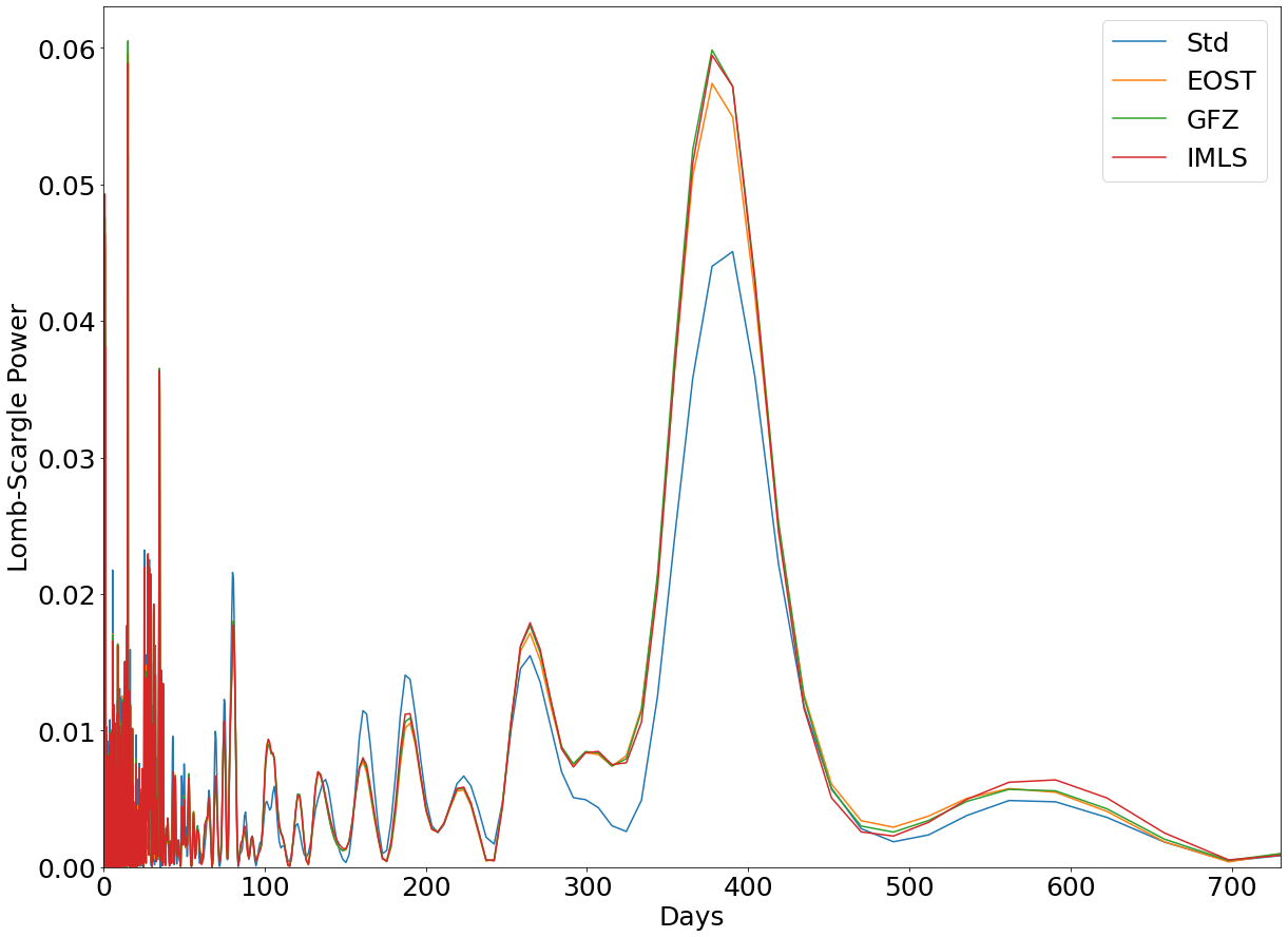
Figure 12: LS periodogram of post-fit LLR residuals obtained at the OCA station from 15.06.2012 to 05.10.2018 for the standard solution and the NTAL solution.

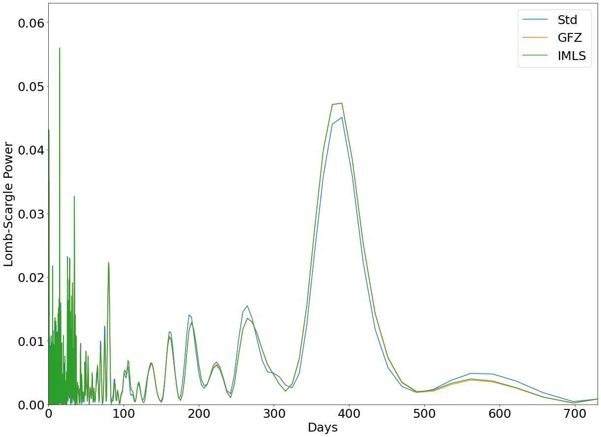
Figure 13: LS periodogram of post-fit LLR residuals obtained at the OCA station from 15.06.2012 to 05.10.2018 for the standard solution and the NTOL solution.

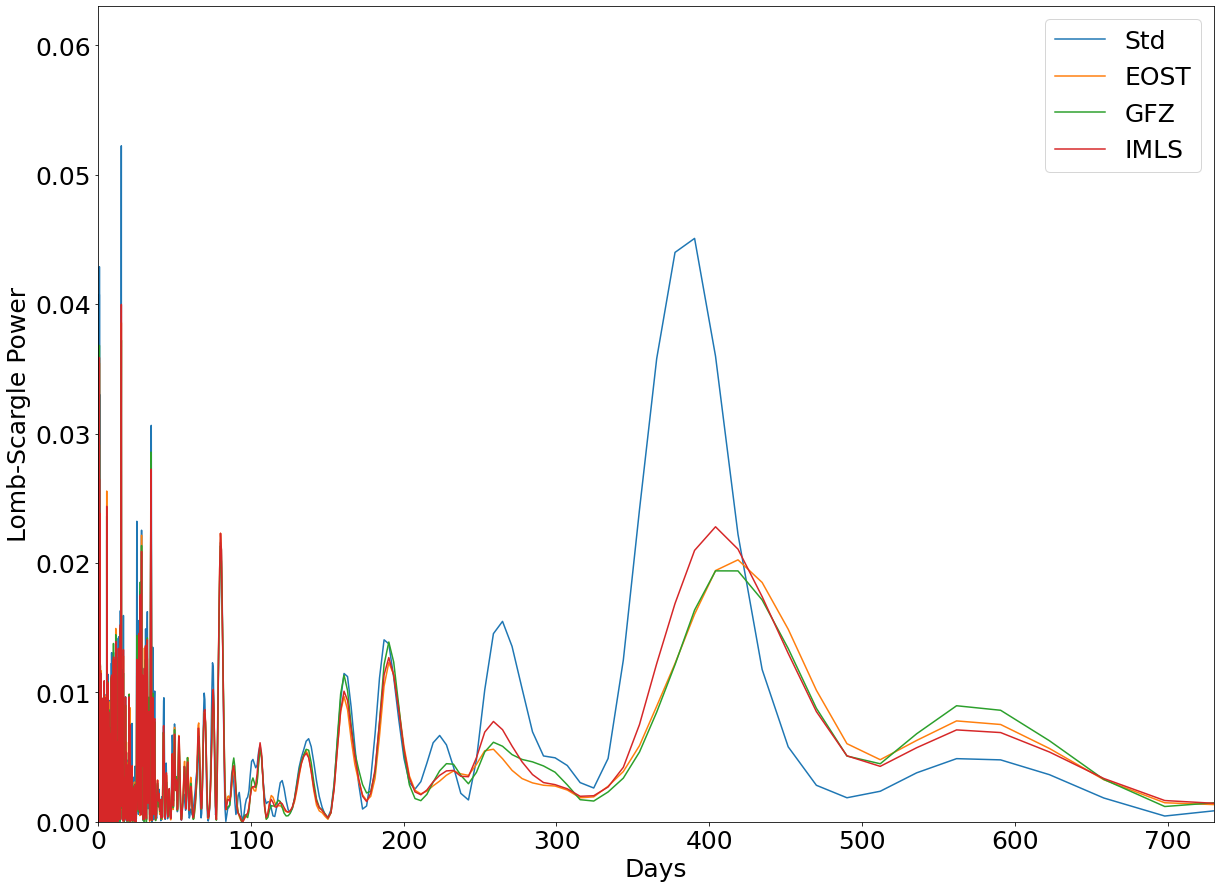
Figure 14: LS periodogram of post-fit LLR residuals obtained at the OCA station from 15.06.2012 to 05.10.2018 for the standard solution and the HYDL solution.

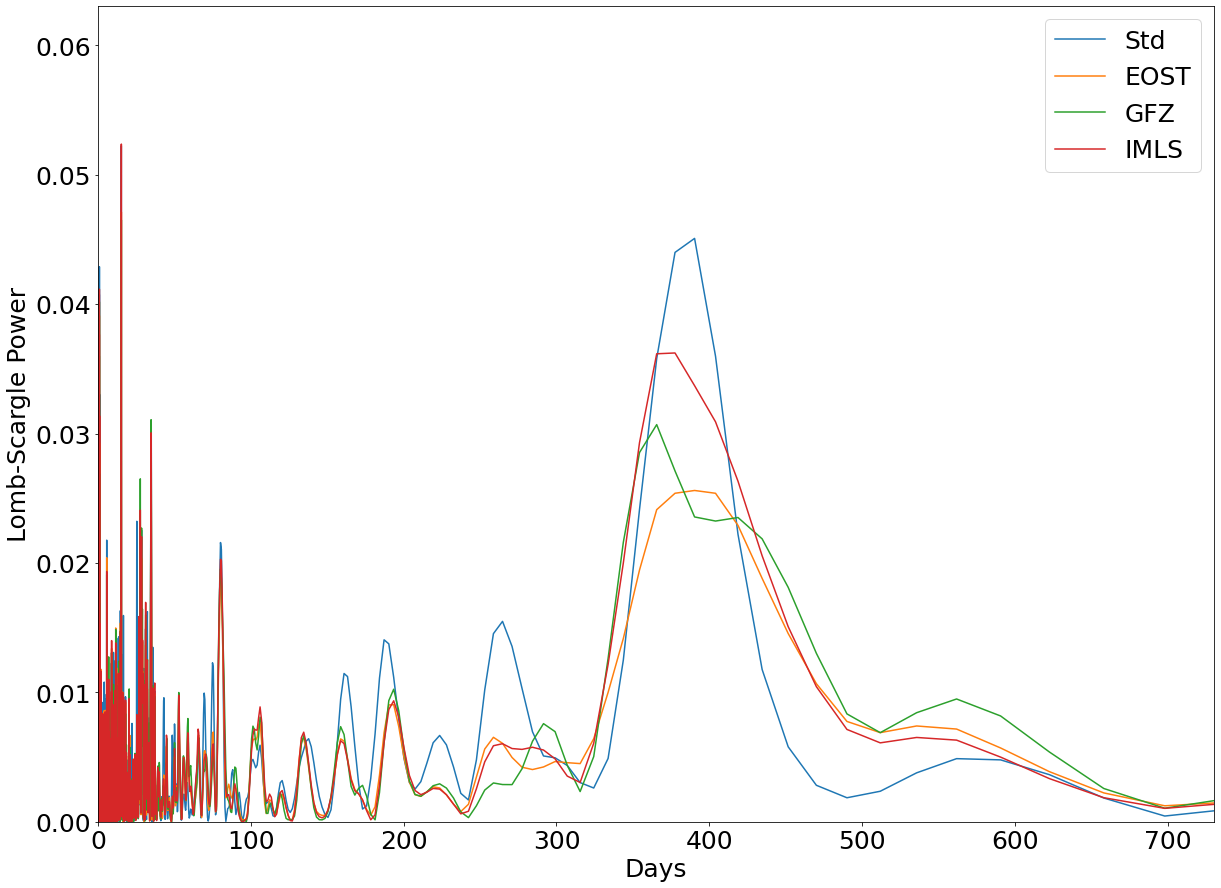
Figure 15: LS periodogram of post-fit LLR residuals obtained at the OCA station from 15.06.2012 to 05.10.2018 for the standard solution and the NTSL solution.

The annual signal observed from the time series is deviates from one year by several days because of the non-uniformity and low sample size of data (Zhang et al., , 2020). From Figure 12, it can be seen that when NTAL is added, the power at the annual period increases for all NTOL solutions. Here, all three NTOL solutions, EOST, GFZ, and IMLS, have similar powers, increasing compared to standard solution by 27.27%, 32.59%, and 31.93% respectively. An increase in power of signal at annual period when adding of NTAL is not uncommon, and was also pointed out by Petrov and Boy, (2004), Glomsda et al., (2020) and others.

With the addition of NTOL, the power at annual period is not significantly affected, showing an increase of 4.88% for both solutions in the LS power (see Figure 13), probably because of the small effect of NTOL at the OCA station.

When adding HYDL the power at the annual period decreases significantly for all solutions, as shown by Figure 15. The decrease for EOST solution is of 55.22%, for GFZ solution of 56.98%, and for IMLS solution of 49.45%. Glomsda et al., (2020) also observe a decrease in the annual period’s power when HYDL is added. As observed at the OCA station, the reduction in power due to addition of HYDL is stronger than the increase in powers due to addition of NTAL and NTOL, individually. Finally, when all loading components for all datasets are added together, shown by Figure 15, the annual signal shows a reduction in power (for EOST solution of 43.24%, for GFZ solution of 31.93%, and for IMLS solution of 19.74%), presumably due to HDYL’s role in the combined loading.

For the hybrid solutions at the OCA station (not shown), as expected, both values of the hybrid solutions are very similar to the NTSL solutions for the two datasets, as the loadings at the OCA station are not affected by the exclusion of HYDL at the APOLLO and McDonald stations.

Similar trends for all individual loadings and for the combined loading are noticed for the annual signal at MLRS2 in the subset time series from 30.06.1994 to 25.01.2003 (not shown). However the power of annual singal for all loadings and also for standard solution observed at MLRS2 is much smaller (LS power of 0.0089 for standard solution), probably because of fewer sample points (NPs) for a signal analysis using the LS periodogram. For the hybrid solutions, as expected, the power at annual signal increases, as the only component of NTL which leads to a reduction in the power at annual signal, i.e., HYDL is not added at McDonald stations.

4 Conclusions and further scope

In this study, the effect of NTL was applied as observation level corrections in LLR analysis to investigate its effect on the solutions obtained. The NTL was added as three different loading constituents for mass redistribution in atmosphere, oceans, and land water. The effect of NTL within LUNAR are analysed for data from three different data centres: EOST, GFZ, and IMLS due to the long enough time series of loadings available from these centres. Data from other providers is discussed to be in a range similar to the data used within this study. The impact of NTL on LLR analysis was discussed on solutions of WRMS of post-fit one-way LLR residuals, LLR station coordinates, and for the annual signal obtained from the time series of LLR residuals. The overall impact of NTL is determined to be small, however its addition would improve the LLR modelling and would be useful to achieve high accuracy from LLR analysis. Furthermore, NTL will play an important and more significant role when the accuracy of laser signals improves in future.

The impact on WRMS of post-fit one-way LLR residuals from LUNAR using data for each loading from all data providers is similar, except for HYDL which is similar for solutions from EOST and IMLS datasets, but differ for GFZ dataset. GFZ’s HYDL at the APOLLO and McDonald stations plays a critical role in deteriorating the results obtained upon the addition of HYDL from GFZ in LUNAR. This is further proved by the implementation of three hybrid solutions, which show the similarity of results if HYDL at the APOLLO and McDonald stations is not considered in solutions using the IMLS and GFZ datasets. Hence proving that for LLR analysis, the NWM MERRA2 leads to better results than LSDM. For the other stations, the results when adding of HYDL from GFZ are similar to addition of HYDL from either EOST or IMLS.

For the uncertainties of LLR station coordinates obtained via a Gauss-Markov adjustment performed within LUNAR, presented in this study as 3-$\sigma$ values, the addition of NTL shows only a small change. GFZ has the maximum influence, showing a deterioration ranging between 0.90% and 0.93% for all LLR stations. EOST (with both its loading components) and IMLS (with all three loading components) show an improvement ranging between 0.19% and 0.31% and between 0.56% and 0.62% for all LLR stations, respectively.

The most significant impact of addition of NTL is observed in the change of the power of the annual period in the post-fit LLR residuals at the OCA station. When HYDL is added, the power at annual period reduces by 55.22% for EOST, by 56.98% for GFZ, and by 49.45% for IMLS. Addition of NTAL and NTOL from all data provider shows an increase in the annual signal’s power at the OCA station. A combined solution of all loadings from data providers shows a decrease in the annual signal’s power at the OCA station for EOST of 43.24%, for GFZ of 31.93%, and for IMLS of 19.74%.

Based on this study, we conclude that addition of NTL makes a valid contribution in the LLR analysis, as it reduces systematic effects (even if small) which otherwise would smear over to other LLR parameters. The impact of each individual loading from the different data providers is similar, with the exception of HYDL from GFZ. Overall, the addition of NTL in LLR analysis is deemed to be beneficial to achieve smaller LLR residuals and reduced power of the annual signal in the time series of residuals. In a further study, we would discuss the EOP determination from LUNAR, using high accuracy data from OCA station, and estimate the impact of NTL on the EOP.

Data availability

LLR data is collected, archived, and distributed under the auspices of the International Laser Ranging Service (ILRS) (Pearlman et al., , 2002); and downloaded from the website. The IMLS non-tidal loading dataset is freely available on the IMLS website; and downloaded for the LLR observatories from the pre-computed time series of 1272 space geodesy sites. The GFZ non-tidal loading dataset is freely available on the ESMGFZ Product Repository page; and is downloaded using the script available at the website. The VMF non-tidal atmospheric loading dataset is freely available on the VMF website, and downloaded for LLR observatories from the pre-computed time series of SLR stations available at. The EOST non-tidal loading dataset is freely available on the EOST website, and downloaded for LLR observatories from the pre-computed time series of 7500 stations available at. The University of Luxumbourg non-tidal atmospheric loading dataset is freely available on the website, and downloaded using a modified version (edited to download loadings for LLR observatories) of the script available at.

References

- Altamimi et al., (2016) Altamimi, Z., Rebischung, P., Métivier, L., and Collilieux, X. (2016). Itrf2014: A new release of the international terrestrial reference frame modeling nonlinear station motions. Journal of Geophysical Research: Solid Earth, 121(8):6109–6131.
- Biskupek, (2015) Biskupek, L. (2015). Bestimmung der Erdorientierung mit Lunar Laser Ranging. PhD thesis, Leibniz University Hannover.
- Boy and Lyard, (2008) Boy, J.-P. and Lyard, F. (2008). High-frequency non-tidal ocean loading effects on surface gravity measurements. Geophysical Journal International, 175(1):35–45.
- Bury et al., (2019) Bury, G., Sośnica, K., and Zajdel, R. (2019). Impact of the atmospheric non-tidal pressure loading on global geodetic parameters based on satellite laser ranging to gnss. IEEE Transactions on Geoscience and Remote Sensing, 57(6):3574–3590.
- Dach et al., (2010) Dach, R., Böhm, J., Lutz, S., Steigenberger, P., and Beutler, G. (2010). Evaluation of the impact of atmospheric pressure loading modeling on GNSS data analysis. Journal of Geodesy.
- Dill and Dobslaw, (2013) Dill, R. and Dobslaw, H. (2013). Numerical simulations of global-scale high-resolution hydrological crustal deformations. JGR: Solid Earth, 118. doi:10.1002/jgrb.50353.
- Dill et al., (2018) Dill, R., Klemann, V., and Dobslaw, H. (2018). Relocation of river storage from global hydrological models to georeferenced river channels for improved load-induced surface displacements. Journal of Geophysical Research: Solid Earth, 123(8):7151–7164.
- Farrell, (1972) Farrell, W. E. (1972). Deformation of the earth by surface loads. Rev. Geophys. and Spac. Phys., 10(3):751–797. https://doi.org/10.1029/RG010i003p00761.
- Folkner et al., (2014) Folkner, W. M., Williams, J. G., Boggs, D. H., Park, R. S., and Kuchynka, P. (2014). The planetary and lunar ephemerides de430 and de431. IPN Progress Report 42-196.
- Gelaro et al., (2017) Gelaro, R., McCarty, W., Suárez, M. J., Todling, R., Molod, A., Takacs, L., Randles, C. A., Darmenov, A., Bosilovich, M. G., Reichle, R., Wargan, K., Coy, L., Cullather, R., Draper, C., Akella, S., Buchard, V., Conaty, A., da Silva, A. M., Gu, W., Kim, G.-K., Koster, R., Lucchesi, R., Merkova, D., Nielsen, J. E., Partyka, G., Pawson, S., Putman, W., Rienecker, M., Schubert, S. D., Sienkiewicz, M., and Zhao, B. (2017). The Modern-Era Retrospective Analysis for Research and Applications, Version 2 (MERRA-2). Journal of Climate - American Meteorological Society.
- Glomsda et al., (2020) Glomsda, M., Bloßfeld, M., Seitz, M., and Seitz, F. (2020). Benefits of non-tidal loading applied at distinct levels in VLBI analysis. Journal of Geodesy.
- Hersbach et al., (2018) Hersbach, H., de Rosnay, P., Bell, B., Schepers, D., Simmons, A., Soci, C., Abdalla, S., Balmaseda, M. A., Balsamo, G., Bechtold, P., Berrisford, P., Bidlot, J., de Boisséson, E., Bonavita, M., Browne, P., Buizza, R., Dahlgren, P., Dee, D., Dragani, R., Diamantakis, M., Flemming, J., Forbes, R., Geer, A., Haiden, T., Hólm, E., Haimberger, L., Hogan, R., Horányi, A., Janisková, M., Laloyaux, P., Lopez, P., Muñoz-Sabater, J., Peubey, C., Radu, R., Richardson, D., Thépaut, J.-N., Vitart, F., Yang, X., Zsótér, E., and Zuo, H. (2018). Operational global reanalysis: progress, future directions and synergies with nwp. Technical Report 27, European Centre for Medium Range Weather Forecasts, Shinfield Park, Reading, Berkshire RG2 9AX, England. https://doi.org/10.21957/tkic6g3wm.
- Hofmann, (2017) Hofmann, F. (2017). Lunar Laser Ranging –verbesserte Modellierung der Monddynamikund Schätzung relativistischer Parameter. PhD thesis, Leibniz University Hannover.
- Hofmann et al., (2018) Hofmann, F., Biskupek, L., and Müller, J. (2018). Contributions to reference systems from lunar laser ranging using the ife analysis model. Journal of Geodesy, 92:975–987. https://doi.org/10.1007/s00190-018-1109-3.
- Hofmann and Müller, (2018) Hofmann, F. and Müller, J. (2018). Relativistic tests with lunar laser ranging. Classical and Quantum Gravity, 35. doi:https://doi.org/10.1088/1361-6382/aa8f7a.
- Jungclaus et al., (2013) Jungclaus, J. H., Fischer, N., Haak, H., Lohmann, K., Marotzke, J., Matei, D., Mikolajewicz, U., Notz, D., and von Storch, J. S. (2013). Characteristics of the ocean simulations in the Max Planck Institute Ocean Model (MPIOM) the ocean component of the MPI‐Earth system model. Journal of Advances in Modeling Earth Systems.
- König et al., (2018) König, R., Fagiolini, E., Raimondo, J.-C., and Vei, M. (2018). A non-tidal atmospheric loading model: On its quality and impacts on orbit determination and c20 from slr. In Freymueller, J. T. and Sánchez, L., editors, International Symposium on Earth and Environmental Sciences for Future Generations, pages 189–194, Cham. Springer International Publishing.
- Murphy, (2013) Murphy, T. W. (2013). Lunar laser ranging: the millimeter challenge. Reports on Progress in Physics, 76. doi:10.1088/0034-4885/76/7/076901.
- Murphy et al., (2010) Murphy, T. W., Adelberger, E., Battat, J., Hoyle, C., Johnson, N., Mcmillan, R., Michelsen, E., Stubbs, C., and Swanson, H. (2010). Laser ranging to the lost lunokhod 1 reflector. Icarus, 211.
- Mémin et al., (2020) Mémin, A., Boy, J., and Santamaría-Gómez, A. (2020). Correcting GPS measurements for non-tidal loading. GPS Solutions.
- Mémin et al., (2014) Mémin, A., Watson, C., Haigh, I. D., MacPherson, L., and Tregoning, P. (2014). Non-linear motions of Australian geodetic stations induced by non-tidal ocean loading and the passage of tropical cyclones. Journal of Geodesy.
- Müller et al., (2014) Müller, J., Biskupek, L., Hofmann, F., and Mai, E. (2014). Lunar laser ranging and relativity. In Kopeikin, S., editor, Frontiers in relativistic celestial mechanics. Volume 2: Applications and experiments, volume 2, chapter 3, page 103–156. Walter de Gruyter, Berlin. ISBN: 3110345455, 9783110345452.
- Müller et al., (2009) Müller, J., Biskupek, L., Oberst, J., and Schreiber, U. (2009). Contribution of lunar laser ranging to realise geodetic reference systems. In Geodetic Reference Frames. International Association of Geodesy Symposia, volume 134, pages 55–59. Springer Berlin Heidelberg, Berlin, Heidelberg. https://doi.org/10.1007/978-3-642-00860-3-8.
- Müller et al., (2012) Müller, J., Hofmann, F., and Biskupek, L. (2012). Testing various facets of the equivalence principle using lunar laser ranging. Classical and Quantum Gravity - CLASS QUANTUM GRAVITY, 29.
- Müller et al., (2019) Müller, J., Murphy, T. W., Schreiber, U., Shelus, P. J., Torre, J. M., Williams, J. G., Boggs, D. H., Bouquillon, S., Bourgoin, A., and Hofmann, F. (2019). Lunar laser ranging: a tool for general relativity, lunar geophysics and earth science. Journal of Geodesy, 93:2195–2210. doi:https://doi.org/10.1007/s00190-019-01296-0.
- Nordman et al., (2015) Nordman, M., Virtanen, H., Nyberg, S., and Mäkinen, J. (2015). Non-tidal loading by the Baltic Sea: Comparison of modelled deformation with GNSS time series. GeoResJ.
- Oreiro et al., (2018) Oreiro, F. A., Wziontek, H., Fiore, M. M. E., D’Onofrio, E. E., and Brunini, C. (2018). Non-Tidal Ocean Loading Correction for the Argentinean-German Geodetic Observatory Using an Empirical Model of Storm Surge for the Río de la Plata. Pure and Applied Geophysics.
- Otsubo et al., (2004) Otsubo, T., Kubo-Oka, T., Gotoh, T., and Ichikawa, R. (2004). Atmospheric Loading Blue-Sky Effects on SLR Station Coordinates. In AGU Fall Meeting Abstracts, volume 2004, pages G31B–0793.
- Pavlov et al., (2016) Pavlov, D. A., Williams, J. G., and Suvorkin, V. V. (2016). Determining parameters of moon’s orbital and rotational motion from llr observations using grail and iers-recommended models. Celest Mech Dyn Astr, 126:61–88. https://doi.org/10.1007/s10569-016-9712-1.
- Pearlman et al., (2002) Pearlman, M. R., Degnan, J. J., and Bosworth, J. M. (2002). The international laser ranging service. Advances in Space Research. https://doi.org/10.1016/S0273-1177(02)00277-6.
- Petit and Luzum, (2010) Petit, G. and Luzum, B., editors (2010). IERS Conventions 2010. Number 36 in IERS Technical Note. Verlag des Bundesamtes für Kartographie und Geodäsie, Frankfurt am Main.
- Petrov, (2015) Petrov, L. (2015). The international mass loading service. http://arxiv.org/abs/1503.00191.
- Petrov and Boy, (2004) Petrov, L. and Boy, J. P. (2004). Study of the atmospheric pressure loading signal in very long baseline interferometry observations. JGR: Solid Earth. https://doi.org/10.1029/2003JB002500.
- Schuh et al., (2004) Schuh, H., Estermann, G., Crétaux, J.-F., Bergé-Nguyen, M., and van Dam, T. (2004). Investigation of hydrological and atmospheric loading by space geodetic techniques. In Hwang, C., Shum, C. K., and Li, J., editors, Satellite Altimetry for Geodesy, Geophysics and Oceanography, pages 123–132, Berlin, Heidelberg. Springer Berlin Heidelberg.
- Sośnica et al., (2013) Sośnica, K., Thaller, D., Dach, R., Jäggi, A., and G., B. (2013). Impact of loading displacements on SLR-derived parameters and on the consistency between GNSS and SLR results. Journal of Geodesy.
- Sun, (2017) Sun, Y. (2017). Estimating geocenter motion and changes in the Earth’s dynamic oblateness from GRACE and geophysical models. PhD thesis, TU Delft Physical and Space Geodesy. 10.4233/uuid:7fe64dde-7fb5-4392-8160-da6f7916dc6b.
- Thomas et al., (2020) Thomas, M., Dill, R., and Dobslaw, H. (2020). Sea-level loading product description. http://rz-vm115.gfz-potsdam.de:8080/repository/entry/show?entryid=0612018a-3ba4-44bc-86d9-1a429749fe4d, Last check: 18.05.2020.
- Tregoning and Watson, (2009) Tregoning, P. and Watson, C. (2009). Atmospheric effects and spurious signals in GPS analyses. JGR: Solid Earth.
- Tregoning and Watson, (2011) Tregoning, P. and Watson, C. (2011). Correction to “Atmospheric effects and spurious signals in GPS analyses”. JGR: Solid Earth.
- Tregoning et al., (2009) Tregoning, P., Watson, C., Ramillien, G., McQueen, H., and Zhang, J. (2009). Detecting hydrologic deformation using GRACE and GPS. Geophysical Research Letters, 36(15).
- van Dam et al., (1994) van Dam, T., Blewitt, G., and Heflin, M. (1994). Atmospheric pressure loading effects on Global Positioning System coordinate determinations. JGR: Solid Earth.
- van Dam et al., (2012) van Dam, T., Collilieux, X., Wuite, J., Altamimi, Z., and Ray, J. (2012). Nontidal ocean loading: amplitudes and potential effects in gps height time series. Journal of Geodesy, 86:1043–1057. doi:10.1007/s00190-012-0564-5.
- Van Dam et al., (2007) Van Dam, T., JM, W., and Lavallée, D. (2007). A comparison of annual vertical crustal displacements from gps and gravity recovery and climate experiment (grace) over europe. Journal of Geophysical Research, 112.
- Van Dam and Wahr, (1987) Van Dam, T. M. and Wahr, J. M. (1987). Displacements of the earth’s surface due to atmospheric loading: Effects on gravity and baseline measurements. Journal of Geophysical Research: Solid Earth, 92(B2):1281–1286.
- VanderPlas, (2017) VanderPlas, J. T. (2017). Understanding the lomb-scargle periodogram. The Astrophysical Journal Supplement Series, 236. doi:10.3847/1538-4365/aab766.
- Viswanathan et al., (2019) Viswanathan, V., Rambaux, N., andJ. Laskar, A. F., and Gastineau, M. (2019). Observational constraint on the radius and oblateness of the lunar core-mantle boundary. Geophysical Research Letters, 46:7295–7303. doi:https://doi.org/10.1029/2019GL082677.
- Williams, (2008) Williams, J. G. (2008). De421 lunar orbit, physical librations, and surface coordinates. Inteoffice Memorandum.
- Williams et al., (2013) Williams, J. G., Boggs, D. H., and Folkner, W. M. (2013). DE430 Lunar Orbit, Physical Librations, and Surface Coordinates. Technical report, Jet Propulsion Laboratory, California Institute of Technology, Pasadena, CA, USA. Interoffice memorandum, IOM 335-JW,DB,WF-20130722-016.
- Williams et al., (2006) Williams, J. G., Turyshev, S. G., Boggs, D. H., and Ratcliff, J. T. (2006). Lunar laser ranging science: Gravitational physics and lunar interior and geodesy. Advances in Space Research, 37:67–71. doi:https://doi.org/10.1016/j.asr.2005.05.013.
- Williams and Penna, (2011) Williams, S. D. P. and Penna, N. T. (2011). Non‐tidal ocean loading effects on geodetic GPS heights. JGR: Solid Earth.
- Wunsch and Stammer, (1997) Wunsch, C. and Stammer, D. (1997). Atmospheric loading and the oceanic “inverted barometer” effect. Reviews of Geophysics.
- Zhang et al., (2020) Zhang, M., Müller, J., and Biskupek, L. (2020). Test of the equivalence principle for galaxy’s dark matter by lunar laser ranging. Celestial Mechanics and Dynamical Astronomy, 132(4):25.