The natural frequencies of masonry beams

Abstract.

The present paper aims at analytically evaluating the natural frequencies of cracked slender masonry elements. The problem is dealt with in the framework of linear perturbation, and the small oscillations of the structure are studied under loaded conditions, after the equilibrium for permanent loads has been achieved. A masonry beam element made of no–tension (masonry–like) material is considered, and some explicit expressions of the beam’s fundamental frequency as a function of the external loads and the amplitude of imposed deformations are derived. The analytical results are validated via finite–element analysis.

1. Introduction

The measurement of ambient vibrations has become a standard procedure in Civil Engineering. In fact, these vibrations contain precious information on both the structural behaviour and the health status of buildings. Moreover, experimental frequencies and mode shapes can be introduced in model updating procedures [13] and allow estimating the mechanical properties and boundary conditions of such structures, while long–term measurements can help revealing the onset of structural damage, through damage detection procedures. In fact, modal properties are damage–sensitive features [2], [14], [24],

With regard to heritage masonry structures, the assumption of linear elasticity, which usually underlies the study of their ambient vibrations, may lead to errors. In fact, such structures are unable to withstand large tensile stresses and are usually affected by crack patterns. These nonlinear effects have in general a non–negligible influence on the structural stiffness and should not be disregarded in the analysis. The dynamic behaviour of these structures should be analyzed taking into account the existing cracks.

A great deal of effort has been devoted to numerically simulating the effects of damage on structural vibrations. With regard to masonry buildings, a common approach consists of simulating the cracks actually observed on the structure, by reducing the stiffness of the elements of the finite–element model which belong to the damaged parts [21], [23]. In [5] the dynamic properties of some masonry structures at different damage levels are investigated via the discrete element method. In [12] a linear–perturbation numerical procedure is presented, implemented in the NOSA–ITACA program [16], to take into account the presence of cracks in the calculation of a masonry structure’s dynamic properties. The procedure applies the constitutive equation of masonry–like materials [9], and the paper proves that the problem is governed by the global tangent stiffness matrix, used in place of the linear elastic one to evaluate the structure’s modal properties. Some example applications are shown in [20], where linear perturbation is carried out to model reinforcement operations on the Mogadouro tower in Portugal, and in [18], where the procedure is employed to reproduce the results of some laboratory tests conducted on a masonry arch subjected to settlements of one support.

Similar problems also arise in the study of the dynamic properties of prestressed concrete cracked elements; the dependence of such structures’ modal properties on the external loads and prestressing force level has long been debated, as shown in [1], [17], [19].

In the present paper, an analytical approach is presented to evaluate the natural frequencies of masonry beams. The small oscillations of such structures are studied under loaded conditions, after the equilibrium for permanent loads has been achieved. An explicit expressions of the beam’s fundamental frequency as a function of the external loads and initial deformations is derived, by using a constitutive relationship between the generalized deformation $\chi$ and the generalized stresses $N$ and $M$ acting on the beam’s sections.

The simple case presented in the paper turns out to be of interest, since at the best of the Author’s knowledge the literature do not furnish yet explicit expressions to estimate the effects of cracking on the natural frequencies of masonry structures.

The paper is organized as follows: in Section 2 the problem is introduced. Section 3 briefly recalls the constitutive equation of masonry–like beams and in Section 4 some example applications are presented. Finally, Section 5 is devoted to testing of the analytical results via finite–element analysis.

2. Small oscillations of a loaded masonry beam

Let us consider a rectilinear beam with length $l$ and rectangular cross section with height $h$ and width $b$, subjected along its axis to a constant axial force $N$. Let us denote by $E$ and $\rho$ the Young’s modulus and the density of the material, respectively, and by $J=bh^{3}/12$ the moment of inertia of the beam’s cross section. Let $x$ be the abscissa along the beam’s axis and $t$ the time.

The curvature of the beam is denoted by $\chi$ and, under the Euler–Bernoulli hypothesis, the bending moment $M(\chi):R\to R$ is a continuous differentiable function, whose second derivative is assumed to be piecewise continuous.

We assume the effects of both the shear strain and the rotary inertia to be negligible. Moreover, we limit ourselves to considering situations in which the transverse displacement $\phi(x,t)$ and its derivative $\phi(x,t)_{x}$ are small, so that we can neglect the effects of the axial force on the dynamic equilibrium of the beam and write

$$\chi(x,t)=-\phi_{x,x}(x,t).$$ (2-1)

If we introduce function

$$f(\chi)=\frac{M(\chi)}{\rho\,b\,h},$$ (2-2)

the motion of the beam is expressed by

$$\phi_{t,t}-(f(\chi))_{x,x}=q(x,t),$$ (2-3)

where

$$q(x,t)=\frac{p(x,t)}{\rho\,b\,h}$$ (2-4)

and $p(x,t)$ is the transverse load per unit length.

Let us consider, at $t=0$, a load $\mathrm{bar}q(x)$ inducing in the beam an initial deformation $\mathrm{bar}\phi(x)$ and curvature change $\mathrm{bar}\chi(x)$. The beam reaches equilibrium under the load $\mathrm{bar}q$, and thus

$$-f(\mathrm{bar}\chi)_{x,x}=\mathrm{bar}q(x).$$ (2-5)

We are interested in studying the small oscillations $\delta\phi$ of the beam around $\mathrm{bar}\phi$.

$$\delta\phi_{t,t}-\left(\frac{\partial f}{\partial\chi}\Bigg{|}_{\mathrm{bar}\chi}\delta\chi\right)_{x,x}=0,$$ (2-6)

where we use the approximation

$$f(\mathrm{bar}\chi+\delta\chi)\simeq f(\mathrm{bar}\chi)+\frac{\partial f}{\partial\chi}\Bigg{|}_{\mathrm{bar}\chi}\delta\chi.$$ (2-7)

In case of a simply supported beam, since we limit ourselves to studying the fundamental frequency of the beam, we can approximate the small oscillations $\delta\phi$ as follows:

$$\delta\phi\simeq\delta a\sin\left(\frac{\pi}{L}x\right)u(t),$$ (2-8)

where $\delta a>0$ represents the amplitude of the beam’s oscillation around $\mathrm{bar}\phi$. In view of (2-8), (2-6) becomes

$$\sin\left(\frac{\pi}{L}x\right)\ddot{u}-\left(\frac{\pi}{L}\right)^{2}\left(\frac{\partial f}{\partial\chi}\Bigg{|}_{\mathrm{bar}\chi}\sin{\left(\frac{\pi}{L}x\right)}\right)_{x,x}u=0.$$ (2-9)

Let us now use the Galerkin method, multiply (2-9) by $\sin{\left(\frac{\pi}{L}x\right)}$ and integrate over the beam’s length. The first member of the equation becomes:

$$\ddot{u}\int_{0}^{L}\sin\left(\frac{\pi}{L}x\right)^{2}dx-\frac{\pi^{2}}{L^{2}}\left(\int_{0}^{L}\sin\left(\frac{\pi}{L}x\right)\left(\frac{\partial f}{\partial\chi}\Bigg{|}_{\mathrm{bar}\chi}\sin{\left(\frac{\pi}{L}x\right)}\right)_{x,x}dx\right)u=$$

$$=\frac{L}{2}\ddot{u}-\frac{\pi^{2}}{L^{2}}\left(\sin{\left(\frac{\pi}{L}x\right)\left(\frac{\partial f}{\partial\chi}\Big{|}_{\mathrm{bar}\chi}\sin{\left(\frac{\pi}{L}x\right)}\right)_{x}}\Bigg{|}_{0}^{L}-\int_{0}^{L}\frac{\pi}{L}\cos\left(\frac{\pi}{L}x\right)\left(\frac{\partial f}{\partial\chi}\Bigg{|}_{\mathrm{bar}\chi}\sin{\left(\frac{\pi}{L}x\right)}\right)_{x}dx\right)u=$$

$$=\frac{L}{2}\ddot{u}+\frac{\pi^{3}}{L^{3}}\left(\int_{0}^{L}\cos\left(\frac{\pi}{L}x\right)\left(\frac{\partial f}{\partial\chi}\Bigg{|}_{\mathrm{bar}\chi}\sin{\left(\frac{\pi}{L}x\right)}\right)_{x}dx\right)u=$$

$$=\frac{L}{2}\ddot{u}+\frac{\pi^{3}}{L^{3}}\left(\cos{\left(\frac{\pi}{L}x\right)\frac{\partial f}{\partial\chi}\Big{|}_{\mathrm{bar}\chi}\sin{\left(\frac{\pi}{L}x\right)}}\Bigg{|}_{0}^{L}+\frac{\pi}{L}\int_{0}^{L}\sin^{2}\left(\frac{\pi}{L}x\right)\frac{\partial f}{\partial\chi}\Bigg{|}_{\mathrm{bar}\chi}dx\right)u,$$

where we used the boundary conditions $\sin{\left(\frac{\pi}{L}x\right)}\Bigg{|}_{0}^{L}=0$. Thus, equation (2-9) becomes

$$\ddot{u}+\frac{2\pi^{4}}{L^{5}}\left(\int_{0}^{L}\sin^{2}\left(\frac{\pi}{L}x\right)\frac{\partial f}{\partial\chi}\Bigg{|}_{\mathrm{bar}\chi}dx\right)u=0.$$ (2-10)

The fundamental frequency can be directly obtained from equation (2-10), once the constitutive equation $f(\chi)$ is given.

Figure 1. The beam model.

3. A constitutive equation for masonry–like beams

In this section we briefly recall a simple constitutive equation for one–dimensional masonry–like elements with rectangular cross section. Despite its simplicity, this constitutive equation effectively describes the mechanical behaviour of a masonry beam subjected to axial force and bending moment. The beam’s cross section is fully compressed since the vertical load falls inside the central nucleus of inertia, and reaches the limit elastic behaviour when the vertical load acts on the perimeter. Many authors have made use of this simplified equation to find analytical and numerical solutions to the static and the dynamic behaviour of masonry beams and arches (some examples can be found in [3],[7], [8],[15],[25]). In [10] and [11] some explicit approximate solutions are proposed for modelling the free and forced oscillations of masonry beams.

Under the classical hypothesis of Euler–Bernoulli and providing that the axial force $N$ along the beam’s axis is known, infinite compressive strength is allowed, and the material is unable to withstand tensile stresses, function $f(\chi)$ becomes:

$$f(\chi)=\begin{cases}\quad c^{2}\chi\quad&\text{for $\left|\chi\right|\leq\alpha$},\\ \quad c^{2}\alpha\operatorname{Sign}(\chi)(3-2\sqrt{\frac{\alpha}{{\left|\chi\right|}}})\quad&\text{for}\left|\chi\right|>\alpha,\end{cases}$$ (3-1)

where

$$\alpha=-\frac{2N}{Ebh^{2}}$$ (3-2)

is the curvature corresponding to the elastic limit and $c^{2}=\frac{EJ}{\rho bh}$ is the elastic constant of the beam.

Function (3-1) is plotted in Figure 2. In the nonlinear region, for $\left|\chi\right|>\alpha$, increasing values of $\chi$ correspond to a rapid decrease in the section’s stiffness, and the bending moment tends toward its limit value $\left|Nh/2\right|$. Moreover, $M(\chi)$ is continuous with its first derivative, while the second derivative undergoes a jump at $\left|\chi\right|=\alpha$.

Figure 2. The constitutive equation $M-\chi$ for a rectangular section with infinite compressive strength and zero tensile stress.

Equation (3-1) is used in the following in conjunction with (2-10) to explicitly evaluate the fundamental frequency of masonry beams subjected to different loading conditions. The first derivative of $f$ with respect to $\chi$, which appears in (2-10), is:

$$f^{\prime}(\chi)=\begin{cases}\quad c^{2}\quad&\text{for $\left|\chi\right|\leq\alpha$},\\ \quad c^{2}\sqrt{\frac{\alpha^{3}}{{\left|\chi\right|}^{3}}}\quad&\text{for}\left|\chi\right|>\alpha.\end{cases}$$ (3-3)

4. Example applications

4A. Case 1: constant curvature

Let us consider the case of a masonry beam in an initial deformed shape with constant curvature $\mathrm{bar}\chi$. This is the simple, but meaningful case of a beam subjected to a vertical load acting with constant eccentricity $e$ along the axis. In this case, the bending moment acting on the beam assumes the constant value

$$M=N\cdot e,$$ (4-1)

and nonlinear behaviour of the structure is attained for the eccentricity

$$\left|e\right|=\frac{h}{6}.$$ (4-2)

Thus, from (2-10) and (3-3) the fundamental frequency $\omega$ of the beam (in radians per second) is:

$$\omega^{2}=\frac{\pi^{4}}{L^{4}}\,c^{2}=\omega_{el}^{2}\quad \text{for}\left|\mathrm{bar}\chi\right|\leq\alpha,$$ (4-3)

$$\omega^{2}=\frac{2\pi^{4}c^{2}}{L^{5}}\int_{0}^{L}\sin^{2}\left(\frac{\pi x}{L}\right)\sqrt{\frac{\alpha^{3}}{\left|\mathrm{bar}\chi\right|^{3}}}\,dx\quad \text{for}\left|\mathrm{bar}\chi\right|>\alpha,$$ (4-4)

and $\mathrm{bar}\chi$, given the bending moment (4-1) , can be deduced from (3-1)

$$\left|\mathrm{bar}\chi\right|=\frac{4\,\alpha^{3}\,c^{4}}{(\left|f\right|-3\,\alpha\,c^{2})^{2}}.$$ (4-5)

Equation (4-3) coincides with the fundamental frequency of a linear elastic beam [6] and can be deduced by means of (2-10), per $\chi=\alpha$ . When the eccentricity reaches the border of the section, $\left|e\right|=h/2$, the frequency of the beam tends to zero.

It is worth noting that the value of the linearized frequency (4-4) does not depend on the normal force $N$, but only on the eccentricity $e$. In fact, using (4-1) and (4-5), after simple calculations, the frequency assumes the following expression:

$$\omega=\frac{\pi^{2}}{L^{2}}\,c=\omega_{el}\quad \text{for}\left|e\right|\leq\frac{1}{6},$$ (4-6)

$$\omega=\frac{3}{4}\,\frac{\pi^{2}c}{L^{2}}\sqrt{6\left(1-2\frac{\left|e\right|}{h}\right)^{3}}=\frac{3}{4}\,\omega_{el}\sqrt{6\left(1-2\frac{\left|e\right|}{h}\right)^{3}}\quad \text{for}\frac{1}{6}<\left|e\right|\leq\frac{1}{2}.$$ (4-7)

Equations (4-6) and (4-7) are plotted in Figure 3.

Figure 3. Case 1: ratio $\omega el/\omega$ vs. eccentricity $|e|$ of the axial load $N$.

4B. Case 2: uniform transverse load

Let us consider the case of a beam subjected to a uniform transverse load $p$ and axial force $N$.

Figure 4. Case 2: uniform transverse load.

The beam enters the nonlinear field when $p$ reaches the value

$$\mathrm{bar}p=\frac{4\left|N\right|\,h}{3\,L^{2}}.$$ (4-8)

For greater values of the transverse load, the beam’s axis can be divided into three regions: the central part of the beam is in the nonlinear field, while two lateral regions, symmetric with respect to the midsection, still exhibit linear behaviour (see Figure 4). Let us denote by $x_{0}$ the abscissa of the beam’s section with curvature $\chi=\alpha$, $0\leq x_{0}\leq L/2$. Function $x_{0}$ can be easily deduced:

$$x_{0}=\begin{cases}\quad\frac{L}{2}\quad&\text{for $p<\mathrm{bar}p$},\\ \quad\frac{L}{2}-\frac{L}{2}\sqrt{1-\frac{\mathrm{bar}p}{p}}\quad&\text{for $p\geq\mathrm{bar}p$}.\end{cases}$$ (4-9)

In view of (2-10), the expression for the fundamental frequency becomes, for $p\geq\mathrm{bar}p$

$$\omega^{2}=\frac{4\pi^{4}c^{2}}{L^{5}}\left(\int_{0}^{x_{0}}\sin^{2}\left(\frac{\pi x}{L}\right)\,dx+\int_{x_{0}}^{L/2}\sin^{2}\left(\frac{\pi x}{L}\right)\sqrt{\frac{\alpha^{3}}{\left|\mathrm{bar}\chi\right|^{3}}}\,dx\right),$$ (4-10)

with $\left|\mathrm{bar}\chi\right|$ given by (4-5). After simple calculations, equation (4-10) can be expressed in the following form

$$\omega^{2}=4\omega_{el}^{2}\left(\int_{0}^{x_{0}/L}\sin^{2}(\pi\,y)\,dy+8\int_{x_{0}/L}^{1/2}\sin^{2}(\pi\,y)\left|\frac{p}{\mathrm{bar}p}(y-y^{2})-\frac{3}{4}\right|^{3}\,dy\right),$$ (4-11)

with $y=x/L$. Thus, ratio $\omega/\omega_{el}$, shown in Figure 5, turns out to be dependent only on the ratio $p/\mathrm{bar}p$.

The mid–section of the beam reaches the limit bending moment for the transverse load

$$\mathrm{bar}{\mathrm{bar}p}=\frac{4\left|N\right|\,h}{L^{2}}=3\,\mathrm{bar}p.$$ (4-12)

Accordingly, abscissa $x_{0}$ attains the value

$$x_{0}=\frac{L}{2}-\frac{L}{\sqrt{6}},$$ (4-13)

which is independent of the transverse load and the normal force acting and corresponds to about one tenth of the beam’s total length. In this case, equation (4-11) reduces to

$$\left(\omega/\omega_{el}\right)^{2}=4\left(\int_{0}^{\frac{1}{2}-\frac{1}{\sqrt{6}}}\sin^{2}(\pi y)\,dy+8\int_{\frac{1}{2}-\frac{1}{\sqrt{6}}}^{1/2}\sin^{2}(\pi y)\left|3\,(y-y^{2})-\frac{3}{4}\right|^{3}\,dy\right)\simeq 0.05.$$ (4-14)

Figure 5. Case 2: ratio $(\omega el/\omega)^{2}$ vs. ratio $p/\mathrm{bar}p$.

4C. Case 3: Initial deformed shape

In this last case, let us impose on the beam an initial deformation defined by the following equation:

$$\mathrm{bar}\phi(x)=A\,\sin\left(\frac{\pi x}{L}\right)$$ (4-15)

with $A\geq 0$. Accordingly, curvature $\mathrm{bar}\chi$ assumes the value

$$\mathrm{bar}\chi(x)=\frac{A\pi^{2}}{L^{2}}\sin\left(\frac{\pi x}{L}\right),$$ (4-16)

and, setting $\mathrm{bar}\chi=\alpha$, abscissa $x_{0}$ becomes

$$x_{0}=\frac{L}{\pi}\arcsin\left(\frac{\alpha L^{2}}{A\pi^{2}}\right).$$ (4-17)

Function $x_{0}$ is $L/2$ for

$$A_{m}=\alpha L^{2}/\pi^{2},$$ (4-18)

and tends to zero for $A\to\infty$.

In this case, equations (2-10) and (3-3) yield:

$$\begin{split}\omega^{2}=&\frac{2\pi^{4}c^{2}}{L^{5}}\left(2\int_{0}^{x_{0}}\sin^{2}\left(\frac{\pi x}{L}\right)\,dx+\int_{x_{0}}^{L-x_{0}}\sin^{2}\left(\frac{\pi x}{L}\right)\sqrt{\frac{\alpha^{3}L^{6}}{A^{3}\pi^{6}\sin\left(\frac{\pi x}{L}\right)^{3}}}\,dx\right)=\\ =&\frac{2\pi^{4}c^{2}}{L^{5}}\left(x_{0}-\frac{L^{3}\alpha}{A\pi^{3}}\sqrt{1-\frac{L^{4}\alpha^{2}}{A^{2}\pi^{4}}}+\frac{L^{3}\alpha}{A\pi^{3}}\int_{x_{0}}^{L-x_{0}}\sqrt{\frac{\alpha}{A}\sin\left(\frac{\pi x}{L}\right)}\,dx\right)=\\ =&2\,\omega_{el}^{2}\left(\frac{x_{0}}{L}-\frac{A_{m}}{\pi A}\sqrt{1-\left(\frac{A_{m}}{A}\right)^{2}}+\int_{\frac{x_{0}}{L}}^{1-\frac{x_{0}}{L}}\sqrt{\left(\frac{A_{m}}{A}\right)^{3}\sin(\pi y)}\,dy\right),\end{split}$$ (4-19)

where the first two terms regard the unfractured part of the beam, while the third is for the fractured part. For $A=A_{m}$ frequency (4-19) reduces to the linear elastic value $\omega_{el}$, while for $A\to\infty$ the frequency tends to zero. Function $x_{0}/L$ depends solely on the variable $A_{m}/A$. Thus, as for the previous cases, expression (4-19) can be expressed in the non–dimensional form shown in Figure 6.

Figure 6. Ratio $(\omega el/\omega)^{2}$ vs. ratio $A/A_{m}$.

5. Numerical solutions

The analytical solutions have been tested against finite element analysis. To this end, we adopt a conforming beam element equipped with cubic polynomial shape functions (Hermite polynomials), thereby guaranteeing continuity of both the transverse displacements and rotations of the beam’s axis [4]. Accordingly, the beam element has two degrees of freedom for each node: one for the beam’s transverse displacement $\phi$, the other associated to its derivative $\phi_{x}$.

The first application of this element to masonry–like beams is reported on in [15], [22], where the element is described in detail. Here the main ingredients of the calculation are briefly recalled. The core of the analysis is calculation of the element tangent stiffness matrix, which for constitutive equation (3-1) takes the explicit form

$$\mathbf{K}^{e}_{T}=\frac{EJ}{c^{2}}\int_{e}\bm{\Psi}^{\prime\prime}\bm{\Psi}^{\prime\prime\text{T}}\,f^{\prime}\,d\xi$$ (5-1)

where $\bm{\Psi}$ is the vector of the shape functions, $f^{\prime}(\chi)$ is given by equations (3-3), and relation (2-1) holds true. The vector of the element’s internal forces is

$$\mathbf{f}_{i}^{\,e}=\frac{EJ}{c^{2}}\int_{e}\bm{\Psi}^{\prime\prime}\,f\,d\xi,$$ (5-2)

where $f$ is given by (3-1), while the vector of the external loads acting on the element and the mass matrix of the element assume the usual expressions

$$\mathbf{f}_{e}^{\,e}=\int_{e}\bm{\Psi}p\,d\xi,$$ (5-3)

$$\mathbf{M}^{e}=\rho bh\int_{e}\bm{\Psi}\,\bm{\Psi}^{T}d\xi.$$ (5-4)

The numerical procedure adopted here follows the method shown in [12] and is known as linear perturbation. This method consists of the following steps:

Step 1. Model the structure via finite elements.

Step 2. Apply external loads and solve the nonlinear equilibrium problem through an iterative scheme. Extract the tangent stiffness matrix calculated in the last iteration before convergence.

Step 3. Perform a modal analysis about the equilibrium solution, using the tangent stiffness matrix in place of the linear elastic one.

Herein the finite element (5-1)–(5-4), implemented in the Mathematica environment, is used to model the masonry beam. For each load case, the tangent stiffness matrix is calculated via a Newton–Raphson scheme, and the corresponding value of the fundamental frequency is evaluated. This value is then compared to the analytical solutions reported in Section 4.

The numerical procedure is applied to a masonry–like beam–column with the following geometric characteristics:

$$\begin{split}&L=$6\text{\,}\mathrm{m}$,\\ &h=$0.4\text{\,}\mathrm{m}$,\\ &b=$1\text{\,}\mathrm{m}$,\\ &\rho=$1800\text{\,}\mathrm{k}\mathrm{g}\mathrm{/}\mathrm{m}^{3}$,\\ &E=$3\cdot 10^{9}\text{\,}\mathrm{Pa}$,\\ \end{split}$$ (5-5)

The beam is simply supported at the ends and discretized into $30$ elements (different numbers of elements have been also tested to check software performance). The example applications presented regard the three cases presented in Section 4.

5A. Case 1: constant curvature

Beam (5-5) is subjected to increasing values of the eccentricity. The normal force acting on the model is $N=$-500000\text{\,}\mathrm{N}$$. Different tests, not reported on here, have been performed to check the influence of the normal force on the beam’s fundamental frequency given eccentricity $e$: the numerical value of the frequency turned out to be independent of the normal force, as predicted by the analytical solution.

Figure 7 shows the beam’s fundamental frequency $f_{fun}$ versus the eccentricity $e$ of the normal force. The analytical solution (4-7), (4-6) is plotted as a continuous line, while boxes are for the finite element simulation.

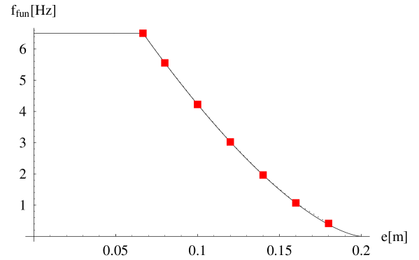
Figure 7. Fundamental frequency $\text{f}_{\text{fun}}$ vs. the eccentricity $e$ of the normal force. Analytical solution in continuous line, while boxes represent the FE simulation.

5B. Case 2: uniform transverse load

Beam (5-5) is subjected to a transverse load $p$ of increasing amplitude, with a normal force $N$ acting along the beam. Different values of $N$ are tested. The beam’s fundamental frequency is shown in Figure 8, where lines represent the analytical solution (4-10), while boxes represent the results of the finite element analysis.

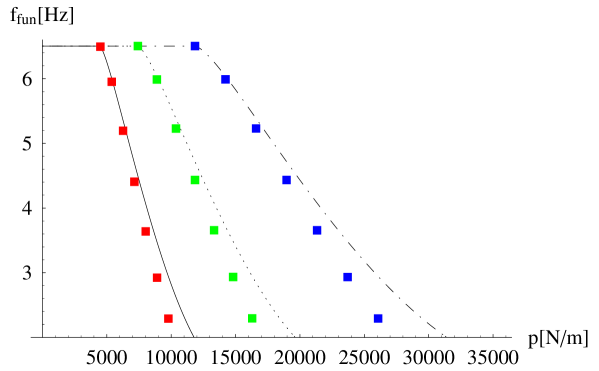
Figure 8. Fundamental frequency $\text{f}_{\text{fun}}$ vs. transverse load $p$. Continuous line: $N=$-300000\text{\,}\mathrm{N}$$. Dotted line: $N=$-500000\text{\,}\mathrm{N}$$. Dash–dotted: $N=$-800000\text{\,}\mathrm{N}$$. Boxes represent the FE simulation.

5C. Case 3: initial deformed shape

Beam (5-5) is in an initial deformed shape defined by equation (4-15). Increasing values of the maximum amplitude $A$ are evaluated for different values of the normal force $N$ acting along the beam. The beam’s fundamental frequency is shown in Figure 9, where lines represent the analytical solution (4-19), while boxes represent the results of the finite element analyses.

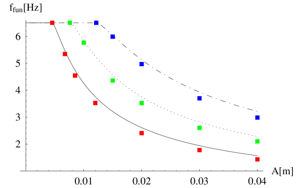
Figure 9. Fundamental frequency $\text{f}_{\text{fun}}$ vs. the amplitude $A$ of the initial displacement. Continuous line: $N=$-300000\text{\,}\mathrm{N}$$. Dotted line: $N=$-500000\text{\,}\mathrm{N}$$. Dash–dotted: $N=$-800000\text{\,}\mathrm{N}$$. Boxes represent the FE simulation.

Conclusions

An analytical approach to determine the fundamental frequency of masonry beam–columns in the presence of cracks has been presented. The study has been carried out under the hypothesis of masonry–like material. Some explicit expressions have been obtained, with the frequency depending on the external loads acting or the initial deformation imposed on the beam. The analytical method has been validated via finite–element analysis, and such a comparison reveals the good agreement found between between the numerical and analytical results.

References

- [1] H. Abdel-Jaber and B. Glisic. Monitoring of prestressing forces in prestressed concrete structures – An overview. Structural Control and Health Monitoring 2019; 26:e2374.
- [2] Agarwali S, Chaudhuri SR. Damage detection in large structures using mode shapes and its derivatives. International Journal of Research in Engineering and Technology 2015; 4, Special Issue 13.
- [3] R. Barsotti and S. Bennati. A simple and effective nonlinear elastic one-dimensional model for the structural analysis of masonry arches. Meccanica 2018; 53: 1899-1915.
- [4] E.B Becker, G.F. Carey, J.T. Oden. Finite Elements: An Introduction Prentice–Hall, Inc., New Jersey, 1981.
- [5] Bui TT, Limam A, Bui QB. Characterisation of vibration and damage in masonry structures: experimental and numerical analysis. European Journal of Environmental and Civil Engineering 2014; 18(10), 1118–1129.
- [6] R.W. Clough, J. Penzien. Dynamics of Structures Mc–Graw Hill, Inc., 1975.
- [7] A. De Falco and M. Lucchesi. Stability of columns with no tension strenght and bounded compressive strenght and deformability. part i: large eccentricity. International Journal of Solids and Structures 2002; 39:6191–6210.
- [8] A. De Falco and M. Lucchesi. No tension beam-columns with bounded compressive strength and deformability undergoing eccentric vertical loads. International Journal of Mechanical Sciences 2007; 49(1): 54-74.
- [9] G. Del Piero. Constitutive equation and compatibility of the external loads for linear elastic masonry–like materials. Meccanica 1989; 24: 150-162.
- [10] M. Girardi and M. Lucchesi. Free flexural vibrations of masonry beam-columns. Journal of Mechanics of Materials and Structures, 2010; 5(1): 143-159.
- [11] M. Girardi. On the dynamic behaviour of masonry beam-columns: An analytical approach. European Journal of Mechanics, A/Solids, 2014; 45: 174-184.
- [12] M. Girardi, C. Padovani and D. Pellegrini. Modal analysis of masonry structures. Mathematics and Mechanics of Solids, 2019; 24(3):616–636.
- [13] J.E. Mottershead and M.I. Friswell. Model updating in structural dynamics: A survey. Journal of Sound and Vibration, 1993; 167 (2): 347–375.
- [14] B. Peeters and G. De Roeck. One-year monitoring of the Z24-bridge: Environmental effects versus damage events. Earthquake Engineering and Structural Dynamics, 2001; 30 (2): 149–171.
- [15] M. Lucchesi and B.L. Pintucchi. A numerical model for non-linear dynamic analysis of masonry slender structures. European Journal of Mechanics A/Solids 2007; 26: 88-105.
- [16] M. Lucchesi, C. Padovani, G. Pasquinelli, N. Zani. Masonry constructions: mechanical models and numerical applications Lecture Notes in Applied and Computational Mechanics, Vol. 39, Springer–Verlag, 2008.
- [17] E. Hamed, Y. Frostig. Free vibrations of cracked prestressed concrete beams. Engineering Structures 2004; 26: 1611–1621.
- [18] M.G. Masciotta, D. Pellegrini, D. Brigante, A. Barontini, P.B. Lourenço, M. Girardi, M., C. Padovani, G. Fabbrocino, G. (2020). Dynamic characterization of progressively damaged segmental masonry arches with one settled support: experimental and numerical analyses. Frattura ed Integrità Strutturale 2020; 14(51), 423-441.
- [19] Noble D, Nogal M, O’Connor AJ, Pakrashi V. The effect of post-tensioning force magnitude and eccentricity on the natural bending frequency of cracked post-tensioned concrete beams, Journal of Physics. Conference Series 628, 2015. IOPscience.
- [20] D. Pellegrini, M. Girardi, M. Lourenço, P.B. Masciotta, M.G., Mendes N., Padovani C., Ramos L.F. Modal analysis of historical masonry structures: Linear perturbation and software benchmarking. Construction and Building Materials, 2018; 189,1232-1250.
- [21] Pineda P. Collapse and upgrading mechanisms associated to the structural materials of a deteriorated masonry tower. Nonlinear assessment under different damage and loading levels. Engineering Failure Analysis 2016; 63:72–93, Elsevier.
- [22] B.L. Pintucchi. Vibrazioni trasversali di elementi monodimensionali non resistenti a trazione in direzione longitudinale, Ph.D. thesis, Universitá degli Studi di Firenze, 2001.
- [23] Ramos LF, De Roeck G, Lourenço PB, Campos–Costa A. Damage identification on arched masonry structures using ambient and random impact vibrations. Engineering Structures 2010; 32: 146–162, Elsevier.
- [24] Salawu OS. Detection of structural damage through changes in frequency: a review. Engineering Structures 1997; 19(9): 718–723, Elsevier.
- [25] N. Zani. A constitutive equation and a closed-form solution for no-tension beams with limited compressive strength. European Journal of Mechanics A/Solids 23, 2004; 23: 467-484.