TFPnP: Tuning-free Plug-and-Play Proximal Algorithms with Applications to Inverse Imaging Problems

Abstract

Plug-and-Play (PnP) is a non-convex optimization framework that combines proximal algorithms, for example, the alternating direction method of multipliers (ADMM), with advanced denoising priors. Over the past few years, great empirical success has been obtained by PnP algorithms, especially for the ones that integrate deep learning-based denoisers. However, a key challenge of PnP approaches is the need for manual parameter tweaking as it is essential to obtain high-quality results across the high discrepancy in imaging conditions and varying scene content. In this work, we present a class of tuning-free PnP proximal algorithms that can determine parameters such as denoising strength, termination time, and other optimization-specific parameters automatically. A core part of our approach is a policy network for automated parameter search which can be effectively learned via a mixture of model-free and model-based deep reinforcement learning strategies. We demonstrate, through rigorous numerical and visual experiments, that the learned policy can customize parameters to different settings, and is often more efficient and effective than existing handcrafted criteria. Moreover, we discuss several practical considerations of PnP denoisers, which together with our learned policy yield state-of-the-art results. This advanced performance is prevalent on both linear and nonlinear exemplar inverse imaging problems, and in particular shows promising results on compressed sensing MRI, sparse-view CT, single-photon imaging, and phase retrieval.

Keywords: plug-and-play, proximal optimization, reinforcement learning, inverse imaging problems

1 Introduction

Over the past decades advances in imaging technologies, e.g., data acquisition tools and image processing units, have pushed the development of inverse problems and mathematical image analysis. A common challenge in modern inverse imaging problems is their ill-posedness (Tikhonov and Goncharsky, 1987; Engl et al., 1996; Chambolle and Pock, 2016; McCann et al., 2017; Jin et al., 2017; Lucas et al., 2018; Arridge et al., 2019; Ongie et al., 2020), often due to measurement noise and undersampling. To overcome the challenges imposed by ill-posedness a common strategy is to incorporate prior knowledge in the problem in the form of desired solution properties. This leads to so-called regularization methods (Engl et al., 1996; Benning and Burger, 2018).

A typical forward model in an inverse imaging problem takes the following form

$$y=\mathcal{A}\left(x\right)+\varepsilon,$$ (1)

where $\mathcal{A}:\mathbb{R}^{N}\to\mathbb{R}^{M}$ is a (typically linear but possibly nonlinear) forward measurement operator, $x\in\mathbb{R}^{N}$ is the unknown target image of interest which cannot be accessed directly and $\varepsilon\in\mathbb{R}^{M}$ denotes measurement noise, e.g., white Gaussian noise. Depending on the form of the measurement operator $\mathcal{A}$, (1) covers numerous imaging applications, including magnetic resonance imaging (MRI) (Fessler, 2010), computed tomography (CT) (Elbakri and Fessler, 2002), microscopy (Aguet et al., 2008; Zheng et al., 2013) and inverse scattering (Katz et al., 2014; Metzler et al., 2017b), to name a few.

To reconstruct $x$ from noise-contaminated measurements $y$, a routine approach is to approximate $x$ by the solution of the following minimization problem

$$\min_{x\in\mathbb{R}^{N}}~{}\mathcal{D}\left(x\right),$$ (2)

where $\mathcal{D}$ is called data-fidelity term and measures the discrepancy between the recovered $x$ and the measurement $y$. For instance, when $\varepsilon$ is white Gaussian noise, $\mathcal{D}$ can take the simple form

$$\mathcal{D}\left(x\right)=\frac{1}{2}\|\mathcal{A}\left(x\right)-y\|^{2},$$

and (2) constitutes a least square fitting problem. However, the solution obtained by (2) could be meaningless due to the ill-posedness of $\mathcal{A}$. For example, when $\mathcal{A}$ is linear and has a non-trivial null space, the minimization of $\mathcal{D}(x)$ admits infinitely many solutions.

To overcome the aforementioned challenge, regularization can be added to modify (2), which is determined by prior information on $x$, promoting certain structures to the solution. For instance, one can consider total variation (TV) regularization (Rudin et al., 1992) which promotes piece-wise constant structure and preserves edges in reconstructed images. As a result, we seek to solve the following regularized reconstruction model

$$\mathop{\mathrm{min}}_{x\in\mathbb{R}^{N}}~{}\mathcal{D}\left(x\right)+\lambda\mathcal{R}\left(x\right),$$ (3)

where $\mathcal{R}$ is the regularization term, and $\lambda$ is a positive parameter balancing $\mathcal{R}$ against $\mathcal{D}$. In the literature, numerous regularization functions are developed, with representative examples including Tikhonov regularization (Tikhonov and Arsenin, 1977), total variation (Rudin et al., 1992; Osher et al., 2005), wavelets (Mallat, 1989; Daubechies, 1992), sparsity promoting dictionary (Liao and Sapiro, 2008; Mairal et al., 2009a; Ravishankar and Bresler, 2010), nonlocal self-similarity (Mairal et al., 2009b; Qu et al., 2014) and low rank regularization (Fazel et al., 2001; Recht et al., 2010; Semerci et al., 2014; Gu et al., 2017). Besides Tikhonov regularization which is differentiable, all the others are non-smooth. We refer the reader to (Benning and Burger, 2018) and the references therein for further details.

1.1 Proximal Algorithms

The optimization problem in (3) is usually non-smooth, due to $\mathcal{R}$, which imposes difficulties for designing efficient numerical algorithms. One popular approach to solve (3) is the class of so-called first-order methods (Beck and Teboulle, 2009; Bauschke et al., 2011; Boyd et al., 2011; Chambolle and Pock, 2011, 2016; Geman, 1995; Esser et al., 2010).

When $\mathcal{D}$ is smoothly differentiable with its gradient $\nabla D$ being $L$-Lipschitz continuous, (3) can be solved by, e.g., proximal gradient descent (a.k.a. Forward–Backward splitting method) (Lions and Mercier, 1979), and its accelerated versions such as fast iterative shrinkage/thresholding algorithm (FISTA) (Beck and Teboulle, 2009). The standard proximal gradient descent takes the following iteration

$$x_{k+1} =\mathrm{Prox}_{\gamma\mathcal{R}}\big{(}x_{k}-\gamma\nabla\mathcal{D}(x_{k})\big{)},$$ (4)

where $\gamma\in]0,2/L[$ is the step size, $\mathrm{Prox}_{\gamma\mathcal{R}}(\cdot)$ is called proximal operator (Parikh et al., 2014) of $\mathcal{R}$ and it is defined by

$$\mathrm{Prox}_{\gamma\mathcal{R}}\left(v\right)=\mathop{\mathrm{argmin}}_{x}\Big{\{}\gamma\mathcal{R}(x)+\frac{1}{2}\|x-v\|^{2}\Big{\}}.$$ (5)

For many widely used non-smooth regularization terms, their corresponding proximal operators have closed-form expressions. For example, for $\mathcal{R}=\|\cdot\|_{1}$ being the $\ell_{1}$-norm, its proximal mapping is soft shrinkage thresholding (Daubechies et al., 2004).

When $\mathcal{D}$ is non-smooth, it can no longer be handled by proximal gradient descent. A widely adopted algorithm for this case is the alternating direction method of multipliers (ADMM) (Gabay and Mercier, 1976). Let $\mu>0$, $\sigma^{2}=\frac{\lambda}{\mu}$, then one form of ADMM iteration reads

$$x_{k+1}=\mathrm{Prox}_{\sigma^{2}\mathcal{R}}\left(z_{k}-u_{k}\right),$$ (6)

$$z_{k+1}=\mathrm{Prox}_{\frac{1}{\mu}\mathcal{D}}\left(x_{k+1}+u_{k}\right),$$

$$u_{k+1}=u_{k}+x_{k+1}-z_{k+1}.$$

We refer to (Eckstein and Bertsekas, 1992; Boyd et al., 2011) for more discussions on ADMM and (Bauschke et al., 2011; Chambolle and Pock, 2016) for an overview on first-order methods for non-smooth optimization.

1.2 Plug-and-Play Priors

In traditional regularization theory, most regularizers have explicit mathematical expressions (Benning and Burger, 2018). Over the past few years, implicit regularization (i.e., regularization without explicit mathematical formulation) has been developed and demonstrated superior performance over the traditional ones.

The foundation of implicit regularization is the mathematical equivalence of the general proximal operator (5) to the regularized denoising. As a result, one can replace the proximal operators $\mathrm{Prox}_{\sigma^{2}\mathcal{R}}$ by any off-the-shelf denoisers $\mathcal{H}_{\sigma}$ for noise level $\sigma$, yielding a new framework coined Plug-and-Play (PnP) prior (Venkatakrishnan et al., 2013). Applying this methodology to ADMM, we obtain the following PnP-ADMM scheme

$$x_{k+1}=\mathcal{H}_{\sigma_{k}}\left(z_{k}-u_{k}\right),$$ (7)

$$z_{k+1}=\mathrm{Prox}_{\frac{1}{\mu_{k}}\mathcal{D}}\left(x_{k+1}+u_{k}\right),$$ (8)

$$u_{k+1}=u_{k}+x_{k+1}-z_{k+1},$$ (9)

where $k\in\left[0,\tau\right)$ denotes the $k$-th iteration, $\tau$ is the termination time, $\sigma_{k}$ and $\mu_{k}$ indicate the denoising strength (of the denoiser), and the penalty parameter used in the $k$-th iteration, respectively.

In this formulation, the regularizer $\mathcal{R}$ is implicitly defined by a PnP denoiser $\mathcal{H}_{\sigma}$, which opens a new door to leverage the vast progress made in image denoising for solving more general inverse imaging problems. Plugging the well-known image denoisers, e.g., BM3D (Dabov et al., 2007) and NLM (Buades et al., 2005), into the aforementioned optimization algorithms often leads to sizeable performance gain compared to other explicitly defined regularizers, e.g., total variation. Moreover, PnP as a stand-alone framework can combine the benefits of both deep learning based denoisers and optimization methods, e.g.,  (Zhang et al., 2017b; Rick Chang et al., 2017; Meinhardt et al., 2017). These highly desirable benefits are in terms of fast and effective inference whilst circumventing the need for expensive network retraining whenever the specifics of the problem in (1) changes.

CS-MRI
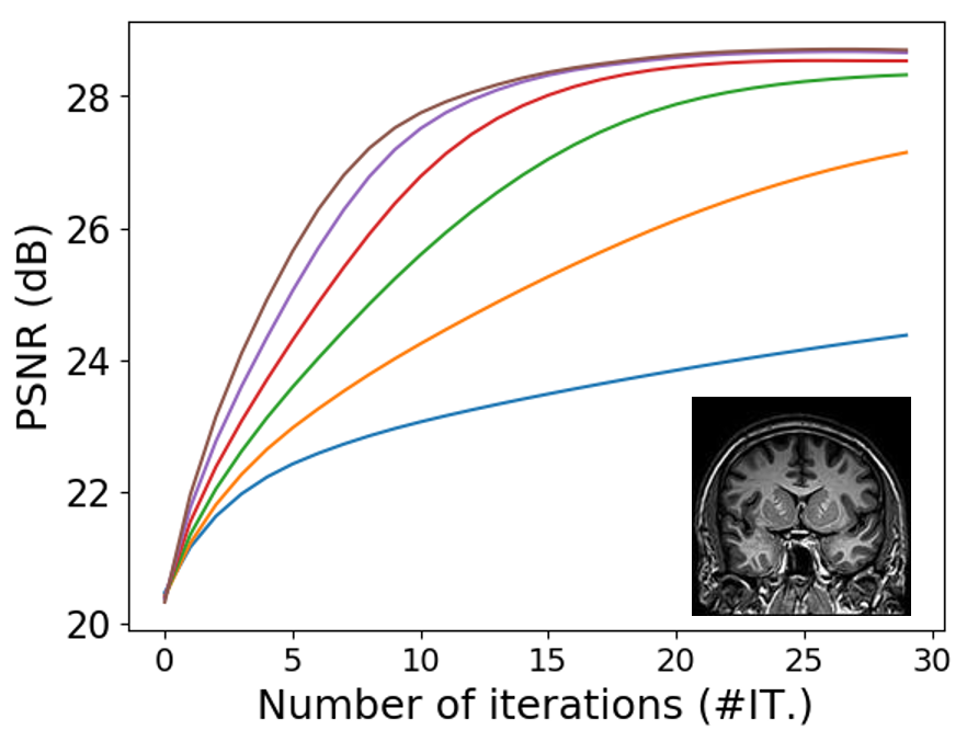
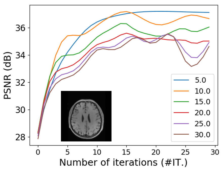
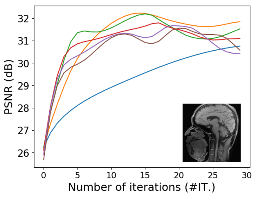
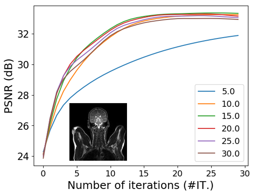
Sparse-View CT

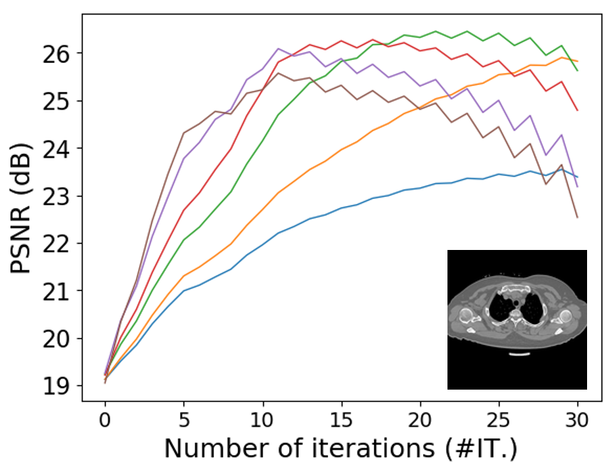
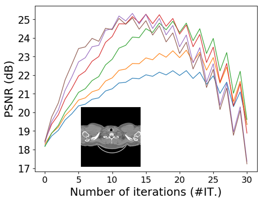
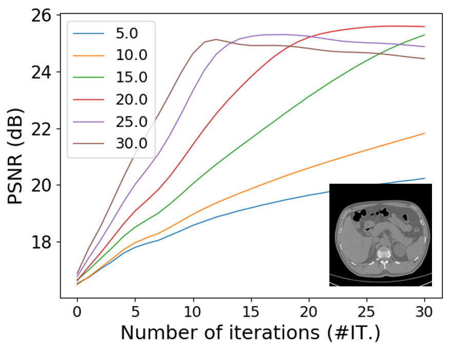
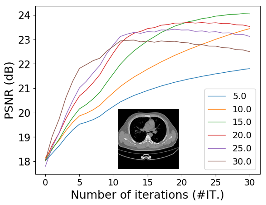
Figure 1: Performance comparison of PnP-ADMM using different denoising strengths. Plots display PSNR versus iterations on eight medical images on two applications (Compressed sensing MRI reconstruction with 20% sampling rate and sparse-view CT reconstruction using 30 views). From the PSNR curves, one can observe that each image prefers different denoising strengths and sometimes even requires early stopping to reach the optimal performance. (Best viewed with zoom)

Whilst a PnP framework offers promising image recovery results, it suffers a major drawback that its performance is highly sensitive to the internal parameter selection, which generically includes the denoising strength (of the denoiser) $\sigma$ and the termination time $\tau$, and others specified by the given optimization scheme (e.g., the penalty parameter $\mu$ in (8)). The body of literature often utilizes manual tweaking, e.g.,  (Rick Chang et al., 2017; Meinhardt et al., 2017) or handcrafted criteria, e.g.,  (Chan et al., 2017; Zhang et al., 2017b; Eksioglu, 2016; Tirer and Giryes, 2018) to select parameters for each specific problem setting. However, manual parameter tweaking requires several trials, which can be very cumbersome and time-consuming. Semi-automated handcrafted criteria (e.g., monotonically decreasing the denoising strength) can, to some degree, ease the burden of exhaustive searches of large parameter spaces, but often lead to sub-optimal local minima. Moreover, the optimal parameter setting differs from image to image, depending on the measurement model, the noise level, the noise type and the unknown image itself. These differences are illustrated in Figure 1, where peak signal-to-noise ratio (PSNR) curves are displayed for eight images on two applications (compressed sensing MRI and CT reconstruction) under varying denoising strengths.

1.3 Contributions

This work addresses the challenge of how to deal with the manual parameter tuning problem in a PnP framework. To this end, we formulate the internal parameter selection as a sequential decision-making problem, where a policy is adopted to select a sequence of internal parameters to guide the optimization. This formulation can be naturally fit into a reinforcement learning (RL) framework, where a policy agent seeks to map observations to actions, with the aim of maximizing cumulative reward. The reward reflects the to do or not to do events for the agent, and a desirable high reward can be obtained if the policy leads to faster convergence and better restoration accuracy.

We demonstrate, through rigorous numerical and visual experiments, the advantage of our algorithmic approach on compressed sensing MRI, sparse-view CT, single-photon imaging, and phase retrieval problems. We show that the policy allows to well approximate the intrinsic function that maps the input state to its optimal parameter setting. By using the learned policy, the guided optimization can reach comparable results to the ones using oracle parameters tuned via the inaccessible ground truth. An overview of our algorithm instantiated by PnP-ADMM is exhibited in Figure 2. Though the majority of results in this paper are given by PnP-ADMM, we also show our generic approach can be extended to a wide range of PnP-type algorithms, including but not limited to the plug-and-play proximal gradient method (PGM) (Sun et al., 2019b), half-quadratic splitting (HQS) (Zhang et al., 2017b), regularization by denoising (RED) (Romano et al., 2017) as well as denoising-based approximate message passing (D-AMP) (Metzler et al., 2016b). All the experiments collectively suggest the effectiveness of our algorithm in terms of both convergence speed and reconstruction accuracy.

The main contributions in this work are as follows:

1. We present a tuning-free plug-and-play (TFPnP) framework that can customize parameters towards a diverse range of imaging problems, and achieve faster practical convergence and better empirical performance than handcrafted criteria.

2. We introduce an efficient mixed model-free and model-based RL algorithm. It can optimize jointly the discrete termination time, and the continuous parameters e.g., denoising strength, penalty parameters, and step size, etc.

3. We validate our approach with an extensive range of numerical and visual experiments and show our generic method is applicable to a wide spectrum of PnP-type algorithms. We also show that our well-designed approach leads to better results than state-of-the-art techniques on compressed sensing MRI, sparse-view CT, single-photon imaging, and phase retrieval.

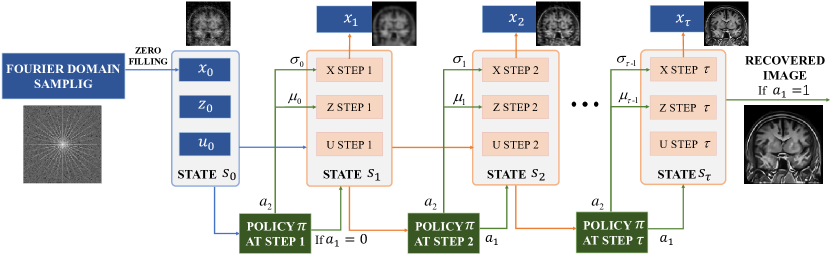
Figure 2: Workflow of our proposed tuning-free plug-and-play framework instantiated by the PnP-ADMM algorithm, in which we formulate the internal parameter selection as a sequential decision-making problem. The visualization displays the example case for fast MRI reconstruction.

The remainder of this paper is organized as follows. In Section 2, we provide an overview of PnP algorithmic techniques and other related philosophies. Section 3 introduces our TFPnP approach for automated parameter selection in a PnP framework. Main experimental results on four inverse imaging problems are presented in Section 4, followed by further investigation of our TFPnP algorithm and its extensions to several PnP-type methods in Section 5 and 6, respectively. Conclusion and future work are drawn in Section 7. A preliminary version of this work was presented as a conference paper in (Wei et al., 2020a).

2 Related Work

In this section, we first provide a brief overview of several important developments of PnP techniques. Then we review related works of other categories, which include automated parameter selection, algorithm unrolling as well as reinforcement learning for image recovery.

Plug-and-play (PnP) Techniques

The definitional concept of PnP was first introduced in (Danielyan et al., 2010; Zoran and Weiss, 2011; Venkatakrishnan et al., 2013). It has attracted great attention owing to its effectiveness and flexibility to handle a wide range of inverse imaging problems. Following this philosophy, the body of literature can be roughly categorized in terms of six aspects including proximal algorithms, denoiser priors, imaging applications, theoretical (convergence) analysis, and other two PnP-type frameworks (regularization by denoising (RED) (Romano et al., 2017) and denoising-based approximate message passing (D-AMP) (Metzler et al., 2016b)). Note that the PnP with learning-based denoisers also belongs to a broader class of methods coined as learning to optimize, whose overview is provided in (Chen et al., 2021).

• Proximal algorithms.  Initially, PnP was proposed to be combined with ADMM algorithm (Venkatakrishnan et al., 2013). Later on, extensions to other first-order proximal splitting algorithms are studied including half-quadratic splitting (Zhang et al., 2017b), primal-dual method (Ono, 2017), accelerated proximal gradient method (Kamilov et al., 2017) as well as their stochastic variants (Sun et al., 2019b, 2020).

• Denoising priors.  A key building block of PnP framework is the denoising algorithm. Over the years a wide range of denoisers have been used for the PnP framework, such as BM3D (Dar et al., 2016; Rond et al., 2016; Sreehari et al., 2016; Chan et al., 2017), sparse representation (Brifman et al., 2016), patch-based Wiener filtering (Venkatakrishnan et al., 2013), nonlocal means (Venkatakrishnan et al., 2013; Sreehari et al., 2016), Gaussian mixture models (Teodoro et al., 2016, 2018), weighted nuclear norm minimization (Kamilov et al., 2017), and deep learning-based denoisers (Meinhardt et al., 2017; Zhang et al., 2017b; Rick Chang et al., 2017; Zhang et al., 2020b).

• Imaging applications.  PnP methods reported empirical success on a large variety of imaging applications such as bright field electronic tomography (Sreehari et al., 2016), diffraction tomography (Sun et al., 2019b; Wu et al., 2020), nonlinear inverse scattering (Kamilov et al., 2017), low-dose CT imaging (He et al., 2018), compressed sensing MRI (Eksioglu, 2016), electron microscopy (Sreehari et al., 2017), single-photon imaging (Chan et al., 2017), phase retrieval (Metzler et al., 2018), Fourier ptychography microscopy (Sun et al., 2019c), light-field photography (Chun et al., 2019), hyperspectral sharpening (Teodoro et al., 2018), synthetic aperture radar image reconstruction (Alver et al., 2020), snapshot compressive imaging (Liu et al., 2018; Yuan et al., 2020), image/video processing—e.g., denoising, demosaicking, deblurring, super-resolution and inpainting (Heide et al., 2014; Rond et al., 2016; Meinhardt et al., 2017; Tirer and Giryes, 2018; Brifman et al., 2019; Zhang et al., 2019a, 2020b).

• Theoretical analysis.  The empirical success of PnP spurs researchers to study its theoretical properties (e.g., convergence), which is challenging as PnP priors are implicit and in general have no analytic mathematical expressions. Efforts along this direction were also made over recent years, to establish convergence via the symmetric gradient (Sreehari et al., 2016), the proper denoiser (Metzler et al., 2016b), the bounded denoiser (Chan et al., 2017) or the linear (possibly non-symmetric) denoiser (Gavaskar et al., 2021; Nair et al., 2021), and/or the nonexpansiveness assumptions (Sreehari et al., 2016; Teodoro et al., 2018; Sun et al., 2019b; Chan, 2019). Remarkably, the authors of (Ryu et al., 2019) show that PnP methods are contractive iterations under a mild Lipschitz condition on the denoisers. They further propose a technique namely real spectral normalization to enforce the proposed Lipschitz condition on training deep learning-based denoisers. Additionally, the works of (Buzzard et al., 2018; Chan, 2019) provide a consensus equilibrium view to PnP frameworks, shedding light on building connections among different PnP-type algorithms.

• Regularization by denoising.  Another framework closely related to PnP is so-called regularization by denoising (RED) (Romano et al., 2017), which uses the denoiser for defining the prior/regularizer explicitly. Under some conditions, the gradient of the regularizer has a very simple expression, which can be readily utilized in first-order optimization solvers, e.g., gradient descent and ADMM. For general cases where the conditions do not hold, the RED algorithms can be explained via a score-matching framework or consensus equilibrium (Reehorst and Schniter, 2018), or reformulated as a convex optimization problem via fixed-point projection (Cohen et al., 2020). A provably convergent block-coordinate RED is introduced in (Sun et al., 2019a) to tackle large-scale image recovery problems by a sequence of random partial updates. It is further extended into the asynchronous version (Sun et al., 2021) for parallel and distributed implementations.

• Denoising-based approximate message passing.  Different from the original PnP based on certain proximal splitting algorithms, denoising-based approximate message passing (D-AMP) (Metzler et al., 2016b), as another PnP-type framework, derives from the AMP algorithm that is built upon the loopy belief propagation in graphical models (Donoho et al., 2009, 2010a, 2010b; Rangan, 2010, 2011). The main appealing feature of the AMP algorithm is that for compressed sensing with i.i.d. sub-Gaussian measurement matrices, the method exhibits fast convergence with precise analytic characterizations on the algorithm behavior known as state evolution (Bayati and Montanari, 2011), which leads to near optimal tuning of internal parameters using Stein’s unbiased risk estimator (SURE) (Guo and Davies, 2015). The AMP, however, is fragile in that even small deviations from the i.i.d. sub-Gaussian model can cause the algorithm to diverge. Although many extensions have been proposed to work with a far broader class of matrices (Cakmak et al., 2014; Manoel et al., 2015; Ma and Ping, 2017; Rangan et al., 2019a; Millard et al., 2020; Metzler and Wetzstein, 2021), the algorithm’s behavior is still largely intractable under general measurement matrices (Rangan et al., 2016, 2019b), which seriously limits its application scope in practice.

Differing from these aspects, in this work we focus on the challenge of parameter selection in PnP, where a bad choice of parameters often leads to severe degradation of the results (Romano et al., 2017; Chan et al., 2017). Unlike existing semi-automated parameter tuning criteria (Wang and Chan, 2017; Chan et al., 2017; Zhang et al., 2017b; Eksioglu, 2016; Tirer and Giryes, 2018), our method is fully automatic and is purely learned from the data, which significantly eases the burden of manual parameter tuning.

Automated Parameter Selection

Choosing appropriate regularization parameters (or automated parameter selection in general) is a long-standing yet unresolved problem raised in a variety of domains such as signal/image processing, machine learning, and statistics communities. The existing methods for automatic parameter setting in literature can be broadly classified into four categories: 1) based on the discrepancy principle (Morozov, 1966; Karl, 2005), 2) the L-curve method (Hansen, 1992; Hansen and O’Leary, 1993; Vogel, 1996; Regińska, 1996; Hansen, 1999), 3) the generalized cross validation (GCV) (Golub et al., 1979; Wahba, 1990; Reeves, 1994; O’Sullivan and Wahba, 1985; Ramani et al., 2012), and 4) the Stein’s unbiased risk estimator (SURE) (Stein, 1981; Donoho and Johnstone, 1995; Blu and Luisier, 2007; Raphan and Simoncelli, 2008; Giryes et al., 2008; Vonesch et al., 2008; Eldar, 2008; Ramani et al., 2008; Giryes et al., 2011; Ramani et al., 2012; Mousavi et al., 2013; Bayati et al., 2013; Guo and Davies, 2015; Mousavi et al., 2018). The effectiveness of the former three approaches is often limited to linear reconstruction algorithms using e.g., Tikhonov regularization (Hansen and O’Leary, 1993; Golub et al., 1979). State-of-the-arts are therefore attributed to SURE-based methods, which provide an unbiased estimate of mean-square error (MSE) for parameter tuning, considering certain analytical regularizers, e.g., smoothed versions of the $\ell_{p}$ norm (Eldar, 2008; Giryes et al., 2011), or general convex functions (Ramani et al., 2012). Given more sophisticated non-convex and learned priors, the SURE is often restricted to AMP algorithms for compressed sensing applications due to the Gaussian noise assumption (Metzler et al., 2016b). Our method, instead, is generally applicable to almost every PnP-type algorithm for a wide range of inverse imaging problems.

Algorithm Unrolling

Perhaps the most confusable concept to PnP in the deep learning era is so-called algorithm unrolling methods (a.k.a. deep unfolding or unrolled optimization) (Gregor and LeCun, 2010; Hershey et al., 2014; Wang et al., 2016; Yang et al., 2016; Zhang and Ghanem, 2018; Diamond et al., 2017; Metzler et al., 2017a; Lefkimmiatis, 2018; Yang and Sun, 2018; Adler and Oktem, 2018; Mardani et al., 2018; Aggarwal et al., 2018; Dong et al., 2018; Xie et al., 2019; Gilton et al., 2019; Liu et al., 2019; Zhang et al., 2020a; Aggarwal and Jacob, 2020; Li et al., 2020; Lecouat et al., 2020; Dong et al., 2021; Huang et al., 2021; Liu et al., 2021), which explicitly unroll/truncate iterative optimization algorithms into learnable deep architectures. In this way, the denoiser prior and other internal parameters are treated as trainable parameters, meanwhile, the number of iterations has to be fixed to enable end-to-end training. By contrast, our TFPnP approach can adaptively select a stopping time and other internal parameters given varying input states. We refer interested readers to (Monga et al., 2021) for a thorough review of this topic.

Reinforcement Learning for Image Recovery

Although Reinforcement Learning (RL) has been applied in a range of domains, from game playing (Mnih et al., 2013; Silver et al., 2016) to robotic control (Schulman et al., 2015), only few works have successfully employed RL to the image recovery tasks. The study in (Yu et al., 2018) learned an RL policy to select appropriate tools from a toolbox to progressively restore corrupted images. The work of (Zhang et al., 2019b) proposed a recurrent image restorer whose endpoint was dynamically controlled by a learned policy. In (Furuta et al., 2019), authors used RL to select a sequence of classic filters to process images gradually. The work of (Yu et al., 2019) learned network path selection for image restoration in a multi-path CNN. In contrast to these works, we apply a mixed model-free and model-based deep RL approach to automatically select the parameters for the PnP image recovery algorithm.

3 Tuning-free Plug-and-Play Proximal Algorithm

In this section, we elaborate on our tuning-free PnP proximal algorithm described in  (7)-(9), which contains three main parts. Firstly, we describe how the automated parameter selection is driven. Secondly, we introduce our environment model. Finally, we introduce policy learning, which is guided by a mixed model-free and a model-based RL. We remark that, though our presentation on  (7)-(9) is for ADMM, our methodology can be adapted to other proximal algorithms, see Section 6 for more examples.

3.1 RL Formulation for Automated Parameter Selection

Our aim is to automatically select a sequence of parameters $(\sigma_{0},\mu_{0},\sigma_{1},\mu_{1},\cdots,\sigma_{\tau-1},\mu_{\tau-1}$) to guide the optimization (7)-(9) such that the recovered image $x^{\tau}$ is close to the underlying image $x$. We formulate this problem as a Markov decision process (MDP), which can be addressed via reinforcement learning (RL).

We denote the MDP by the tuple $(\mathcal{S},\mathcal{A},p,r)$, where $\mathcal{S}$ is the state space, $\mathcal{A}$ is the action space, $p$ is the transition function describing the environment dynamics, and $r$ is the reward function. Specifically, for our task, $\mathcal{S}$ is the space of optimization variable states, which includes the initialization $(x_{0},z_{0},u_{0})$ and all intermediate results $(x_{k},z_{k},u_{k})$ in the optimization process. $\mathcal{A}$ is the space of internal parameters, including both discrete termination time $\tau$ and the continuous denoising strength/penalty parameters ($\sigma_{k}$, $\mu_{k}$). The transition function $p:\mathcal{S}\times\mathcal{A}\to\mathcal{S}$ maps input state $s\in\mathcal{S}$ to its outcome state $s^{\prime}\in\mathcal{S}$ after taking action $a\in\mathcal{A}$. The state transition can be expressed as $s_{t+1}=p(s_{t},a_{t})$, which is composed of one or several iterations in the optimization. On each transition, the environment emits a reward in terms of the reward function $r:S\times\mathcal{A}\to\mathbb{R}$, which evaluates actions given the state. Applying a sequence of parameters to the initial state $s_{0}$ results in a trajectory $T$ of states, actions and rewards, i.e., $T=\{s_{0},a_{0},r_{0},\cdots,s_{N},a_{N},r_{N}\}$. Given a trajectory $T$, we define the return $R_{t}$ as the summation of discounted rewards after $s_{t}$, which reads:

$$R_{t}=\sum_{t^{\prime}=0}^{N-t}\rho^{t^{\prime}}r(s_{t+t^{\prime}},a_{t+t^{\prime}}),$$ (10)

where $\rho\in[0,1]$ is a discount factor and prioritizes earlier rewards over later ones.

Our goal is to learn a policy $\pi$, denoted as $\pi(a|s):\mathcal{S}\to\mathcal{A}$ for the decision-making agent, in order to maximize the objective defined as

$$J\left(\pi\right)=\mathbb{E}_{s_{0}\sim S_{0},T\sim\pi}\left[R_{0}\right],$$ (11)

where $\mathbb{E}$ represents expectation, $s_{0}$ is the initial state, and $S_{0}$ is the corresponding initial state distribution. Intuitively, the objective describes the expected return over all possible trajectories induced by the policy $\pi$. The expected return on states and state-action pairs under the policy $\pi$ are defined by state-value functions $V^{\pi}$ and action-value functions $Q^{\pi}$ respectively, i.e.,

$$V^{\pi}\left(s\right) =\mathbb{E}_{T\sim\pi}\left[R_{0}|s_{0}=s\right],$$ (12)

$$Q^{\pi}\left(s,a\right) =\mathbb{E}_{T\sim\pi}\left[R_{0}|s_{0}=s,a_{0}=a\right].$$ (13)

In our task, we decompose actions into two parts, i.e., $a=(a_{1},a_{2})$, which includes a discrete decision $a_{1}$ on termination time $\tau$ and a continuous decision $a_{2}$ on denoising strength $\sigma$ and penalty parameter $\mu$. The policy also consists of two sub-policies: $\pi=(\pi_{1},\pi_{2})$, a stochastic policy and a deterministic policy that generate $a_{1}$ and $a_{2}$ respectively. The role of $\pi_{1}$ is to decide whether to terminate the iterative algorithm when the next state is reached. It samples a boolean-valued outcome $a_{1}$ from a two-class categorical distribution $\pi_{1}(\cdot|s)$, whose probability mass function is calculated from the current state $s$. We move forward to the next iteration if $a_{1}=0$, otherwise, the optimization would be terminated to output the final state. Compared to the stochastic policy $\pi_{1}$, we treat $\pi_{2}$ deterministically, i.e., $a_{2}=\pi_{2}(s)$. Since $\pi_{2}$ is differentiable with respect to the environment, its gradient can be precisely estimated.

3.2 Environment Model

In RL the environment is characterized by two components, i.e., the environment dynamics and reward function. In our task, the environment dynamics is described by the transition function $p$ related to the PnP-ADMM. Here, we detail the setting of the PnP-ADMM as well as the reward function used for training policy.

Denoiser Prior

A differentiable environment makes policy learning more efficient. To make the environment differentiable with respect to $\pi_{2}$, we take a convolutional neural network (CNN) denoiser as the image prior. In practice, we use a residual U-Net (Ronneberger et al., 2015) architecture, which was originally designed for medical image segmentation and was recently found to be useful in image denoising (Brooks et al., 2019). Besides, we incorporate an additional tunable noise level map into the input as (Zhang et al., 2018), enabling us to provide continuous noise level control (i.e., different denoising strength) within a single network.

Proximal Operator of Data-fidelity Term

Enforcing consistency with measured data requires evaluating the proximal operator of $\mathcal{D}$ in (8). For inverse problems, there might exist fast solutions due to the special structure of the observation model. We adopt the fast solution if it is available (e.g., closed-form solution using fast Fourier transform, rather than the general matrix inversion), otherwise a single step of gradient descent is performed.

Transition Function

To reduce the computation cost, we define the transition function $p$ to involve $m$ iterations of the optimization. At each time step, the agent needs to decide the internal parameters for $m$ iterates. Larger $m$ would lead to coarser control of the termination time, but make the decision-making process more efficient. Its value is set to 5 empirically. To avoid the optimization loops infinitely, the maximum time step $N$ is set to 6 in our algorithm, leading to 30 iterations of the optimization at most.

Reward Function

To take both image recovery performance and runtime efficiency into account, we define the reward function as:

$$r(s_{t},a_{t})=\left[\zeta(p(s_{t},a_{t}))-\zeta(s_{t})\right]-\eta,$$ (14)

The first term, $\zeta(p(s_{t},a_{t}))-\zeta(s_{t})$, denotes the PSNR increment made by the policy, where $\zeta(s_{t})$ denotes the PSNR of the recovered image at step $t$. A higher reward is acquired if the policy leads to higher performance gain in terms of PSNR. The second term, $\eta$, implies penalizing the policy as it does not select to terminate at step $t$, where $\eta$ sets the degree of penalty. A negative reward is given if the PSNR gain does not exceed the degree of penalty, thereby encouraging the policy to early stop the iteration with diminishing returns. We set $\eta=0.05$ in our algorithm.

Layer name	Feature extractor	Output size
conv1	$3\times 3,64$	$64\times 64$
layer1	$\left[\begin{subarray}{c}3\times 3,\,64\\ 3\times 3,\,64\end{subarray}\right]\times 2$	$32\times 32$
layer2	$\left[\begin{subarray}{c}3\times 3,\,128\\ 3\times 3,\,128\end{subarray}\right]\times 2$	$16\times 16$
layer3	$\left[\begin{subarray}{c}3\times 3,\,256\\ 3\times 3,\,256\end{subarray}\right]\times 2$	$8\times 8$
layer4	$\left[\begin{subarray}{c}3\times 3,\,512\\ 3\times 3,\,512\end{subarray}\right]\times 2$	$4\times 4$
avgpool	$4\times 4$ average pooling	$1\times 1$

Table 1: Network configuration of the feature extractor of our policy and value networks. We refer to ‘$3\times 3,\,64$’ as $3\times 3$ kernel size and 64 output feature maps. Each layer is composed of two building blocks of the residual network. The building block consists of two convolutional layers with batch normalization (BN) (Ioffe and Szegedy, 2015), ReLU activation, and skip connection. The BN and ReLU are replaced by weight normalization (Salimans and Kingma, 2016) and TReLU (Xiang and Li, 2017) respectively in the value network.

3.3 RL-based Policy Learning

In this section, we present a mixed model-free and model-based RL algorithm to learn the policy. Specifically, model-free RL (agnostic to the environment dynamics) is used to train $\pi_{1}$, while model-based RL is utilized to optimize $\pi_{2}$ to make full use of the environment model. We employ the actor-critic framework (Sutton et al., 2000), which uses a policy network $\pi_{\theta}(a_{t}|s_{t})$ (actor) and a value network $V_{\phi}^{\pi}(s_{t})$ (critic) to formulate the policy and the state-value function respectively.

The design principle of a policy/value network is to make it simple yet effective. For convenience, we follow (Huang et al., 2019) that uses residual structures similar to ResNet-18 (He et al., 2016) as the feature extractor in the policy and value networks, followed by fully-connected layers and activation functions to produce desired outputs. The network configuration of the feature extractor of the policy and value networks is listed in Table 1. To make the policy aware of the problem settings (Silver et al., 2016), we encode the auxiliary setting-related information (i.e., the measurement noise level and the number of steps that have been taken so far in the optimization process) into the input of the policy network. Notice the input of our policy network is the optimization variables ($x_{k},z_{k},u_{k}$) with spatial size $H\times W$. To encode the extra scalar-type information into the policy network, we augment the input with the same spatial-sized feature maps with all entries equal to the same value representing the auxiliary information. These values are normalized into [0, 1] range to avoid inconsistent magnitude. It is worth noting that the extra computation cost of the policy network is marginal, compared with the iteration cost in the PnP-ADMM (7)-(9).

The policy and the value networks are learned in an interleaved manner. For each gradient step, we optimize the value network parameters $\phi$ by minimizing

$$L_{\phi}=\mathbb{E}_{s\sim B,a\sim\pi_{\theta}(s)}\left[\frac{1}{2}(r(s,a)+\gamma V^{\pi}_{\hat{\phi}}(p(s,a))-V^{\pi}_{\phi}(s))^{2}\right],$$ (15)

where $B$ is the distribution of previously sampled states, practically implemented by a state buffer. This partly serves as a role of the experience replay mechanism (Lin, 1992), which is observed to “smooth” the training data distribution (Mnih et al., 2013). The update makes use of a target value network $V^{\pi}_{\hat{\phi}}$, where $\hat{\phi}$ is the exponentially moving average of the value network weights and has been shown to stabilize training (Mnih et al., 2015).

The policy network has two sub-policies, which employs shared convolutional layers to extract image features, followed by two separated groups of fully-connected layers to produce termination probability $\pi_{1}(\cdot|s)$ (after softmax) or denoising strength/penalty parameters $\pi_{2}(s)$ (after sigmoid). We denote the parameters of the sub-policies as $\theta_{1}$ and $\theta_{2}$ respectively, and we seek to optimize $\theta=(\theta_{1},\theta_{2})$ so that the objective $J(\pi_{\theta})$ is maximized. The policy network is trained using policy gradient methods (Peters and Schaal, 2006). The gradient of $\theta_{1}$ is estimated by a likelihood estimator in a model-free manner, while the gradient of $\theta_{2}$ is estimated relying on backpropagation via environment dynamics in a model-based manner. Specifically, for discrete termination time decision $\pi_{1}$, we apply the policy gradient theorem (Sutton et al., 2000) to obtain unbiased Monte Carlo estimate of $\triangledown_{\theta_{1}}J(\pi_{\theta})$ using the advantage function $A^{\pi}(s,a)=Q^{\pi}(s,a)-V^{\pi}(s)$ as target, which is computed as:

$$\triangledown_{\theta_{1}}J(\pi_{\theta})= \mathbb{E}_{s\sim B,a\sim\pi_{\theta}(s)}\left[\triangledown_{\theta_{1}}\mathrm{log}\,\pi_{1}(a_{1}|s)\,A^{\pi}(s,a)\right].$$ (16)

For continuous denoising strength and penalty parameter selection $\pi_{2}$, we utilize the deterministic policy gradient theorem (Silver et al., 2014) to formulate its gradient which reads:

$$\triangledown_{\theta_{2}}J(\pi_{\theta})= \mathbb{E}_{s\sim B,a\sim\pi_{\theta}(s)}\left[\triangledown_{a_{2}}\,Q^{\pi}(s,a)\triangledown_{\theta_{2}}\pi_{2}(s)\right],$$ (17)

where we approximate the action-value function $Q^{\pi}(s,a)$ by $r(s,a)+\gamma V_{\phi}^{\pi}(p(s,a))$ given its unfolded definition (Sutton and Barto, 2018).

Using the chain rule, we can directly obtain the gradient of $\theta_{2}$ by backpropagation via the reward function, the value network and the transition function, in contrast to relying on the gradient backpropagated from only the learned action-value function in the model-free DDPG algorithm (Lillicrap et al., 2016).

The detailed training algorithm for our policy learning is summarized in Algorithm 1. It requires an image dataset $D$, a degradation operator $g(\cdot)$, learning rates $l_{\theta}$, $l_{\phi}$, and a weight parameter $\beta$. To sample initial states $s_{0}$, we define the degradation operator $g(\cdot)$ as a composition of a forward model and an initialization function. The forward model maps the underlying image $x$ to its observation $y$, while the initialization function generates the initial estimate $x_{0}$ from the observation $y$. For linear inverse problems, $g(\cdot)$ is typically defined by the composition of the forward operator and the adjoint operator of the problem (for example, $g(\cdot)$ is a composition of the partially-sampled Fourier transform and the inverse Fourier transform in CS-MRI). For nonlinear inverse problem—phase retrieval, we employ the HIO algorithm (Fienup, 1982) as the initialization function.

Algorithm 1 Training Scheme

0:  Image dataset $D$, degradation operator $g(\cdot)$, learning rates $l_{\theta}$, $l_{\phi}$, weight parameter $\beta$.

1:  Initialize network parameters $\theta$, $\phi$, $\hat{\phi}$ and state buffer $B$.

2:  for each training iteration do

3:     sample initial state $s_{0}$ from $D$ via $g(\cdot)$

4:     for environment step $t\in[0,N)$ do

5:        $a_{t}\sim\pi_{\theta}(a_{t}|s_{t})$

6:        $s_{t+1}\sim p(s_{t+1}|s_{t},a_{t})$

7:        $B\leftarrow B\cup\{s_{t+1}\}$

8:        break if the boolean outcome of $a_{t}$ equals to 1

9:     end for

10:     for each gradient step do

11:        sample states from the state buffer $B$

12:        $\theta_{1}\leftarrow\theta_{1}+l_{\theta}\triangledown_{\theta_{1}}J(\pi_{\theta})$

13:        $\theta_{2}\leftarrow\theta_{2}+l_{\theta}\triangledown_{\theta_{2}}J(\pi_{\theta})$

14:        $\phi\leftarrow\phi-l_{\phi}\triangledown_{\phi}L_{\phi}$

15:        $\hat{\phi}\leftarrow\beta\phi+(1-\beta)\hat{\phi}$

16:     end for

17:  end for

17:  Learned policy network $\pi_{\theta}$

4 Experimental Results

In this section, we first detail the implementation of our TFPnP algorithm, then present experimental results on three inverse imaging applications. Both linear (i.e., Compressed Sensing MRI and Sparse-view CT) and nonlinear (i.e., Phase Retrieval) inverse imaging problems are explored to demonstrate the robustness and applicability of our algorithm.

4.1 Implementation Details

Our TFPnP algorithm requires two training stages sequentially, i.e., the denoiser (denoising network) training stage and the policy learning stage. To train the denoising network, we follow the common practice that uses 87,000 overlapping patches (with size $128\times 128$) drawn from 400 images from the BSD dataset (Martin et al., 2001). For each patch, we add white Gaussian noise with noise level sampled from $[1,50]$. The denoising networks are trained with 50 epochs using $L_{1}$ loss and Adam optimizer (Kingma and Ba, 2014) with batch size 32. The base learning rate is set to $10^{-4}$ and halved at epoch 30, then reduced to $10^{-5}$ at epoch 40.

To train the policy network (and an auxiliary value network only used during training), we use the 17,125 resized images with size $128\times 128$ from the PASCAL VOC dataset (Everingham et al., 2014). We use Adam optimizer with batch size 48 and 2500 training iterations. We start by setting the learning rates $l_{\theta}$, $l_{\phi}$ for updating the policy network $\pi_{\theta}$ and the value network $V_{\phi}^{\pi}$ to $1\times 10^{-4}$ and $5\times 10^{-5}$ respectively. Then we reduced these values to $5\times 10^{-5}$ and $1\times 10^{-5}$ respectively at training iteration 1600. The value network learning makes use of a target value network, which is a soft copy of the value network itself. The weight parameter $\beta$ for softly updating the target value network is set to $10^{-3}$ (see line 15 in Algorithm 1). In each training iteration, we alternate between collecting states (in a state buffer) from the environment with the current policy and updating the network parameters using policy gradients from batches sampled from the state buffer $B$. Ten gradient steps are performed at each training iteration.

For each inverse imaging application, only a single policy network is trained to tackle different imaging settings, for instance, one policy network is learned to handle multiple sampling ratios (with 2$\times$/4$\times$/8$\times$ acceleration) and noise levels (5/10/15) simultaneously for the CS-MRI application.

Method	DnCNN	MemNet	U-net
Denoising Performance	27.18	27.32	27.40
PnP Performance	25.43	25.67	25.76
Run Times (ms)	8.09	64.65	5.65

Table 2: Numerical comparison of different CNN-based denoisers. We show the results of Gaussian denoising performance (PSNR) under noise level $\sigma=50$, the CS-MRI performance (PSNR) when plugged into the PnP-ADMM, and the GPU runtime (millisecond) of denoisers when processing an image with size $256\times 256$.

	$2\times$		$4\times$		$8\times$
Policies	PSNR	#IT.	PSNR	#IT.	PSNR	#IT.
handcrafted	30.05	30.0	27.90	30.0	25.76	30.0
handcrafted∗	30.06	29.1	28.20	18.4	26.06	19.4
fixed	23.94	30.0	24.26	30.0	22.78	30.0
fixed∗	28.45	1.6	26.67	3.4	24.19	7.3
fixed optimal	30.02	30.0	28.27	30.0	26.08	30.0
fixed optimal∗	30.03	6.7	28.34	12.6	26.16	16.7
greedy	29.51	30.0	28.39	30.0	26.20	30.0
greedy∗	30.07	8.0	28.47	17.6	26.33	19.0
oracle	30.25	30.0	28.60	30.0	26.41	30.0
oracle∗	30.26	8.6	28.61	13.9	26.45	21.6
model-free	28.79	30.0	27.95	30.0	26.15	30.0
Ours	30.33	5.0	28.58	10.0	26.52	15.0

Table 3: Comparisons of different policies used in PnP-ADMM algorithm for CS-MRI on seven widely used medical images under various acceleration factors (2$\times$/4$\times$/8$\times$) and noise level 15. We show both PSNR and the number of iterations (#IT.) used to induce the results. * denotes to report the best PSNR over all iterations (i.e., with optimal early stopping). The best results are indicated by orange color and the second best results are denoted by blue color.

Dataset	$f$	$\sigma_{n}$	Traditional		Algorithm Unrolling		PnP
			RecPF	FCSA	ADMMNet	ISTANet	BM3D-MRI	IRCNN	Ours
Medical7	$2\times$	$5$	$32.46$	$31.70$	$33.10$	$34.58$	$33.33$	$34.67$	$35.10$
		$10$	$29.48$	$28.33$	$31.37$	$31.81$	$29.44$	$31.80$	$32.04$
		$15$	$27.08$	$25.52$	$29.16$	$29.99$	$26.90$	$29.96$	$30.33$
	$4\times$	$5$	$28.67$	$28.21$	$30.24$	$31.34$	$30.33$	$31.36$	$31.81$
		$10$	$26.98$	$26.67$	$29.20$	$29.71$	$28.30$	$29.52$	$29.86$
		$15$	$25.58$	$24.93$	$27.87$	$28.38$	$26.66$	$27.94$	$28.58$
	$8\times$	$5$	$24.72$	$24.62$	$26.57$	$27.65$	$26.53$	$27.32$	$28.31$
		$10$	$23.94$	$24.04$	$26.21$	$26.90$	$25.81$	$26.44$	$27.28$
		$15$	$23.18$	$23.36$	$25.49$	$26.23$	$25.09$	$25.53$	$26.52$
MICCAI	$2\times$	$5$	$36.39$	$34.90$	$36.74$	$38.17$	$36.00$	$38.42$	$38.61$
		$10$	$31.95$	$30.12$	$34.20$	$34.81$	$31.39$	$34.93$	$35.06$
		$15$	$28.91$	$26.68$	$31.42$	$32.65$	$28.46$	$32.81$	$33.12$
	$4\times$	$5$	$33.05$	$32.30$	$34.15$	$35.46$	$34.79$	$35.80$	$36.17$
		$10$	$30.21$	$29.56$	$32.58$	$33.13$	$31.63$	$32.99$	$33.38$
		$15$	$28.13$	$26.93$	$30.55$	$31.48$	$29.35$	$30.98$	$31.75$
	$8\times$	$5$	$28.35$	$28.71$	$30.36$	$31.62$	$31.34$	$31.66$	$32.69$
		$10$	$26.86$	$27.68$	$29.78$	$30.54$	$29.86$	$30.16$	$30.93$
		$15$	$25.70$	$26.35$	$28.83$	$29.50$	$28.53$	$28.72$	$29.75$

Table 4: Quantitative results (PSNR) of different CS-MRI methods under various acceleration factors $f$ and noise levels $\sigma_{n}$ on two datasets. The best results are indicated in orange color and the second best results are denoted in blue color.

RecPF	FCSA	ADMMNet	ISTANet	BM3D-MRI	IRCNN	Ours	Ground Truth
22.57	22.27	24.15	24.61	23.64	24.16	25.28	PSNR
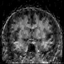
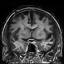
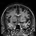
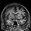
18.74	19.23	20.48	21.37	20.62	20.91	22.02	PSNR
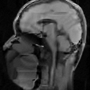
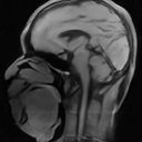
24.89	24.47	26.85	27.90	26.72	27.74	28.65	PSNR

Figure 3: Visual and numerical CS-MRI reconstruction comparison against the state-of-the-art techniques on medical images. The numerical values denote the PSNR obtained by each technique. (Details are better appreciated on screen).

4.2 Compressed Sensing MRI

Magnetic resonance imaging (MRI) (Wright, 1997) is an essential imaging modality for diagnosing and evaluating a host of conditions and diseases, but suffers from slow data acquisition. Compressed sensing MRI (CS-MRI) (Lustig et al., 2008) accelerates MRI by acquiring less data through subsampling. Recovering high-quality images from undersampled MRI data is an ill-posed inverse imaging problem. The forward model of CS-MRI can be mathematically described as: $y=\mathcal{F}_{p}x+\omega$, where $x\in\mathbb{C}^{N}$ is the underlying image, the operator $\mathcal{F}_{p}:\mathbb{C}^{N}\rightarrow\mathbb{C}^{M}$, with $M<N$, denotes the partially-sampled Fourier transform, and $\omega\sim\mathcal{N}\left(0,\sigma_{n}I_{M}\right)$ is the additive white Gaussian noise. The data-fidelity term, for the MRI reconstruction, is $\mathcal{D}(x)=\frac{1}{2}\|y-\mathcal{F}_{p}x\|^{2}$ whose proximal operator is described in (Eksioglu, 2016).

Denoiser Priors

To show how denoiser priors affect the performance of the PnP, we train three state-of-the-art CNN-based denoisers, i.e., DnCNN (Zhang et al., 2017a), MemNet (Tai et al., 2017) and residual U-net (Ronneberger et al., 2015), with a tunable noise level map. We compare both the Gaussian denoising performance and the PnP performance using these denoisers. As shown in Table 2, the residual U-net and MemNet consistently outperform DnCNN in terms of denoising and CS-MRI. It seems to imply a better Gaussian denoiser is also a better denoiser prior for the PnP framework. Since U-net is significantly faster than MemNet and yields slightly better performance, we choose U-net as our denoiser prior.

Comparisons of Different Policies

We start by providing some insights of our learned policy by comparing the performance of PnP-ADMM with different policies: i) the handcrafted policy used in IRCNN (Zhang et al., 2017b); ii) the fixed policy that uses fixed parameters ($\sigma=15$, $\mu=0.1$); iii) the fixed optimal policy that adopts fixed parameters searched to maximize the average PSNR across all testing images; iv) the greedy policy that selects parameters in a greedy manner to maximize the PSNR at each iteration during optimization; v) the oracle policy that uses different parameters for different images such that the PSNR of each image is maximized and vi) our learned policy network to optimize parameters for each image. We remark that all compared policies are run for 30 iterations whilst ours automatically chooses the termination time.

To understand the usefulness of the early stopping mechanism, we also report the results of these policies with optimal early stopping. Moreover, we analyze whether the model-based RL benefits our algorithm by comparing it with the learned policy by model-free RL whose $\pi_{2}$ is optimized using the model-free DDPG algorithm (Lillicrap et al., 2016).

The results of all aforementioned policies are provided in Table 3. We can see that bad choice of parameters (see “fixed”) induces poor results, in which the early stopping is required to rescue performance (see “fixed^∗”). When the parameters are properly assigned, the early stopping would be helpful to reduce computation cost. The greedy policy serves as an upper bound of SURE-based parameter tuning methods if applicable, which however often yields suboptimal results. Our learned policy leads to fast practical convergence as well as excellent performance, sometimes even outperforms the oracle policy tuned via inaccessible ground truth (in $2\times$ and $8\times$ case). We note this is owing to the varying parameters across iterations generated automatically in our algorithm, which yield extra flexibility than constant parameters over iterations. Besides, we find that the learned model-free policy produces suboptimal denoising strength/penalty parameters compared with our mixed model-free and model-based policy, and it also fails to learn early stopping.

Comparisons with State-of-the-arts

We compare our method against six state-of-the-art methods for CS-MRI, including the traditional optimization-based approaches (RecPF (Yang et al., 2010) and FCSA (Huang et al., 2010)), the PnP approaches (BM3D-MRI (Eksioglu, 2016) and IRCNN (Zhang et al., 2017b)), and the unrolling approaches (ADMMNet (Yang et al., 2016) and ISTANet (Zhang and Ghanem, 2018)). To keep comparison fair, for each algorithm unrolling method, only a single network is trained to tackle all the cases using the same dataset as ours. All parameters involved in the competing methods are manually tuned optimally or automatically chosen as described in the reference papers. Table 4 shows the method performance on two medical image datasets: 7 widely used medical images (Medical7) (Huang et al., 2010) and 50 medical images from MICCAI 2013 grand challenge dataset. The visual comparison can be found in Figure 3. It can be seen that our approach significantly outperforms the state-of-the-art PnP method (IRCNN) by a large margin, especially under the difficult $8\times$ case. In the low acceleration cases (e.g., $2\times$), our algorithm only runs 5 iterations to arrive at the desired performance, in contrast with 30 or 70 iterations required in IRCNN and BM3D-MRI respectively.

FBP	TV	FBPconv	RED-CNN	LPD	RPGD	Ours	Ground Truth
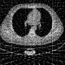
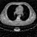
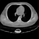
18.30	20.91	22.16	22.34	22.72	23.19	23.21	PSNR
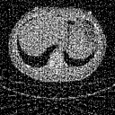
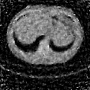
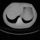
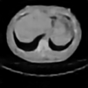
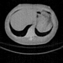
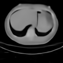
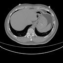
15.54	18.16	22.55	22.87	22.95	23.62	24.43	PSNR
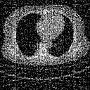
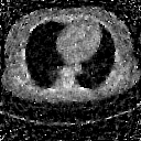
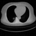
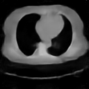
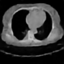
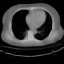
14.33	17.12	22.71	22.18	22.50	23.13	23.48	PSNR

Figure 4: Sparse-view CT reconstruction results and their corresponding PSNR values for all compared methods. The results are produced on several medical images using 30 views. (Best view on screen with zoom)

4.3 Sparse-View Computed Tomography

Computed tomography (CT) (Herman, 2009) utilizes X-ray measurements taken from different angles to produce tomographic images of a body, which is also widely used in clinical applications as MRI. Given the potential risk of X-ray radiation to the patient, low-dose CT has been intensively studied in response to concerns of patient safety in full-dose CT scans. Typically, low-dose CT scan can be achieved either by reducing the number of projection views (sparse-view CT) or by lowering the operating current of an X-ray tube. Here, we focus on the sparse-view CT reconstruction with the goal to reduce the number of views (or dose) for CT imaging while retaining the quality of full-dose reconstruction. The forward operator is given by the Radon transform (Natterer, 2001) that integrates the signal over a set of lines given by a sparse acquisition geometry. We implement Radon transform by the TorchRadon library (Ronchetti, 2020), which can be seamlessly integrated into PyTorch with full differentiability. We validate our method on a challenging case of sparse-view CT reconstruction, using a sparse 30-view parallel beam geometry with 182 detector pixels to generate projections, blended with varying amounts (5%/7.5%/10%) of Gaussian noise.

The competing methods for CT reconstruction include filtered backprojection (FBP) (Herman, 2009), total variation (TV) reconstruction (Sidky and Pan, 2008), RED-CNN (Chen et al., 2017), FBPconv (Jin et al., 2017), learned primal dual (LPD) reconstruction (Adler and Oktem, 2018) and RPGD (Gupta et al., 2018). The former two are the traditional methods, while the latter four are the state-of-the-art deep learning methods. For TV reconstruction, we adopt the PDHG solver (Chambolle and Pock, 2011) with optimally tuned parameters. For the learning-based methods, we train their models using the same dataset as ours, and manually tune configurations to achieve performance as higher as possible. The numerical and visual results are evaluated on 50 randomly selected lung CT images from the COVID-19 CT lung and infection segmentation dataset (Ma et al., 2020), shown in Table 5 and Figure 4 respectively. Our TFPnP algorithm yields considerably better results than state-of-the-arts (e.g., it outperforms the second-best method RPGD 0.4dB in terms of PSNR under 7.5% Gaussian noise setting), suggesting the effectiveness of our algorithm.

	$5\%$	$7.5\%$	$10\%$
Algorithms	PSNR	PSNR	PSNR
FBP	18.37	16.16	14.32
TV	21.47	19.17	16.95
FBPconv	23.00	22.94	22.86
RED-CNN	23.45	23.11	22.71
LPD	23.86	23.44	23.00
RPGD	24.29	23.82	23.38
Ours	24.50	24.23	23.72

Table 5: Quantitative results (PSNR) of Sparse-view (30 views) CT reconstruction with varying degrees (5%, 7.5%, 10%) of Gaussian noise added into the projections.

	$K=4$	$K=6$	$K=8$
Algorithms	PSNR	PSNR	PSNR
MLE	13.48	17.51	20.12
Chan et al.	25.11	27.26	28.67
Ryu et al.	25.26	27.80	29.18
Ours	25.55	28.47	30.32

Table 6: Quantitative results (PSNR) of single-photon imaging with different oversampling ratios ($K=4,6,8$)

4.4 Single-photon Imaging

Quanta imaging sensor (QIS) is an emerging class of solid-state imaging sensors that are capable of detecting individual photons in space and time (Fossum, 2011; Fossum et al., 2016). The principle of QIS is analogous to photographic film: photon flux hitting a pixel area of the single-photon detector, triggers a binary response (1-bit signal) revealing the intensity of light during exposure. The 1-bit measurements acquired by the QIS follow a quantized Poisson process, which must be “decoded” to recover the underlying image (Yang et al., 2011; Chan and Lu, 2014). QIS is a spatial oversampling device composed of many tiny single-photon detectors called jots. In each unit space, $K$ jots are used to acquire light corresponding to a pixel in the usual sense (e.g., a pixel in a CMOS sensor). By assuming homogeneous distribution of the light within each pixel, we consider single-photon imaging using a simplified QIS imaging model which relates the underlying image $x\in\mathbb{R}^{N}$ and the 1-bit measurements $y\in\mathbb{R}^{NK}$ as

$$y=\textbf{1}\left(z\geq 1\right),\quad z\sim\mathcal{P}\left(\alpha_{s}Gx\right)$$

where $G:\mathbb{R}^{N}\to\mathbb{R}^{NK}$ is an oversampling operator that duplicates each pixel to $K$ pixels, $\alpha_{s}\in\mathbb{R}$ is sensor gain, $\mathcal{P}$ denotes the Poisson distribution, $\textbf{1}(\cdot\geq 1)$ is an indicator function that executes binary quantization on threshold 1.

The goal is to reconstruct the unknown image of interest $x$ from the observed binary photons $y$. Given the log likelihood function of the quantized Poisson process (Yang et al., 2011), the corresponding data-fidelity term $\mathcal{D}$ can be defined as

$$\mathcal{D}(x)=\sum_{j=1}^{N}-K_{j}^{0}\mathop{\mathrm{log}}(e^{-\frac{\alpha_{s}x_{j}}{K}})-K_{j}^{1}\mathop{\mathrm{log}}(1-e^{-\frac{\alpha_{s}x_{j}}{K}}),$$ (18)

where $K_{j}^{1}=\sum_{i=1}^{K}y_{(j-1)K+i}$ and $K_{j}^{0}=\sum_{i=1}^{K}(1-y_{(j-1)K+i})$ denote the numbers of ones and zeros in the $j$-th unit pixel (containing $K$ jots) respectively. The proximal operator of (18) is given in (Chan and Lu, 2014), which requires a numerical scheme to address a root finding problem of a transcendental equation. In practice, we follow (Ryu et al., 2019) to use a vectorized bisection algorithm for root finding, and transplant their method into Pytorch with differentiable programming. The iteration times of bisection are empirically set to 10, as a good balance between computation precision and cost.

We consider three sets of experiments with different oversampling ratios ($K=4,6,8$ along both horizontal and vertical directions). The sensor gain is set as $\alpha_{s}=K^{2}$. For comparison, we choose the three existing algorithms, including the maximum likelihood estimation (MLE) method (Yang et al., 2011), and two PnP methods in (Chan et al., 2017) and (Ryu et al., 2019). The visual and numerical results are shown in Figure 5 and Table 6 respectively. From these results, one can observe that our method reconstructed the highest-quality images that closely resemble the ground truth, conforming with the quantitative assessment via PSNR.

Binary input	MLE	Chan et al.	Ryu et al.	Ours	Ground Truth
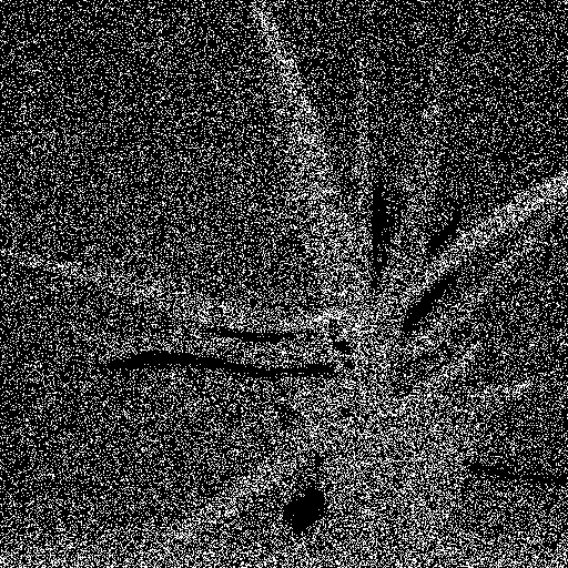
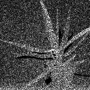
-	16.34	29.09	29.40	30.32	PSNR
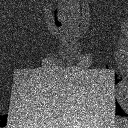
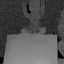
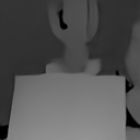
-	19.20	35.42	29.42	35.81	PSNR
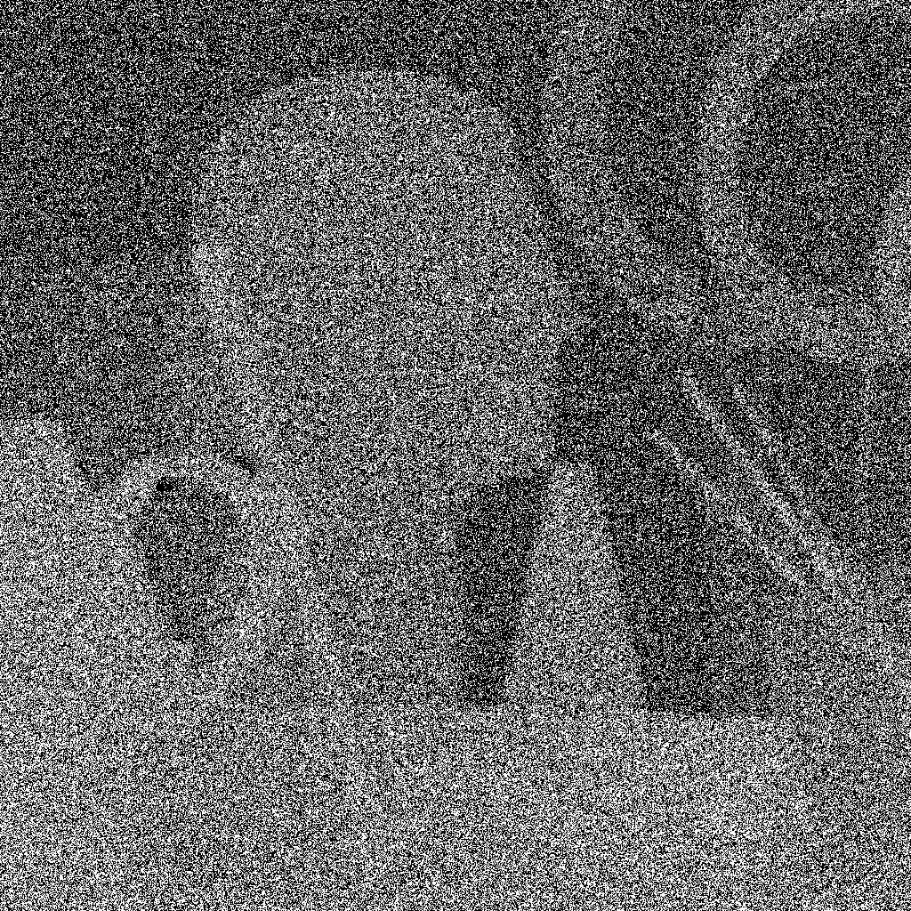
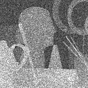
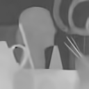
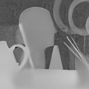
-	19.44	31.08	32.48	33.32	PSNR

Figure 5: Single-photon imaging results and their associated PSNR values for our technique and the compared methods. (Best view on screen with zoom)

HIO	WF	DOLPHIn	SPAR	BM3D-prGAMP	prDeep	Ours	Ground Truth
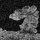
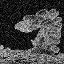
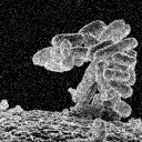
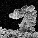
14.36	15.37	21.13	23.86	23.40	24.47	25.02	PSNR
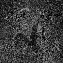
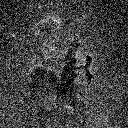
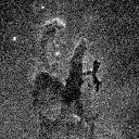
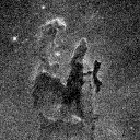
14.40	15.52	19.35	22.48	25.66	27.72	28.01	PSNR
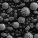
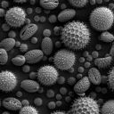
15.10	16.27	19.62	22.51	23.61	24.59	25.12	PSNR

Figure 6: Visual and numerical comparison of the recovered images, from noisy intensity-only coded diffraction pattern (CDP). The values denote the PSNR for each corresponding image. (Details are better appreciated on screen)

	$\alpha=9$	$\alpha=27$	$\alpha=81$
Algorithms	PSNR	PSNR	PSNR
HIO	35.96	25.76	14.82
WF	34.46	24.96	15.76
DOLPHIn	29.93	27.45	19.35
SPAR	35.20	31.82	22.44
BM3D-prGAMP	40.25	32.84	25.43
prDeep	39.70	33.54	26.82
Ours	40.33	33.90	27.23

Table 7: Quantitative comparison of different phase retrieval algorithms. The results are computed on four coded diffraction pattern measurements and varying the amount of Possion noise (a large $\alpha$ indicates low sigma-to-noise ratio). The best results are displayed in orange colour and the second best in blue colour.

4.5 Phase Retrieval

The goal of phase retrieval (PR) (Gerchberg, 1972) is to recover the underlying image from only the amplitude of the output of a complex linear system. It appears in many optical imaging applications, e.g., X-ray crystallography (Millane, 1990) and Fourier ptychography (Zheng et al., 2013). Mathematically, PR can be defined as the problem of recovering a signal $x\in\mathbb{R}^{N}$ or $\mathbb{C}^{N}$ from measurement $y$ of the form:

$$y=\sqrt{\left|Ax\right|^{2}+\omega},$$

where the measurement matrix $A$ represents the forward operator of the system, and $\omega$ represents shot noise. We approximate it with $\omega\sim\mathcal{N}(0,\alpha^{2}|Ax|^{2})$. The term $\alpha$ controls the sigma-to-noise ratio in this problem.

We test algorithms for phase retrieval with coded diffraction pattern (CDP) measurements (Candès et al., 2015). Multiple measurements with different random spatial modulator (SLM) patterns are recorded. We model the capture of four measurements using a phase-only SLM as (Metzler et al., 2018). Each measurement operator can be mathematically described as $A_{i}=\mathcal{F}D_{i},\quad i\in[1,2,3,4]$, where $\mathcal{F}$ can be represented by the 2D Fourier transform and $D_{i}$ is diagonal matrices with nonzero elements drawn uniformly from the unit circle in the complex planes.

We compare our method with three classic approaches (HIO (Fienup, 1982), WF (Candes et al., 2014), and DOLPHIn (Mairal et al., 2016)) and three PnP approaches (SPAR (Katkovnik, 2017), BM3D-prGAMP (Metzler et al., 2016a) and prDeep (Metzler et al., 2018)). Like CS-MRI and sparse-view CT applications, the parameters of these algorithms are carefully selected. Table 7 and Figure 6 summarize the results of all competing methods on twelve images used in (Metzler et al., 2018). It can be seen that our method still leads to state-of-the-art performance in this nonlinear inverse problem, and produces cleaner and clearer results than other competing methods.

5 Algorithm Investigation

In Section 4, we have shown the applications of our algorithms on both linear and nonlinear inverse imaging problems. We conduct more experiments to further investigate our TFPnP algorithm. We focus on four aspects of the algorithm: i) the choice of hyperparameters $m$, $N$ and $\eta$, ii) the relationship between the Gaussian denoising performance and the PnP performance, iii) the impact of auxiliary setting-related information feed into the policy, and iv) the behavior of the learned policy—how do the generated internal parameters (the denoising strength $\sigma_{k}$ and the penalty parameter $\mu_{k}$) look like? All experiments are carried out for the application of CS-MRI.

	$2\times$		$4\times$		$8\times$
($m$, $N$, $\eta$)	PSNR	#IT.	PSNR	#IT.	PSNR	#IT.
(3, 10, 0.05)	30.26	3.0	28.59	9.9	26.27	16.7
(10, 3, 0.05)	30.32	10.0	28.57	10.0	26.39	10.0
(5, 6, 0.05)	30.33	5.0	28.58	10.0	26.52	15.0
(5, 6, 0)	30.30	27.1	28.60	29.3	26.40	30.0
(5, 6, 0.1)	30.34	5.0	28.44	5.0	26.29	10.7
(5, 6, 0.25)	30.34	5.0	28.37	5.0	25.53	5.0

Table 8: Numerical comparison of the learned policies trained with different hyperparameters. The results are computed for the application of CS-MRI on seven medical images using undersampling factors of {2$\times$, 4$\times$, 8$\times$} and noise level of 15. The numerical values refer to the PSNR and the number of iterations (#IT.)

5.1 Hyperparameter Analysis

We discuss the choice of hyperparameters $m$, $N$ and $\eta$ in our TFPnP algorithm, where $m$ denotes the number of iterations of the optimization involved in the transition function $p$, $N$ is the maximum time step to run the policy, and $\eta$ sets the degree of penalty defined in the reward function. Table 8 shows the results of learned policies trained with different hyperparameter settings ($m$, $N$ and $\eta$) for CS-MRI. These results are divided into two groups (separated by the middle line) to analyze the effects of $(m,N)$ and $\eta$ respectively. Note that $N$ is varied with $m$ such that the maximum number of iterations $m\times N$ is fixed to 30 to keep comparisons fair. In the first group, we fix the value of $\eta$ and change the value of $m$. We observe all these settings yield similar results. It is up to users’ preference to choose $m$, where larger $m$ leads to coarser control of the termination time, but only requires fewer rounds of the decision making. In the second group, we keep $(m,N)$ constant while manipulating the value of $\eta$. We find $\eta$ serves as a key parameter to encourage early stopping. With $\eta=0$, the policy would not learn to early stop the optimization process, whilst large $\eta$ would make the policy stop too early.

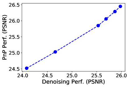
Figure 7: Performance (Perf.) behavior between Gaussian denoising and PnP-ADMM (with oracle policy) in terms of PSNR. The better the Gaussian denoiser the better the denoiser prior.

5.2 The Effect from the Gaussian Denoiser

To reveal the relationship between the Gaussian denoiser and the PnP performance, we train a set of denoising networks (U-net) with incremental Gaussian denoising performance (by adjusting the number of filters of networks). Then we incorporate these denoisers into the PnP-ADMM framework to evaluate their PnP performance on the CS-MRI application. The denoising strength/penalty parameters and the termination time are exhaustively searched to maximize PSNR to exclude the impact of internal parameters. Figure 7 clearly illustrates the positive correlation between the Gaussian denoising and PnP performance, indicating that a better Gaussian denoiser could serve as a better image prior when plugging into the PnP framework.

	$2\times$		$4\times$		$8\times$
	PSNR	#IT.	PSNR	#IT.	PSNR	#IT.
w/o extra info	30.15	27.4	28.36	29.1	26.27	30.0
+ “noise level”	30.31	9.1	28.53	15.0	26.34	21.4
+ “step”	30.29	10.0	28.48	17.5	26.37	23.6
Ours (full setting)	30.33	5.0	28.58	10.0	26.52	15.0

Table 9: Investigation of auxiliary setting-related information, i.e., the measurement noise level (denoted by ”noise level”) and the number of steps that have been taken so far (denoted by ”step”) encoded into the policy network. The results are evaluated on CS-MRI with speed-up of {2$\times$, 4$\times$, 8$\times$} and noise level of 15.

5.3 The Effect from Auxiliary Setting-related Information

Our policy network makes use of auxiliary setting-related information (i.e., the measurement noise level, and the number of steps that has been taken) encoded as additional input feature planes to learn a problem-aware policy. To analyze its impact, we train policy networks without or with partial auxiliary information. As shown in Table 9, by encoding these setting-related quantities, the policy network learns to be aware of the problem settings, thus deriving a better parameter-tuning policy with faster convergence and higher accuracy.

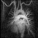
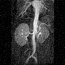
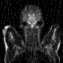
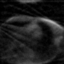
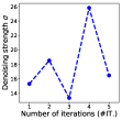
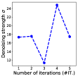
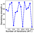
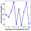
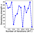
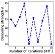
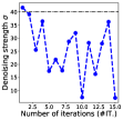
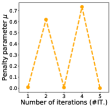
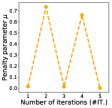
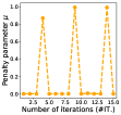
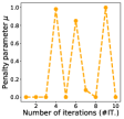
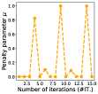
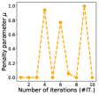
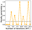
Figure 8: Behavior curves of our learned policy for the application of CS-MRI reconstruction on medical images. The first row displays the initial estimate $x_{0}$ of the underlying image. The second row shows the predicted denoising strength, $\sigma$, computed by our learned policy for each corresponding image. The third row displays the predicted penalty parameters $\mu$ vs the number of iterations.

5.4 Behaviors of Learned Policy

To visualize the behavior of our learned policy towards different images, we illustrate its generated parameters ($\sigma_{k}$ and $\mu_{k}$) along iterations in Figure 8. It can be observed that our learned policy customizes different internal parameters for each different image, whilst the generated parameters change adaptively across iterations of the optimization process. The adaptive penalization has been justified to result in faster convergence in the convex setting both empirically and theoretically (Xu et al., 2017b, a, c; Goldstein et al., 2015; He et al., 2000). We conjecture similar result holds for the nonconvex setting as well, where the underlying adaptive parameter scheme can be automatically mined by our algorithm from the data, leading to a more efficient and effective policy than the oracle one.

	PnP-PGM		PnP-APGM		PnP-HQS		RED-ADMM		PnP-ADMM
Policies	PSNR	#IT.	PSNR	#IT.	PSNR	#IT.	PSNR	#IT.	PSNR	#IT.
fixed	24.98	30.0	24.39	30.0	24.82	30.0	24.57	30.0	22.78	30.0
fixed∗	24.99	20.9	25.07	13.6	24.83	20.6	24.58	27.3	24.19	7.3
fixed optimal	25.66	30.0	24.73	30.0	25.27	30.0	25.14	30.0	26.08	30.0
fixed optimal∗	25.68	21.1	25.69	11.4	25.35	27.6	25.15	29.1	26.16	16.7
greedy	24.83	30.0	24.46	30.0	24.34	30.0	24.95	30.0	26.20	30.0
greedy∗	25.21	15.8	25.04	9.3	24.35	22.9	25.44	19.0	26.33	19.0
oracle	25.85	30.0	25.21	30.0	25.50	30.0	25.36	30.0	26.41	30.0
oracle∗	25.90	21.4	25.87	11.9	25.55	24.6	25.45	27.8	26.45	21.6
Ours	26.28	20.7	26.36	10.0	25.96	22.2	26.11	22.1	26.52	15.0

Table 10: Comparisons of different PnP-type algorithms using different policies for CS-MRI reconstruction (* denotes the policies with optimal early stopping). The maximum number of iteration is set as 30 for policies without early stopping. The results are computed on seven medical images using an acceleration factor of 8$\times$ and a noise level of 15. The numerical values reflect the PSNR and number of iterations (#IT.). The best and the second best results among policies within the same category of the PnP-type algorithm (the best results in each column) are displayed in orange and blue colors respectively, and the best results among all PnP-type algorithms using the same policy (the best result in each row) are underlined.

	$2\times$		$4\times$		$8\times$
D-AMP	PSNR	#IT.	PSNR	#IT.	PSNR	#IT.
original	29.49	30.0	28.12	30.0	26.02	30.0
original∗	29.51	6.3	28.13	9.7	26.09	17.1
Ours	30.31	5.0	28.55	10.7	26.49	14.3

Table 11: Numerical comparison (PSNR / #IT.) of original D-AMP (* denotes optimal early stopping) and D-AMP with our learned policy for CS-MRI under various acceleration factors ($2\times$,$4\times$,$8\times$) with noise level 15.

6 Extensions to Other PnP-type Algorithms

In previous sections, we have provided extensive experiments to demonstrate the efficiency of our proposed algorithmic approach, instantiated by PnP-ADMM, on several inverse imaging problems. In this section, we show that the advantages of our approach hold for other PnP-type algorithms as well. We remark that the extensions of our approach to other proximal algorithms are straightforward and flexible, i.e., one only needs to adjust the desired outputs of the policy network (the number of internal parameters) to match the corresponding PnP algorithms. In what follows, we detail the extensions on five representative PnP-type algorithms—PnP-PGM/APGM (Sun et al., 2019b), PnP-HQS (Zhang et al., 2017b), RED-ADMM (Romano et al., 2017), D-AMP (Metzler et al., 2016b), and comprehensively study their performance on the CS-MRI application.

6.1 Other PnP-type Algorithms

PnP-PGM/APGM

We first introduce the formulation of PnP proximal gradient method (PGM) and its accelerated variant (APGM). Both of them can be expressed in an unified manner as follows:

$$\begin{split}&z_{k+1}=s_{k}-\gamma_{k}\nabla\mathcal{D}(s_{k}),\\ &x_{k+1}=\mathrm{Prox}_{\sigma_{k}^{2}\mathcal{R}}(z_{k+1})=\mathcal{H}_{\sigma_{k}}(z_{k+1}),\\ &s_{k+1}=x_{k+1}+\frac{q_{k}-1}{q_{k+1}}(x_{k+1}-x_{k}),\end{split}$$ (19)

where $\gamma_{k}$ denotes the step size for the gradient descent of the data-fidelity term. $q_{k}$ is an intermediate parameter for computing inertial parameter. If $q_{k}=1$ and its update follows:

$$q_{k+1}=\frac{1}{2}\big{(}1+\sqrt{1+4q_{k}^{2}}\big{)},$$

the algorithm (19) corresponds to APGM (or FISTA) (Beck and Teboulle, 2009). When $q_{k}\equiv 1$, then $s_{k}=x_{k}$ and (19) recovers the standard PGM.

The fundamental conceptual differences between PGM and ADMM lie at their treatment of the data-fidelity $\mathcal{D}$. To ensure data consistency, PGM adopts a simple gradient descent with step size $\gamma_{k}$, while ADMM relies on the proximal operator $\mathrm{Prox}_{\frac{1}{\mu_{k}}\mathcal{D}}$ with penalty parameter $\mu_{k}$. This leads to the different forms of internal parameters. Therefore, to adapt our algorithm into PnP-PGM, we modify the policy network to determine the step size $\gamma_{k}$, in place of the penalty parameter $\mu_{k}$. For PnP-APGM, we treat $\bar{q_{k}}:=\frac{q_{k}-1}{q_{k+1}}$ as an additional parameter and learn to predict $\bar{q_{k}}$ using the policy network.

PnP-HQS

Next, we introduce the PnP half quadratic splitting (HQS) algorithm, formulated as:

$$\begin{split}&x_{k+1}=\mathrm{Prox}_{\sigma_{k}^{2}\mathcal{R}}\left(z_{k}\right)=\mathcal{H}_{\sigma_{k}}\left(z_{k}\right),\\ &z_{k+1}=\mathrm{Prox}_{\frac{1}{\mu_{k}}\mathcal{D}}\left(x_{k+1}\right),\\ \end{split}$$ (20)

Roughly speaking, HQS can be viewed as a simplified version of ADMM. The only difference is that HQS does not have the dual variable $u$ (or $u$ is set to zero constantly), and the internal parameters of PnP-HQS conform with those of PnP-ADMM. As a result, no modification is required to learn a policy customized for PnP-HQS.

RED-ADMM

Then, we show our algorithm can be used in another PnP-type framework, namely regularization by denoising (RED) as well. Unlike the PnP with implicit prior characterized by the PnP denoiser, the RED formulates an explicit prior term involving an denoising engine:

$$\mathcal{R}\left(x\right)=\frac{1}{2}x^{T}\left(x-\mathcal{H}_{\sigma}\left(x\right)\right),$$ (21)

in which the denoising engine itself is applied on the candidate image $x$, and the penalty induced is proportional to the inner product between this image and its denoising residual, $x-\mathcal{H}_{\sigma}\left(x\right)$. Under some assumptions on $\mathcal{H}\left(\cdot\right)$, the gradient of the regularization term is manageable (Romano et al., 2017). As a result, the resulted objective function can be solved by proper numerical schemes, e.g., gradient descent, ADMM or fixed-point strategy. For simplicity, we choose the inexact RED-ADMM with one fixed-point iteration as a proof-of-concept, which is given by

$$\begin{split}&v_{k+1}=\mathcal{H}_{\sigma_{k}}\left(x_{k}\right),\\ &x_{k+1}=\tfrac{1}{\mu_{k}+\lambda_{k}}\big{(}\lambda_{k}v_{k+1}+\mu_{k}(z_{k}-u_{k})\big{)},\\ &z_{k+1}=\mathrm{Prox}_{\frac{1}{\mu_{k}}\mathcal{D}}\left(x_{k+1}+u_{k}\right),\\ &u_{k+1}=u_{k}+x_{k+1}-z_{k+1}.\end{split}$$ (22)

Compared to PnP-ADMM, we modify our policy network and incorporate $\lambda_{k}$ into our parameter prediction.

D-AMP

Finally, we present our algorithmic approach on the denoising-based approximate message passing (D-AMP) framework. Different from proximal algorithms developed in optimization community, the AMP algorithm is initially derived from the loopy belief propagation in graphical models from Bayesian statistics community (Donoho et al., 2009). One form of AMP algorithm reads

$$\begin{split}&v_{k+1}=x_{k}+\mathcal{A}^{H}z_{k},\\ &x_{k+1}=f\left(v_{k+1}\right),\\ &o_{k+1}=\frac{1}{M}z_{k}\mathop{\mathrm{Div}}\{f\left(v_{k+1}\right)\},\\ &z_{k+1}=y-\mathcal{A}x_{k+1}+o_{k+1},\end{split}$$ (23)

where $\mathcal{A}^{H}:\mathbb{R}^{M}\to\mathbb{R}^{N}$ or $\mathbb{C}^{M}\to\mathbb{C}^{N}$ is the adjoint operator for the forward operator $\mathcal{A}$, and $\mathop{\mathrm{Div}}\{f(v)\}$ denotes the divergence (i.e., the summation of derivatives) of an operator $f$ with respect to its input $v$. In the original form of AMP, $f$ is a shrinkage/thresholding non-linearity, which can be replaced by a proper denoiser $\mathcal{H}_{\sigma_{k}}$ demonstrated in D-AMP framework. For complicated denoisers without analytical form of divergence, the divergence is approximated by the Monte Carlo method (Ramani et al., 2008). One distinguishing feature of AMP algorithms is the Onsager correction term $o_{k}$, which renders the effective noise define by $v_{k}-x$ approximately Gaussian, and thus the noise level of effective noise at each iteration can be estimated via

$$\hat{\sigma}_{k+1}=\frac{\|z_{k}\|_{2}}{\sqrt{M}},$$ (24)

This quantity can be used to adaptively set the denoising strength $\sigma_{k}$ of the employed denoiser in an automated manner. However, the above property of AMP only holds for compressed sensing applications with i.i.d. sub-Gaussian measurement matrices. Even though it has been extended to handle larger classes of random matrices, (Cakmak et al., 2014; Manoel et al., 2015; Ma and Ping, 2017; Rangan et al., 2019a, b; Millard et al., 2020; Metzler and Wetzstein, 2021), the behavior of AMP under general $\mathcal{A}$ is largely unpredictable and may even diverge in many situations where the internal parameters are not properly chosen. Here, we show our automated parameter tuning scheme is also effective to tackle this dilemma by predicting the denoising strength at D-AMP iteration using our learned policy. Instead of directly inferring $\sigma_{k}$, we make full use of the initial estimate of (24) and introduce a multiplicative factor $\delta$ into it, thereby the final $\sigma_{k}=\delta\hat{\sigma}_{k}$. The policy network is thus responsible for predicting $\delta$ from data.

Result Analysis

With these simple modifications at hand, our algorithm can be readily applied to these PnP-type algorithms to learn their tailored policies. Moreover, we also evaluate the other policies defined in Section 4.2. Table 10 and Table 11 summarize the numerical results of different PnP-type algorithms equipped with different policies, from which we observed that our learned policy can produce extremely effective parameters for these PnP-type algorithms and consistently outperforms the oracle policies. Note that, PnP-ADMM is still the top-performing PnP-type algorithm, while PnP-APGM with our learned policy can reach a comparable performance using fewer iterations. These results collectively show the adaptive parameter scheme (yielded by our learned policy) is of great benefit to PnP-type algorithms, with regard to both practical convergence and restoration accuracy.

	PnP-PGM	PnP-APGM	PnP-HQS	PnP-ADMM
IT#1
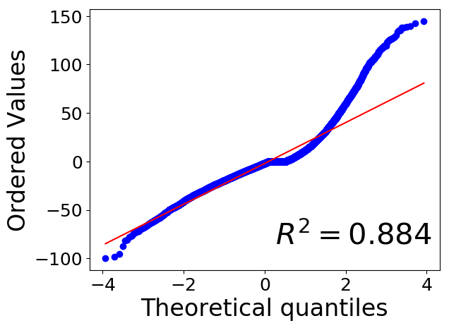
IT#2
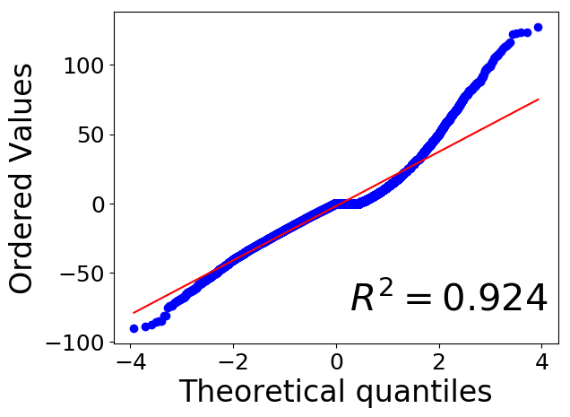
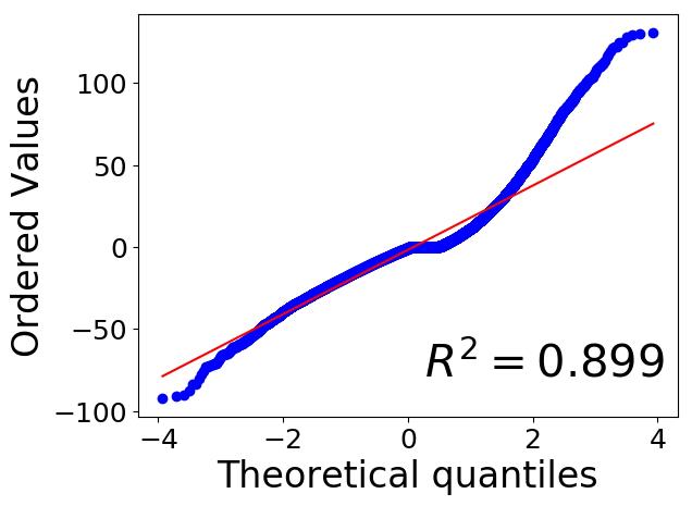
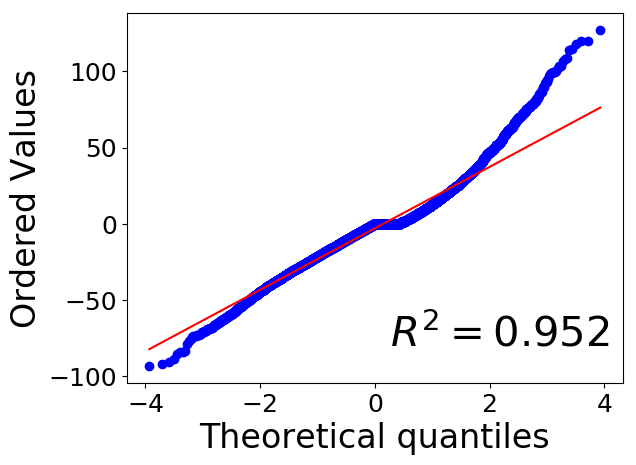
IT#3
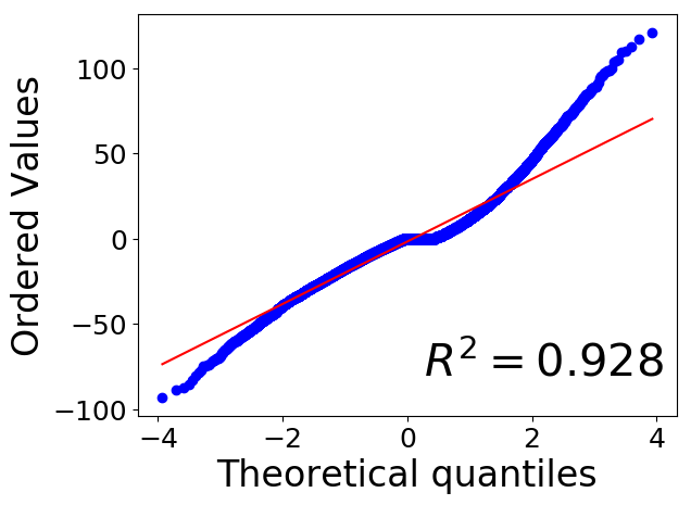
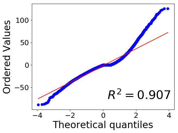
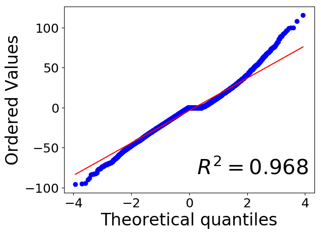
IT#30

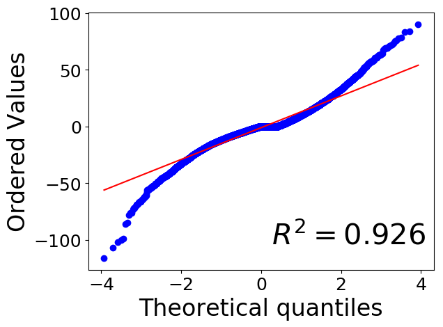
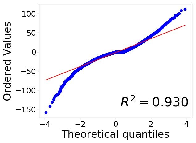
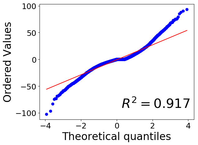
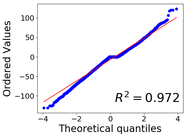
Figure 9: Gaussian probability plots of iteration noise at four specific iterations (#1, #2, #3 and #30) for different PnP algorithms with oracle policies. The resulting image looks close to a straight line if the data are approximately Gaussian distributed. A higher $R^{2}$ indicates a better fit.

Fixed Policy
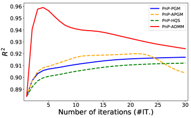
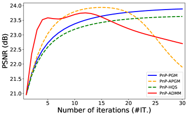
Oracle Policy
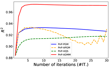
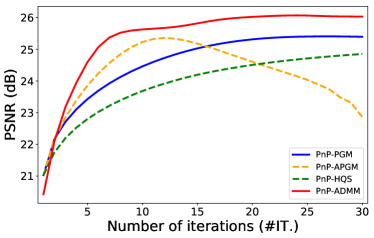
Learned Policy

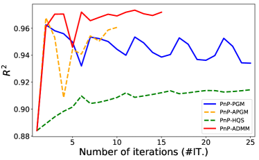
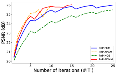
Figure 10: $R^{2}$ curve (Left) and PSNR curve (Right) across iterations for four PnP algorithms using three different policies.

6.2 Iteration Noise of PnP Methods

The promising results reported in Table 10 push us to further think of a puzzling question—Why are there distinctions among different PnP algorithms regarding recovery performance, especially given the fact that these PnP algorithms share the same set of fixed points? Directly answering this question could be rather difficult, but fortunately, we find some clues that could be potentially useful to analyze the performance of different PnP methods. To do this, we leverage a concept called iteration noise, which can characterize the statistical property of PnP algorithms and shed light on the explanation of the aforementioned question.

For all PnP algorithms, the key step is the denoising step using the PnP prior, which is

$$x_{k+1}=\mathrm{Prox}_{\sigma_{k}^{2}\mathcal{R}}(\bar{x}_{k})=\mathcal{H}_{\sigma_{k}}(\bar{x}_{k}),$$ (25)

where $x_{k}$ is the recovered image by the algorithm at the $k$-th iteration, $\bar{x}_{k}$ is the intermediate variable whose form depends on the given PnP algorithm. For instance, we have $\bar{x}_{k}:=z_{k}-u_{k}$ in PnP-ADMM.

Typically, the PnP denoiser $\mathcal{H}_{\sigma_{k}}$ is designed or trained for the purpose of Gaussian denoising (Venkatakrishnan et al., 2013), given the proximal operator $\mathrm{Prox}_{\sigma_{k}^{2}\mathcal{R}}$ sets up a regularized Gaussian denoising problem. Such a denoiser is most desired and effective for removing Gaussian noise, but its performance would be severely degraded when tackling with other non-Gaussian noise (Plotz and Roth, 2017; Wei et al., 2020b). In this regard, investigating the noise the PnP denoiser intends to suppress, serves as an important clue to analyze the performance of PnP methods. To facilitate further analysis, let $x$ be the underlying image that we want to recover, then we can rewrite (25) to

$$x_{k+1}=\mathcal{H}_{\sigma_{k}}(x+\bar{x}_{k}-x)=\mathcal{H}_{\sigma_{k}}(x+\epsilon_{k}),$$ (26)

where $\epsilon_{k}=\bar{x}_{k}-x$ measures the discrepancy between the current estimate $\bar{x}_{k}$ and the ground truth $x$ at $k$-th iteration. We term this quantity as the iteration noise of the PnP algorithm in the $k$-th iteration. It should be acknowledged the similar quantity has been called by effective noise in the context of D-AMP algorithm (Metzler et al., 2016b), but here we elaborate more on its characteristics varying along iterations, in the broader context of general PnP framework.

Ideally, the PnP denoiser should be designed/trained for removing the iteration noise $\varepsilon_{k}$. However, it is unclear what probability distributions $\varepsilon_{k}$ complies in practice, as it can vary across different inverse imaging applications, different proximal algorithms, as well as different internal parameter settings. Without any prior information available in advance, we argue that the Gaussian denoiser is still the most universal choice for the PnP algorithm given the central limit theorem.

Although theoretical justifications of the iteration noise are highly difficult, we can provide empirical analysis on it in the context of PnP methods with Gaussian denoiser. Intuitively, the performance of PnP methods relies on the effectiveness of the PnP denoiser to remove the iteration noise. The more the iteration noise resembles the Gaussian noise, the more likely it can be suppressed by the Gaussian denoiser. To test the normality of the iteration noise, we employ the Gaussian probability plot (Wilk and Gnanadesikan, 1968) on the iteration noise for different PnP algorithms with oracle policies. We also evaluate the goodness-of-fit by $R^{2}$—the coefficient of determination with respect to the resulting probability plot (Morgan et al., 2011). The obtained results are shown in Figure 9, from which we observe that: 1) for all PnP algorithms, their corresponding iteration noise shows heavy tails in the beginning stage of the iteration; 2) the degrees of heavy tails are alleviated along iterations for all algorithms and 3) PnP-ADMM shows the best improvement over the other three—it improves the $R^{2}$ to 0.972, whilst the best value from the other three is 0.930 from PnP-APGM. This also conforms with the performance shown in Table 10, where PnP-ADMM performs favorably against others in the oracle policy setting (e.g., 26.41 for PnP-ADMM, 25.85 for PnP-PGM).

To conclude this discussion, we display in Figure 10 that $R^{2}$ and PSNR vary over iterations for all PnP methods armed with three policies (i.e., fixed policy, oracle policy, and learned policy). It can be seen that compared to the oracle policy, the normality of iteration noise and the recovery performance of PnP-type algorithms (e.g., PnP-APGM/PGM) can be significantly improved with our learned policy. It also implies a positive correlation between $R^{2}$ and PSNR values, suggesting the benefit of Gaussianizing iteration noise. We note the importance of Gaussianizing iteration noise has been demonstrated from the AMP literature. In fact, much of the success of AMP is directly attributed to the Gaussian distribution of iteration noise (Donoho et al., 2009). Here, we generalize this conclusion beyond the scope of AMP, to the wide spectrum of PnP methods.

7 Conclusion and Future Works

In this work, we introduced reinforcement learning (RL) into the PnP framework, yielding a novel tuning-free PnP proximal algorithm for a wide range of inverse imaging problems. The main strength of our approach is the policy network, which can customize parameters for different images. Through numerical experiments, we demonstrate our learned policy often generates highly effective parameters, which often even reaches comparable performance to the “oracle” parameters tuned towards the ground truth.

Our approach takes a big step towards solving the issues of tuning and slow-convergence, known weaknesses of PnP-type methods. There is, however, still room left for improvement. For example, our proposed algorithm relies on a mixture of a model-free and a model-based RL algorithm for learning the policy network. We believe that recently proposed more advanced RL algorithms can be adopted to our framework and further boost the performance of the learned policy. Moreover, the current version of our algorithm can only scale to moderately-sized imaging problems. Making it scalable to large-scale settings is a non-trivial task left for future research. Last but not least, our empirical analysis of the iteration noise reveals some hidden structures of PnP proximal algorithms. Seeking a deep understanding of what makes these algorithms stand out in terms of performance is an interesting and challenging question. We foresee a rich pool of future research to further tackle these challenges, aiming at efficient, effective, and versatile image recovery for inverse imaging applications.

Acknowledgments

This research was supported by the National Natural Science Foundation of China under Grant No. 62171038, No. 61827901, No. 61936011, and No. 62088101. Authors also gratefully acknowledge the financial support of the CMIH and CCIMI University of Cambridge, and Graduate school of Beijing Institute of Technology. AIAR gratefully acknowledges the financial support of the CMIH and CCIMI University of Cambridge. JL acknowledges support from the Leverhulme Trust, Shanghai Municipal Science and Technology Major Project (2021SHZDZX0102). CBS acknowledges support from the Philip Leverhulme Prize, the Royal Society Wolfson Fellowship, the EPSRC grants EP/S026045/1 and EP/T003553/1, EP/N014588/1, EP/T017961/1, the Wellcome Innovator Award RG98755, the Leverhulme Trust project Unveiling the invisible, the European Union Horizon 2020 research and innovation programme under the Marie Skodowska-Curie grant agreement No. 777826 NoMADS, the Cantab Capital Institute for the Mathematics of Information and the Alan Turing Institute.

References

- Adler and Oktem (2018) J. Adler and O. Oktem. Learned primal-dual reconstruction. IEEE Transactions on Medical Imaging, 37(6):1322–1332, 2018.
- Aggarwal and Jacob (2020) H. K. Aggarwal and M. Jacob. J-modl: Joint model-based deep learning for optimized sampling and reconstruction. IEEE Journal of Selected Topics in Signal Processing, 14(6):1151–1162, 2020.
- Aggarwal et al. (2018) H. K. Aggarwal, M. P. Mani, and M. Jacob. Modl: Model-based deep learning architecture for inverse problems. IEEE Transactions on Medical Imaging, 38(2):394–405, 2018.
- Aguet et al. (2008) F. Aguet, D. Van De Ville, and M. Unser. Model-based 2.5-d deconvolution for extended depth of field in brightfield microscopy. IEEE Transactions on Image Processing, 17(7):1144–1153, 2008.
- Alver et al. (2020) M. B. Alver, A. Saleem, and M. Çetin. Plug-and-play synthetic aperture radar image formation using deep priors. IEEE Transactions on Computational Imaging, 7:43–57, 2020.
- Arridge et al. (2019) S. Arridge, P. Maass, O. Öktem, and C.-B. Schönlieb. Solving inverse problems using data-driven models. Acta Numerica, 28:1–174, 2019.
- Bauschke et al. (2011) H. H. Bauschke, P. L. Combettes, et al. Convex analysis and monotone operator theory in Hilbert spaces, volume 408. Springer, 2011.
- Bayati and Montanari (2011) M. Bayati and A. Montanari. The dynamics of message passing on dense graphs, with applications to compressed sensing. IEEE Transactions on Information Theory, 57(2):764–785, 2011.
- Bayati et al. (2013) M. Bayati, M. A. Erdogdu, and A. Montanari. Estimating lasso risk and noise level. In Advances in Neural Information Processing Systems, volume 26, pages 944–952, 2013.
- Beck and Teboulle (2009) A. Beck and M. Teboulle. A fast iterative shrinkage-thresholding algorithm for linear inverse problems. SIAM Journal on Imaging Sciences, 2(1):183–202, 2009.
- Benning and Burger (2018) M. Benning and M. Burger. Modern regularization methods for inverse problems. arXiv preprint arXiv:1801.09922, 2018.
- Blu and Luisier (2007) T. Blu and F. Luisier. The sure-let approach to image denoising. IEEE Transactions on Image Processing, 16(11):2778–2786, 2007.
- Boyd et al. (2011) S. Boyd, N. Parikh, E. Chu, B. Peleato, J. Eckstein, et al. Distributed optimization and statistical learning via the alternating direction method of multipliers. Foundations and Trends® in Machine learning, 3(1):1–122, 2011.
- Brifman et al. (2016) A. Brifman, Y. Romano, and M. Elad. Turning a denoiser into a super-resolver using plug and play priors. In IEEE International Conference on Image Processing, pages 1404–1408. IEEE, 2016.
- Brifman et al. (2019) A. Brifman, Y. Romano, and M. Elad. Unified single-image and video super-resolution via denoising algorithms. IEEE Transactions on Image Processing, 28(12):6063–6076, 2019.
- Brooks et al. (2019) T. Brooks, B. Mildenhall, T. Xue, J. Chen, D. Sharlet, and J. T. Barron. Unprocessing images for learned raw denoising. In IEEE Conference on Computer Vision and Pattern Recognition, pages 11036–11045, 2019.
- Buades et al. (2005) A. Buades, B. Coll, and J.-M. Morel. A non-local algorithm for image denoising. In IEEE Conference on Computer Vision and Pattern Recognition, pages 60–65, 2005.
- Buzzard et al. (2018) G. T. Buzzard, S. H. Chan, S. Sreehari, and C. A. Bouman. Plug-and-play unplugged: Optimization-free reconstruction using consensus equilibrium. SIAM Journal on Imaging Sciences, 11(3):2001–2020, 2018.
- Cakmak et al. (2014) B. Cakmak, O. Winther, and B. H. Fleury. S-amp: Approximate message passing for general matrix ensembles. In IEEE Information Theory Workshop, pages 192–196. IEEE, 2014.
- Candes et al. (2014) E. Candes, X. Li, and M. Soltanolkotabi. Phase retrieval via wirtinger flow: Theory and algorithms. IEEE Transactions on Information Theory, 61(4):1985–2007, 2014.
- Candès et al. (2015) E. J. Candès, X. Li, and M. Soltanolkotabi. Phase retrieval from coded diffraction patterns. Applied and Computational Harmonic Analysis, 39(2):277–299, 2015.
- Chambolle and Pock (2011) A. Chambolle and T. Pock. A first-order primal-dual algorithm for convex problems with applications to imaging. Journal of Mathematical Imaging and Vision, 40(1):120–145, 2011.
- Chambolle and Pock (2016) A. Chambolle and T. Pock. An introduction to continuous optimization for imaging. Acta Numerica, 25:161–319, 2016.
- Chan (2019) S. H. Chan. Performance analysis of plug-and-play admm: A graph signal processing perspective. IEEE Transactions on Computational Imaging, 5(2):274–286, 2019.
- Chan and Lu (2014) S. H. Chan and Y. M. Lu. Efficient image reconstruction for gigapixel quantum image sensors. In IEEE Global Conference on Signal and Information Processing, pages 312–316. IEEE, 2014.
- Chan et al. (2017) S. H. Chan, X. Wang, and O. A. Elgendy. Plug-and-play admm for image restoration: Fixed-point convergence and applications. IEEE Transactions on Computational Imaging, 3(1):84–98, 2017.
- Chen et al. (2017) H. Chen, Y. Zhang, M. K. Kalra, F. Lin, Y. Chen, P. Liao, J. Zhou, and G. Wang. Low-dose ct with a residual encoder-decoder convolutional neural network. IEEE transactions on medical imaging, 36(12):2524–2535, 2017.
- Chen et al. (2021) T. Chen, X. Chen, W. Chen, H. Heaton, J. Liu, Z. Wang, and W. Yin. Learning to optimize: A primer and a benchmark. arXiv preprint arXiv:2103.12828, 2021.
- Chun et al. (2019) I. Y. Chun, Z. Huang, H. Lim, and J. A. Fessler. Momentum-net: Fast and convergent iterative neural network for inverse problems. arXiv preprint arXiv:1907.11818, 2019.
- Cohen et al. (2020) R. Cohen, M. Elad, and P. Milanfar. Regularization by denoising via fixed-point projection (red-pro). arXiv preprint arXiv:2008.00226, 2020.
- Dabov et al. (2007) K. Dabov, A. Foi, V. Katkovnik, and K. Egiazarian. Image denoising by sparse 3-d transform-domain collaborative filtering. IEEE Transactions on Image Processing, 16(8):2080, 2007.
- Danielyan et al. (2010) A. Danielyan, V. Katkovnik, and K. Egiazarian. Image deblurring by augmented lagrangian with bm3d frame prior. In Workshop on Information Theoretic Methods in Science and Engineering, pages 16–18, 2010.
- Dar et al. (2016) Y. Dar, A. M. Bruckstein, M. Elad, and R. Giryes. Postprocessing of compressed images via sequential denoising. IEEE Transactions on Image Processing, 25(7):3044–3058, 2016.
- Daubechies (1992) I. Daubechies. Ten lectures on wavelets. SIAM, 1992.
- Daubechies et al. (2004) I. Daubechies, M. Defrise, and C. De Mol. An iterative thresholding algorithm for linear inverse problems with a sparsity constraint. Communications on Pure and Applied Mathematics: A Journal Issued by the Courant Institute of Mathematical Sciences, 57(11):1413–1457, 2004.
- Diamond et al. (2017) S. Diamond, V. Sitzmann, F. Heide, and G. Wetzstein. Unrolled optimization with deep priors. arXiv preprint arXiv:1705.08041, 2017.
- Dong et al. (2018) W. Dong, P. Wang, W. Yin, G. Shi, F. Wu, and X. Lu. Denoising prior driven deep neural network for image restoration. IEEE Transactions on Pattern Analysis and Machine Intelligence, 41(10):2305–2318, 2018.
- Dong et al. (2021) W. Dong, C. Zhou, F. Wu, J. Wu, G. Shi, and X. Li. Model-guided deep hyperspectral image super-resolution. IEEE Transactions on Image Processing, 2021.
- Donoho and Johnstone (1995) D. L. Donoho and I. M. Johnstone. Adapting to unknown smoothness via wavelet shrinkage. Journal of the American Statistical Association, 90(432):1200–1224, 1995.
- Donoho et al. (2009) D. L. Donoho, A. Maleki, and A. Montanari. Message-passing algorithms for compressed sensing. Proceedings of the National Academy of Sciences, 106(45):18914–18919, 2009.
- Donoho et al. (2010a) D. L. Donoho, A. Maleki, and A. Montanari. Message passing algorithms for compressed sensing: I. motivation and construction. In IEEE information theory workshop on information theory, pages 1–5. IEEE, 2010a.
- Donoho et al. (2010b) D. L. Donoho, A. Maleki, and A. Montanari. Message passing algorithms for compressed sensing: Ii. analysis and validation. In IEEE Information Theory Workshop on Information Theory, pages 1–5. IEEE, 2010b.
- Eckstein and Bertsekas (1992) J. Eckstein and D. P. Bertsekas. On the douglas—rachford splitting method and the proximal point algorithm for maximal monotone operators. Mathematical Programming, 55(1-3):293–318, 1992.
- Eksioglu (2016) E. M. Eksioglu. Decoupled algorithm for mri reconstruction using nonlocal block matching model: Bm3d-mri. Journal of Mathematical Imaging and Vision, 56(3):430–440, 2016.
- Eksioglu and Tanc (2018) E. M. Eksioglu and A. K. Tanc. Denoising amp for mri reconstruction: Bm3d-amp-mri. SIAM Journal on Imaging Sciences, 11(3):2090–2109, 2018.
- Elbakri and Fessler (2002) I. A. Elbakri and J. A. Fessler. Segmentation-free statistical image reconstruction for polyenergetic x-ray computed tomography. In IEEE International Symposium on Biomedical Imaging, pages 828–831, 2002.
- Eldar (2008) Y. C. Eldar. Generalized sure for exponential families: Applications to regularization. IEEE Transactions on Signal Processing, 57(2):471–481, 2008.
- Engl et al. (1996) H. W. Engl, M. Hanke, and A. Neubauer. Regularization of inverse problems, volume 375. Springer Science & Business Media, 1996.
- Esser et al. (2010) E. Esser, X. Zhang, and T. F. Chan. A general framework for a class of first order primal-dual algorithms for convex optimization in imaging science. SIAM Journal on Imaging Sciences, 3(4):1015–1046, 2010.
- Everingham et al. (2014) M. Everingham, S. Eslami, L. Van Gool, C. Williams, J. Winn, and A. Zisserman. The pascal visual object classes challenge: A retrospective. International Journal of Computer Vision, 111, 01 2014.
- Fazel et al. (2001) M. Fazel, H. Hindi, and S. P. Boyd. A rank minimization heuristic with application to minimum order system approximation. In Proceedings of the American Control Conference, volume 6, pages 4734–4739. IEEE, 2001.
- Fessler (2010) J. A. Fessler. Model-based image reconstruction for mri. IEEE Signal Processing Magazine, 27(4):81–89, 2010.
- Fienup (1982) J. R. Fienup. Phase retrieval algorithms: a comparison. Applied Optics, 21(15):2758–2769, 1982.
- Fossum (2011) E. R. Fossum. The quanta image sensor (qis): concepts and challenges. In Imaging Systems and Applications, page JTuE1. Optical Society of America, 2011.
- Fossum et al. (2016) E. R. Fossum, J. Ma, S. Masoodian, L. Anzagira, and R. Zizza. The quanta image sensor: Every photon counts. Sensors, 16(8):1260, 2016.
- Furuta et al. (2019) R. Furuta, N. Inoue, and T. Yamasaki. Fully convolutional network with multi-step reinforcement learning for image processing. In AAAI Conference on Artificial Intelligence, pages 3598–3605, 2019.
- Gabay and Mercier (1976) D. Gabay and B. Mercier. A dual algorithm for the solution of nonlinear variational problems via finite element approximation. Computers & mathematics with applications, 2(1):17–40, 1976.
- Gavaskar et al. (2021) R. G. Gavaskar, C. D. Athalye, and K. N. Chaudhury. On plug-and-play regularization using linear denoisers. IEEE Transactions on Image Processing, 30:4802–4813, 2021.
- Geman (1995) D. Geman. Nonlinear image recovery with half-quadratic regularization. IEEE Transactions on Image Processing, 4(7):932–946, 1995.
- Gerchberg (1972) R. W. Gerchberg. A practical algorithm for the determination of phase from image and diffraction plane pictures. Optik, 35:237–246, 1972.
- Gilton et al. (2019) D. Gilton, G. Ongie, and R. Willett. Neumann networks for linear inverse problems in imaging. IEEE Transactions on Computational Imaging, 6:328–343, 2019.
- Giryes et al. (2008) R. Giryes, M. Elad, and Y. C. Eldar. Automatic parameter setting for iterative shrinkage methods. In IEEE Convention of Electrical and Electronics Engineers in Israel, pages 820–824. IEEE, 2008.
- Giryes et al. (2011) R. Giryes, M. Elad, and Y. C. Eldar. The projected gsure for automatic parameter tuning in iterative shrinkage methods. Applied and Computational Harmonic Analysis, 30(3):407–422, 2011.
- Goldstein et al. (2015) T. Goldstein, M. Li, and X. Yuan. Adaptive primal-dual splitting methods for statistical learning and image processing. In Advances in Neural Information Processing Systems, pages 2089–2097. 2015.
- Golub et al. (1979) G. H. Golub, M. Heath, and G. Wahba. Generalized cross-validation as a method for choosing a good ridge parameter. Technometrics, 21(2):215–223, 1979.
- Gregor and LeCun (2010) K. Gregor and Y. LeCun. Learning fast approximations of sparse coding. In International Conference on Machine Learning, pages 399–406, 2010.
- Gu et al. (2017) S. Gu, Q. Xie, D. Meng, W. Zuo, X. Feng, and L. Zhang. Weighted nuclear norm minimization and its applications to low level vision. International Journal of Computer Vision, 121(2):183–208, 2017.
- Guo and Davies (2015) C. Guo and M. E. Davies. Near optimal compressed sensing without priors: Parametric sure approximate message passing. IEEE Transactions on Signal Processing, 63(8):2130–2141, 2015.
- Gupta et al. (2018) H. Gupta, K. H. Jin, H. Q. Nguyen, M. T. McCann, and M. Unser. Cnn-based projected gradient descent for consistent ct image reconstruction. IEEE transactions on medical imaging, 37(6):1440–1453, 2018.
- Hansen (1992) P. C. Hansen. Analysis of discrete ill-posed problems by means of the l-curve. SIAM Review, 34(4):561–580, 1992.
- Hansen (1999) P. C. Hansen. The l-curve and its use in the numerical treatment of inverse problems. 1999.
- Hansen and O’Leary (1993) P. C. Hansen and D. P. O’Leary. The use of the l-curve in the regularization of discrete ill-posed problems. SIAM Journal on Scientific Computing, 14(6):1487–1503, 1993.
- He et al. (2000) B. He, H. Yang, and S. Wang. Alternating direction method with self-adaptive penalty parameters for monotone variational inequalities. Journal of Optimization Theory and applications, 106(2):337–356, 2000.
- He et al. (2018) J. He, Y. Yang, Y. Wang, D. Zeng, Z. Bian, H. Zhang, J. Sun, Z. Xu, and J. Ma. Optimizing a parameterized plug-and-play admm for iterative low-dose ct reconstruction. IEEE Transactions on Medical Imaging, 38(2):371–382, 2018.
- He et al. (2016) K. He, X. Zhang, S. Ren, and J. Sun. Deep residual learning for image recognition. In IEEE Conference on Computer Vision and Pattern Recognition, 2016.
- Heide et al. (2014) F. Heide, M. Steinberger, Y.-T. Tsai, M. Rouf, D. Pajak, D. Reddy, O. Gallo, J. Liu, W. Heidrich, K. Egiazarian, et al. Flexisp: A flexible camera image processing framework. ACM Transactions on Graphics, 33(6):231, 2014.
- Herman (2009) G. T. Herman. Fundamentals of computerized tomography: image reconstruction from projections. Springer Science and Business Media, 2009.
- Hershey et al. (2014) J. R. Hershey, J. L. Roux, and F. Weninger. Deep unfolding: Model-based inspiration of novel deep architectures. arXiv preprint arXiv:1409.2574, 2014.
- Huang et al. (2010) J. Huang, S. Zhang, and D. Metaxas. Efficient mr image reconstruction for compressed mr imaging. Medical Image Analysis, 15:135–142, 2010.
- Huang et al. (2021) T. Huang, W. Dong, X. Yuan, J. Wu, and G. Shi. Deep gaussian scale mixture prior for spectral compressive imaging. arXiv preprint arXiv:2103.07152, 2021.
- Huang et al. (2019) Z. Huang, W. Heng, and S. Zhou. Learning to paint with model-based deep reinforcement learning. In IEEE International Conference on Computer Vision, 2019.
- Ioffe and Szegedy (2015) S. Ioffe and C. Szegedy. Batch normalization: Accelerating deep network training by reducing internal covariate shift. arXiv preprint arXiv:1502.03167, 2015.
- Jin et al. (2017) K. H. Jin, M. T. McCann, E. Froustey, and M. Unser. Deep convolutional neural network for inverse problems in imaging. IEEE Transactions on Image Processing, 26(9):4509–4522, 2017.
- Kamilov et al. (2017) U. S. Kamilov, H. Mansour, and B. Wohlberg. A plug-and-play priors approach for solving nonlinear imaging inverse problems. IEEE Signal Processing Letters, 24(12):1872–1876, 2017.
- Karl (2005) W. C. Karl. Regularization in image restoration and reconstruction. In Handbook of Image and Video Processing, pages 183–V. Elsevier, 2005.
- Katkovnik (2017) V. Katkovnik. Phase retrieval from noisy data based on sparse approximation of object phase and amplitude. arXiv preprint arXiv:1709.01071, 2017.
- Katz et al. (2014) O. Katz, P. Heidmann, M. Fink, and S. Gigan. Non-invasive single-shot imaging through scattering layers and around corners via speckle correlations. Nature Photonics, 8(10):784, 2014.
- Kingma and Ba (2014) D. P. Kingma and J. Ba. Adam: A method for stochastic optimization. arXiv preprint arXiv:1412.6980, 2014.
- Lecouat et al. (2020) B. Lecouat, J. Ponce, and J. Mairal. Fully trainable and interpretable non-local sparse models for image restoration. In European Conference on Computer Vision. Springer, 2020.
- Lefkimmiatis (2018) S. Lefkimmiatis. Universal denoising networks: a novel cnn architecture for image denoising. In IEEE Conference on Computer Vision and Pattern Recognition, pages 3204–3213, 2018.
- Li et al. (2020) Y. Li, M. Qi, R. Gulve, M. Wei, R. Genov, K. N. Kutulakos, and W. Heidrich. End-to-end video compressive sensing using anderson-accelerated unrolled networks. In IEEE International Conference on Computational Photography, pages 1–12. IEEE, 2020.
- Liao and Sapiro (2008) H. Y. Liao and G. Sapiro. Sparse representations for limited data tomography. In IEEE International Symposium on Biomedical Imaging: From Nano to Macro, pages 1375–1378. IEEE, 2008.
- Lillicrap et al. (2016) T. Lillicrap, J. J. Hunt, A. Pritzel, N. Heess, T. Erez, Y. Tassa, D. Silver, and D. Wierstra. Continuous control with deep reinforcement learning. International Conference on Learning Representations, 2016.
- Lin (1992) L. Lin. Self-improving reactive agents based on reinforcement learning, planning and teaching. Machine Learning, 8(3):293–321, 1992.
- Lions and Mercier (1979) P.-L. Lions and B. Mercier. Splitting algorithms for the sum of two nonlinear operators. SIAM Journal on Numerical Analysis, 16(6):964–979, 1979.
- Liu et al. (2021) J. Liu, Y. Sun, W. Gan, X. Xu, B. Wohlberg, and U. S. Kamilov. Stochastic deep unfolding for imaging inverse problems. In IEEE International Conference on Acoustics, Speech and Signal Processing, pages 1395–1399. IEEE, 2021.
- Liu et al. (2019) R. Liu, Z. Jiang, X. Fan, and Z. Luo. Knowledge-driven deep unrolling for robust image layer separation. IEEE Ttransactions on Neural Networks and Learning Systems, 31(5):1653–1666, 2019.
- Liu et al. (2018) Y. Liu, X. Yuan, J. Suo, D. J. Brady, and Q. Dai. Rank minimization for snapshot compressive imaging. IEEE Transactions on Pattern Analysis and Machine Intelligence, 41(12):2990–3006, 2018.
- Lucas et al. (2018) A. Lucas, M. Iliadis, R. Molina, and A. K. Katsaggelos. Using deep neural networks for inverse problems in imaging: beyond analytical methods. IEEE Signal Processing Magazine, 35(1):20–36, 2018.
- Lustig et al. (2008) M. Lustig, D. L. Donoho, J. M. Santos, and J. M. Pauly. Compressed sensing mri. IEEE signal processing magazine, 25(2):72–82, 2008.
- Ma and Ping (2017) J. Ma and L. Ping. Orthogonal amp. IEEE Access, 5:2020–2033, 2017.
- Ma et al. (2020) J. Ma, Y. Wang, X. An, C. Ge, Z. Yu, J. Chen, Q. Zhu, G. Dong, J. He, Z. He, et al. Towards efficient covid-19 ct annotation: A benchmark for lung and infection segmentation. arXiv preprint arXiv:2004.12537, 2020.
- Mairal et al. (2016) Mairal, Julien, Tillmann, Andreas, M., Eldar, Yonina, and C. Dolphin-dictionary learning for phase retrieval. IEEE Transactions on Signal Processing, 64(24):6485–6500, 2016.
- Mairal et al. (2009a) J. Mairal, F. Bach, J. Ponce, and G. Sapiro. Online dictionary learning for sparse coding. In Proceedings of the 26th annual international conference on machine learning, pages 689–696, 2009a.
- Mairal et al. (2009b) J. Mairal, F. R. Bach, J. Ponce, G. Sapiro, and A. Zisserman. Non-local sparse models for image restoration. In IEEE International Conference on Computer Vision, volume 29, pages 54–62, 2009b.
- Mallat (1989) S. G. Mallat. A theory for multiresolution signal decomposition: the wavelet representation. IEEE transactions on pattern analysis and machine intelligence, 11(7):674–693, 1989.
- Manoel et al. (2015) A. Manoel, F. Krzakala, E. Tramel, and L. Zdeborovà. Swept approximate message passing for sparse estimation. In International Conference on Machine Learning, pages 1123–1132. PMLR, 2015.
- Mardani et al. (2018) M. Mardani, Q. Sun, D. Donoho, V. Papyan, H. Monajemi, S. Vasanawala, and J. Pauly. Neural proximal gradient descent for compressive imaging. In Advances in Neural Information Processing Systems, pages 9573–9583, 2018.
- Martin et al. (2001) D. Martin, C. Fowlkes, D. Tal, and J. Malik. A database of human segmented natural images and its application to evaluating segmentation algorithms and measuring ecological statistics. In IEEE International Conference on Computer Vision, pages 416–423, 2001.
- McCann et al. (2017) M. T. McCann, K. H. Jin, and M. Unser. Convolutional neural networks for inverse problems in imaging: A review. IEEE Signal Processing Magazine, 34(6):85–95, 2017.
- Meinhardt et al. (2017) T. Meinhardt, M. Moller, C. Hazirbas, and D. Cremers. Learning proximal operators: Using denoising networks for regularizing inverse imaging problems. In IEEE International Conference on Computer Vision, Oct 2017.
- Metzler et al. (2017a) C. Metzler, A. Mousavi, and R. Baraniuk. Learned d-amp: Principled neural network based compressive image recovery. In Advances in Neural Information Processing Systems, pages 1772–1783. 2017a.
- Metzler et al. (2018) C. Metzler, P. Schniter, A. Veeraraghavan, et al. prdeep: Robust phase retrieval with a flexible deep network. In International Conference on Machine Learning, pages 3498–3507, 2018.
- Metzler and Wetzstein (2021) C. A. Metzler and G. Wetzstein. D-vdamp: Denoising-based approximate message passing for compressive mri. In IEEE International Conference on Acoustics, Speech and Signal Processing, pages 1410–1414. IEEE, 2021.
- Metzler et al. (2016a) C. A. Metzler, A. Maleki, and R. G. Baraniuk. Bm3d-prgamp: Compressive phase retrieval based on bm3d denoising. In IEEE International Conference on Image Processing, 2016a.
- Metzler et al. (2016b) C. A. Metzler, A. Maleki, and R. G. Baraniuk. From denoising to compressed sensing. IEEE Transactions on Information Theory, 62(9):5117–5144, 2016b.
- Metzler et al. (2017b) C. A. Metzler, M. K. Sharma, S. Nagesh, R. G. Baraniuk, O. Cossairt, and A. Veeraraghavan. Coherent inverse scattering via transmission matrices: Efficient phase retrieval algorithms and a public dataset. In IEEE International Conference on Computational Photography, pages 1–16, 2017b.
- Millane (1990) R. P. Millane. Phase retrieval in crystallography and optics. JOSA A, 7(3):394–411, 1990.
- Millard et al. (2020) C. Millard, A. T. Hess, B. Mailhé, and J. Tanner. Approximate message passing with a colored aliasing model for variable density fourier sampled images. IEEE Open Journal of Signal Processing, 1:146–158, 2020.
- Mnih et al. (2013) V. Mnih, K. Kavukcuoglu, D. Silver, A. Graves, I. Antonoglou, D. Wierstra, and M. Riedmiller. Playing atari with deep reinforcement learning. arXiv preprint arXiv:1312.5602, 2013.
- Mnih et al. (2015) V. Mnih, K. Kavukcuoglu, D. Silver, A. A. Rusu, J. Veness, M. G. Bellemare, A. Graves, M. Riedmiller, A. K. Fidjeland, G. Ostrovski, et al. Human-level control through deep reinforcement learning. Nature, 518(7540):529–533, 2015.
- Monga et al. (2021) V. Monga, Y. Li, and Y. C. Eldar. Algorithm unrolling: Interpretable, efficient deep learning for signal and image processing. IEEE Signal Processing Magazine, 38(2):18–44, 2021.
- Morgan et al. (2011) E. C. Morgan, M. Lackner, R. M. Vogel, and L. G. Baise. Probability distributions for offshore wind speeds. Energy Conversion and Management, 52(1):15–26, 2011.
- Morozov (1966) V. A. Morozov. On the solution of functional equations by the method of regularization. In Doklady Akademii Nauk, volume 167, pages 510–512. Russian Academy of Sciences, 1966.
- Mousavi et al. (2013) A. Mousavi, A. Maleki, and R. G. Baraniuk. Parameterless optimal approximate message passing. arXiv preprint arXiv:1311.0035, 2013.
- Mousavi et al. (2018) A. Mousavi, A. Maleki, R. G. Baraniuk, et al. Consistent parameter estimation for lasso and approximate message passing. The Annals of Statistics, 46(1):119–148, 2018.
- Nair et al. (2021) P. Nair, R. G. Gavaskar, and K. N. Chaudhury. Fixed-point and objective convergence of plug-and-play algorithms. IEEE Transactions on Computational Imaging, 7:337–348, 2021.
- Natterer (2001) F. Natterer. The mathematics of computerized tomography. SIAM, 2001.
- Ongie et al. (2020) G. Ongie, A. Jalal, C. A. Metzler, R. G. Baraniuk, A. G. Dimakis, and R. Willett. Deep learning techniques for inverse problems in imaging. IEEE Journal on Selected Areas in Information Theory, 1(1):39–56, 2020.
- Ono (2017) S. Ono. Primal-dual plug-and-play image restoration. IEEE Signal Processing Letters, 24(8):1108–1112, 2017.
- Osher et al. (2005) S. Osher, M. Burger, D. Goldfarb, J. Xu, and W. Yin. An iterative regularization method for total variation-based image restoration. Multiscale Modeling and Simulation, 4(2):460–489, 2005.
- O’Sullivan and Wahba (1985) F. O’Sullivan and G. Wahba. A cross validated bayesian retrieval algorithm for nonlinear remote sensing experiments. Journal of Computational Physics, 59(3):441–455, 1985.
- Parikh et al. (2014) N. Parikh, S. Boyd, et al. Proximal algorithms. Foundations and Trends® in Optimization, 1(3):127–239, 2014.
- Peters and Schaal (2006) J. Peters and S. Schaal. Policy gradient methods for robotics. International Conference on Intelligent Robots and Systems, pages 2219–2225, 2006.
- Plotz and Roth (2017) T. Plotz and S. Roth. Benchmarking denoising algorithms with real photographs. In IEEE Conference on Computer Vision and Pattern Recognition, pages 1586–1595, 2017.
- Qu et al. (2014) X. Qu, Y. Hou, F. Lam, D. Guo, J. Zhong, and Z. Chen. Magnetic resonance image reconstruction from undersampled measurements using a patch-based nonlocal operator. Medical Image Analysis, 18(6):843–856, 2014.
- Ramani et al. (2008) S. Ramani, T. Blu, and M. Unser. Monte-carlo sure: A black-box optimization of regularization parameters for general denoising algorithms. IEEE Transactions on image processing, 17(9):1540–1554, 2008.
- Ramani et al. (2012) S. Ramani, Z. Liu, J. Rosen, J.-F. Nielsen, and J. A. Fessler. Regularization parameter selection for nonlinear iterative image restoration and mri reconstruction using gcv and sure-based methods. IEEE Transactions on Image Processing, 21(8):3659–3672, 2012.
- Rangan (2010) S. Rangan. Estimation with random linear mixing, belief propagation and compressed sensing. In Annual Conference on Information Sciences and Systems, pages 1–6. IEEE, 2010.
- Rangan (2011) S. Rangan. Generalized approximate message passing for estimation with random linear mixing. In IEEE International Symposium on Information Theory Proceedings, pages 2168–2172. IEEE, 2011.
- Rangan et al. (2016) S. Rangan, P. Schniter, E. Riegler, A. K. Fletcher, and V. Cevher. Fixed points of generalized approximate message passing with arbitrary matrices. IEEE Transactions on Information Theory, 62(12):7464–7474, 2016.
- Rangan et al. (2019a) S. Rangan, P. Schniter, and A. K. Fletcher. Vector approximate message passing. IEEE Transactions on Information Theory, 65(10):6664–6684, 2019a.
- Rangan et al. (2019b) S. Rangan, P. Schniter, A. K. Fletcher, and S. Sarkar. On the convergence of approximate message passing with arbitrary matrices. IEEE Transactions on Information Theory, 65(9):5339–5351, 2019b.
- Raphan and Simoncelli (2008) M. Raphan and E. P. Simoncelli. Optimal denoising in redundant representations. IEEE Transactions on Image Processing, 17(8):1342–1352, 2008.
- Ravishankar and Bresler (2010) S. Ravishankar and Y. Bresler. Mr image reconstruction from highly undersampled k-space data by dictionary learning. IEEE Transactions on Medical Imaging, 30(5):1028–1041, 2010.
- Recht et al. (2010) B. Recht, M. Fazel, and P. A. Parrilo. Guaranteed minimum-rank solutions of linear matrix equations via nuclear norm minimization. SIAM review, 52(3):471–501, 2010.
- Reehorst and Schniter (2018) E. T. Reehorst and P. Schniter. Regularization by denoising: Clarifications and new interpretations. IEEE Transactions on Computational Imaging, 5(1):52–67, 2018.
- Reeves (1994) S. J. Reeves. Optimal space-varying regularization in iterative image restoration. IEEE Transactions on Image Processing, 3(3):319–324, 1994.
- Regińska (1996) T. Regińska. A regularization parameter in discrete ill-posed problems. SIAM Journal on Scientific Computing, 17(3):740–749, 1996.
- Rick Chang et al. (2017) J. H. Rick Chang, C.-L. Li, B. Poczos, B. V. K. Vijaya Kumar, and A. C. Sankaranarayanan. One network to solve them all – solving linear inverse problems using deep projection models. In IEEE International Conference on Computer Vision, 2017.
- Romano et al. (2017) Y. Romano, M. Elad, and P. Milanfar. The little engine that could: Regularization by denoising (red). SIAM Journal on Imaging Sciences, 10(4):1804–1844, 2017.
- Ronchetti (2020) M. Ronchetti. Torchradon: Fast differentiable routines for computed tomography. arXiv preprint arXiv:2009.14788, 2020.
- Rond et al. (2016) A. Rond, R. Giryes, and M. Elad. Poisson inverse problems by the plug-and-play scheme. Journal of Visual Communication and Image Representation, 41:96–108, 2016.
- Ronneberger et al. (2015) O. Ronneberger, P. Fischer, and T. Brox. U-net: Convolutional networks for biomedical image segmentation. In International Conference on Medical Image Computing and Computer-Assisted Intervention, pages 234–241, 2015.
- Rudin et al. (1992) L. I. Rudin, S. Osher, and E. Fatemi. Nonlinear total variation based noise removal algorithms. Physica D: nonlinear phenomena, 60(1-4):259–268, 1992.
- Ryu et al. (2019) E. Ryu, J. Liu, S. Wang, X. Chen, Z. Wang, and W. Yin. Plug-and-play methods provably converge with properly trained denoisers. In International Conference on Machine Learning, pages 5546–5557, 2019.
- Salimans and Kingma (2016) T. Salimans and D. P. Kingma. Weight normalization: a simple reparameterization to accelerate training of deep neural networks. Advances in Neural Information Processing Systems, pages 901–909, 2016.
- Schulman et al. (2015) J. Schulman, S. Levine, P. Abbeel, M. Jordan, and P. Moritz. Trust region policy optimization. In International Conference on Machine Learning, pages 1889–1897, 2015.
- Semerci et al. (2014) O. Semerci, N. Hao, M. E. Kilmer, and E. L. Miller. Tensor-based formulation and nuclear norm regularization for multienergy computed tomography. IEEE Transactions on Image Processing, 23(4):1678–1693, 2014.
- Sidky and Pan (2008) E. Y. Sidky and X. Pan. Image reconstruction in circular cone-beam computed tomography by constrained, total-variation minimization. Physics in Medicine and Biology, 53(17):4777, 2008.
- Silver et al. (2014) D. Silver, G. Lever, N. Heess, T. Degris, D. Wierstra, and M. Riedmiller. Deterministic policy gradient algorithms. International Conference on Machine Learning, 2014.
- Silver et al. (2016) D. Silver, A. Huang, C. J. Maddison, A. Guez, L. Sifre, G. Van Den Driessche, J. Schrittwieser, I. Antonoglou, V. Panneershelvam, M. Lanctot, et al. Mastering the game of go with deep neural networks and tree search. Nature, 529(7587):484, 2016.
- Sreehari et al. (2016) S. Sreehari, S. V. Venkatakrishnan, B. Wohlberg, G. T. Buzzard, L. F. Drummy, J. P. Simmons, and C. A. Bouman. Plug-and-play priors for bright field electron tomography and sparse interpolation. IEEE Transactions on Computational Imaging, 2(4):408–423, 2016.
- Sreehari et al. (2017) S. Sreehari, S. Venkatakrishnan, K. L. Bouman, J. P. Simmons, L. F. Drummy, and C. A. Bouman. Multi-resolution data fusion for super-resolution electron microscopy. In IEEE Conference on Computer Vision and Pattern Recognition Workshops, pages 88–96, 2017.
- Stein (1981) C. M. Stein. Estimation of the mean of a multivariate normal distribution. The Annals of Statistics, pages 1135–1151, 1981.
- Sun et al. (2019a) Y. Sun, J. Liu, and U. Kamilov. Block coordinate regularization by denoising. In Advances in Neural Information Processing Systems, volume 32, 2019a.
- Sun et al. (2019b) Y. Sun, B. Wohlberg, and U. S. Kamilov. An online plug-and-play algorithm for regularized image reconstruction. IEEE Transactions on Computational Imaging, 2019b.
- Sun et al. (2019c) Y. Sun, S. Xu, Y. Li, L. Tian, B. Wohlberg, and U. S. Kamilov. Regularized fourier ptychography using an online plug-and-play algorithm. In IEEE International Conference on Acoustics, Speech and Signal Processing, pages 7665–7669, 2019c.
- Sun et al. (2020) Y. Sun, Z. Wu, B. Wohlberg, and U. S. Kamilov. Scalable plug-and-play admm with convergence guarantees. arXiv preprint arXiv:2006.03224, 2020.
- Sun et al. (2021) Y. Sun, J. Liu, Y. Sun, B. Wohlberg, and U. S. Kamilov. Async-red: A provably convergent asynchronous block parallel stochastic method using deep denoising priors. International Conference on Learning Representations, 2021.
- Sutton et al. (2000) R. Sutton, D. Mcallester, S. Singh, and Y. Mansour. Policy gradient methods for reinforcement learning with function approximation. Advances in Neural Information Processing Systems, 2000.
- Sutton and Barto (2018) R. S. Sutton and A. G. Barto. Reinforcement learning: an introduction. 2018.
- Tai et al. (2017) Y. Tai, J. Yang, X. Liu, and C. Xu. Memnet: A persistent memory network for image restoration. In IEEE International Conference on Computer Vision, Oct 2017.
- Teodoro et al. (2016) A. M. Teodoro, J. M. Bioucas-Dias, and M. A. Figueiredo. Image restoration and reconstruction using variable splitting and class-adapted image priors. In IEEE International Conference on Image Processing, pages 3518–3522, 2016.
- Teodoro et al. (2018) A. M. Teodoro, J. M. Bioucas-Dias, and M. A. Figueiredo. A convergent image fusion algorithm using scene-adapted gaussian-mixture-based denoising. IEEE Transactions on Image Processing, 28(1):451–463, 2018.
- Tikhonov and Arsenin (1977) A. N. Tikhonov and V. Y. Arsenin. Solutions of ill-posed problems. New York, pages 1–30, 1977.
- Tikhonov and Goncharsky (1987) A. N. Tikhonov and A. Goncharsky. Ill-posed problems in the natural sciences. appn, 1987.
- Tirer and Giryes (2018) T. Tirer and R. Giryes. Image restoration by iterative denoising and backward projections. IEEE Transactions on Image Processing, 28(3):1220–1234, 2018.
- Venkatakrishnan et al. (2013) S. V. Venkatakrishnan, C. A. Bouman, and B. Wohlberg. Plug-and-play priors for model based reconstruction. In IEEE Global Conference on Signal and Information Processing, pages 945–948, 2013.
- Vogel (1996) C. R. Vogel. Non-convergence of the l-curve regularization parameter selection method. Inverse Problems, 12(4):535, 1996.
- Vonesch et al. (2008) C. Vonesch, S. Ramani, and M. Unser. Recursive risk estimation for non-linear image deconvolution with a wavelet-domain sparsity constraint. In IEEE International Conference on Image Processing, pages 665–668. IEEE, 2008.
- Wahba (1990) G. Wahba. Spline models for observational data. SIAM, 1990.
- Wang et al. (2016) S. Wang, S. Fidler, and R. Urtasun. Proximal deep structured models. In Advances in Neural Information Processing Systems, pages 865–873, 2016.
- Wang and Chan (2017) X. Wang and S. H. Chan. Parameter-free plug-and-play admm for image restoration. In IEEE International Conference on Acoustics, Speech and Signal Processing, pages 1323–1327, 2017.
- Wei et al. (2020a) K. Wei, A. Aviles-Rivero, J. Liang, Y. Fu, C.-B. Schnlieb, and H. Huang. Tuning-free plug-and-play proximal algorithm for inverse imaging problems. International Conference on Machine Learning, 2020a.
- Wei et al. (2020b) K. Wei, Y. Fu, J. Yang, and H. Huang. A physics-based noise formation model for extreme low-light raw denoising. In IEEE Conference on Computer Vision and Pattern Recognition, pages 2758–2767, 2020b.
- Wilk and Gnanadesikan (1968) M. B. Wilk and R. Gnanadesikan. Probability plotting methods for the analysis of data. Biometrika, 55(1):1–17, 1968.
- Wright (1997) G. A. Wright. Magnetic resonance imaging. IEEE Signal Processing Magazine, 14(1):56–66, 1997. doi: 10.1109/79.560324.
- Wu et al. (2020) Z. Wu, Y. Sun, A. Matlock, J. Liu, L. Tian, and U. S. Kamilov. Simba: scalable inversion in optical tomography using deep denoising priors. IEEE Journal of Selected Topics in Signal Processing, 2020.
- Xiang and Li (2017) S. Xiang and H. Li. On the effects of batch and weight normalization in generative adversarial networks. arXiv preprint arXiv:1704.03971, 2017.
- Xie et al. (2019) X. Xie, J. Wu, G. Liu, Z. Zhong, and Z. Lin. Differentiable linearized admm. In International Conference on Machine Learning, pages 6902–6911, 2019.
- Xu et al. (2017a) Y. Xu, M. Liu, Q. Lin, and T. Yang. Admm without a fixed penalty parameter: Faster convergence with new adaptive penalization. In Advances in Neural Information Processing Systems, pages 1267–1277, 2017a.
- Xu et al. (2017b) Z. Xu, M. Figueiredo, and T. Goldstein. Adaptive admm with spectral penalty parameter selection. In Artificial Intelligence and Statistics, pages 718–727. PMLR, 2017b.
- Xu et al. (2017c) Z. Xu, M. A. Figueiredo, X. Yuan, C. Studer, and T. Goldstein. Adaptive relaxed admm: Convergence theory and practical implementation. In IEEE Conference on Computer Vision and Pattern Recognition, pages 7389–7398, 2017c.
- Yang and Sun (2018) D. Yang and J. Sun. Proximal dehaze-net: A prior learning-based deep network for single image dehazing. In European Conference on Computer Vision, pages 702–717, 2018.
- Yang et al. (2011) F. Yang, Y. M. Lu, L. Sbaiz, and M. Vetterli. Bits from photons: Oversampled image acquisition using binary poisson statistics. IEEE Transactions on Image Processing, 21(4):1421–1436, 2011.
- Yang et al. (2010) J. Yang, Y. Zhang, and W. Yin. A fast alternating direction method for tvl1-l2 signal reconstruction from partial fourier data. IEEE Journal of Selected Topics in Signal Processing, 4(2):288–297, 2010.
- Yang et al. (2016) Y. Yang, J. Sun, H. Li, and Z. Xu. Deep admm-net for compressive sensing mri. In Advances in Neural Information Processing Systems, pages 10–18. 2016.
- Yu et al. (2018) K. Yu, C. Dong, L. Lin, and C. Change Loy. Crafting a toolchain for image restoration by deep reinforcement learning. In IEEE Conference on Computer Vision and Pattern Recognition, pages 2443–2452, 2018.
- Yu et al. (2019) K. Yu, X. Wang, C. Dong, X. Tang, and C. C. Loy. Path-restore: Learning network path selection for image restoration. arXiv preprint arXiv:1904.10343, 2019.
- Yuan et al. (2020) X. Yuan, Y. Liu, J. Suo, and Q. Dai. Plug-and-play algorithms for large-scale snapshot compressive imaging. In IEEE Conference on Computer Vision and Pattern Recognition, pages 1447–1457, 2020.
- Zhang and Ghanem (2018) J. Zhang and B. Ghanem. Ista-net: Interpretable optimization-inspired deep network for image compressive sensing. In IEEE Conference on Computer Vision and Pattern Recognition, 2018.
- Zhang et al. (2017a) K. Zhang, W. Zuo, Y. Chen, D. Meng, and L. Zhang. Beyond a gaussian denoiser: Residual learning of deep cnn for image denoising. IEEE Transactions on Image Processing, 26(7):3142–3155, 2017a.
- Zhang et al. (2017b) K. Zhang, W. Zuo, S. Gu, and L. Zhang. Learning deep cnn denoiser prior for image restoration. In IEEE Conference on Computer Vision and Pattern Recognition, 2017b.
- Zhang et al. (2018) K. Zhang, W. Zuo, and L. Zhang. Ffdnet: Toward a fast and flexible solution for cnn-based image denoising. IEEE Transactions on Image Processing, 27(9):4608–4622, 2018.
- Zhang et al. (2019a) K. Zhang, W. Zuo, and L. Zhang. Deep plug-and-play super-resolution for arbitrary blur kernels. In IEEE Conference on Computer Vision and Pattern Recognition, 2019a.
- Zhang et al. (2020a) K. Zhang, L. V. Gool, and R. Timofte. Deep unfolding network for image super-resolution. In IEEE Conference on Computer Vision and Pattern Recognition, pages 3217–3226, 2020a.
- Zhang et al. (2020b) K. Zhang, Y. Li, W. Zuo, L. Zhang, L. Van Gool, and R. Timofte. Plug-and-play image restoration with deep denoiser prior. arXiv preprint arXiv:2008.13751, 2020b.
- Zhang et al. (2019b) X. Zhang, Y. Lu, J. Liu, and B. Dong. Dynamically unfolding recurrent restorer: A moving endpoint control method for image restoration. In International Conference on Learning Representations, 2019b.
- Zheng et al. (2013) G. Zheng, R. Horstmeyer, and C. Yang. Wide-field, high-resolution fourier ptychographic microscopy. Nature Photonics, 7(9):739–745, 2013.
- Zoran and Weiss (2011) D. Zoran and Y. Weiss. From learning models of natural image patches to whole image restoration. In IEEE International Conference on Computer Vision, pages 479–486, 2011.