Joint Suzaku and Chandra observations of the MKW4 galaxy group out to the virial radius

Abstract

We present joint Suzaku and Chandra observations of MKW4. With a global temperature of 1.6 keV, MKW4 is one of the smallest galaxy groups that have been mapped in X-rays out to the virial radius. We measure its gas properties from its center to the virial radius in the north, east, and northeast directions. Its entropy profile follows a power-law of $\propto r^{1.1}$ between R₅₀₀ and $R_{200}$ in all directions, as expected from the purely gravitational structure formation model. The well-behaved entropy profiles at the outskirts of MKW4 disfavor the presence of gas clumping or thermal non-equilibrium between ions and electrons in this system. We measure an enclosed baryon fraction of 11% at R₂₀₀, remarkably smaller than the cosmic baryon fraction of 15%. We note that the enclosed gas fractions at R₂₀₀ are systematically smaller for groups than for clusters from existing studies in the literature. The low baryon fraction of galaxy groups, such as MKW4, suggests that their shallower gravitational potential well may make them more vulnerable to baryon losses due to AGN feedback or galactic winds. We find that the azimuthal scatter of various gas properties at the outskirts of MKW4 is significantly lower than in other systems, suggesting that MKW4 is a spherically symmetric and highly relaxed system.

1 Introduction

A significant fraction of all the baryons of the Universe, including more than half of the galaxies, reside in groups and low mass clusters (e.g., Eke et al., 2004; Springel & Hernquist, 2003). In the standard CDM structure formation model, clusters continue to grow and evolve through mergers and accretions, largely along cosmic filaments, in their outer regions (Walker et al., 2019). These processes may leave distinctive marks in the gas properties at cluster outskirts, including inhomogeneous gas density distributions, turbulent gas motions, and electrons that are not in thermodynamic equilibrium with the ions in the intra-cluster medium (ICM). Groups are expected to be more evolved than massive clusters, as their sound crossing times are short compared to the Hubble time (0.1–0.5 H${}_{0}^{-1}$, Paul et al., 2017). However, due to their shallower gravitational potential wells, groups are more sensitive to non-gravitational processes, such as galactic winds, star formation, and feedback from active galactic nuclei (AGN, e.g., Lovisari et al., 2015; Pratt et al., 2010; Mathews & Guo, 2011; Humphrey et al., 2012; Thölken et al., 2016). Probing the gas properties of galaxy groups out to their virial radii thus provides a powerful approach to investigating their growth and evolution.

In galaxy cluster studies, entropy, as a function of radius, records the thermal history of the ICM (e.g., Borgani et al., 2005; McCarthy et al., 2010). Entropy is empirically defined as K(r)=T/n${}_{\rm e}^{2/3}$, where n_e and T are the electron density and gas temperature, respectively. A growing number of X-ray observations have been made for cluster outskirts (e.g., Simionescu et al., 2017; Ghirardini et al., 2018). The majority of these works study the properties of massive galaxy clusters ($\textrm{T}_{\textrm{X}}$ $>$ 3 keV), while there is a lack of detailed studies of the outskirts of galaxy groups. The studies of massive clusters have brought up unexpected results (e.g., Urban et al., 2014a; Simionescu et al., 2017; Ghirardini et al., 2018) such as the flattening or even a drop of entropy profiles between R₅₀₀ and R₂₀₀ relative to the expectation from numerical simulations of the gravitational collapse model (Voit et al., 2005). Several explanations have been proposed to explain the deviation of entropy profiles from the self-similar value, e.g., the breakdown of thermal equilibrium between electrons and protons (Akamatsu et al., 2011) or inhomogeneous gas density distribution (gas clumping) at cluster outskirts (Nagai & Lau, 2011). Accretion shocks at the cluster outskirts tend to heat the heavier ions faster than electrons, causing thermal non-equilibrium between electrons and ions and leading to a lower gas entropy (e.g., Akamatsu et al., 2011; Hoshino et al., 2010). Unresolved cool gas clumps were invoked by Simionescu et al. (2011) and Nagai & Lau (2011) to explain the observed entropy flattening, since the denser, cooler clumps have a higher emissivity than the local ICM. The clumping factor is defined as

$$\ \ \ \ \ \ \ \ \ \ \ \ \ \ \ \ \ \ \ \ \ \ \ \ \ \ \ \ \ \ \ \ \ \ \ \textrm{C}=\frac{\langle\textrm{n}_{\textrm{e}}^{2}\rangle}{\langle\textrm{n}_{\textrm{e}}\rangle^{2}},$$ (1)

where $\textrm{n}_{\textrm{e}}$ is the electron density. Simionescu et al. (2011) estimate a clumping factor of C $\approx$ 16 for the Perseus cluster. Bonamente et al. (2013) and Walker et al. (2012a) report C $\approx$ 7 for Abell 1835 and C $\approx$ 9 for PKS 0745-191, respectively. In contrast, a handful of observations have indicated that low mass clusters (T${}_{\textrm{X}}$ $<$ 3 keV) show little to no flattening in their entropy profiles (e.g., RXJ1159, Su et al. 2015; A1750, Bulbul et al. 2016; UGC 03957, Thölken et al. 2016), presumably because groups have lower clumping factors at their outskirts. Galaxy groups may provide essential constraints on whether their entropy profiles behave in a self-similar way compared to galaxy clusters.

MKW4 is a cool core cluster at $z\sim 0.02$ with a global temperature of 1.6 keV (Sun et al., 2009). It contains nearly 50 member galaxies, including NGC 4073, the brightest group galaxy (BGG). The NGC 4073 is about 1.5 times brighter than the second-brightest galaxy in the group (O’Sullivan et al., 2003). Unlike massive clusters, the outskirts of galaxy groups are relatively unexplored due to their low surface brightness. The typical ICM surface brightness in group outskirts falls below 20% of the total emission. The measurement of their gas properties is therefore extremely challenging. The now-defunct Suzaku X-ray telescope with its low particle background helped unravel this new frontier. However, Suzaku can only resolve point sources down to a flux level of $10^{-13}$ erg cm^-2 s^-1 due to its modest PSF ($\sim 3^{\prime}$), which causes significant statistical and systematic uncertainties in the measurement of gas properties at the group outskirts. Thanks to the superb angular resolution of Chandra, even with the modest exposures it increases the number of detected point sources by 1 dex, which allows tighter constrains on the cosmic X-ray background (CXB) uncertainties (Miller et al., 2012).

We utilize deep Suzaku and snapshot Chandra observations to probe the thermal properties of MKW4 out to its virial radius in multiple directions, which we present in this paper. The metallicity distribution of MKW4 will be presented in a following paper. Using NASA/IPAC Extragalactic Database, we calculate a luminosity distance of 83 Mpc (1$\arcsec$ = 0.443 kpc) for $z$ = 0.02, adopting a cosmology of H₀ = 70 km s^-1 Mpc^-1, $\Omega_{\Lambda}$ = 0.7, and $\Omega_{\textrm{m}}$ = 0.3. All reported uncertainties in this paper are at 1$\sigma$ confidence level unless mentioned otherwise.

2 Observations and data reduction

MKW4 has been mapped with 6 Suzaku pointings from its center out to the virial radii in the north, east, and north-east directions, as shown in Figure 1. It has also been observed with a deep Chandra ACIS-S observation at its center and three snapshot Chandra ACIS-I observations overlapping with the three outer Suzaku pointings in three directions. Below we describe the data reduction processes and spectral fitting for each of the observations.

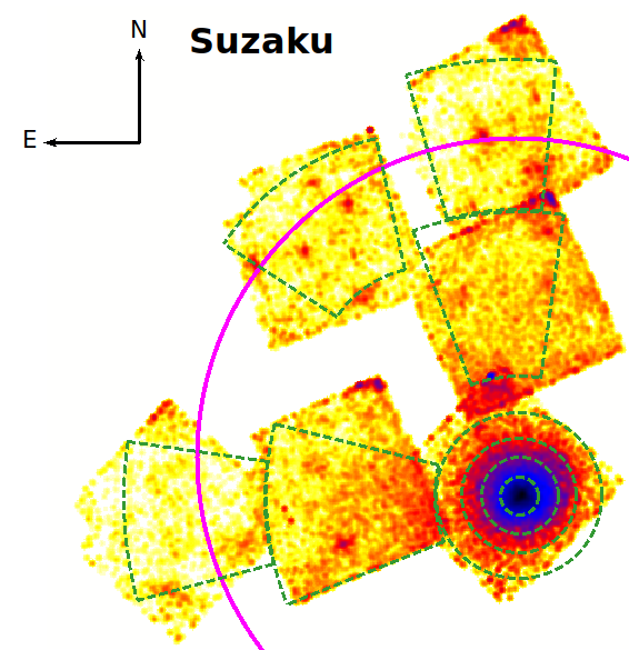
Figure 1: Left: Suzaku mosaic image of MWK4 in the 0.5-2 keV energy band with NXB subtracted and exposure corrected. Green annuli represent the regions used for spectra extraction. Magenta circle indicates R₂₀₀ = 33.2$\arcmin$ (884 kpc). Right: Chandra mosaic image of MKW4 center (ACIS-S3) and three outer regions (ACIS-I) in the 0.5-2.0 keV energy band. The image of MKW4 is smoothed with a Gaussian kernel and a number of radii of 30. Blue boxes represent the Suzaku FOV. Green elliptical regions are the resolved point sources. Magenta circle indicates R₂₀₀.

2.1 Suzaku

MKW4 has been mapped with three X-ray Imaging Spectrometer (XIS) instruments onboard Suzaku – two front-illuminated CCDs (XIS0, XIS3), and one back-illuminated CCD (XIS1). The observation logs are summarized in Table 1. All three XIS instruments were in the normal clocking mode without window and burst options during the observations.

Table 1: Observational log

Name	Obs Id	Instrument	Obs Date	Exposure time (ks)	RA (∘)	DEC (∘)	P.I.
Suzaku central	808066010	XIS0, XIS1, XIS3	2013 Dec 30	34.6	181.1346	1.9097	F. Gastaldello
Suzaku Offset 1	805081010	XIS0, XIS1, XIS3	2010 Nov 30	77.23	181.1270	2.2181	F. Gastaldello
Suzaku N2	808067010	XIS0, XIS1, XIS3	2010 Nov 30	97	181.1504	2.5206	Y. Su
Suzaku Offset 2	805082010	XIS0, XIS1, XIS3	2010 Nov 30	80	181.4270	1.8972	Y. Su
Suzaku E1	808065010	XIS0, XIS1, XIS3	2013 Dec 29	100	181.7142	1.8506	F. Gastaldello
Suzaku NE	809062010	XIS0, XIS1, XIS3	2013 Dec 29	87.5	181.4583	2.3361	Y. Su
Chandra central	3234	ACIS-S	2002 Nov 24	30	181.1283	1.9286	Y. Fukazawa
Chandra N	20593	ACIS-I	2019 Feb 25	14	181.1369	2.5209	Y. Su
Chandra E	20592	ACIS-I	2018 Nov 17	15	181.7146	1.8715	Y. Su
Chandra NE	20591	ACIS-I	2019 Mar 08	14	181.4548	2.3585	Y. Su

2.1.1 Data reduction

The Suzaku data was reduced using HEAsoft 6.25, CIAO 4.11, and the XIS calibration database (CALDB) version 20181010. We followed a standard data reduction thread to process all the event files. The 5$\times$5 mode event files were converted to the 3$\times$3 mode event files and combined with the other 3$\times$3 mode event files. The resulting event files were filtered for calibration source regions and bad pixels with cleansis. We selected events with GRADE 0, 2, 3, 4, and 6. Light curves were filtered for flares using the lc$\_$clean task of CIAO 4.11. The resolved point sources were identified visually. We did not exclude those sources while extracting spectra, because exclusion would result in a very low photon count available for the spectral analysis. We instead took the advantage of Chandra observations to estimate their position, flux and incorporated them in the background fit (discussed in Section 2.1.2).

We extracted spectra from four concentric annuli, $0\arcmin-2\arcmin$, $2\arcmin-4\arcmin$, $4\arcmin-6\arcmin$, and $6\arcmin-8.6\arcmin$ for the central pointing. We extracted spectra from two partial annuli $12.4\arcmin-29\arcmin$, $29\arcmin-48.3\arcmin$ for the pointings in the north direction and from $8.6\arcmin-26\arcmin$, $26\arcmin-45\arcmin$ for the pointings in the east direction. For the north-east direction, we extracted spectra from a partial annulus of $27\arcmin-42\arcmin$. All annuli had widths ranging from 8 kpc at the central region to 223 kpc at the outermost bin. We generated redistribution matrix files (RMF) for all regions and detectors using FTOOL xisrmfgen and instrumental background files (NXB) using FTOOL xisnxbgen. The ancillary response files (ARF) were generated using xissimarfgen by providing an appropriate $\beta$-image derived from the Chandra surface brightness profile of MKW4 at the central region. Another ARF was produced to model the X-ray background by considering uniform sky emission in a circular region of 20$\arcmin$ radius. An exposure corrected and NXB subtracted mosaic image of MKW4 in the 0.5-2 keV energy band is shown in Figure 1. We obtained Suzaku surface brightness profiles of MKW4 in three different directions, as shown in Figure 2. We fitted the profiles with a single $\beta$-model (Arnaud, 2009):

$${\rm S(r)}={\rm S_{0}}\left[1+\left(\frac{\rm r}{\rm r_{c}}\right)^{2}\right]^{-3\beta+1/2},$$ (2)

which yielded the best-fit ($\beta$, r${}_{\textrm{c}}$) = (0.515 $\pm$ 0.001, 30 $\pm$ 2.5 kpc).

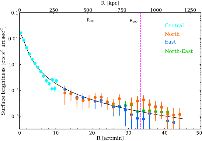
Figure 2: Surface brightness profiles of MKW4 derived from the Suzaku XIS image in the 0.5 - 2.0 keV energy band in three different directions. The profiles have been corrected for exposure, instrumental background (NXB), and the point sources detected with Chandra. Black solid line is the best-fit $\beta$-profile.

2.1.2 Spectral analysis

Spectral analysis was performed using XSPEC--12.10.1 and C-statistics. Each spectrum was rebinned to guarantee 20 photons per bin to aid the convergence and the computational speed. Spectra extracted from the XIS0, XIS1, and XIS3 were simultaneously fitted. The spectral fitting was restricted to the 0.4 - 7.0 keV energy band for XIS1, and to the 0.6 - 7.0 keV energy band for XIS0 and XIS3 (e.g., Mitsuda et al., 2007). We fitted each spectrum with an ICM emission model plus a multi-component X-ray background model. The ICM emission model contains a thermal apec component associated with a photoelectric absorption (phabs) component - phabs $\times$ apec, as shown in Figure 3. The temperature, abundance, and normalization of the apec component were allowed to vary independently for regions at the group center and at the intermediate radii. For those three regions at R₂₀₀, we find it necessary to fix their abundances at 0.2 $Z_{\odot}$. Similar metallicity was observed at R₂₀₀ for the RX J1159+5531 group (Su et al., 2015). We discuss the systematic uncertainties caused by this choice of abundance in Section 4.

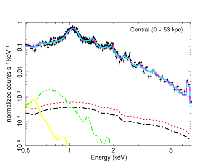
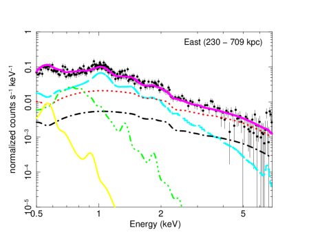
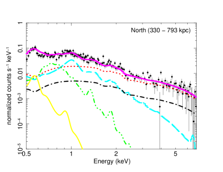
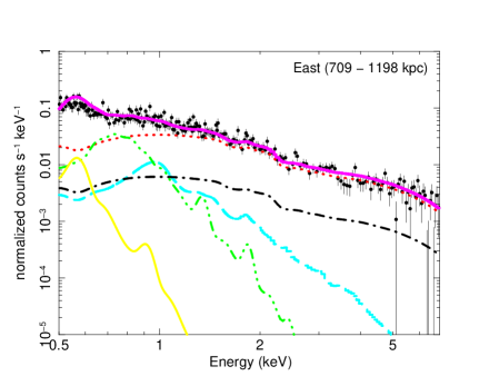
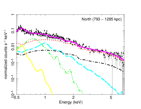
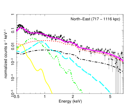
Figure 3: Suzaku XIS 1 spectra of MKW4 for representative regions of central and two outer bins in north and east directions. Black dots are the data points. Cyan, red, black, green, and yellow lines are the best-fit ICM emission, resolved CXB, unresolved CXB, MW, and LHB components, respectively. Magenta line is the model of the best-fit ICM emission and X-ray background components together.

To model the X-ray background, we adopted phabs$\times$(pow${}_{\textrm{resolved\ CXB}}$ + pow${}_{\textrm{unresolved\ CXB}}$ + apec${}_{\textrm{MW}}$) + apec${}_{\textrm{LHB}}$, where pow${}_{\textrm{resolved\ CXB}}$ and pow${}_{\textrm{unresolved\ CXB}}$ are the power-law components to model the resolved CXB and unresolved CXB, respectively. The thermal apec${}_{\textrm{MW}}$ and apec${}_{\textrm{LHB}}$ represent two foreground components to account for emissions from the Milky Way (MW) and Local Hot Bubble (LHB), respectively. We made use of the Chandra observations that cover the Suzaku pointings of the outskirts of MKW4 to mitigate much of the CXB contribution. We detected a total of 78 point sources with Chandra (see Figure 1). Point sources that fall onto the ACIS-S1, S2, and S4 chips are not included in our analysis. The faintest point source was detected at a flux of $8.1\times 10^{-15}$ erg cm^-2 s^-1. We converted the count rates of resolved point sources to the fluxes assuming a power-law model with a photon index of 1.41 (De Luca & Molendi, 2004). We produced mock Suzaku observations for the resolved point sources using xissim, based on their positions and fluxes determined with Chandra. An exposure time of 100 ks was set to ensure good photon statistics. We extracted spectra from the mock Suzaku observations using the same extraction regions used for the actual Suzaku observations. Figure 4 (left) compares the surface brightnesses of the actual point sources resolved by Chandra and that of the simulated Suzaku observations, which are in good agreement with each other. We fitted the mock spectra with an absorbed power-law model (phabs $\times$ pow) with a photon index of 1.41. The resulting best-fit normalizations were used as the normalizations of the resolved component (pow${}_{\textrm{resolved\ CXB}}$) in the background model and kept frozen. Figure 4 (right) compares the spectral temperature profiles (discussed in Section 3) obtained with Suzaku observations alone and with joint Suzaku and Chandra observations of MKW4 in the north-east direction. The significant improvement of uncertainties demonstrates that the addition of Chandra observations can help to constrain the CXB and increase the accuracy of the measurement of ICM properties at the outskirts (e.g., Miller et al., 2012). For the regions with no Chandra coverages (two regions of intermediate radii in north and east directions), we let the normalizations of pow${}_{\textrm{resolved\ CXB}}$ component to vary independently.

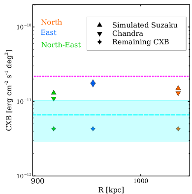
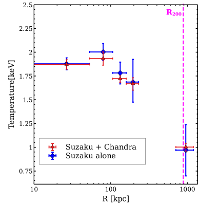
Figure 4: Left: Triangle down: surface brightness of point sources resolved by Chandra. Triangle up: surface brightness of point sources obtained from mock Suzaku sky. Magenta dotted: total surface brightness limit of resolved+unresolved point sources taken from Moretti et al. (2009). Cyan dashed: expected surface brightness limit of unresolved point sources with 1$\sigma$ error (shaded) calculated using Equations 3 and 4. Star: estimated surface brightness of unresolved point sources from Suzaku fitting. Right: Blue: spectroscopic temperature profile of MKW4 in the north-east direction obtained from spectral fitting of the Suzaku data only. Red: same profile obtained from the joint fitting of Suzaku and Chandra data. Magenta dashed line indicates R₂₀₀ of MKW4.

The normalizations of pow${}_{\textrm{unresolved\ CXB}}$ component were allowed to vary collectively for different regions, assuming little fluctuations in the surface brightness of the remaining unresolved point sources. We obtained a best-fit normalization of 4.2 $\times$ 10^-12 erg cm^-2 s^-1 deg^-2 for the unresolved point sources in the 2.0 - 10.0 keV energy band, as shown in Figure 4. The normalization of unresolved CXB can be estimated as (Moretti et al., 2009) -

$$\textrm{F}_{\textrm{CXB}}=2.18\pm 0.13\times 10^{-11}-\int_{\textrm{s}_{\textrm{min}}}^{\textrm{s}_{\textrm{max}}}{\left(\frac{\textrm{dN}}{\textrm{dS}}\right)\times\textrm{SdS}},$$ (3)

in units of erg cm^-2 s^-1 deg^-2, assuming a total CXB surface brightness of $2.18\pm 0.13\times 10^{-11}$ erg cm^-2 s^-1 deg^-2 in the 2.0 - 10.0 keV energy band. We adopted an analytical form of the integral source flux distribution from Moretti et al. (2003) -

$$\textrm{N}(>\textrm{S})=\textrm{N}_{\textrm{S(H)}}\left[\frac{(2\times 10^{-15})^{\alpha_{1,\textrm{S(H)}}}}{\textrm{S}^{\alpha_{1,\textrm{S(H)}}}+\textrm{S}_{\textrm{0,H}}^{\alpha_{1,\textrm{S(H)}}-\alpha_{2,\textrm{S(H)}}}\textrm{S}^{\alpha_{2,\textrm{S(H)}}}}\right],$$ (4)

where $\alpha_{1,\textrm{S(H)}}=1.57^{+0.10}_{-0.08}$, $\alpha_{2,\textrm{S(H)}}=0.44^{+0.12}_{-0.13}$, $\textrm{S}_{\textrm{{0,H}}}=4.5^{+3.7}_{1.7}\times 10^{-15}$ erg cm^-2 s^-1, and $\textrm{N}_{\textrm{S(H)}}=5300^{+2850}_{-1400}$ are the best-fit parameters with a 68% confidence level. We estimated the flux limit for unresolved point sources to be $6.61\pm 3.68\times 10^{-12}$ erg cm^-2 s^-1 deg^-2. This flux is consistent with the flux obtained from spectral fitting.

To constrain the temperature and surface brightness of Local Hot Bubble (apec${}_{\textrm{LHB}}$) and Milky Way (apec${}_{\textrm{MW}}$) foregrounds, we used the ROSAT All-Sky Survey (RASS) data in an annulus region of 0.9^∘ - 1.2^∘ from the group center where no group emission was expected. We extracted spectra using the HEASARC X-ray background tool. The RASS spectrum was fitted simultaneously with the Suzaku data. The background fitting results are shown in Figure 3 and listed in Table 2.

Table 2: X-ray background components of outer regions${}^{\textrm{a}}$

Name	CXB${}^{\textrm{b}}$	LHB${}^{\textrm{c}}$	MW${}^{\textrm{d}}$
Suzaku East	11.25${}^{+0.12}_{-0.13}$	13.9${}^{+1.1}_{-1.3}$	6.21${}^{+0.32}_{-0.35}$
Suzaku North	9.51${}^{+0.12}_{-0.12}$	$-$	$-$
Suzaku North-East	8.63${}^{+0.12}_{-0.12}$	$-$	$-$

${}^{\textrm{a}}$ Results for the normalizations of various components (non-instrumental) of X-ray background for a circular region with 20′ radii. The LHB and MW components for Suzaku North and Suzaku North-East directions are linked to the Suzaku East.
${}^{\textrm{b}}$ Normalization of power-law component ($\Gamma$=1.41) for resolved + unresolved cosmic X-ray background in the units of 10^-4 photons s^-1 cm^-2 keV^-1 at 1 keV.
${}^{\textrm{c}}$ Normalization of the unabsorbed apec thermal component (kT = 0.08 keV, abun= 1Z_⊙) integrated over line of sight, $1/4\pi[\textrm{D}_{\textrm{A}}(1+\textrm{z})]^{2}\int{\textrm{n}_{\textrm{e}}\textrm{n}_{\textrm{H}}\ \textrm{dV}}$ in the units of 10^-18 cm^-5.
${}^{\textrm{d}}$ Normalization of the absorbed apec thermal component (kT = 0.2 keV, abun= 1Z_⊙) integrated over line of sight, $1/4\pi[\textrm{D}_{\textrm{A}}(1+\textrm{z})]^{2}\int{\textrm{n}_{\textrm{e}}\textrm{n}_{\textrm{H}}\ \textrm{dV}}$ in the units of 10^-18 cm^-5.

2.2 Chandra

MKW4 was observed using Chandra with one ACIS-S pointing at the group center and three ACIS-I pointings overlapping with the outer regions observed with Suzaku . The observation logs are listed in Table 1.

2.2.1 Data reduction

The Chandra data reduction was performed using HEAsoft 6.25, CIAO-4.11, and a Chandra calibration database (CALDB 4.8.3). We followed a standard data reduction thread . All data were reprocessed from the level 1 events using chandra$\_$repro, which applied the latest gain, charge transfer inefficiency correction, and filtering from bad grades. The light curves were filtered using lc$\_$clean script to remove periods affected by flares. The resulting filtered exposure times are listed in Table 1. Point sources were identified with wavdetect using a range of wavelet radii between 1 and 16 pixels to maximize the number of detected point sources. The detection threshold was set to $10^{-6}$, which guaranteed detection of $\mathrel{\hbox{\hbox to0.0pt{\hbox{\lower 4.0pt\hbox{$\sim$}}\hss}\hbox{$<$}}}$ 1 spurious source per CCD. Detected point sources were confirmed visually. Figure 1 shows the adaptively smoothed ACIS-S3 image of MKW4 in the 0.5 - 2.0 keV energy band.

We extracted spectra from 6 adjoining, concentric annuli centered at the X-ray centroid in the Chandra ACIS-S3 chip. The widths of the annular regions were chosen to contain approximately the same number of background-subtracted counts of 2000 for better spectral analysis. Count-weighted spectral response matrices (ARFs and RMFs) were generated using mkwarf and mkacisrmf tasks for each annulus. The blanksky background was produced by the blanksky tool for background subtraction. The blanksky background was tailored based on the count rate in the 9.5 - 12.0 keV energy band relative to the observation.

2.2.2 Spectral analysis

All spectra were fitted simultaneously to model the ICM properties of different regions. We modeled the ICM emission with a single thermal apec model associated with a photoelectric absorption model- phabs $\times$ apec. Photoionization cross-sections were taken from Balucinska-Church & McCammon (1992). We obtained the galactic hydrogen column density, N${}_{\textrm{H}}$ = 1.72 $\times 10^{20}$ cm^-2 at the direction of MKW4, using HEASARC N${}_{\textrm{H}}$ tool . All ICM emission components were allowed to vary independently.

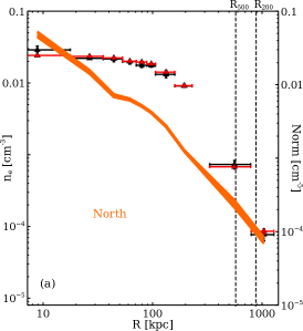
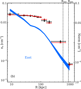
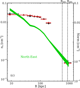
Figure 5: Deprojected density profiles of MKW4 in north (orange), east (blue), and north-east (green) directions. Shaded regions indicate 1$\sigma$ uncertainties. Red triangles: the best-fit normalizations for the apec thermal component obtained from spectral analysis. Black triangles: the normalizations of the apec thermal component calculated from the resulting 3D density profile.

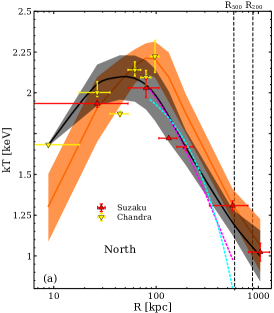
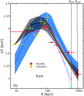
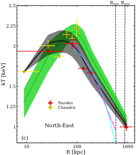
Figure 6: Deprojected temperature profiles of MKW4 in north (orange), east (blue), and north-east (green) directions. The 2D temperature profiles of MKW4, estimated using Equation 6, are indicated in black. Shaded regions indicate 1$\sigma$ uncertainties. Temperatures obtained from the apec thermal component by fitting the spectra extracted from the Chandra and Suzaku data are shown in yellow and red respectively. Magenta and cyan dashed lines show the average temperature profiles derived for groups in Loken et al. (2002) and Sun et al. (2009) respectively.

3 Results

3.1 Density and temperature profile

We derive the deprojected (3D) gas density and temperature profiles of MKW4 assuming analytical prescriptions for 3D gas density and temperature. We follow the analytical expressions described in Vikhlinin et al. (2006). The normalization of the apec thermal component relates to the ICM density as: norm = $\int{\textrm{n}_{\textrm{e}}\textrm{n}_{\textrm{p}}\ \textrm{dl}}$, where the density profile of electrons ($\textrm{n}_{\textrm{e}}$) and protons ($\textrm{n}_{\textrm{p}}$) can analytically be described as:

$$\begin{split}{\textrm{n}_{\textrm{e}}\textrm{n}_{\textrm{p}}{\rm(r)}}&{=\frac{\textrm{n}_{\textrm{01}}^{2}}{\left(1+\textrm{r}^{2}/\textrm{r}_{\textrm{c1}}^{2}\right)^{3\ \beta_{1}}}+\frac{\textrm{n}_{\textrm{02}}^{2}}{\left(1+\textrm{r}^{2}/\textrm{r}_{\textrm{c2}}^{2}\right)^{3\ \beta_{2}}}.}\end{split}$$ (5)

We obtain the 3D density profile of MKW4 by projecting the 3D analytic model given in Equation 5 along the line of sight and fit it to the measured 2D normalizations of thermal apec component obtained from the spectral analysis, assuming n_e = 1.2n_p and a fixed $\gamma$ = 3. The uncertainties are calculated using Monte Carlo simulations with 1000 to 2000 realizations.

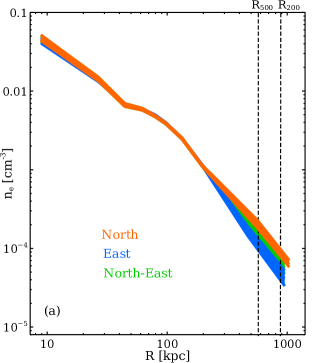
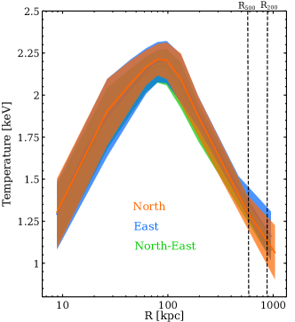
Figure 7: 3D density (left) and temperature (right) profiles of MKW4 in three different directions.

The resulting 3D density profiles are shown in Figure 5. A comparison between the normalizations obtained from spectral analysis and the normalizations obtained from the Equation 5 are also shown in Figure 5. Figure 7 compares the 3D density profiles of MKW4 in three different directions.

We derive the 3D temperature profile by fitting the spectral temperature (2D spectroscopic temperature, T${}_{\textrm{2D}}$) obtained from thermal apec component with the following analytic function (Vikhlinin et al., 2006):

$$\textrm{T}_{\textrm{2D}}=\frac{\int{\textrm{n}_{\textrm{e}}^{2}\ \textrm{T}_{\textrm{3D}}^{\frac{1}{4}}\ \textrm{dV}}}{\int{\textrm{n}_{\textrm{e}}^{2}\ \textrm{T}_{\textrm{3D}}^{-\frac{3}{4}}\ \textrm{dV}}},$$ (6)

where

$$\begin{split}\textrm{T}_{\textrm{3D}}(\textrm{r})&=\textrm{T}_{0}\frac{\left(\textrm{x}+\textrm{T}_{\textrm{min}}/\textrm{T}_{0}\right)}{\left(\textrm{x}+1\right)}\ \times\ \frac{\left(\textrm{r}/\textrm{r}_{\textrm{t}}\right)^{-\textrm{a}}}{\left(1+\textrm{r}^{\textrm{b}}/\textrm{r}_{\textrm{t}}^{\textrm{b}}\right)^{\textrm{c}/\textrm{b}}},\\ &\textrm{and}\ \ \textrm{x}=\left(\frac{\textrm{r}}{\textrm{r}_{\textrm{cool}}}\right)^{\textrm{a}_{\textrm{cool}}}.\end{split}$$ (7)

Figure 6 represents the projected (T${}_{\textrm{2D}}$) and deprojected (T${}_{\textrm{3D}}$) temperature profiles of MKW4 from its center out to the virial radii in north, east, and north-east directions.

The uncertainties in temperatures are also calculated using Monte Carlo simulations. The deprojected temperature profiles of MKW4 decline from 2.20 keV at 0.1R₂₀₀ to 1.14 keV at R₂₀₀. A similar temperature drop was found in other groups (e.g., Su et al., 2015). The projected temperatures measured with Suzaku and Chandra are consistent for the overlapping regions. Figure 7 compares the 3D temperature profiles of MKW4 in three different directions.

Our temperature profile agrees well with the Chandra temperature profiles of MKW4 out to R₂₅₀₀, as given by Vikhlinin et al. (2006) (V06) and Sun et al. (2009) (S09) as well as the measurement obtained with XMM-Newton by Gastaldello et al. (2007) (G07) out to $\sim$ 0.6R₅₀₀. We measure a gas temperature at R₅₀₀ between those of V06 and S09 and consistent with the Suzaku measurement using the two intermediate pointings (Sasaki et al., 2014). We compare the projected temperature profiles of MKW4 to the empirical profiles derived for groups by Sun et al. (2009):

$$\frac{\textrm{T}}{\textrm{T}_{\textrm{2500}}}=(1.22\ \pm\ 0.02)-(0.79\ \pm\ 0.04)\frac{\textrm{R}}{\textrm{R}_{500}}\ ,$$ (8)

and by Loken et al. (2002):

$$\frac{\textrm{T}}{\textrm{T}_{\textrm{2500}}}=(1.37\ \pm\ 0.03)-\left(1+\frac{\textrm{R}}{\textrm{R}_{500}}\right)^{-(1.34\ \pm\ 0.21)}\ ,$$ (9)

as shown in Figure 6. Both profiles show good agreement with the projected temperature profile of MKW4 out to $\sim$ R₂₅₀₀. Their values at R₅₀₀ exceed what is measured for MKW4 by 30% and 60%, respectively. These empirical profiles are determined with a large number of galaxy groups with a sizable scatter. Many of them do not have their temperatures actually measured out to R₅₀₀.

3.2 Entropy and pressure profile

We derive the 3D entropy and pressure profiles of MKW4 from 3D density and temperature profiles, as shown in Figures 8 and 9.

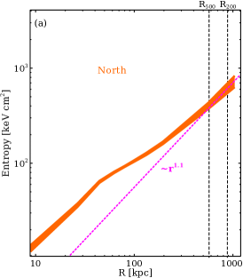
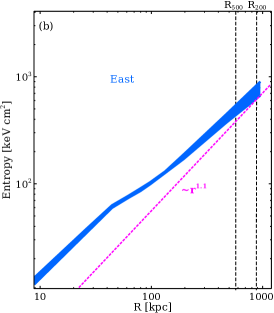
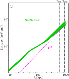
Figure 8: 3D entropy profiles of MKW4 in north (orange), east (blue), and north-east (green) directions. Shaded regions indicate 1$\sigma$ uncertainties. Magenta dashed line represents the entropy profile derived from gravity only cosmological simulation (Voit et al., 2005) using Equation 10.

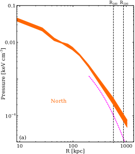
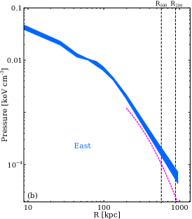
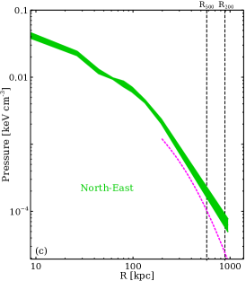
Figure 9: 3D pressure profiles of MKW4 in north (orange), east (blue), and north-east (green) directions. Shaded regions indicate 1$\sigma$ uncertainties. Magenta dashed line represents the semi-analytical universal pressure profile (Arnaud et al., 2010), derived using Equation 13.

We compare our entropy profiles with a baseline profile derived from purely gravitational structure formation (Voit et al., 2005) and assuming a hydrostatic equilibrium-

$$\textrm{K}_{\textrm{gra}}(\textrm{R})=1.32\ \textrm{K}_{200}\ \left(\frac{\textrm{R}}{\textrm{R}_{200}}\right)^{1.1},$$ (10)

and the normalization K₂₀₀ is defined as-

$$\begin{split}\textrm{K}_{200}&=362\frac{\textrm{G\ M}_{200}\ \mu\ \textrm{m}_{\textrm{p}}}{2\textrm{R}_{200}}\left(\frac{1}{\textrm{keV}}\right)\textrm{E}(\textrm{z})^{-4/3}\\ &\times\left(\frac{\Omega_{\textrm{m}}}{0.3}\right)^{-4/3}\textrm{keV cm}^{-2},\end{split}$$ (11)

$$\textrm{where,}\ \textrm{E}(\textrm{z})=\sqrt{\Omega_{\textrm{m}}\left(1+\textrm{z}\right)^{3}+\Omega_{\Lambda}}.$$ (12)

The m${}_{\textrm{p}}$ is proton mass and $\mu$ $\sim$ 0.6 is the mean molecular weight. The 3D entropy profiles of MKW4 increase monotonically with radius in three directions, as seen in Figure 8. We observe apparent entropy excesses towards the central region (up to $\sim$ 0.5R₂₀₀) of MKW4 relative to the baseline profile. At larger radii, the entropy profiles of MKW4 are consistent with the baseline profile, i.e., its slope attains a value of $\sim$ 1.1 between R₅₀₀ and R₂₀₀ in all observed directions.

The 3D pressure profiles of MKW4 are shown in Figure 9. We compare the measured pressure profiles to a semi-analytical universal pressure profile (Arnaud et al., 2010) defined as -

$$\begin{split}\textrm{P}(\textrm{r})&=\textrm{P}_{500}\left[\frac{\textrm{M}_{500}}{3\times 10^{14}\textrm{h}_{70}^{-1}\textrm{M}_{\odot}}\right]^{\alpha_{\textrm{p}}+\alpha^{{}^{\prime}}_{\textrm{p}}(\textrm{x})}\\ &\ \ \ \ \ \ \ \ \ \ \ \ \ \ \ \ \ \ \times\frac{\textrm{P}_{0}}{\left(\textrm{c}_{500}x\right)^{\gamma}\left[1+\left(\textrm{c}_{500}x\right)^{\alpha}\right]^{\frac{\left(\beta-\alpha\right)}{\alpha}}}\end{split}$$ (13)

where x = $\frac{\textrm{R}}{\textrm{R}_{500}}$, $\alpha^{{}^{\prime}}_{\textrm{p}}(\textrm{x})$ = $0.10-(\alpha_{\textrm{p}}+0.10)\frac{(\textrm{x}/0.5)^{3}}{[1+(\textrm{x}/0.5)^{3}]}$. The P₅₀₀ is the pressure at R₅₀₀ and M₅₀₀ (see Table LABEL:tab:prop) is the total hydrostatic mass within R₅₀₀. We adopt

$$[\textrm{P}_{0},\ \textrm{c}_{500},\ \alpha,\ \beta,\ \gamma,\ \alpha_{\textrm{p}}]=$$

$$[8.403\textrm{h}_{70}^{-3/2},\ 1.177,\ 0.3081,\ 1.0510,\ 5.4905,\ 0.12\pm 0.10]$$

from Arnaud et al. (2010). Sun et al. (2011) adopted similar parameters and found that the Arnaud et al. (2010) pressure profile is also representative for galaxy groups. The 3D pressure profiles of MKW4 in all directions from 0.35R₅₀₀ out to $\sim$ 0.65R₅₀₀ show good agreement with this universal pressure profile but exceed it by more than 50% at R₅₀₀.

3.3 Mass and gas fraction

We derive the X-ray hydrostatic mass of MKW4 and its gas mass within a specific radius (R) from the group center, incorporating the above 3D density and temperature profiles in the following equations-

$$\textrm{M}_{\textrm{tot}}(<\textrm{R})=-\frac{\textrm{kT}_{\textrm{3D}}\textrm{R}}{\textrm{G}\mu\textrm{m}_{\textrm{p}}}\left(\frac{\textrm{d\ ln}\rho_{\textrm{gas}}}{\textrm{d\ ln}\textrm{R}}+\frac{\textrm{d\ ln}\textrm{T}_{\textrm{3D}}}{\textrm{d\ ln}\textrm{R}}\right)$$ (14)

$$\textrm{M}_{\textrm{gas}}(<\textrm{R})=4\pi\ \int_{0}^{\textrm{R}}\ \rho_{\textrm{g}}(\textrm{r}^{\arcmin})\textrm{r}^{\arcmin 2}\textrm{dr}^{\arcmin},$$ (15)

where $\rho_{\textrm{gas}}$ = 1.92$\mu$m_Hn_e is the gas density, and m_H is the proton mass. The resulting hydrostatic mass profile of MKW4 is shown in Figure 10. We obtain $\textrm{M}_{\textrm{tot}}(<\textrm{R}_{500})$ $\approx$ 6.5 $\pm$ 1.0 $\times$ 10¹³ $\textrm{M}_{\odot}$ and $\textrm{M}_{\textrm{tot}}(<\textrm{R}_{200})$ $\approx$ 9.7 $\pm$ 1.5 $\times$ 10¹³ $\textrm{M}_{\odot}$.

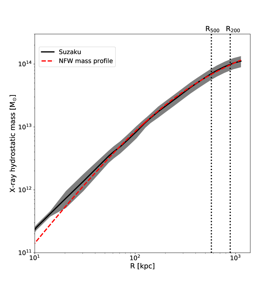
Figure 10: The X-ray hydrostatic mass profile (M${}_{\textrm{total}}$) of MKW4 derived using Equation 14. Red dashed line shows best-fit NFW mass profile obtained by integrating Equation 16. Shaded region indicates 1$\sigma$ error.

Our measured hydrostatic mass within R₅₀₀ is between that given by Vikhlinin et al. (2006) ( 7.7 $\pm$ 1.0 $\times$ 10¹³ $\textrm{M}_{\odot}$) and those of Gastaldello et al. (2007) (4.3 $\pm$ 0.2 $\times$ 10¹³ $\textrm{M}_{\odot}$) and Sun et al. (2009) (4.8 $\pm$ 0.7 $\times$ 10¹³ $\textrm{M}_{\odot}$).

We fit our hydrostatic mass profile to the NFW mass density profile (Navarro et al., 1997):

$$\rho({\rm r})=\frac{\rho_{\rm s}}{({\rm r}/{\rm r}_{\rm s})(1+{\rm r}/{\rm r}_{\rm s})^{2}},$$ (16)

as shown in Figure 10. We obtain a best-fit r_s of 186 $\pm$ 23 kpc, which gives the central mass concentrations of c₅₀₀ = 3.09${}^{+0.52}_{-0.39}$ at R₅₀₀ and c₂₀₀ = 4.75${}^{+0.80}_{-0.60}$ at R₂₀₀. We also obtain the sparsity, the ratio of masses at two overdensities (Corasaniti et al., 2018), S_200,500 = 1.49 $\pm$ 0.31. Our measurement of S_200,500 for MKW4 is closely align with the typical S_200,500 of 1.5 found for galaxy clusters in N-body simulation (Corasaniti et al., 2018).

Table 3: Properties of MKW4

T${}_{2500}^{\textrm{a}}$

T500

T200

R2500

R500

R200

M${}_{500}^{\textrm{b}}$

M200

f${}_{\textrm{gas, 2500}}^{\textrm{c}}$

f${}_{\textrm{gas, 500}}$

f${}_{\textrm{gas, 200}}$

c500

c200

(keV)

(keV)

(keV)

(kpc)

(kpc)

(kpc)

(1013 M⊙)

(1013 M⊙)

1.71${}^{+0.09}_{-0.08}$

1.36 $\pm$ 0.09

1.14${}^{+0.16}_{-0.13}$

274 $\pm$ 10

574 $\pm$ 20

884 $\pm$ 17

6.5 $\pm$ 1.0

9.7 $\pm$ 1.5

0.05 $\pm$ 0.01

0.07 $\pm$ 0.01

0.090 $\pm$ 0.011

3.09${}^{+0.52}_{-0.39}$

4.75${}^{+0.80}_{-0.60}$

We obtain its enclosed gas mass and estimate the gas mass fraction f${}_{\textrm{gas}}$ = $\frac{\textrm{M}_{\textrm{gas}}}{\textrm{M}_{\textrm{tot}}}$ for each direction, as shown in Figure 11. At $\sim$ R₅₀₀, the measured gas mass fraction of MKW4 is below 10% in all directions, similar to the other galaxy groups (e.g., Vikhlinin et al., 2006; Sun et al., 2009; Humphrey et al., 2012; Thölken et al., 2016). At a radii larger than R₅₀₀, f${}_{\textrm{gas}}$ grows slowly and attains a value of 0.092 $\pm$ 0.009 in the north, 0.087 $\pm$ 0.012 in the east, and 0.090 $\pm$ 0.011 in the north-east at R₂₀₀. These gas mass fractions are surprisingly low compared to the cosmic baryon fraction of 0.15 (Planck Collaboration et al., 2014) and 0.17 (Komatsu et al., 2011). A brief comparison of the mass and f_gas of MKW4 between our work and previous studies is listed in Table LABEL:tab:com.

Table 4: Comparison of our results with other works

Name	R500	M${}_{500}^{\ddagger}$	f${}_{\textrm{gas, 2500}}^{\dagger}$	f${}_{\textrm{gas, 500}}^{\dagger}$	c${}_{\textrm{500}}$
	(kpc)	$\times$ 1013 (M⊙)
This work	574 $\pm$ 20	6.5 $\pm$ 1.0	0.05 $\pm$ 0.01	0.07 $\pm$ 0.01	3.09${}^{+0.52}_{-0.39}$
S09$	538${}^{+24}_{-29}$	4.85${}^{+0.71}_{-0.68}$	0.047${}^{+0.002}_{-0.003}$	0.086 $\pm$ 0.009	3.93${}^{+1.16}_{-0.78}$
G07	527 $\pm$ 8	4.27 $\pm$ 0.18	$-$	$-$	6.4 $\pm$ 0.5
V06	634 $\pm$ 28	7.7 $\pm$ 1.0	0.045 $\pm$ 0.002	0.062 $\pm$ 0.006	2.54 $\pm$ 0.15

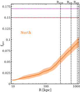
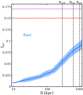
Figure 11: The gas mass fraction of MKW4 in north (orange), east (blue), and north-east (green) directions. Red dashed line: cosmic baryon fraction estimated by Planck (Planck Collaboration et al., 2014). Magenta dashed line: cosmic baryon fraction estimated by WMAP (Komatsu et al., 2011).

4 Systematic uncertainties

We investigate changes of the best-fit gas density, temperature, entropy, pressure, and enclosed gas mass fraction at R₂₀₀ introduced by a variety of systematic effects. Below we focus on the systematic uncertainties related to the entropy. All other gas properties are listed in Table 5.

Table 5: Systematic error of gas properties at R${}_{\textrm{200}}$

	Test	Temperature	Density	Entropy	Pressure	f${}_{\textrm{gas}}$
		keV	10-5 cm-3	keV cm2	10-5 keV cm-3
	Best fit	1.13 $\pm$ 0.14	8.85 $\pm$ 1.5	630 $\pm$ 82	9.2 $\pm$ 2.8	0.092 $\pm$ 0.009
North	$\Delta$CXB	+0.06, $-$0.04	+0.08, $-$0.46	$-$4, +176	+0.17, $-$0.36	$\pm$0.004
	$\Delta$CXB-$\Gamma$	+0.14, $-$0.04	$-$0.24, $-$0.13	$-$26, +116	$-$0.8, +0.003	$\pm$0.001
	$\Delta$abun	+0.06, $-$0.04	+0.22, $-$0.46	$-$22, +177	+0.03, $-$0.36	+0.0007, $-$0.008
	$\Delta$N${}_{\textrm{H}}$	$-$0.04, +0.06	$-$0.22, $-$0.15	+31, +30	$-$0.09, +0.4	$-$0.002, +0.009
	$\Delta$distance	$\pm$0.03	$\pm$0.2	$\pm$66	$\pm$0.34	$\pm$0.008
	$\Delta$MW	+0.084, +0.024	+0.001, $-$0.19	$-$51, +72	+0.20, +0.16	+0.001, +0.001
	$\Delta$LHB	$\pm$0.09	$\pm$0.05	$\pm$165	$\pm$0.16	$\pm$0.01
	$\Delta$solar	+0.02, +0.14	$-$0.66, $-$0.23	+159, $-$28	$\pm$0.78	+0.01, +0.02
	Best fit	1.17 $\pm$ 0.15	5.6 $\pm$ 1.2	712 $\pm$ 100	6.55 $\pm$ 1.3	0.087 $\pm$ 0.012
East	$\Delta$CXB	+0.28, $-$0.1	+1.52, +0.84	+71, $-$141	+2.4, $-$0.03	+0.006, $-$0.001
	$\Delta$CXB-$\Gamma$	$-$0.2, +0.28	+1.06, +1.27	$-$249, +107	$-$0.27, +2.08	$-$0.006, +0.005
	$\Delta$abun	+0.28, $-$0.10	+0.85, +1.55	$-$68, +143	$-$0.02, +2.44	+0.005, $-$0.001
	$\Delta$N${}_{\textrm{H}}$	$-$0.01, +0.05	+0.12, +0.13	$-$63, $-$55	+0.13, +0.88	+0.003, +0.02
	$\Delta$distance	$\pm$0.02	$\pm$0.34	$\pm$39	$\pm$0.06	$\pm$0.002
	$\Delta$MW	$-$0.06, +0.16	+0.9, +0.43	$-$186, +167	+0.23, +0.49	-0.01, +0.03
	$\Delta$LHB	$\pm$0.01	$\pm$0.62	$\pm$82	$\pm$0.17	$\pm$ 0.001
	$\Delta$solar	+0.06, $-$0.1	+0.16, +1.27	+111, $-$191	$-$0.11, +0.36	$-$0.003, +0.008
	Best fit	1.12 $\pm$ 0.07	6.7 $\pm$ 1.8	682 $\pm$ 134	7.54 $\pm$ 1.7	0.090 $\pm$ 0.011
North-East	$\Delta$CXB	+0.09, $-$0.25	+1.2, $-$0.36	$-$5, +130	+1.4, $-$0.3	$-$0.01, $-$0.005
	$\Delta$CXB-$\Gamma$	+0.06, $-$0.25	$-$1.4, $-$1.27	+210, $-$44	$-$1.7, $-$2.8	+0.003, $-$0.004
	$\Delta$abun	$-$0.15, $-$0.07	$-$0.74, $-$1.8	$-$39, +213	$-$1.8, $-$2.6	$-$0.003, $-$0.004
	$\Delta$N${}_{\textrm{H}}$	$-$0.05, +0.06	$-$0.14, $-$0.13	$-$34, +40	$-$0.80, $-$0.70	$-$0.004, 0.007
	$\Delta$distance	$\pm$0.05	$\pm$1.4	$\pm$152	$\pm$2.1	$\pm$ 0.003
	$\Delta$MW	$-$0.15, +0.05	$-$0.67, $-$0.95	$-$61, +200	$-$0.93, $-$0.61	$-$0.004, $-$0.008
	$\Delta$LHB	$\pm$0.03	$\pm$0.78	$\pm$201	$\pm$0.57	$\pm$0.002
	$\Delta$solar	$-$0.07, $-$0.25	$-$2.0, $-$1.2	+235, $-$60	$-$2.8, +2.7	$\pm$0.004

We consider two different sources of systematic uncertainties associated with the CXB. First, we allow the best fit normalization of the CXB component in the background model to vary by 20% with a fixed power-law slope of $\Gamma$ = 1.41 (De Luca & Molendi, 2004), which leads to a maximum change in gas entropy by $\sim$ 18% at R₂₀₀ for the north, east, and north-east directions (see $\Delta$CXB in Table 5). Second, we fix the CXB power-law slope to $\Gamma$ = 1.3 and 1.5, respectively. Adopting $\Gamma$ = 1.3 has little effect on our results for the north direction, while the gas entropy varies by $\sim$ 30% for the other two directions. Adopting $\Gamma$ = 1.5, the gas entropy is increased by $\sim$ 14% for the north and east directions, while no significant changes are observed for the north-east direction.

We examine the impacts on gas properties due to variations in the MW and LHB foreground components by varying the normalization of each component by 10% (see $\Delta$MW and $\Delta$LHB in Table 5). We find that the variation in the MW component changes the gas entropy by 22% in the east and 27% in the north-east. The 10% variation in the LHB component changes the entropy by 20% in the north and 27% in the north-east.

We adopt the solar abundance table of Asplund et al. (2006) for the spectral analysis, as shown in Figure 3. Here, we experiment with two different solar abundance tables of Anders & Grevesse (1989) and Lodders (2003) to find their impacts on the measurement of gas properties. Results are listed in Table 5 under $\Delta$solar. Using the Anders & Grevesse (1989) solar abundance table, the gas entropy increases by 20% in the north, 13% in the east, and 32% in the north-east directions. In contrast, using the Lodders (2003) abundance table, the entropy does not change significantly in the north and north-east directions but decreases by 20% in the east.

In the spectral analysis, we find it necessary to fix the ICM metallicity at 0.2 $Z_{\odot}$ for regions at R₂₀₀. Here, we estimate the uncertainties in the measurements of gas properties associated with the possible variation of the ICM metallicity. We repeat the spectral analysis by fixing the metallicity at 0.1 $Z_{\odot}$ and 0.3 $Z_{\odot}$ (see $\Delta$abun in Table 5). Fixing the metal abundance at 0.1 $Z_{\odot}$ has little impact on gas properties at the outskirts of MKW4, while adopting a metalicity of 0.3 $Z_{\odot}$ increases the gas entropy by $\sim$ 20% in the north, 15% in the east, and 25% in the north-east directions.

5 Discussion

Combining the deep Suzaku observations with the Chandra ACIS-S and ACIS-I observations of MKW4, we measured its gas properties from the group center out to the virial radii in three directions. Its entropy profiles at larger radii are consistent with the self-similar value predicted by gravitational collapse alone (Voit et al., 2005). We estimated the enclosed gas mass fraction of MKW4 as a function of radial distance from the group center and obtained a surprisingly low value within R₂₀₀ compared to clusters. Below we discuss the implications of these results in detail.

5.1 Entropy profile

The entropy profile describes the thermal history of the ICM. Previous works on massive clusters (T${}_{\textrm{X}}>$3 keV) have measured entropy profiles that flatten between R₅₀₀ and R₂₀₀ and even tend to fall below the self-similar value predicted by gravitational collapse alone (e.g., Simionescu et al., 2011; Bonamente et al., 2013; Walker et al., 2012a). The explanations proposed for the unexpected entropy profiles include clumpy ICM and electron-ion non-equilibrium, either of which can be induced as galaxy clusters accrete cold gas from cosmic filaments. Using numerical simulations, Nagai & Lau (2011) predict that massive clusters with $\textrm{M}_{200}>10^{14}\textrm{M}_{\odot}\textrm{ h}^{-1}$ contain a significant fraction of clumpy gas at larger radii due to frequent merging events, which biases low the entropy by overestimating the gas density. We do not observe any flattening in the entropy profiles of MKW4 between R₅₀₀ and R₂₀₀. Our results suggest that the merger rate is comparably lower for MKW4 because of the shallow gravitational potential well, which makes the ICM less clumpy at its outskirts. This also supports the fact that clumping factors are smaller in the low mass clusters (M${}_{200}<10^{14}\textrm{M}_{\odot}\textrm{h}^{-1}$) and groups, as suggested by Su et al. (2015), Thölken et al. (2016), and Bulbul et al. (2016). The entropy profiles of MKW4 instead follow the baseline profile (Voit et al., 2005), indicating its gas dynamics at the outskirts may be mainly regulated by gravity.

Another explanation for entropy flattening is electron-ion thermal non-equilibrium. A shock wave resulting from any recent merger and accretion event at the outskirts tends to heat the heavy-ions faster than electrons, causing the ion temperature to exceed the electron temperature. This thermal non-equilibrium could bias low the gas entropy. Numerical simulations show that the discrepancy between electron and ion temperature is more severe in more massive and rapidly growing clusters (e.g., Avestruz et al., 2015; Walker et al., 2019). The well behaved entropy profiles of MKW4 suggest that it is a relatively undisturbed system and has experienced few recent mergers.

Despite the agreement between the entropy profiles of MKW4 and the baseline profile (Voit et al., 2005) at larger radii, we observe apparent entropy excess at the center of MKW4. Pratt et al. (2010) and Le Brun et al. (2014) advocate that the AGN feedback could elevate entropy profiles at the center of galaxy clusters by pushing a substantial fraction of baryons out of R₂₀₀. Pratt et al. (2010) also corrects the entropy profiles for the redistribution of hot gas due to AGN feedback, as follows-

$$\textrm{K}_{\textrm{corrected}}=\textrm{K}_{\textrm{measured}}\ \times\ \left(\frac{\textrm{f}_{\textrm{gas}}}{\textrm{f}_{\textrm{b}}}\right)^{2/3}.$$ (17)

We scale the measured entropy profile of MKW4 in north direction as Equation 17, adopting a cosmic baryon fraction of f${}_{\textrm{b}}$ = 0.15 from the Planck Collaboration et al. (2014), as shown in Figure 12. We find the scaled entropy profile follows closely with the baseline profile, even out to the virial radii, suggesting that the redistribution of the group gas due to the AGN feedback may have shaped its gas entropy (Mathews & Guo, 2011).

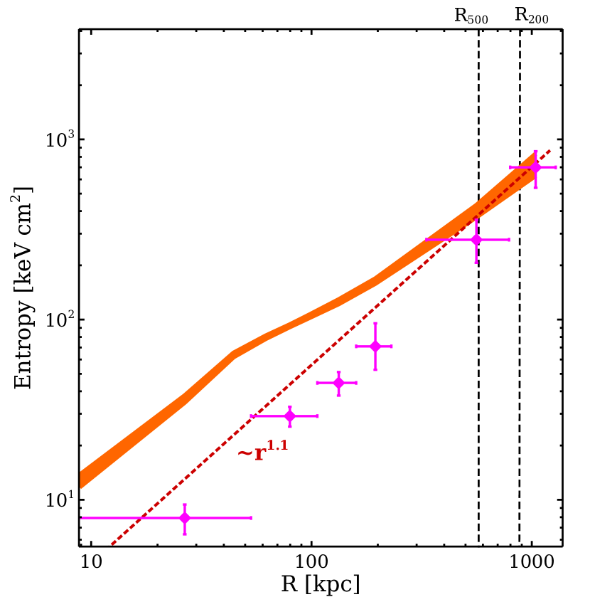
Figure 12: Orange: The entropy profile of MKW4 in north direction with 1$\sigma$ error. Red: The baseline entropy profile estimated using Equation 10. Magenta: The entropy profile scaled with f${}_{\textrm{gas}}$ as shown in Equation 17.

5.2 Gas mass fraction

The enclosed gas mass fraction (f${}_{\textrm{gas}}$) of MKW4 slowly rises from the group center and reaches $\sim$ 7% within R₅₀₀, consistent with the previous Chandra studies of MKW4 (Vikhlinin et al., 2006) and the f${}_{\textrm{gas}}$ of other groups (e.g., Humphrey et al., 2012; Su et al., 2013; Lovisari et al., 2015; Su et al., 2015; Thölken et al., 2016). We obtain a f${}_{\textrm{gas}}$ of $\sim$ 9% within R₂₀₀ for MKW4, which is remarkably small compared to the cosmic baryon fraction (f${}_{\textrm{b}}$) of 15%.

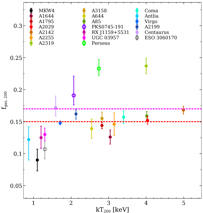
Figure 13: The f_gas is plotted with the cluster temperature at R₂₀₀. Open circles represent f_gas obtained using Suzaku only and filled circles represent f_gas obtained using XMM-Newton + Planck or Suzaku + Chandra. Color codes for different clusters are shown in the plot. The f_gas for A1644, A1795, A2029, A2142, A2255, A2319, A3158, A644, and A85 are taken from Eckert et al. (2019). We obtain f_gas of PKS0745-191 from Walker et al. (2012b), RX J1159+5531 from Su et al. (2015), UGC 03957 from Thölken et al. (2016), Coma from Mirakhor & Walker (2020a), Perseus from Simionescu et al. (2011), Antlia from Wong et al. (2016), Virgo from Simionescu et al. (2017), A2199 from Mirakhor & Walker (2020b), Centaurus from Walker et al. (2013), and ESO 3060170 from Su et al. (2013). Red and magenta dashed lines shows cosmic baryon fraction estimated using Planck (Planck Collaboration et al., 2014) and WMAP (Komatsu et al., 2011) respectively.

We estimate the stellar mass of MKW4 using Two Micron All-Sky Survey (2MASS) data in K${}_{\textrm{s}}$ band, assuming a stellar mass-to-light ratio of $\sim$ 1 (Bell et al., 2003). We find that the stellar mass contributes nearly 2% to the total hydrostatic mass, which leads to an enclosed baryon fraction (f${}_{\textrm{b}}$) of $\sim$ 11% within R₂₀₀ of MKW4, still significantly lower than the cosmic f${}_{\textrm{b}}$.

Similar discrepancies have been found in galaxies (e.g., Fukugita et al., 1998; Hoekstra et al., 2005; Dai et al., 2010), the so called “missing baryon problem”, which remains a grand challenge problem in understanding the galaxy evolution (e.g., Fukugita et al., 1998; Dai et al., 2010). In the case of MKW4, internal heating caused by AGN feedback may have pushed the hot gas towards larger radii or even expelled it from the system (e.g., Metzler & Evrard, 1994; Bower et al., 2008), which reduces the amount of hot gas, hence the baryon fraction. Alternatively, a significant amount of hot gas associated with the individual galaxies may have condensed and cooled out of the X-ray emitting ICM and reside in the Circumgalactic Medium (CGM) in the form of cold gas (e.g., Fielding et al., 2017) that is undetectable in X-ray and near-infrared (K${}_{\textrm{s}}$ band). Massive systems such as clusters of galaxies typically have a f${}_{\textrm{b}}$ consistent with the cosmic f${}_{\textrm{b}}$ at the virial radii (e.g., Walker et al., 2012a; Bonamente et al., 2013), while the f${}_{\textrm{b}}$ of galaxies is approximately 7% (Hoekstra et al., 2005) at their virial radii.

We note that MKW4, as a galaxy group, has a f${}_{\textrm{b}}$ within R₂₀₀ between those of galaxies and clusters. We compare our estimated f${}_{\textrm{gas}}$ at R₂₀₀ (f${}_{\textrm{gas, 200}}$) with those of other clusters and groups as a function of cluster temperature at R₂₀₀, as shown in Figure 13. The f_gas,200 of lower-mass clusters tend to stay below the cosmic baryon fraction. In contrast, the intermediate and higher-mass clusters have f_gas,200 consistent with the cosmic baryon fraction. Gravitational potential may have played a critical role in retaining hot baryons inside a galaxy cluster.

The measured f_gas,200 of PKS 0745, Perseus, and A2319 exceed the cosmic baryon fraction. The f_gas,200 of PKS 0745 and Perseus were measured with Suzaku alone, which may introduce positive bias in the gas mass measurement due to unresolved cool gas clumps at their outskirts. A2319 is a merging cluster, for which Ghirardini et al. (2018) report a substantial non-thermal pressure support at its outskirts, which may have biased the hydrostatic mass low. Our estimated f_gas,200 in MKW4 is consistent with other groups of similar masses, as seen in Figure 13. The low f_gas,200 found in MKW4 implies that its X-ray hydrostatic mass is unlikely to be underestimated at R₂₀₀.

5.3 Azimuthal Scatter

Azimuthal variations in the ICM properties may arise for different reasons, including unresolved substructures, mergers, and gas clumping (e.g., Miller et al., 2012; Su et al., 2015). We adopt the formula given by Vazza et al. (2011) to evaluate the azimuthal scatter of different gas properties at the outskirts of MKW4 and compare our results with the other clusters and groups-

$$\textrm{S}_{\textrm{c}}(\textrm{r})=\sqrt{\frac{1}{\textrm{N}}\sum_{\textrm{i}}\frac{\left[\textrm{y}_{\textrm{i}}(\textrm{r})-\textrm{Y}(\textrm{r})\right]^{2}}{\left[\textrm{Y}(\textrm{r})\right]^{2}}},$$ (18)

where y${}_{\textrm{i}}(\textrm{r})$ is the radial profile of a quantity for the i${}^{\textrm{th}}$-section, Y(r) is the azimuthal average of that quantity, and N is the total number of sections. We obtain azimuthal scatters of gas properties at R₂₀₀ of MKW4, as shown in Figure 14. We find S${}_{\textrm{c}}(\textrm{R}_{200})$ = 0.041 $\pm$ 0.012 in temperature, 0.191 $\pm$ 0.036 in density, 0.052 $\pm$ 0.019 in entropy, 0.149 $\pm$ 0.037 in pressure, and 0.020 $\pm$ 0.009 in the gas mass fraction.

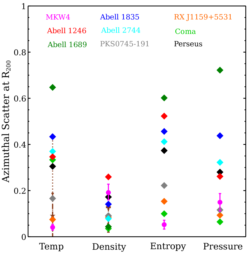
Figure 14: Azimuthal scatter of gas properties at R₂₀₀ of MKW4. We compare our results with azimuthal variations in other clusters, e.g., A1246: Sato et al. (2014); A1689: Kawaharada et al. (2010); A1835: Ichikawa et al. (2013); A2744: Ibaraki et al. (2014); PKS0745-191: George et al. (2009); RJX1159+5531: Su et al. (2015); Coma: Simionescu et al. (2013); Perseus: Urban et al. (2014b). Dashed brown line: the azimuthal variation in relaxed simulated clusters from Vazza et al. (2011). Dotted brown line: the azimuthal variation in perturbed simulated clusters from Vazza et al. (2011).

Numerical simulations show that the azimuthal variation in gas density and temperature rises to $\sim$ 10% at R₂₀₀ for relaxed clusters, while it increases to $\sim$ 50-80% for perturbed clusters (Vazza et al., 2011), as shown in Figure 14. The azimuthal scatters of the gas properties at the outskirts of MKW4 are consistent with the expectation for relaxed clusters. We also compare our results with a number of galaxy clusters observed with Suzaku out to R₂₀₀ with $N$ = 3 or more azimuthal coverages, as shown in Figure 14. The azimuthal variations in temperature and entropy of MKW4 are significantly smaller among those clusters. The similar ICM properties at R₂₀₀ in the north, east, and north-east directions confirm that MKW4 is a spherically symmetric relaxed system, and the hydrostatic equilibrium is likely to be a good approximation even out to its virial radii.

6 Summary

We have analysed joint Suzaku and Chandra observations of the galaxy group MKW4 and measured its ICM properties from its center out to the virial radius. We have derived the radial profiles of gas density, temperature, entropy, pressure, and gas mass fraction in three different directions. Our findings are summarized below.

• Using Chandra observations of MKW4, we have resolved much of the CXB at its center and three outskirt regions. We are able to model the contamination from point sources in Suzaku data and greatly reduce the uncertainties in the measurement of ICM properties.

• The 3D gas densities of MKW4 decline to $\sim$ 10^-5 cm^-3 at its outskirts and are consistent among the three directions. The 3D temperature profiles decline from 2.2 keV at 0.1R₂₀₀ to $\sim$ 1.14 keV at the virial radius. The temperature profiles of MKW4 in the three directions follow the universal profiles are derived by Loken et al. (2002) and Sun et al. (2009).

• The entropy profiles of MKW4 follow the baseline profile (Voit et al., 2005) beyond R₅₀₀ in the north, east, and north-east directions, which indicates that the gas dynamics at the group outskirts is mainly regulated by the gravitational collapse. Our results also show entropy excess towards the group center compared to the baseline profile, suggesting that the central AGN of MKW4 may have redistributed the hot gas.

• We estimated the total X-ray hydrostatic mass of MKW4, $\textrm{M}_{\textrm{tot}}(<\textrm{R}_{500})$ $\approx$ 6.5 $\pm$ 1.0 $\times$ 10¹³ $\textrm{M}_{\odot}$ and $\textrm{M}_{\textrm{tot}}(<\textrm{R}_{200})$ $\approx$ 9.7 $\pm$ 1.5 $\times$ 10¹³ $\textrm{M}_{\odot}$. Our measurement shows that its baryon fraction is only $\sim$ 11% at the virial radii, which is lower than the cosmic baryon fraction (Komatsu et al., 2011; Planck Collaboration et al., 2014). The lower baryon fraction implies that the central AGN feedback or galactic winds may have expelled much of its hot gas at its early epoch, or/and the hot gas associated with the individual galaxies may have condensed and cooled out of the X-ray emitting ICM and reside in the CGM in the form of cold gas.

• The azimuthal scatter in gas properties at the outskirts of MKW4 is small, suggesting that it is a remarkably relaxed system and the bulk of its ICM is likely to be in hydrostatic equilibrium.

Data Availability

The data underlying this article will be shared on reasonable request to the corresponding author.

References

- Akamatsu et al. (2011) Akamatsu H., Hoshino A., Ishisaki Y., Ohashi T., Sato K., Takei Y., Ota N., 2011, Publications of the Astronomical Society of Japan, 63, S1019
- Anders & Grevesse (1989) Anders E., Grevesse N., 1989, Geochimica et Cosmochimica Acta, 53, 197
- Arnaud (2009) Arnaud M., 2009, A&A, 500, 103
- Arnaud et al. (2010) Arnaud M., Pratt G. W., Piffaretti R., Böhringer H., Croston J. H., Pointecouteau E., 2010, A&A, 517, A92
- Asplund et al. (2006) Asplund M., Grevesse N., Sauval] A. J., 2006, Nuclear Physics A, 777, 1
- Avestruz et al. (2015) Avestruz C., Nagai D., Lau E. T., Nelson K., 2015, ApJ, 808, 176
- Balucinska-Church & McCammon (1992) Balucinska-Church M., McCammon D., 1992, ApJ, 400, 699
- Bell et al. (2003) Bell E. F., McIntosh D. H., Katz N., Weinberg M. D., 2003, ApJS, 149, 289
- Bonamente et al. (2013) Bonamente M., Landry D., Maughan B., Giles P., Joy M., Nevalainen J., 2013, MNRAS, 428, 2812
- Borgani et al. (2005) Borgani S., Finoguenov A., Kay S. T., Ponman T. J., Springel V., Tozzi P., Voit G. M., 2005, Monthly Notices of the Royal Astronomical Society, 361, 233
- Bower et al. (2008) Bower R. G., McCarthy I. G., Benson A. J., 2008, MNRAS, 390, 1399
- Bulbul et al. (2016) Bulbul E., Markevitch M., Foster A., Miller E., Bautz M., Loewenstein M., Rand all S. W., Smith R. K., 2016, ApJ, 831, 55
- Corasaniti et al. (2018) Corasaniti P. S., Ettori S., Rasera Y., Sereno M., Amodeo S., Breton M. A., Ghirardini V., Eckert D., 2018, ApJ, 862, 40
- Dai et al. (2010) Dai X., Bregman J. N., Kochanek C. S., Rasia E., 2010, ApJ, 719, 119
- De Luca & Molendi (2004) De Luca A., Molendi S., 2004, A&A, 419, 837
- Eckert et al. (2019) Eckert D., et al., 2019, A&A, 621, A40
- Eke et al. (2004) Eke V. R., et al., 2004, Monthly Notices of the Royal Astronomical Society, 348, 866
- Fielding et al. (2017) Fielding D., Quataert E., McCourt M., Thompson T. A., 2017, MNRAS, 466, 3810
- Fukugita et al. (1998) Fukugita M., Hogan C. J., Peebles P. J. E., 1998, ApJ, 503, 518
- Gastaldello et al. (2007) Gastaldello F., Buote D. A., Humphrey P. J., Zappacosta L., Bullock J. S., Brighenti F., Mathews W. G., 2007, ApJ, 669, 158
- George et al. (2009) George M. R., Fabian A. C., Sanders J. S., Young A. J., Russell H. R., 2009, Monthly Notices of the Royal Astronomical Society, 395, 657
- Ghirardini et al. (2018) Ghirardini V., Ettori S., Eckert D., Molendi S., Gastaldello F., Pointecouteau E., Hurier G., Bourdin H., 2018, A&A, 614, A7
- Hoekstra et al. (2005) Hoekstra H., Hsieh B. C., Yee H. K. C., Lin H., Gladders M. D., 2005, ApJ, 635, 73
- Hoshino et al. (2010) Hoshino A., et al., 2010, Publications of the Astronomical Society of Japan, 62, 371
- Humphrey et al. (2012) Humphrey P. J., Buote D. A., Brighenti F., Flohic H. M. L. G., Gastaldello F., Mathews W. G., 2012, ApJ, 748, 11
- Ibaraki et al. (2014) Ibaraki Y., Ota N., Akamatsu H., Zhang Y. Y., Finoguenov A., 2014, A&A, 562, A11
- Ichikawa et al. (2013) Ichikawa K., et al., 2013, The Astrophysical Journal, 766, 90
- Kawaharada et al. (2010) Kawaharada M., et al., 2010, The Astrophysical Journal, 714, 423
- Komatsu et al. (2011) Komatsu E., et al., 2011, The Astrophysical Journal Supplement Series, 192, 18
- Le Brun et al. (2014) Le Brun A. M. C., McCarthy I. G., Schaye J., Ponman T. J., 2014, MNRAS, 441, 1270
- Lodders (2003) Lodders K., 2003, The Astrophysical Journal, 591, 1220
- Loken et al. (2002) Loken C., Norman M. L., Nelson E., Burns J., Bryan G. L., Motl P., 2002, ApJ, 579, 571
- Lovisari et al. (2015) Lovisari L., Reiprich T. H., Schellenberger G., 2015, A&A, 573, A118
- Mathews & Guo (2011) Mathews W. G., Guo F., 2011, The Astrophysical Journal, 738, 155
- McCarthy et al. (2010) McCarthy I. G., et al., 2010, MNRAS, 406, 822
- Metzler & Evrard (1994) Metzler C. A., Evrard A. E., 1994, ApJ, 437, 564
- Miller et al. (2012) Miller E. D., Bautz M., George J., Mushotzky R., Davis D., Henry J. P., 2012, in Petre R., Mitsuda K., Angelini L., eds, American Institute of Physics Conference Series Vol. 1427, American Institute of Physics Conference Series. pp 13–20 (arXiv:1112.0034), doi:10.1063/1.3696144
- Mirakhor & Walker (2020a) Mirakhor M. S., Walker S. A., 2020a, MNRAS, 497, 3204
- Mirakhor & Walker (2020b) Mirakhor M. S., Walker S. A., 2020b, MNRAS, 497, 3943
- Mitsuda et al. (2007) Mitsuda K., et al., 2007, Publications of the Astronomical Society of Japan, 59, S1
- Moretti et al. (2003) Moretti A., Campana S., Lazzati D., Tagliaferri G., 2003, ApJ, 588, 696
- Moretti et al. (2009) Moretti A., et al., 2009, A&A, 493, 501
- Nagai & Lau (2011) Nagai D., Lau E. T., 2011, The Astrophysical Journal, 731, L10
- Navarro et al. (1997) Navarro J. F., Frenk C. S., White S. D. M., 1997, ApJ, 490, 493
- O’Sullivan et al. (2003) O’Sullivan E., Vrtilek J. M., Read A. M., David L. P., Ponman T. J., 2003, MNRAS, 346, 525
- Paul et al. (2017) Paul S., John R. S., Gupta P., Kumar H., 2017, MNRAS, 471, 2
- Planck Collaboration et al. (2014) Planck Collaboration et al., 2014, A&A, 571, A16
- Pratt et al. (2010) Pratt G. W., et al., 2010, A&A, 511, A85
- Sasaki et al. (2014) Sasaki T., Matsushita K., Sato K., 2014, ApJ, 781, 36
- Sato et al. (2014) Sato K., Matsushita K., Yamasaki N. Y., Sasaki S., Ohashi T., 2014, Publications of the Astronomical Society of Japan, 66
- Simionescu et al. (2011) Simionescu A., et al., 2011, Science, 331, 1576
- Simionescu et al. (2013) Simionescu A., et al., 2013, ApJ, 775, 4
- Simionescu et al. (2017) Simionescu A., Werner N., Mantz A., Allen S. W., Urban O., 2017, MNRAS, 469, 1476
- Springel & Hernquist (2003) Springel V., Hernquist L., 2003, Monthly Notices of the Royal Astronomical Society, 339, 312
- Su et al. (2013) Su Y., White Raymond E. I., Miller E. D., 2013, ApJ, 775, 89
- Su et al. (2015) Su Y., Buote D., Gastaldello F., Brighenti F., 2015, ApJ, 805, 104
- Sun et al. (2009) Sun M., Voit G. M., Donahue M., Jones C., Forman W., Vikhlinin A., 2009, The Astrophysical Journal, 693, 1142
- Sun et al. (2011) Sun M., Sehgal N., Voit G. M., Donahue M., Jones C., Forman W., Vikhlinin A., Sarazin C., 2011, ApJ, 727, L49
- Thölken et al. (2016) Thölken S., Lovisari L., Reiprich T. H., Hasenbusch J., 2016, A&A, 592, A37
- Urban et al. (2014a) Urban O., et al., 2014a, MNRAS, 437, 3939
- Urban et al. (2014b) Urban O., et al., 2014b, Monthly Notices of the Royal Astronomical Society, 437, 3939
- Vazza et al. (2011) Vazza F., Roncarelli M., Ettori S., Dolag K., 2011, Monthly Notices of the Royal Astronomical Society, 413, 2305
- Vikhlinin et al. (2006) Vikhlinin A., Kravtsov A., Forman W., Jones C., Markevitch M., Murray S. S., Speybroeck L. V., 2006, The Astrophysical Journal, 640, 691
- Voit et al. (2005) Voit G. M., Kay S. T., Bryan G. L., 2005, MNRAS, 364, 909
- Walker et al. (2012b) Walker S. A., Fabian A. C., Sanders J. S., George M. R., 2012b, MNRAS, 424, 1826
- Walker et al. (2012a) Walker S. A., Fabian A. C., Sanders J. S., George M. R., 2012a, Monthly Notices of the Royal Astronomical Society, 424, 1826
- Walker et al. (2013) Walker S. A., Fabian A. C., Sanders J. S., Simionescu A., Tawara Y., 2013, MNRAS, 432, 554
- Walker et al. (2019) Walker S., et al., 2019, Space Sci. Rev., 215, 7
- Wong et al. (2016) Wong K.-W., Irwin J. A., Wik D. R., Sun M., Sarazin C. L., Fujita Y., Reiprich T. H., 2016, ApJ, 829, 49