Iterative Collision Resolution for Slotted ALOHA with NOMA for Heterogeneous Devices

Abstract

In this paper, the problem of using uncoordinated multiple access (UMA) to serve a massive amount of heterogeneous users is investigated. Leveraging the heterogeneity, we propose a novel UMA protocol, called iterative collision resolution for slotted ALOHA (IRSA) with non-orthogonal multiple access (NOMA), to improve the conventional IRSA. In addition to the inter-slot successive interference cancellation (SIC) technique used in existing IRSA-based schemes, the proposed protocol further employs the intra-slot SIC technique that enables collision resolution for certain configurations of collided packets. A novel multi-dimensional density evolution is then proposed to analyze and to optimize the proposed protocol. Simulation results show that the proposed IRSA with NOMA protocol can efficiently exploit the heterogeneity among users and the multi-dimensional density evolution can accurately predict the throughput performance. Last, an extension of the proposed IRSA with NOMA protocol to the frame-asynchronous setting is investigated, where a boundary effect similar to that in spatially-coupled low-density parity check codes can be observed to bootstrap the decoding process.

I Introduction

To realize the overarching ambition of internet of things (IoT) [1, 2], the current 3GPP Specification of the fifth generation cellular network technology has defined a use scenario, termed massive machine-type communication (mMTC) [3, 4]. This use scenario is expected to accommodate a massive number of users with sporadic activities. Moreover, in such applications, the payload is assumed to be rather small. In this circumstance, traditional philosophy of first coordinating then communicating becomes extremely inefficient, as there are so many users to coordinate while so small amount of data for each user to transmit. Hence, uncoordinated multiple access (UMA) techniques that can communicate without first establishing coordination are highly desirable.

Among many UMA techniques, slotted ALOHA (SA) [5] has been adopted in many practical communication systems. In an SA protocol, each user transmits a packet at the time slot next to that in which the data packet arrived. When multiple users send packets at the same slot, i.e., the packets collide, these collided packets are discarded (i.e., collision channel model) and retransmissions are scheduled according to some back-off mechanism. Recently, this concept has even been adopted in modern cellular systems such as SigFoX and LoRaWAN [6]. Notwithstanding the success and popularity, it is well known that the conventional SA achieves an efficiency (to be defined in Section II) of at most $1/e\approx 36.8\%$ [5, Sec. 4.2]. To improve the efficiency, Casini et al. in [7] proposed contention resolution diversity slotted ALOHA (CRDSA) that improves the efficiency to be at most $55\%$ asymptotically as the frame size goes to infinity. In CRDSA, each active user (those having data to send) sends replicated packets on two randomly selected slots . The collided packets are not discarded in CRDSA; instead, they are stored with the hope that inter-slot successive interference cancellation (SIC) can resolve collisions by their replicas. Due to its improved efficiency, a version of CRDSA has been included into the digital video broadcasting (DVB) standardization [8].

After the paradigm-shifting idea [7], much effort has been devoted to improve CRDSA by making connections to error-correction codes [9]. To the best of our knowledge, the connection was first made in [9, Example 2] where a CRDSA system was shown to have a left-regular bipartite graph representation and inter-slot SIC is interpreted as belief propagation (BP) decoding [10]. After this connection, Liva in [9] then proposed irregular repetition slotted ALOHA (IRSA), in which each active user randomly chooses the number of repetitions and randomly selects time slots to send those replicas. It can be observed that an IRSA scheme corresponds to an irregular bipartite graph. It was shown in [9] that by optimizing the left degree distribution with the help of density evolution [10], one can achieve a significantly improved efficiency of $96.5\%$ asymptotically. It was then recognized in [11] that the coding problem induced by IRSA is similar to that of LT codes [12] with the peeling decoder [13]. Remarkably, with this observation, Narayanan and Pfister showed that applying the robust Soliton distribution as the left degree distribution of IRSA achieves the efficiency of $100\%$ asymptotically [11], which is optimal among all IRSA schemes. Also, in [14], Liva et al. proposed grouping many frames together to form a super frame and employing spatially-coupled IRSA on the super frame to achieve the efficiency of $100\%$ asymptotically. The performance of these UMA schemes were then assessed in a more realistic model in [15].

Several variants of IRSA have also been proposed and analyzed. In [16], the frame-asynchronous version of IRSA was investigated and a boundary effect similar to that exhibited in spatially-coupled low-density parity-check (LDPC) codes [17] is observed. Thanks to this boundary effect, it was shown that regular left degree distributions suffice to attain the optimal efficiency for frame-asynchronous IRSA. In [18], a coded slotted ALOHA protocol was proposed where maximum distance separable (MDS) codes replace repetition codes when sending replicas. It was shown that this class of schemes can achieve rates higher than that obtained by IRSA. In [19], a combination of IRSA and physical-layer network coding [20] (a.k.a. compute-and-forward [21]) was proposed, where the receiver decodes the received signal at a slot to an integer linear combination of collided packets. These combinations are later used to recover individual packets that would not be decodable in conventional IRSA. In contrast to the aforementioned works focusing on the asymptotic analysis, another series of work in the literature investigated non-asymptotic analysis of IRSA or coded slotted ALOHA. For example, using packet loss rate and frame error rate as the metrics, the performance of IRSA in the waterfall region was analyzed in [22]. Moreover, the performance of coded slotted ALOHA in the error floor region and that in the waterfall region were separately investigated in [23] and [24], respectively.

Another highly related line of research named unsourced multiple access was initiated by Polyanskiy in [25], where a large number of homogeneous users wish to communicate with a receiver who is only interested in recovering as many users’ data as possible without concern for their identities. Using random Gaussian codebooks together with maximum likelihood decoding, [25] presented finite block-length achievability bounds. A low-complexity coding scheme which employs the concatenation of an inner compute-and-forward code [21] and a outer binary adder channel code was then introduced and analyzed for unsourced multiple access in [26]. The current state of the art is [27] where a coded compress sensing algorithm followed by a tree-like code was proposed and analyzed.

Most of the works in the UMA literature, including those discussed above, considered homogeneous users. However, in many applications in the mMTC use scenarios, several heterogeneous types of users coexist [4, 28, 29]. Therefore, it is imperative to understand how the heterogeneity would influence the system performance and it is crucial to design UMA schemes that can exploit such heterogeneity among users.

To address the heterogeneity among users in UMA, in this work, we incorporate the power-domain non-orthogonal multiple access (NOMA) [30, 31, 32, 33] into IRSA and proposed the IRSA with NOMA protocol. In the proposed scheme, leveraging the power-domain NOMA in the physical layer, when packets coming from heterogenous types of users collide at a slot, it is possible that all the packets can be resolved by intra-slot SIC. These decoded packets are then used to resolve collisions in other slots by inter-slot SIC. We must emphasize that this is in sharp contrast to the idea of multi-packet reception [34]. In SA with multi-packet reception [35, 36], as long as the number of collided packets at a slot is smaller than some predefined parameter, all the packets can be decoded. Evidently, those users are still homogeneous and the benefit of having heterogeneous users remains unexploited. However, in our proposed IRSA with NOMA, not only the number of collided packets but also the types of users who transmit the packets will affect the decodability.

The main contributions of this paper are provided as follows.

• A novel IRSA protocol that incorporates the power-domain NOMA, namely the IRSA with NOMA scheme, is proposed. In such a protocol, depending on the types of users, multiple collided packets at a time slot may be decodable by intra-slot SIC. The decoded packets are then used to resolve collisions in other slots by inter-slot SIC.

• The connection between the proposed IRSA with NOMA and a bipartite graph with heterogeneous variable nodes and special check nodes is drawn. This connection is then leveraged to propose a novel multi-dimensional density evolution, which assists us in analyzing the proposed IRSA with NOMA protocol.

• According to the proposed multi-dimensional density evolution, a constrained optimization problem for maximizing the efficiency is formulated. Through solving this constrained optimization problem, the best degree distribution of each type of users for the proposed IRSA with NOMA protocol can be found.

• Extensive simulations are provided. For the considered simulation environment with a practical frame size, it is shown that when there are two and three heterogeneous types, the proposed scheme achieves the sum (over types) efficiencies of up to $132\%$ ($143\%$ asymptotically) and $170\%$ ($185\%$ asymptotically), respectively. Moreover, it also indicates that the analysis based on the proposed multi-dimensional density evolution can accurately predict the actual performance of the proposed scheme.

• The extension of the proposed protocol to the frame-asynchronous IRSA is presented and the corresponding multi-dimensional density evolution is analyzed. It is observed that under the frame-asynchronous circumstance, the proposed IRSA with NOMA also exhibits a boundary effect similar to that in [16]. Hence, left-regular degree distributions again suffice to achieve performance that is as good as that achieved by an optimal degree distribution.

During the revision of this paper, we became aware of a pioneering work [37], in which CRDSA with power unbalance is investigated from a joint physical and MAC layers perspective. By allowing each user randomly selects its power according to a log-normal distribution, Mengali et al. show that significant gains can be obtained by intra-slot SIC. However, how to exploit heterogeneity inherent in the network, how to analyze the asymptotic performance, and how to obtain optimal degree distributions when there are multiple types in the network are left undiscussed.

I-A Organization

In Section II, we formally state the problem of UMA with heterogeneous types of users and propose the IRSA with NOMA protocol. In Section III, we present a graph representation of the proposed protocol and translate the decoding process as a modified peeling decoder for the corresponding graph. In Section IV, to analyze the asymptotic performance of the proposed protocol, we propose a multi-dimensional density evolution technique, with which we formulate an optimization problem for obtaining optimal policies for our proposed protocol. Optimal policies are then obtained by the differential evolution technique. Simulation results are presented in Section V, followed by the extension of the proposed IRSA with NOMA scheme to the frame asynchronous setting in Sections VI. Finally, some conclusion remarks are given in Section VII.

I-B Notational Convention

We use $\mathcal{F}[x]$ to denote a polynomial with variable $x$ and we denote by $\mathcal{F}^{\prime}[x]=\mathrm{d}\mathcal{F}[x]/\mathrm{d}x$ and $\mathcal{F}^{\{k\}}[x]=\mathrm{d^{k}\mathcal{F}[x]}/\mathrm{d}x^{k}$ the first and $k$-th derivative of $\mathcal{F}[x]$, respectively. We denote by $\mathbb{N}$ the set of natural numbers. For two natural numbers $N_{1},N_{2}\in\mathbb{N}$ with $N_{1}<N_{2}$, we denote by $[N_{1}]=\{1,2,\ldots,N_{1}\}$ and $[N_{1}:N_{2}]=\{N_{1},N_{1}+1,\ldots,N_{2}\}$.

II Problem Statement and Proposed IRSA with NOMA

We consider an UMA setting where a massive number of users coming from $T\in\mathbb{N}$ different types of applications wish to communicate with the base station as shown in Fig. 1. Suppose time is slotted and synchronized. Furthermore, every $N\in\mathbb{N}$ successive slots are organized into a frame; frames are also perfectly synchronous among users, as in other conventional IRSA schemes [7, 9, 11]. A frame-asynchronous version of this problem is relegated to Section VI. A user who has data to send within a frame is said to be active in this frame. Potentially, there could be an arbitrary number of users for each type; Suppose $K^{(t)}\in\mathbb{N}$ of type $t\in[T]$ users are active. Each active user of type $t\in[T]$ constructs $L$ replicas of its packet, where the value $L$ is sampled from a degree distribution $\mathcal{L}^{(t)}$; then, the user sends the $L$ replicas in $L$ slots out of $N$ slots chosen uniformly at random in the frame. The degree distribution is our design issue for maximizing efficiency (that will be discussed soon).

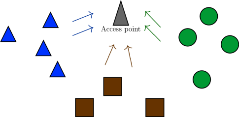
Figure 1: UMA with $T=3$ heterogeneous types of users.

Leveraging the natural heterogeneity and the maturity of SIC technique [38], we propose the decoder that employs power-domain NOMA [30, 31, 33, 32] at each slot. Specifically, without loss of generality, we assume the decoding order of power-domain NOMA in the physical layer is given by $1\rightarrow 2\rightarrow\ldots\rightarrow T$ and we define the intra-SIC decodable patterns as follows.

Definition 1.

(Type $t$ decodable pattern) For a slot $n\in[N]$, we define the transmission pattern $\mathbf{c}_{n}=(c_{1},\ldots,c_{T})$ to be a $T$-dimensional vector where the entry $c_{t}$ represents the total number of unresolved type $t$ packets at this slot. Such a vector $\mathbf{c}_{n}$ is type $t$ decodable if and only if the following conditions hold:

$$\text{(i) $c_{t}=1$},\quad\quad\quad\text{(ii) $c_{t^{\prime}}\leq 1$ for $t^{\prime}\in[t-1]$}$$

(iii) $$c_{\tilde{t}}\leq\tilde{t}-t \tilde{t}\in[t+1:T] \sum_{\tilde{t}=t+1}^{T}c_{\tilde{t}}\leq T-t$$ for ,(iv) .

The type $t$ decodable pattern is defined based on the principle of power-domain NOMA. In power-domain NOMA, it is assumed that a packet can be successfully decoded by intra-slot SIC as long as each interfered type has at most one packet collided at the same slot. This justifies the above conditions (i) and (ii). Moreover, types having later decoding order means that they will cause smaller interference. Therefore, trading a type $\tilde{t}\in[t+1:T]$ packet for a type $\hat{t}>\tilde{t}$ packet would not affect the decodability, justifying the conditions (iii) and (iv).

Definition 2.

(Type $t$ decodable set) The type $t$ decodable set $\mathcal{D}^{(t)}$ consists of all the type $t$ decodable patterns. i.e., $\mathcal{D}^{(t)}=\{\mathbf{c}:\mathbf{c}\leavevmode\nobreak\ \text{is type $t$ decodable}\}$.

Example 3.

When $T=2$, it is easy to check that $\mathcal{D}^{(1)}=\{(1,0),(1,1)\}$ and $\mathcal{D}^{(2)}=\{(0,1),(1,1)\}.$ When $T=3$, we have

$$\mathcal{D}^{(1)} =\{(1,0,0),(1,0,1),(1,0,2),(1,1,0),(1,1,1)\},$$ (1)

$$\mathcal{D}^{(2)} =\{(0,1,0),(0,1,1),(1,1,0),(1,1,1)\},$$ (2)

$$\mathcal{D}^{(3)} =\{(0,0,1),(0,1,1),(1,0,1),(1,1,1)\}.$$ (3)

The decoding process performed at the end of a frame then proceeds as follows. For every slot $n\in[N]$ during a frame, the corresponding transmission pattern $\mathbf{c}_{n}$ is computed. The intra-slot SIC is then employed to resolve a type $t$ packet if there is a $\mathbf{c}_{n}$ for $n\in[N]$ belonging to the type $t$ decodable set $\mathcal{D}^{(t)}$. We assume that in the burst payload of each packet, there is information about the (other) slots containing copies of this packet. Hence, the decoded packets are then used to cancel other replicas via inter-slot SIC. This completes an iteration and the decoding process continues iteratively until no more packets are decodable for all $t\in[T]$ and all $n\in[N]$ or all the packets in this frame are decoded. This process is done, independently, for every frame.

An example of the proposed IRSA with NOMA for $T=2$ can be found in Fig. 2. In this figure, the replicas of packets transmitted from the type 1 users, namely users 1 and 2, are colored in blue and that from the type 2 users, namely users 3 and 4, are colored in red. In this example, user 1’s packet can be easily decoded from slot 1. Subtracting user 1’s packet at slot 3 from the decoded packet, there’s no more degree-1 slot and traditional IRSA would stop the decoding process. For the proposed IRSA with NOMA, at slot 2, we receive the collision of a packet from type 1 (user 2) and another one from type 2 (user 4), both packets can be decoded via intra-slot SIC. Hence, our proposed IRSA with NOMA would continue the decoding process by subtracting users 2 and 4’s packets in slot 4 and decode user 4’s packet.

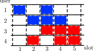
Figure 2: An example of SA with heterogeneous users transmitting in a frame of 5 slots. Here, we have $T=2$ types where the first type consists of users 1 and 2 and the second type consists of users 3 and 4.

At the end of the decoding process, suppose the base station can successfully decode $\hat{K}^{(t)}$ packets of type $t\in[T]$, we define the (actual) efficiency of type $t\in[T]$ achieved by the scheme as

$$\hat{\eta}^{(t)}=\frac{\hat{K}^{(t)}}{N},\quad t\in[T],$$ (4)

and the (actual) sum efficiency of the scheme as $\hat{\eta}=\sum_{i=1}^{T}\hat{\eta}^{(t)}.$ It is clear that choosing different $\mathcal{L}^{(t)}$ would result in different efficiency. Throughout the paper, we call a collection of $T$ degree distributions $\{\mathcal{L}^{(1)},\mathcal{L}^{(2)},\ldots,\mathcal{L}^{(T)}\}$, one for each type $t\in[T]$, a policy. The goal of this paper is then to design the policy, such that the achieved efficiency is maximized.

II-A Comparison with existing models

In this subsection, we discuss differences between the model considered in this paper and existing models.

Remark 4.

It is not difficult to see that when $T=1$, i.e., there is only one type of homogeneous users, the proposed protocol reduces to the IRSA protocol in [9]. In light of this, the proposed protocol can be regarded as a generalization of the IRSA protocol to accommodate heterogeneous types of users.

Remark 5.

We note that both multi-packet reception [34] and power-domain NOMA [30, 31, 32, 33] are based on the same physical-layer model, namely the multiple access channel [39]. However, the multi-packet reception technique treats all the users equally and assumes collided packets are decodable as long as the number of users collided at a slot is smaller than a predefined number. Hence, in this homogeneous setting, the problem in the physical layer becomes to establish reliable multiple access with homogeneous users that have the same codebook and code rate. To the best of our knowledge, this is not an easy task that is tackled with some success in [40] and [41], which involves either extremely large blocklength due to spatial coupling [40] or very complex operations of coding over prime fields. On the contrary, the power-domain NOMA lets the users transmit with different power levels and/or rates so that low-complex SIC can be employed to achieve a corner point of the capacity region. An illustration can be found in Fig. 3. In this paper, the considered problem exhibits natural heterogeneity among users; hence, it is more natural and suitable to work with power-domain NOMA so that the heterogeneity can be exploited by intra-SIC. The main theme of this paper then centers around analyzing policies for IRSA with power-domain NOMA and designing policies that optimally exploit the heterogeneity inherent in the considered problem.

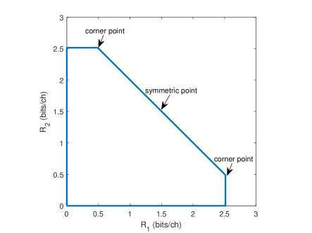
Figure 3: The capacity region of a two-user multiple access channel.

Remark 6.

The combination of NOMA and SA has been investigated before in [43, 44] by Choi. However, in these works, it is assumed that there is only one type of homogeneous users. The focus of [43] is mainly to analyze the performance of SA when users randomly choose their power levels and the receiver employs intra-slot SIC. Moreover, in both works [43, 44], the inter-slot SIC technique is not considered.

Remark 7.

We also note that our model is fundamentally different from IRSA with capture effect discussed in [9, Appendix A] and [45]. With capture effect, it is assumed that the receiver may be able to decode more than one packet with some probability. This opportunity usually comes from the effect of random channel fading. On the other hand, in the considered model, the receiver is able to decode more than one packet deterministically for certain configurations of collided users, due to the natural heterogeneity inherent in the problem.

II-B Implementation Issues

We now address potential implementation issues of the proposed IRSA with NOMA. We would like to note that many of these issues have been encountered and addressed by the conventional IRSA schemes [9]. However, we still present them here for the sake of self-containedness.

1. Slot synchronization: This issue is inherent in all slotted multiple access schemes. One easy solution to provide slot synchronization is to rely on stable clocks and a small amount of guard time between packets [5, Sec. 4.2]. Moreover, for applications with cheap user devices, stable clocks may be unaffordable. For such scenarios, [46] provides a technique to achieve slot synchronization, where each node constantly re-synchronizes its clock with the base station by exploiting the ACK signals fed back from the base station. Another source of slot synchronization errors which is less seen in traditional communication systems is from significantly different travel distances experienced by different devices’ signals. This type of source of slot synchronization errors has become important in non-terrestrial networks (NTN) [47]. Fortunately, in NTN, each device is required to be GNSS-capable for acquiring its own position and together with satellite ephemeris. Each user can calculate and then pre-compensate its timing advance (TA) (see Section 6.3 in [47]). To reduce devices’ computation loading, another candidate technique currently under discussion in 3GPP is that the base station estimates and broadcasts TA to a group of devices who have similar TA (see Section 6.3 in [47]).

2. Frame synchronization: This issue is also not new and has to be cope with in every frame-synchronous systems. This issue can be addressed by letting the base station periodically broadcasting a beacon signal at the beginning of each frame. In Section VI, extension to frame asynchronous setting will be discussed.

3. Inter-slot SIC: Similar to CRDSA [7] and IRSA schemes [9], to enable inter-slot SIC, the proposed protocol requires the knowledge of the locations of other replicas once a packet is successfully decoded. This can be achieved by including pointers to the locations of other replicas into the burst payload or by some pseudo-random mechanism known by both the transmit and receive ends. For example, the DVB system [8] adopts the latter one, where each active user reports its MAC address and a pseudo-random number to the base station. Both the base station and the user can then compute the slots used for sending replicas by a common deterministic function of the MAC address and the pseudo-random number.

4. Intra-slot SIC: For the proposed scheme, in order to enable intra-slot SIC at a slot, it appears that the receiver has to know which types of packets are collided in this slot. This issue is new in our proposed protocol. We provide two ways to address this issue. We note that in DVB-RCS2 [8], each active user selects the number of transmissions and a random seed for uniquely determining a pseudo random pattern. This information is then stored in the burst payload and sent to the base station. Given the existing data structure, to enable intra-slot SIC, each user can include additional $\log(T)$ bits to the payload for revealing its type. The second method described in the sequel eliminates the need for sending extra $\log(T)$ bits by increasing the decoding burden. Let $R^{(t)}$ be the rate of the physical-layer channel code adopted by users of type $t\in[T]$. Let us assume the We assume that the rate tuple $(R^{(1)},R^{(2)},\ldots,R^{(T)})$ can be achieved by intra-slot SIC with ascending decoding order $1\rightarrow 2\rightarrow\ldots\rightarrow T$, without loss of generality. Following the NOMA principle, a means to address this issue is as follows: Starting from $t=1$, the base station tries to decode a packet of type $t$; if it succeeds, the decoded packet is subtracted from the received signal and we set $t=t+1$; otherwise, directly set $t=t+1$ and look for decoding opportunity of the next type. This procedure would continue until $t=T$.

III Graph Representation

In this section, we introduce a graph representation of the proposed IRSA with NOMA protocol for determining an optimal policy in Section IV.

III-A Bipartite Graph and Degree Distributions

We first note that in UMA with $T$ types of heterogeneous users, each type has its own transmission policy and number of users that may be different from other types. We construct a bipartite graph representation of the proposed IRSA with NOMA protocol. The graph consists of $\sum_{t=1}^{T}K^{(t)}$ variable nodes and $N$ super check nodes, as shown in Fig. 4. Each variable node $\mathsf{v}^{(t)}_{j}$ represents a user $j\in[K^{(t)}]$ of type $t\in[T]$. Each super check node consists of $T$ check nodes $\mathsf{c}^{(t)}_{n}$, one for each type $t\in[T]$. A user $j$ of type $t\in[T]$ transmits a packet in slot $n\in[N]$ if and only if there is an edge connecting $\mathsf{v}^{(t)}_{j}$ with $\mathsf{c}^{(t)}_{n}$. For simplicity, we use $\mathsf{v}^{(t)}$ and $\mathsf{c}^{(t)}$ to denote a generic variable and check nodes of type $t\in[T]$.

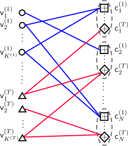
Figure 4: A bipartite graph representation of the proposed IRSA with NOMA.

With this bipartite graph representation, a user of type $t$ who transmits $d$ replicas corresponds to a degree $d$ variable node $\mathsf{v}^{(t)}$. Moreover, a time slot in which $d$ type $t$ variable nodes transmit corresponds to a degree $d$ check node $\mathsf{c}^{(t)}$. We define the node perspective left and right degree distributions as

$$\mathcal{L}^{(t)}[x]=\sum_{d}L^{(t)}_{d}x^{d}\quad\text{and}\quad\mathcal{R}^{(t)}[x]=\sum_{d}R^{(t)}_{d}x^{d},$$ (5)

respectively, where $L^{(t)}_{d}$ is the probability that a variable node $\mathsf{v}^{(t)}$ has degree $d$ and $R^{(t)}_{d}$ is the probability that a check node $\mathsf{c}^{(t)}$ has degree $d$. Through the node perspective degree distributions, the edge perspective left and right degree distributions can be given by

$$\lambda^{(t)}[x]=\sum_{d}\lambda^{(t)}_{d}x^{d-1}=\frac{\mathcal{L}^{{}^{\prime}(t)}[x]}{\mathcal{L}^{{}^{\prime}(t)}[1]},$$ (6)

and

$$\rho^{(t)}[x] =\sum_{d}\rho^{(t)}_{d}x^{d-1}=\frac{\mathcal{R}^{{}^{\prime}(t)}[x]}{\mathcal{R}^{{}^{\prime}(t)}[1]},$$ (7)

respectively, where $\lambda^{(t)}_{d}$ stands for the probability that an edge connects to a type $t$ variable node of degree $d$ and $\rho^{(t)}_{d}$ is the probability that an edge connects to a type $t$ check node of degree $d$.

The target efficiency of type $t\in[T]$ is then defined as

$$\eta^{(t)}=\frac{K^{(t)}}{N}=\frac{\mathcal{R}^{{}^{\prime}(t)}[1]}{\mathcal{L}^{{}^{\prime}(t)}[1]},$$ (8)

and the target sum efficiency of the scheme is defined as $\eta=\sum_{t=1}^{T}\eta^{(t)}.$ Note that the target efficiency $\eta^{(t)}$ is different from the actual efficiency $\hat{\eta}^{(t)}$ in (4). In general, $\hat{\eta}^{(t)}\leq\eta^{(t)}$ with equality if and only if all packets are successfully decoded.

Example 8.

Consider the scheme described in Fig. 2 where there is one type 1 variable node of degree 2 and one type 1 variable node of degree 3. Hence, $\mathcal{L}^{(1)}[x]=0.5x^{2}+0.5x^{3}$. One can obtain $\mathcal{L}^{(2)}[x]=x^{3}$ in a similar fashion. Also, there are three type 1 check nodes of degree 1 and one type 1 check node of degree 2. Therefore, $\mathcal{R}^{(1)}[x]=0.75x+0.25x^{2}$. Similarly, $\mathcal{R}^{(2)}[x]=0.5x+0.5x^{2}.$ Moreover, one can easily verify that the edge perspective degree distributions are given by

$$\lambda^{(1)}[x]=\frac{2}{5}x+\frac{3}{5}x^{2},\quad\lambda^{(2)}[x]=x^{2},\quad\rho^{(1)}[x]=\frac{3}{5}+\frac{2}{5}x,\quad\rho^{(2)}[x]=\frac{1}{3}+\frac{2}{3}x.$$ (9)

The graph representation of this example can be found in Fig. 5-(a).

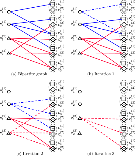
Figure 5: The graph representation of the scheme in Fig. 2 and its decoding output at each iteration of the modified peeling decoder.

III-B Modified Peeling Decoder

Here, we propose a modified peeling decoder for the bipartite graph that corresponds to the decoding procedure of the proposed IRSA with NOMA. The decoder operates in an iterative fashion. For each iteration, the decoder looks at every super check node $n\in[N]$ and computes the remaining degrees of check nodes $\mathsf{c}^{(t)}_{1},\mathsf{c}^{(t)}_{2},\ldots,\mathsf{c}^{(t)}_{T}$, which are stored in the transmission pattern $\mathbf{c}_{n}$. We then look for an $n$ such that $\mathbf{c}_{n}$ belongs to the type $t$ decodable set $\mathcal{D}^{(t)}$ for some $t\in[T]$. If such an $n$ exists, we use intra-slot SIC to decode all the type $t$ packets satisfying $\mathbf{c}_{n}\in\mathcal{D}^{(t)}$ in this super check node $n$. For a variable node $\mathsf{v}^{(t)}$ that is decoded, all the edges connected with it are removed from the graph. This concludes an iteration. The modified peeling decoder operates iteratively until no more decoding opportunity is found.

Example 8 (continued).

In this example, we illustrate how to use the modified peeling decoder to decode the scheme in Example 8. As shown in Fig. 5-(b), in iteration 1, $\mathsf{c}^{(1)}_{1}$ has degree 1 and $\mathsf{c}^{(2)}_{1}$ has degree 0, i.e., $\mathbf{c}_{1}=(1,0)\in\mathcal{D}^{(1)}$; hence, $\mathsf{v}^{(1)}_{1}$ is decoded and all its edges are removed. Then, in iteration 2 shown in Fig. 5-(c), $\mathsf{c}^{(1)}_{2}$ has degree 1 and $\mathsf{c}^{(2)}_{2}$ has degree 1, i.e., $\mathbf{c}_{2}=(1,1)$ belonging to both $\mathcal{D}^{(1)}$ and $\mathcal{D}^{(2)}$; thus, both $\mathsf{v}^{(1)}_{2}$ and $\mathsf{v}^{(2)}_{2}$ can be decoded by intra-slot SIC. All the edges connected to $\mathsf{v}^{(1)}_{2}$ and $\mathsf{v}^{(2)}_{2}$ are subsequently removed. Last, in iteration 3 shown in Fig. 5-(d), one can easily see that $\mathsf{v}^{(2)}_{1}$ can be decoded.

IV Multi-Dimensional Density Evolution and Convergence Analysis

In this section, to analyze the IRSA with NOMA, we propose a novel multi-dimensional density evolution based on the graph representation described in Section III. With this multi-dimensional density evolution, we then provide the convergence analysis of the IRSA with NOMA under modified peeling decoding. With an assist from the convergence analysis, we formulate and numerically solve an optimization problem that finds best left degree distributions, leading to the highest asymptotic efficiency. For clearly explaining the ideas behind our scheme and analysis, we focus on $T=2$. The general $T$ case can be similarly analyzed.

IV-A Proposed Multi-Dimensional Density Evolution

It is well known that for LDPC codes over a binary erasure channel, BP and peeling decoders have the same performance. Moreover, density evolution is an outstanding tool for analyzing the performance of BP decoding over a sparse graph [10]. Thus, this section proposes a novel multi-dimensional density evolution to analyze the performance of the proposed scheme under BP decoding. Similar to that introduced in [10, Sec. 2.5], the BP decoding is an iterative algorithm where in each iteration, each variable node computes the belief of its own message and passes an extrinsic version of it to each connected check node, while each check node computes its belief of the message of each connected variable node and passes an extrinsic version to that variable node. After a predefined number of iterations, the decoding algorithm halts and outputs hard decisions according to the last beliefs held by the variable nodes.

Consider BP decoding described above. For $t\in[2]$, we denote by $x_{\ell}^{(t)}$ and $y_{\ell}^{(t)}$ the average erasure probability of the message passed along an edge from $\mathsf{v}^{(t)}$ to $\mathsf{c}^{(t)}$ and that of the message passed along an edge from $\mathsf{c}^{(t)}$ to $\mathsf{v}^{(t)}$ in iteration $\ell$, respectively. At iteration $\ell=0$, according to the decodable set $\mathcal{D}^{(t)}$ specified in Example 3, for an edge connected to a type $t$ check node $\mathsf{c}^{(t)}$, the outgoing message is not in erasure if and only if a) $\mathsf{c}^{(t)}$ has degree 1; b) $\mathsf{c}^{(\bar{t})}$ has a degree either 0 or 1 for every $\bar{t}\in[2],\leavevmode\nobreak\ \bar{t}\neq t$. Hence, we initialize $y_{0}^{(t)}$ for initial iteration $\ell=0$ to be

$$y_{0}^{(t)}=1-\rho^{(t)}[0]\cdot\left(\mathcal{R}^{(\bar{t})}[0]+\mathcal{R}^{{}^{\prime}(\bar{t})}[0]\right),$$ (10)

where $\mathcal{R}^{(\bar{t})}[0]=R^{(\bar{t})}_{0}$ and $\mathcal{R}^{{}^{\prime}(\bar{t})}[0]=R^{(\bar{t})}_{1}$ are the fractions of type $\bar{t}$ check nodes having degree 0 and degree 1, respectively. Moreover, the term $\rho^{(t)}[0]=\rho_{1}^{(t)}$ is the probability that an edge connects to a type $t$ check node of degree $1$.

Suppose we have obtained $x_{\ell}^{(t)}$ and $y_{\ell}^{(t)}$ for all $t\in[T]$ from iteration $\ell$. In iteration $\ell+1$, for an edge incident to a variable node $\mathsf{v}^{(t)}$ with degree $d$, the only possibility that the message along this edge to a $\mathsf{c}^{(t)}$ is in erasure is that all the other $d-1$ edges are in erasure. Therefore, the probability that the message passed along this edge is in erasure is $(y_{\ell}^{(t)})^{d-1}$. Now, averaging over all the edges results in the average erasure probability

$$x_{\ell}^{(t)}=\sum_{d}\lambda^{(t)}_{d}(y_{\ell}^{(t)})^{d-1}=\lambda^{(t)}[y_{\ell}^{(t)}].$$ (11)

For an edge incident to a check node $\mathsf{c}^{(t)}$ with degree $d$, the message passed along this edge to a $\mathsf{v}^{(t)}$ is not in erasure if and only if a) all the other $d-1$ edges incident to $\mathsf{c}^{(t)}$ are not in erasure in the previous iteration; and b) all but at most one of the edges incident to $\mathsf{c}^{(\bar{t})}$ are not in erasure in the previous iteration for every $\bar{t}\in[2],\leavevmode\nobreak\ \bar{t}\neq t$. Suppose in the same super check node $n$, $\mathsf{c}^{(\bar{t})}_{n}$ has degree $d_{\bar{t}}$. Then the above event has probability

$$(1-x_{\ell}^{(t)})^{d-1}\cdot\left((1-x_{\ell}^{(\bar{t})})^{d_{\bar{t}}}+d_{\bar{t}}x_{\ell}^{(\bar{t})}(1-x_{\ell}^{(\bar{t})})^{d_{\bar{t}}-1}\right),$$ (12)

where $(1-x_{\ell}^{(\bar{t})})^{d_{\bar{t}}}$ is the probability that all $d_{\bar{t}}$ edges are not erased and $d_{\bar{t}}x_{\ell}^{(\bar{t})}(1-x_{\ell}^{(\bar{t})})^{d_{\bar{t}}-1}$ is the probability that all but one edges are not erased. Now, averaging over all the edges and over all the type $\bar{t}$ check nodes for $\bar{t}\in[2],\leavevmode\nobreak\ \bar{t}\neq t$ shows that the average probability of correct decoding is given by

$$\sum_{d}\lambda^{(t)}_{d}(1-x_{\ell}^{(t)})^{d-1}\cdot\sum_{d_{\bar{t}}}R^{(\bar{t})}_{d_{\bar{t}}}\left((1-x_{\ell}^{(\bar{t})})^{d_{\bar{t}}}+d_{\bar{t}}x_{\ell}^{(\bar{t})}(1-x_{\ell}^{(\bar{t})})^{d_{\bar{t}}-1}\right)$$

$$=\rho^{(t)}[1-x_{\ell}^{(t)}]\left(\mathcal{R}^{(\bar{t})}[1-x_{\ell}^{(\bar{t})}]+x_{\ell}^{(\bar{t})}\mathcal{R}^{{}^{\prime}(\bar{t})}[1-x_{\ell}^{(\bar{t})}]\right).$$ (13)

Therefore, the average erasure probability becomes

$$y_{\ell+1}^{(t)}=1-\rho^{(t)}[1-x_{\ell}^{(t)}]\cdot\left(\mathcal{R}^{(\bar{t})}[1-x_{\ell}^{(\bar{t})}]+x_{\ell}^{(\bar{t})}\mathcal{R}^{{}^{\prime}(\bar{t})}[1-x_{\ell}^{(\bar{t})}]\right).$$ (14)

Plugging (11) into (14) leads to the evolution of average erasure probability of a type $t$ check node as shown in (15) in the bottom of next page.

$$y_{\ell+1}^{(t)}=1-\rho^{(t)}[1-\lambda^{(t)}[y_{\ell}^{(t)}]]\cdot\left(\mathcal{R}^{(\bar{t})}[1-\lambda^{(\bar{t})}[y_{\ell}^{(\bar{t})}]]+\lambda^{(\bar{t})}[y_{\ell}^{(\bar{t})}]\mathcal{R}^{{}^{\prime}(\bar{t})}[1-\lambda^{(\bar{t})}[y_{\ell}^{(\bar{t})}]]\right),\quad t\in[2].$$ (15)

IV-B Convergence and Stability Condition

After obtaining the density evolution in (15), for any given degree distributions $\mathcal{L}^{(t)}$ (or $\lambda^{(t)}$) and $\mathcal{R}^{(t)}$ (or $\rho^{(t)}$), one can now analyze whether the average erasure probability converges to 0 by checking whether $y_{\ell}^{(t)}>y_{\ell+1}^{(t)}$ for every $\ell$, starting from $y_{0}^{(t)}=1$ for $t\in[T]$.

Moreover, to make sure that the average erasure probability indeed vanishes instead of hovering around 0, we derive the following stability condition. We enforce $\lambda_{1}^{(t)}=0$ for all $t\in[2]$ because we certainly do not want degree 1 variable nodes. Then, assuming $y^{(t)}$ is very small for all $t\in[2]$, we expand the degree distributions and approximate them by keeping only the linear terms as follows,

$$\lambda^{(t)}[y^{(t)}] \approx\lambda_{2}^{(t)}y^{(t)},$$ (16)

$$\rho^{(t)}[1-\lambda^{(t)}[y^{(t)}]] \approx 1-\rho^{{}^{\prime}{(t)}}[1]\lambda_{2}^{(t)}y^{(t)},$$ (17)

$$R^{(\bar{t})}[1-\lambda^{(\bar{t})}[y^{(\bar{t})}]] \approx 1-R^{{}^{\prime}(\bar{t})}[1]\lambda_{2}^{(\bar{t})}y^{(\bar{t})},$$ (18)

$$R^{{}^{\prime}(\bar{t})}[1-\lambda^{(\bar{t})}[y^{(\bar{t})}]] \approx R^{{}^{\prime}(\bar{t})}[1]-R^{{}^{\prime\prime}(\bar{t})}[1]\lambda_{2}^{(\bar{t})}y^{(\bar{t})}.$$ (19)

We can now linearize the recursion around 0 by plugging (16)-(19) into (15) to get

$$y^{(t)}>1-(1-\rho^{{}^{\prime}{(t)}}[1]\lambda_{2}^{(t)}y^{(t)})\left(1-R^{{}^{\prime\prime}(\bar{t})}[1](\lambda_{2}^{(t)}y^{(\bar{t})})^{2}\right)\approx\rho^{{}^{\prime}{(t)}}[1]\lambda_{2}^{(t)}y^{(t)},$$ (20)

which leads to the following stability condition

$$\lambda_{2}^{(t)}<\frac{1}{\rho^{{}^{\prime}{(t)}}[1]}\quad\text{for $t\in[2]$}.$$ (21)

IV-C Optimization Problem

Before we formulate the optimization problem, we note that there are two sets of degree distributions $\{\mathcal{L}^{(t)}[x]\}$ and $\{\mathcal{R}^{(t)}[x]\}$ in the proposed problem, but we only have control over $\{\mathcal{L}^{(t)}[x]\}$. The behavior of $\{\mathcal{R}^{(t)}[x]\}$; however, are completely determined by how the users behave. Specifically, according to the protocol, a type $t$ user $\mathsf{v}^{(t)}$ having degree $L$ will send a replica in slot $\mathsf{c}^{(t)}$ with probability $L/N$. Hence the average probability that a user $\mathsf{v}^{(t)}$ sending a replica in slot $\mathsf{c}^{(t)}$ is given by $\frac{\mathcal{L}^{{}^{\prime}(t)}[1]}{N}=\frac{\mathcal{R}^{{}^{\prime}(t)}[1]}{K^{(t)}}.$ Thus, the degrees of $\mathsf{c}^{(t)}$ follows the Binomial distribution with parameter $\frac{\mathcal{L}^{{}^{\prime}(t)}[1]}{N}$. Similar to [9], by Poisson approximation [49], we have

$$\mathcal{R}^{(t)}[x]\approx\exp\left(-\mathcal{R}^{{}^{\prime}(t)}[1](1-x)\right)=\exp\left(-\eta^{(t)}\mathcal{L}^{{}^{\prime}(t)}[1](1-x)\right).$$ (22)

Moreover, from (6), we have

$$\rho^{(t)}[x]=\exp\left(-\eta^{(t)}\mathcal{L}^{{}^{\prime}(t)}[1](1-x)\right).$$ (23)

Now, the convergence condition becomes (IV-C) in the bottom of the this page by plugging (23) into (15) and noting that it is sufficient that $y^{(t)}_{\ell+1}<y^{(t)}_{\ell}$ for every $\ell$ with $y^{(t)}_{\ell}\neq 0$.

$$y_{\ell}^{(t)}>1-\exp\left(-\eta^{(t)}\mathcal{L}^{{}^{\prime}(t)}[1]\lambda^{(t)}[y_{\ell}^{(t)}]\right)\cdot$$

$$\left(\exp\left(-\eta^{(\bar{t})}\mathcal{L}^{{}^{\prime}(\bar{t})}[1]\lambda^{(\bar{t})}[y_{\ell}^{(\bar{t})}]\right)+\eta^{(\bar{t})}\mathcal{L}^{{}^{\prime}(\bar{t})}[1]\lambda^{(\bar{t})}[y_{\ell}^{(\bar{t})}]\exp\left(-\eta^{(\bar{t})}\mathcal{L}^{{}^{\prime}(\bar{t})}[1]\lambda^{(\bar{t})}[y_{\ell}^{(\bar{t})}]\right)\right),\quad t\in[2].$$ (24)

Now, we are ready to formulate the optimization problem that maximizes the target efficiency subject to conditions derived thus far:

$$\!\max_{\{\mathcal{L}^{(t)}[x]\}} \eta=\sum_{t=1}^{2}\eta^{(t)}$$

subject to $$\text{convergence condition\leavevmode\nobreak\ }\eqref{eqn:DE_full_poisson},$$

$$\lambda_{1}^{(t)}=0\leavevmode\nobreak\ \text{for $t\in[2]$},$$

$$L_{d}^{(t)}\geq 0,\leavevmode\nobreak\ \text{for $d\in[d_{\mathrm{max}}^{(t)}]$ and $t\in[2]$},$$

$$\mathcal{L}^{(t)}[1]=1\leavevmode\nobreak\ \text{for $t\in[2]$},$$

where $d_{\mathrm{max}}^{(t)}$ is the maximum degree of $\mathcal{L}^{(t)}[x]$ that has to be imposed in practice. We solve this problem and provide some optimized degree distributions in the next subsection. We note that the stability condition (21) is not strictly required for maximizing the target efficiency as above. However, for applications that require very low packet loss rates, we do need to include (21) into our optimization problem in order to make sure that the average erasure probability does vanish.

IV-D Solving the Optimization Problem

In what follows, we again focus on $T=2$ solely but the discussion and intuitions apply to any $T\geq 2$. For $T=2$, let $y^{(t)}$ and $y^{(t)^{\prime}}$ be the LHS and RHS of (IV-C), representing the average erasure probability before and that after an iteration, respectively. Similar to the conventional IRSA in [9], we can have a sufficient condition for decodability that $y^{(t)^{\prime}}<y^{(t)}$ for $t\in[2]$ and every $(y^{(1)},y^{(2)})\in(0,1]\times(0,1]$. This admits a graphical interpretation as follows. Note that it is a $T=2$ dimensional problem and we need a curve of $(y^{(1)^{\prime}},y^{(2)^{\prime}})$ against $(y^{(1)},y^{(2)})$, which is in 4 dimensional space. We instead plot $y^{(1)^{\prime}}$ against $(y^{(1)},y^{(2)})$ and $y^{(2)^{\prime}}$ against $(y^{(1)},y^{(2)})$ separately in Figs 6(a) and 6(b), respectively. In Fig. 6(a), the identity plane is the hyperplane consisting of $(y^{(1)},y^{(2)},y^{(1)})$ and the evolution plane for the degree distribution pair $\mathsf{P}_{2}$ shown in Table I consists of $(y^{(1)},y^{(2)},y^{(1)^{\prime}})$. Similarly, in Fig. 6(b), we show the identity plane consisting of $(y^{(1)},y^{(2)},y^{(2)})$ and also plot the evolution plane for $\mathsf{P}_{2}$ that consists of $(y^{(1)},y^{(2)},y^{(2)^{\prime}})$. The sufficient condition mentioned above is then to ask the entire evolution plane lie beneath the identity plane in both figures. However, this is by no means necessary and is way too strong as after each iteration, both $y^{(1)}$ and $y^{(2)}$ drop and some pairs like $(0,1)$ and $(1,0)$ will never be visited. Also shown in Figs. 6(a) and 6(b) is the evolution path of the considered distribution pair that is generated by using the output $(y^{(1)^{\prime}},y^{(2)^{\prime}})$ of the previous iteration as input. This evolution path depicts the trajectory of the pair of erasure probabilities evolving with the iterative decoding algorithm. Although the evolution plane does not lie entirely beneath the identity plane, since the evolution path in this example lies entirely beneath the identity plane and has the unique fixed point at the origin, this degree distribution pair is decodable.

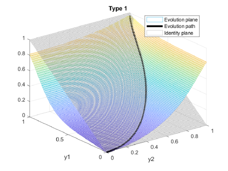
(a) Type 1: $y^{(1)^{\prime}}$.

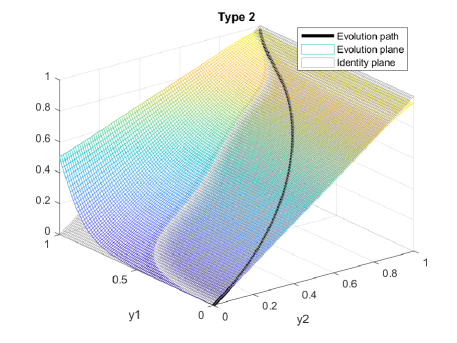
(b) Type 2: $y^{(2)^{\prime}}$.

Figure 6: Identity plane, evolution plane, and evolution path

With the above observation, we propose a new sufficient condition for a degree distribution pair to be decodable: There exists an evolution path that lies entirely beneath the identity plane. Hence, the optimization problem becomes to find a degree distribution pair with the evolution path all but touches the identity plane. We then adopt the differential evolution technique [50] to solve this optimization problem. Specifically, in the mutation step of differential evolution, we adopt the DEEP algorithm in [51] and use the “bounce-back” method [50, Chapter 4.3.1] to handle the boundary conditions. Some optimized degree distributions $\mathcal{L}^{(t)}[x]$ with $d_{\mathrm{max}}^{(t)}=8$ for $t\in[T]$ are shown in Table I. In addition, the corresponding thresholds $\eta^{*}$, the analytic result of $\eta$ in the limit as $N\rightarrow\infty$, are also shown. In this table, the policies $\mathsf{P}_{1}$, $\mathsf{P}_{2}$, and $\mathsf{P}_{3}$ are produced by solving the above optimization problem for the cases when $K^{(1)}=K^{(2)}$, $3K^{(1)}=K^{(2)}$, and $7K^{(1)}=K^{(2)}$, respectively. We also provide an example with $T=3$ whose density evolution and the corresponding optimization problem can be found in Appendix A. The policy $\mathsf{P}_{4}$ provides a set of optimized degree distributions for $T=3$ with $K^{(1)}=K^{(2)}=K^{(3)}$. Finally, the policy $\mathsf{P}_{5}$ is that for conventional IRSA with $T=1$ and is directly borrowed from [9]. These policies will be tested with simulations in the next section.

Remark 9.

From Table I, one can observe that every proposed policy has an threshold larger than $100\%$. At first glance, this seems violating the fundamental limit of UMA that at most 1 packet can be successfully delivered in 1 slot, even under perfect coordination. However, we would like to stress that this is not the fundamental limit for our setting, as in our protocol, leveraging heterogeneity among users, it is entirely possible that one can use intra-SIC to decode at most $T$ packets in a slot.

Remark 10.

It is worth mentioning that for $T=2$, when the numbers of active users of type $t\in[2]$ are the same, the optimized degree distributions $\mathcal{L}^{(t)}[x]$ become the same for $t\in[2]$. See for e.g. $\mathsf{P}_{1}$ in Table I. This makes perfect sense as when $K^{(1)}=K^{(2)}$, the decodable sets $\mathcal{D}^{(1)}$ and $\mathcal{D}^{(2)}$ become symmetric as shown in Example 3. However, when $T=3$, the degree distributions become different. This can also be explained by the different decodable sets in Example 3.

Table I: Optimized degree distributions and thresholds

Policy	$T$	$\mathcal{L}^{(t)}[x]$	$\eta^{*}$
$\mathsf{P}_{1}$	2	$\mathcal{L}^{(1)}[x]=0.665x^{2}+0.1515x^{3}+0.1835x^{8}$ $\mathcal{L}^{(2)}[x]=0.665x^{2}+0.1515x^{3}+0.1835x^{8}$	$1.433$
$\mathsf{P}_{2}$	2	$\mathcal{L}^{(1)}[x]=0.3305x^{2}+0.0165x^{4}+0.0019x^{5}+0.01825x^{6}+0.0141x^{7}+0.4545x^{8}$ $\mathcal{L}^{(2)}[x]=0.4910x^{2}+0.3145x^{3}+0.0028x^{5}+0.0029x^{6}+0.0287x^{7}+0.1601x^{8}$	$1.232$
$\mathsf{P}_{3}$	2	$\mathcal{L}^{(1)}[x]=0.9388x^{2}+0.0032x^{4}+0.058x^{5}$ $\mathcal{L}^{(2)}[x]=0.508x^{2}+0.276x^{3}+0.216x^{8}$	$1.064$
$\mathsf{P}_{4}$	3	$\mathcal{L}^{(1)}[x]=0.746x^{2}+0.093x^{3}+0.161x^{8}$ $\mathcal{L}^{(2)}[x]=0.7507x^{2}+0.0846x^{3}+0.1647x^{8}$ $\mathcal{L}^{(3)}[x]=0.7507x^{2}+0.0846x^{3}+0.1647x^{8}$	$1.851$
$\mathsf{P}_{5}$	1	$\mathcal{L}^{(1)}[x]=0.5x^{2}+0.28x^{3}+0.22x^{8}$ [9]	$0.938$

V Simulation Results

In this section, we validate the proposed IRSA with NOMA via extensive simulations under practical frame sizes. In particular, to demonstrate the effectiveness of the proposed method, we will use the efficiency $\hat{\eta}$ versus the total active users per slot, $\sum_{t=1}^{N}K^{(t)}/N$ (that is $\eta$), as the metric.

In Fig. 7, we compare the achieved efficiency of the proposed IRSA with NOMA for different $T$. Specifically, in Fig. 7, for both $N=150$ and $1500$, we compare the efficiencies of $\mathsf{P}_{5}$, $\mathsf{P}_{1}$, and $\mathsf{P}_{4}$, that are optimized for $T=1$, $T=2$, and $T=3$, respectively. From these figures, we can observe that the proposed multi-dimensional density evolution indeed accurately predicts the efficiency of the proposed IRSA with NOMA as $N$ increases. Moreover, we observe that the more types, the higher efficiency the proposed algorithm can achieve. The proposed multi-dimensional density evolution predicts an efficiency of $143\%$ for $\mathsf{P}_{1}$ and $185\%$ for $\mathsf{P}_{4}$, which are both significantly higher than the $93.8\%$ achieved by the conventional IRSA with $\mathsf{P}_{5}$. This indicates that when the application at hand presents natural heterogeneity, the proposed IRSA with NOMA can effectively exploit it.

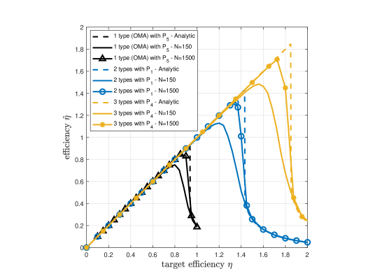
Figure 7: Efficiency versus target efficiency (active users per slot) at $N=150$ and $1500$ for $\mathsf{P}_{5}$ ($T=1$), $\mathsf{P}_{1}$ ($T=2$), and $\mathsf{P}_{4}$ ($T=3$).

In Fig. 8, we show the efficiency of the proposed IRSA with NOMA for $T=2$ where the two groups have different numbers of users. Again, for both $N=150$ and $1500$, we plot the efficiencies of $\mathsf{P}_{1}$, $\mathsf{P}_{2}$, and $\mathsf{P}_{3}$, that are optimized for the cases $K^{(1)}=K^{(2)}$, $3K^{(1)}=K^{(2)}$, and $7K^{(1)}=K^{(2)}$, respectively. One can see from this figure that the larger the difference between the numbers of users, the smaller efficiency. This is because the small difference means that the number of users in a group is roughly the same from group to group; thereby, it means the heterogeneity is large and more decoding opportunity may be introduced by intra-slot SIC. On the contrary, if the difference is large, it means that one of the group contains most of the users in the network; hence, heterogeneity is small. An extreme example can be seen by considering $M\cdot K^{(1)}=K^{(2)}$ and let $M\rightarrow\infty$, under which the problem would become the homogeneous setting and no heterogeneity can be exploited.

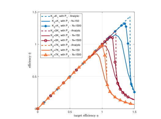
Figure 8: Efficiency versus target efficiency (active users per slot) at $N=150$ and $1500$ for $\mathsf{P}_{1}$ ($K^{(1)}=K^{(2)}$), $\mathsf{P}_{2}$ ($K^{(1)}=3K^{(2)}$), and $\mathsf{P}_{3}$ ($K^{(1)}=7K^{(2)}$).

Figs. 7 and 8 have demonstrated that thanks to NOMA, the proposed protocol can efficiently exploit the heterogeneity inherent in the network. One natural question arising at this point is whether this gain comes solely from the intrinsic benefit of NOMA or the analysis and optimization proposed in Sections IV-A and IV-C indeed play a role. In other words, do the optimized policies in Table I indeed provide non-negligible gains over $\mathsf{P}_{5}$ when $T=2$ and $T=3$? We note that with a larger decodable set enabled by intra-slot SIC, each node should transmit less in order to maintain the same chance to be successfully decoded while reducing the probability of causing unresolvable collisions. However, $\mathsf{P}_{5}$ is optimized for $T=1$ [9], which do not take the larger decodable set into account. Hence, nodes adopting this distribution would tend to over-transmit. To confirm this, we look into the degree distributions and observe that the average degrees are 3.6, 3.25, and 3.068 for $\mathsf{P}_{5}$, $\mathsf{P}_{1}$, and $\mathsf{P}_{4}$, respectively. Moreover, for the optimized degree distributions, as $T$ increases, the fraction of degree 2 nodes increases while that of degrees 3 and 8 nodes decreases. In Fig. 9, we compare the performance of $\mathsf{P}_{5}$ optimized for $T=1$ and the respective optimized degree distributions at $N=150$. The analytic results obtained by the multi-dimensional density evolution are also plotted, which indicate that the optimized degree distributions provide efficiency gains of 0.083 and 0.174 over $\mathsf{P}_{5}$ when $T=2$ and $T=3$, respectively. Simulation results also show similar gains, which corroborate our analysis. This gain of the optimized degree distribution over $\mathsf{P}_{5}$ is expected to increase as $T$ increases due to the larger and larger decodable set.

In contrast, when the numbers of users of different types are drastically different, the gain of the optimized degree distribution over $\mathsf{P}_{5}$ becomes negligible. For such a scenario, we end up focusing more and more on the type with the largest size and the optimized degree distribution becomes more and more like $\mathsf{P}_{5}$. This is evident by observing that $\mathsf{P}_{5}$ and $\Lambda^{(2)}$ (for the type that is 7 times larger than the other) in $\mathsf{P}_{3}$ are very similar to each other and that the density evolution shows almost identical efficiency. That said, the optimized degree distribution still enjoys a significantly less average degree of 2.89 as opposed to 3.6 in $\mathsf{P}_{5}$.

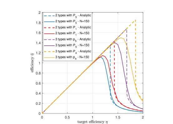
Figure 9: Comparison of the suboptimal policy ($\mathsf{P}_{5}$) and the optimized policy ($\mathsf{P}_{1}$ when $T=2$ and $\mathsf{P}_{4}$ when $T=3$) at $N=150$.

VI Extension to Frame Asynchronous Case

In this section, we extend the proposed IRSA with NOMA and the corresponding multi-dimensional density evolution to the frame asynchronous setting. Both the analysis and the simulation results indicate that similar to [16], such asynchrony results in the boundary effect [17] that facilitates our system design by enabling easily implemented regular left degrees to be asymptotically optimal. Moreover, since there is no concept of frame, the users do not have to wait until the next frame and can immediately start the transmission upon the arrival of a packet.

VI-A Problem and Protocol

In the frame asynchronous setting, the users are allowed to join the network without frame synchronization; but slots are still synchronous. We assume that the arrival of type $t$ users’ data follows a Poisson distribution with arrival rate $g^{(t)}$. That is, the probability that $m^{(t)}$ type $t$ users join the system in a given slot is given by $\frac{\exp(-g^{(t)})(g^{(t)})^{m^{(t)}}}{m^{(t)}!}.$ We note here that $g^{(t)}$ has the unit “users per slot” and plays a similar role with the target efficiency $\eta^{(t)}$ in the frame synchronous setting. Also, the sum arrival rate $g=\sum_{t=1}^{T}g^{(t)}$ plays a similar role with $\eta$ in the frame synchronous setting. Under this frame asynchronous setting, each user has its local view about “frame” of size $N$ slots starting from the arrival of its packet. For example, for a user joining the network at slot $i$, its local view of frame comprises the slots $[i:i+N-1]$ as this user can transmit its packet in one or multiple of slots within $[i:i+N-1]$. An illustration of this model can be found in Fig. 10.

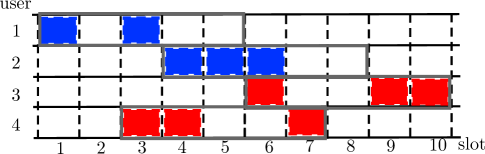
Figure 10: Frame asynchronous ALOHA with two types of heterogeneous users, where users 1 and 2 belong to the type 1 and users 3 and 4 belong to the type 2. Each user has its own view about frame of size $5$ slots, starting from the arrival of its packet.

Under the Poisson arrival process, by the superposition of independent Poisson distributions, the number of active users of type $t$, namely $K^{(t)}$, at slot $i$ again follows a Poisson distribution of rate $\mu^{(t)}_{i}$, where

$$\mu^{(t)}_{i}=\begin{cases}ig^{(t)},&\mbox{\text{for $1\leq i<N$}}\\ Ng^{(t)},&\mbox{\text{for $i\geq N$}}.\end{cases}$$ (26)

The total number of active users at slot $i$ then follows a Poisson distribution of rate $\mu_{i}=\sum_{t=1}^{T}\mu^{(t)}_{i}$.

In the presence of frame asynchrony, the proposed IRSA with NOMA protocol is modified as follows. Upon the arrival of its packet at slot $i$, a type $t$ user samples from a degree distribution $L\sim\mathcal{L}^{(t)}$ to determine the number of replicas it sends within its local view of frame. It then immediately sends one packet in slot $i$ and uniformly selects $L-1$ slots from $\mathsf{I}_{i}=[i+1:i+N-1]$ for sending the remaining $L-1$ replicas. In the decoding process, we again allow both intra-slot and inter-slot SIC, but with a sliding window fashion [52, 16]. Specifically, to decode the packets of the users joining at slot $i$, the decoder considers a sliding window of size $5N$, namely $[i:i+5N-1]$. The problem can then be treated as a realization of the frame synchronous IRSA with NOMA with frame size $5N$ and can therefore be decoded in a similar fashion.

VI-B Proposed Multi-Dimensional Density Evolution

To analyze the asymptotic performance of the proposed IRSA with NOMA in the presence of frame asynchrony, we extend the proposed multi-dimensional density evolution to the frame asynchronous setting. Here, for clearly delivering our innovation, we focus on $T=2$ again. Note that the extension to the general $T$ can be completed in the similar way to the synchronous case in Appendix A. We recall that the definitions of the node perspective degree distributions $\mathcal{L}^{(t)}[x],\mathcal{R}^{(t)}[x]$ and edge perspective degree distributions $\lambda^{(t)}[x],\rho^{(t)}[x]$ are in (5)-(7). Moreover, for a type $t$ user active at slot $i$, referred to as a class $i$ type $t$ variable node, its behavior at slot $i$ and that in slots $\mathsf{I}_{i}$ are different. We thus need to define the node perspective left degree distributions

$$\mathcal{L}^{(t)}_{i\rightarrow i}[x]=x\quad\text{and}\quad\mathcal{L}^{(t)}_{i\rightarrow\mathsf{I}_{i}}[x]=\sum_{d}L^{(t)}_{i\rightarrow\mathsf{I}_{i},d}x^{d}=\sum_{d}L^{(t)}_{d}x^{d-1},$$ (27)

where $L^{(t)}_{d,i\rightarrow\mathsf{I}_{i}}$ is the probability of a type $t$ node joining at slot $i$ that would connect with $d$ of the check nodes in $\mathsf{I}_{i}$, which is equal to $L^{(t)}_{d+1}$. As for the check nodes corresponding to slot $i$, all the edges must be incident to variable nodes with class $i$ or those with class $j\in\mathsf{K}_{i}$ where

$$\mathsf{K}_{i}=\begin{cases}\emptyset,&\mbox{\text{for $i=1$}}\\ [1:i-1],&\mbox{\text{for $2\leq i<N$}}\\ [i-N+1:i-1],&\mbox{\text{for $i\geq N$}}.\end{cases}$$ (28)

We then define the right degree distributions of a class $i$ type $t$ check node that has $d_{1}$ edges incident to class $i$ type $t$ variable nodes and that of a class $i$ type $t$ check node that has $d_{2}$ edges incident to type $t$ variable nodes in $\mathsf{K}_{i}$ as

$$\mathcal{R}^{(t)}_{i\rightarrow i}[x]=\sum_{d_{1}}R^{(t)}_{i\rightarrow i,d_{1}}x^{d_{1}}\quad\text{and}\quad\mathcal{R}^{(t)}_{i\rightarrow\mathsf{K}_{i}}[x]=\sum_{d_{2}}R^{(t)}_{i\rightarrow\mathsf{K}_{i},d_{2}}x^{d_{2}},$$ (29)

respectively.

The edge perspective degree distributions can be similarly derived as

$$\lambda^{(t)}_{i\rightarrow i}[x]=1\quad\text{and}\quad\lambda^{(t)}_{i\rightarrow\mathsf{I}_{i}}[x]=\frac{\mathcal{L}^{{}^{\prime}(t)}_{i\rightarrow\mathsf{I}_{i}}[x]}{\mathcal{L}^{{}^{\prime}(t)}_{i\rightarrow\mathsf{I}_{i}}[1]}=\sum_{d}\lambda^{(t)}_{i\rightarrow\mathsf{I}_{i},d}x^{d-2},$$ (30)

and

$$\rho^{(t)}_{i\rightarrow i}[x]=\frac{\mathcal{R}^{{}^{\prime}(t)}_{i\rightarrow i}[x]}{\mathcal{R}^{{}^{\prime}(t)}_{i\rightarrow i}[1]}=\sum_{d_{1}}\rho^{(t)}_{i\rightarrow i,d_{1}}x^{d_{1}-1}\quad\text{and}\quad\rho^{(t)}_{i\rightarrow\mathsf{K}_{i}}[x]=\frac{\mathcal{R}^{{}^{\prime}(t)}_{i\rightarrow\mathsf{K}_{i}}[x]}{\mathcal{R}^{{}^{\prime}(t)}_{i\rightarrow\mathsf{K}_{i}}[1]}=\sum_{d_{2}}\rho^{(t)}_{i\rightarrow\mathsf{K}_{i},d_{2}}x^{d_{2}-1}.$$ (31)

We note that with the proposed protocol, similar to [16, Prop. 1], we have

Proposition 11.

$$\mathcal{R}^{(t)}_{i\rightarrow i}[x]=\rho^{(t)}_{i\rightarrow i}[x]=\exp(-g^{(t)}(1-x)),$$ (32)

and

$$\mathcal{R}^{(t)}_{i\rightarrow\mathsf{K}_{i}}[x]=\rho^{(t)}_{i\rightarrow\mathsf{K}_{i}}[x]=\exp\left(-\frac{\delta^{(t)}_{i}(\mathcal{L}^{{}^{\prime}(t)}[1]-1)}{N-1}(1-x)\right),$$ (33)

where $\delta^{(t)}_{i}=\min(i-1,N-1)g^{(t)}$.

For $t\in[T]$, let $x_{{i\rightarrow i},\ell}^{(t)}$ and $x_{{i\rightarrow j},\ell}^{(t)}$ be the average erasure probability of the message passed along an edge from a class $i$ type $t$ variable node to a class $i$ type $t$ check node and that of the message passed along an edge from a class $i$ type $t$ variable node to a class $j$ type $t$ check node in iteration $\ell$, respectively. Also, we denote by $y_{{i\rightarrow i},\ell}^{(t)}$ and $y_{{i\rightarrow j},\ell}^{(t)}$ the average erasure probability of the message passed along an edge from a class $i$ type $t$ check node to a class $i$ type $t$ variable node and that of the message passed along an edge from a class $i$ type $t$ check node to a class $j$ type $t$ variable node in iteration $\ell$, respectively. In the sequel, we study how these average erasure probabilities evolve with iterations.

The average erasure probability of a message from a type $t$ check node in $\mathsf{I}_{i}$ to a class $i$ type $t$ variable node in iteration $\ell$ is given by $\tilde{y}_{i,\ell}^{(t)}=\frac{1}{N-1}\sum_{j\in\mathsf{I}_{i}}y_{{j\rightarrow i},\ell}^{(t)}.$ Then, similar to [16], we have

$$x_{{i\rightarrow i},\ell}^{(t)}=\mathcal{L}^{(t)}[\tilde{y}_{i,\ell}^{(t)}]\leavevmode\nobreak\ \quad\text{and}\quad x_{{i\rightarrow j},\ell}^{(t)}=y_{{i\rightarrow i},\ell}^{(t)}\lambda^{(t)}_{i\rightarrow\mathsf{I}_{i}}[\tilde{y}_{i,\ell}^{(t)}].$$ (34)

Also, the average erasure probability of a message from a type $t$ variable node in $\mathsf{K}_{i}$ to a class $i$ type $t$ check node in iteration $\ell$ is given by

$$\tilde{x}_{i,\ell}^{(t)}=\begin{cases}0,&\mbox{\text{for $i=1$}}\\ \frac{1}{i-1}\sum_{k\in\mathsf{K}_{i}}x_{{k\rightarrow i},\ell}^{(t)},&\mbox{\text{for $2\leq i<N$}}\\ \frac{1}{N-1}\sum_{k\in\mathsf{K}_{i}}x_{{k\rightarrow i},\ell}^{(t)},&\mbox{\text{for $i\geq N$}}.\end{cases}$$ (35)

With the above results and Proposition 11, we are now ready to present the multi-dimensional density evolution for the proposed IRSA with NOMA under the frame-asynchronous setting.

Proposition 12.

For $t\in[2]$, define

$$f_{1}(t) =\exp(-g^{(t)}x_{{i\rightarrow i},\ell}^{(t)}),$$ (36)

$$f_{2}(t) =\exp\left(-\frac{\delta_{i}^{(t)}(\mathcal{L}^{{}^{\prime}(t)}[1]-1)}{N-1}\tilde{x}_{i,\ell}^{(t)}\right),$$ (37)

$$f_{3}(t) =x_{{i\rightarrow i},\ell}^{(t)}g^{(t)}\exp(-g^{(t)}x_{{i\rightarrow i},\ell}^{(t)}),$$ (38)

$$f_{4}(t) =\tilde{x}_{i,\ell}^{(t)}\frac{\delta_{i}^{(t)}(\mathcal{L}^{{}^{\prime}(t)}[1]-1)}{N-1}\exp\left(-\frac{\delta_{i}^{(t)}(\mathcal{L}^{{}^{\prime}(t)}[1]-1)}{N-1}\tilde{x}_{i,\ell}^{(t)}\right).$$ (39)

The multi-dimensional density evolution is as follows. For $t\in[2]$, $i\in\mathbb{N}$, and $j\in\mathsf{K}_{i}$, we have

$$y_{{i\rightarrow i},\ell+1}^{(t)}=y_{{i\rightarrow j},\ell+1}^{(t)}=1-f_{1}(t)f_{2}(t)\prod_{\bar{t}\in[2],\bar{t}\neq t}\left(f_{1}(\bar{t})f_{2}(\bar{t})+f_{3}(\bar{t})f_{2}(\bar{t})+f_{1}(\bar{t})f_{4}(\bar{t})\right).$$ (40)

The proof of this result is omitted for the sake of brevity. But we point out that in (40), for $\bar{t}\neq t$, $(f_{1}(\bar{t})f_{2}(\bar{t})+f_{3}(\bar{t})f_{2}(\bar{t})+f_{1}(\bar{t})f_{4}(\bar{t}))$ corresponds to the average probability that there is at most one erasure among edges connecting to a type $\bar{t}$ check node.

VI-C Simulation Results

First, the threshold of the proposed IRSA with NOMA for the left-regular $\Lambda^{(t)}=x^{3}$ is evaluated under the frame asynchronous setting as $g=1.42$. Note that for the same left-regular degree distribution, the density evolution shows a $g=1.24$ threshold for the frame synchronous setting. This shows that, as predicted, the boundary effect helps bootstrapping the decoding process and allows the left-regular degree distribution $x^{3}$ to achieve a threshold that is close to $g=1.433$ achieved by the optimized degree distribution $\mathsf{P}_{1}$ in Table I in the frame synchronous setting. Simulation results are then provided in Fig. 11, where the packet loss rate $P_{e}$ versus sum arrival rate $g$ is plotted for $N=200$, $500$, and $1600$.

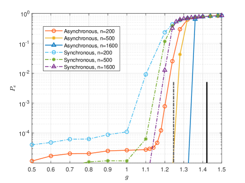
Figure 11: Packet loss rate versus sum arrival rate $g$ in the frame asynchronous setting. The thresholds obtained by the proposed density evolution are also plotted.

VII Conclusion

In this paper, we have investigated UMA in the presence of heterogeneous users. A novel protocol, IRSA with NOMA, has been proposed to leverage the heterogeneity inherent in the problem. To analyze the proposed protocol, a novel multi-dimensional density evolution has been proposed, which has been shown to be able to accurately predict the asymptotic performance of IRSA with NOMA under the modified peeling decoding. An optimization problem has then been formulated and solved for finding optimal degree distributions for our IRSA with NOMA. Simulation results have demonstrated that the proposed IRSA with NOMA can exploit the natural heterogeneity and obtained efficiency higher than that achieved by conventional IRSA. Finally, an extension of the proposed protocol to the frame-asynchronous setting has been investigated, where a boundary effect that bootstraps decoding process has been discovered via both analysis and simulation.

Throughout the paper, we have taken the MAC layer perspective. One potential future work is to extend our idea to a more practical model as in [37] and to see how randomly selecting power can further improve the performance in the presence of heterogeneity inherent in the network. Another interesting direction is to analyze how much more we can gain from having more types. From Fig. 7, we have already observed diminishing returns going from $T=2$ to $T=3$. We would expect that the $\eta^{*}$ converges to a constant as $T\rightarrow\infty$. The analysis of this convergence is left for future work.

Appendix A Multi-Dimensional Density Evolution for General $T$

In this appendix, we discuss the multi-dimensional density evolution for general $T$.

A-A Density Evolution for General $T$

For $t\in[T]$, we recall that $x_{\ell}^{(t)}$ and $y_{\ell}^{(t)}$ are the average erasure probability of the message passed along an edge from $\mathsf{v}^{(t)}$ to $\mathsf{c}^{(t)}$ and that of the message passed along an edge from $\mathsf{c}^{(t)}$ to $\mathsf{v}^{(t)}$ in iteration $\ell$, respectively. In iteration $\ell$, for an edge incident to a variable node $\mathsf{v}^{(t)}$ with degree $d$, the only possibility that the message along this edge to a $\mathsf{c}^{(t)}$ is in erasure is that all the other $d-1$ edges are in erasure. Therefore, the probability that the message passed along this edge is in erasure is $(y_{\ell}^{(t)})^{d-1}$. Now, averaging over all the edges results in the average erasure probability

$$x_{\ell}^{(t)}=\sum_{d}\lambda^{(t)}_{d}(y_{\ell}^{(t)})^{d-1}=\lambda^{(t)}[y_{\ell}^{(t)}].$$ (41)

We denote by $\mathbf{c}$ the vector whose $t$-th entry stores the number of unresolved (erased) packets. For an edge incident to a check node $\mathsf{c}^{(t)}$ with degree $d_{t}$, the message passed along this edge to a $\mathsf{v}^{(t)}$ is revealed if and only if the corresponding $\mathbf{c}$ belongs to the decodable set $\mathcal{D}^{(t)}$. Suppose in the same super check node $n$, $\mathsf{c}^{(\bar{t})}_{n}$ has degree $d_{\bar{t}}$. Then the above event has probability

$$\sum_{\mathbf{c}\in\mathcal{D}^{(t)}}(1-x_{\ell}^{(t)})^{d_{t}-c_{t}}\prod_{\bar{t}=1,\bar{t}\neq t}^{T}\binom{d_{\bar{t}}}{c_{\bar{t}}}(x_{\ell}^{(\bar{t})})^{c_{\bar{t}}}(1-x_{\ell}^{(\bar{t})})^{d_{\bar{t}}-c_{\bar{t}}}$$

$$=(1-x_{\ell}^{(t)})^{d_{t}-1}\sum_{\mathbf{c}\in\mathcal{D}^{(t)}}\prod_{\bar{t}=1,\bar{t}\neq t}^{T}\binom{d_{\bar{t}}}{c_{\bar{t}}}(x_{\ell}^{(\bar{t})})^{c_{\bar{t}}}(1-x_{\ell}^{(\bar{t})})^{d_{\bar{t}}-c_{\bar{t}}},$$ (42)

where the equality is due to the fact that every vector in $\mathcal{D}^{(t)}$ has $c_{t}=1$. Averaging over all the edges and over all the type $\bar{t}$ check nodes for $\bar{t}\in[T]\setminus\{t\}$ shows that the average probability of correct decoding is given by

$$\sum_{d_{t}}\lambda^{(t)}_{d_{t}}(1-x_{\ell}^{(t)})^{d_{t}-1}\cdot$$

$$\sum_{\mathbf{c}\in\mathcal{D}^{(t)}}\prod_{\bar{t}=1,\bar{t}\neq t}^{T}\sum_{d_{\bar{t}}}R^{(\bar{t})}_{d_{\bar{t}}}\binom{d_{\bar{t}}}{c_{\bar{t}}}(x_{\ell}^{(\bar{t})})^{c_{\bar{t}}}(1-x_{\ell}^{(\bar{t})})^{d_{\bar{t}}-c_{\bar{t}}}$$

$$=\rho^{(t)}[1-x_{\ell}^{(t)}]\sum_{\mathbf{c}\in\mathcal{D}^{(t)}}\prod_{\bar{t}=1,\bar{t}\neq t}^{T}(x_{\ell}^{(\bar{t})})^{c_{\bar{t}}}(\mathcal{R}^{(\bar{t})})^{\{c_{\bar{t}}\}}[1-x_{\ell}^{(\bar{t})}]/c_{\bar{t}}!.$$ (43)

Therefore, the average erasure probability becomes

$$y_{\ell+1}^{(t)}=1-\rho^{(t)}[1-x_{\ell}^{(t)}]\cdot$$

$$\sum_{\mathbf{c}\in\mathcal{D}^{(t)}}\prod_{\bar{t}=1,\bar{t}\neq t}^{T}(x_{\ell}^{(\bar{t})})^{c_{\bar{t}}}(\mathcal{R}^{(\bar{t})})^{\{c_{\bar{t}}\}}[1-x_{\ell}^{(\bar{t})}]/c_{\bar{t}}!.$$ (44)

Plugging (41) into (A-A) leads to the evolution of average erasure probability of a type $t$ check node as shown in (45) in the bottom of this page.

$$y_{\ell+1}^{(t)}=1-\rho^{(t)}[1-\lambda^{(t)}[y_{\ell}^{(t)}]]\cdot\sum_{\mathbf{c}\in\mathcal{D}^{(t)}}\prod_{\bar{t}=1,\bar{t}\neq t}^{T}\frac{(\lambda^{(\bar{t})}[y_{\ell}^{(\bar{t})}])^{c_{\bar{t}}}}{c_{\bar{t}}!}(\mathcal{R}^{(\bar{t})})^{\{c_{\bar{t}}\}}[1-\lambda^{(\bar{t})}[y_{\ell}^{(\bar{t})}]],\quad t\in[T].$$ (45)

A-B Convergence and Stability Condition

After obtaining the density evolution in (45), for any given degree distributions $\mathcal{L}^{(t)}$ (or $\lambda^{(t)}$) and $\mathcal{R}^{(t)}$ (or $\rho^{(t)}$), we again can analyze whether the average erasure probability converges to 0 by checking whether $y_{\ell}^{(t)}>y_{\ell+1}^{(t)}$ for every $\ell$ and every $y_{\ell}^{(t)}>0$.

In what follows, we again derive the stability condition. Similar to the $T=2$ case, we enforce $\lambda_{1}^{(t)}=0$ for all $t\in[T]$. Assuming $y^{(t)}$ is very small for all $t\in[T]$, we expand the degree distributions and approximate them by keeping only the linear terms as follows,

$$\lambda^{(t)}[y^{(t)}] \approx\lambda_{2}^{(t)}y^{(t)},$$ (46)

$$\rho^{(t)}[1-\lambda^{(t)}[y^{(t)}]] \approx 1-\rho^{{}^{\prime}{(t)}}[1]\lambda_{2}^{(t)}y^{(t)},$$ (47)

$$R^{(\bar{t})}[1-\lambda^{(\bar{t})}[y^{(\bar{t})}]] \approx 1-R^{{}^{\prime}(\bar{t})}[1]\lambda_{2}^{(\bar{t})}y^{(\bar{t})},$$ (48)

$$(R^{(\bar{t})})^{\{k\}}[1-\lambda^{(\bar{t})}[y^{(\bar{t})}]] \approx(R^{(\bar{t})})^{\{k\}}[1]$$

$$-(R^{(\bar{t})}[1])^{\{k+1\}}\lambda_{2}^{(\bar{t})}y^{(\bar{t})}.$$ (49)

We can now linearize the recursion around 0 by plugging (46)-(49) into (45) to get the same stability condition

$$\lambda_{2}^{(t)}<\frac{1}{\rho^{{}^{\prime}{(t)}}[1]}\quad\text{for $t\in[T]$}.$$ (50)

A-C Optimization Problem and Optimized Degree Distributions

Similar to the $T=2$ case, we again apply the Poisson approximation and rewrite the convergence condition in (45) as (51) in the bottom of the next page.

$$y^{(t)} > 1-\exp\left(-\eta^{(t)}\mathcal{L}^{{}^{\prime}(t)}[1]\lambda^{(t)}[y^{(t)}]\right)\cdot$$ (51)

$$\sum_{\mathbf{c}\in\mathcal{D}^{(t)}}\prod_{\bar{t}=1,\bar{t}\neq t}^{T}\frac{(\lambda^{(\bar{t})}[y_{\ell}^{(\bar{t})}]\cdot\eta^{(\bar{t})}\mathcal{L}^{{}^{\prime}(\bar{t})}[1])^{c_{\bar{t}}}}{c_{\bar{t}}!}\exp\left(-\eta^{(\bar{t})}\mathcal{L}^{{}^{\prime}(\bar{t})}[1]\lambda^{(\bar{t})}[y^{(\bar{t})}]\right),\quad t\in[T].$$

Finally, we are able to formulate the optimization problem that maximizes the target efficiency subject to derived conditions:

$$\!\max_{\{\mathcal{L}^{(t)}[x]\}} \eta=\sum_{t=1}^{T}\eta^{(t)}$$

subject to $$\text{convergence condition\leavevmode\nobreak\ }\eqref{eqn:DE_full_poisson_T},$$

$$\lambda_{1}^{(t)}=0\leavevmode\nobreak\ \text{for all $t\in[T]$},$$

$$L_{d}^{(t)}\geq 0,\leavevmode\nobreak\ \text{for all $d\in[d_{\mathrm{max}}^{(t)}]$ and $t\in[T]$},$$

$$\mathcal{L}^{(t)}[1]=1\leavevmode\nobreak\ \text{for all $t\in[T]$}.$$

Similar to $T=2$, one may include the stability condition (50) into the above optimization problem to make sure that the packet loss rate indeed vanishes as $N\rightarrow\infty$.

References

- [1] D. Evans, “The internet of things: How the next evolution of the internet is changing everything,” CISCO, White Paper, 2011.
- [2] A. Al-Fuqaha, M. Guizani, M. Mohammadi, M. Aledhari, and M. Ayyash, “Internet of things: A survey on enabling technologies, protocols, and applications,” IEEE Commun. Surv. Tutor., vol. 17, no. 4, pp. 2347–2376, Fourthquarter 2015.
- [3] 3GPP, “Feasibility study on new services and markets technology enablers,” 3rd Generation Partnership Project (3GPP), TR 22.891, Jun. 2016.
- [4] C. Bockelmann, N. K. Pratas, G. Wunder, S. Saur, M. Navarro, D. Gregoratti, G. Vivier, E. De Carvalho, Y. Ji, . Stefanović, P. Popovski, Q. Wang, M. Schellmann, E. Kosmatos, P. Demestichas, M. Raceala-Motoc, P. Jung, S. Stanczak, and A. Dekorsy, “Towards massive connectivity support for scalable mMTC communications in 5G networks,” IEEE Access, vol. 6, pp. 28 969–28 992, 2018.
- [5] D. Bertsekas and R. Gallager, Data Networks, 2nd ed. Prentice Hall, 1992.
- [6] F. Clazzer, A. Munari, G. Liva, F. Lazaro, C. Stefanovic, and P. Popovski, “From 5G to 6G: Has the Time for Modern Random Access Come?” in Proc. 1st 6G Wireless Summit, Levi, Finland, Mar. 2019.
- [7] E. Casini, R. De Gaudenzi, and O. del Rio Herrero, “Contention resolution diversity slotted ALOHA (CRDSA): An enhanced random access schemefor satellite access packet networks,” IEEE Trans. Wireless Commun., vol. 6, no. 4, pp. 1408–1419, Apr. 2007.
- [8] ETSI, “EN 301 545-2: Digital video broadcasting (DVB); second generation DVB interactive satellite system (DVB-RCS2); part 2: Lower layers for satellite standard,” Tech. Rep., 2014.
- [9] G. Liva, “Graph-based analysis and optimization of contention resolution diversity slotted ALOHA,” IEEE Trans. Commun., vol. 59, no. 2, pp. 477–487, Feb. 2011.
- [10] T. Richardsin and R. Urbanke, Modern Coding Theory. Cambridge University Press, 2008.
- [11] K. R. Narayanan and H. D. Pfister, “Iterative collision resolution for slotted ALOHA: An optimal uncoordinated transmission policy,” in Proc. ISTC, Aug 2012, pp. 136–139.
- [12] M. Luby, “LT codes,” in Proc. IEEE FOCS, Nov. 2002, pp. 271–280.
- [13] M. Luby, M. Mitzenmacher, M. A. Shokrollahi, , and D. A. Spielman, “Efficient erasure correcting codes,” IEEE Trans. Inf. Theory, vol. 47, no. 2, pp. 569–584, Feb. 2001.
- [14] G. Liva, E. Paolini, M. Lentmaier, and M. Chiani, “Spatially-coupled random access on graphs,” in Proc. IEEE ISIT, Jul. 2012.
- [15] A. Mengali, R. De Gaudenzi, and C. Stefanović, “On the modeling and performance assessment of random access with SIC,” IEEE J. Sel. Areas Commun., vol. 36, no. 2, pp. 292–303, Feb. 2018.
- [16] E. Sandgren, A. Graell i Amat, and F. Brännström, “On frame asynchronous coded slotted ALOHA: Asymptotic, finite length, and delay analysis,” IEEE Trans. Commun., vol. 65, no. 2, pp. 691–704, Feb. 2017.
- [17] S. Kudekar, T. J. Richardson, and R. L. Urbanke, “Threshold saturation via spatial coupling: Why convolutional LDPC ensembles perform so well over the BEC,” IEEE Trans. Inf. Theory, vol. 57, no. 2, pp. 803–834, Feb. 2011.
- [18] E. Paolini, G. Liva, and M. Chiani, “Coded slotted ALOHA: A graph-based method for uncoordinated multiple access,” IEEE Trans. Inf. Theory, vol. 61, no. 12, pp. 6815 – 6832, Dec. 2015.
- [19] Z. Sun, L. Yang, J. Yuan, and D. W. K. Ng, “Physical-layer network coding based decoding scheme for random access,” IEEE Veh. Technol., vol. 68, no. 4, pp. 3550–3564, Apr. 2019.
- [20] S. Zhang, S. C. Liew, and P. P. Lam, “Hot topic: Physical-layer network coding,” in Proc. ACM MobiCom, Sep. 2006, pp. 358–365.
- [21] B. Nazer and M. Gastpar, “Compute-and-forward: Harnessing interference through structured codes,” IEEE Trans. Inf. Theory, vol. 57, no. 10, pp. 6463–6486, Oct. 2011.
- [22] A. Graell i Amat and G. Liva, “Finite-length analysis of irregular repetition slotted ALOHA in the waterfall region,” IEEE Commun. Lett., vol. 22, no. 5, pp. 886–889, May 2018.
- [23] M. Ivanov, F. Brännström, A. Graell i Amat, and P. Popovski, “Error floor analysis of coded slotted ALOHA over packet erasure channels,” IEEE Commun. Lett., vol. 19, no. 3, pp. 419–422, Mar. 2015.
- [24] M. Fereydounian, X. Chen, H. Hassani, and S. S. Bidokhti, “Non-asymptotic coded slotted ALOHA,” in Proc. IEEE ISIT, Jul. 2019.
- [25] Y. Polyanskiy, “A perspective on massive random-access,” in Proc. IEEE ISIT, Jun. 2017, pp. 2523–2527.
- [26] O. Ordentlich and Y. Polyanskiy, “Low complexity schemes for the random access Gaussian channel,” in Proc. IEEE ISIT, Jun. 2017, pp. 2528–2532.
- [27] V. K. Amalladinne, J.-F. Chamberland, and K. R. Narayanan, “A coded compressed sensing scheme for unsourced multiple access,” IEEE Trans. Inf. Theory, vol. 66, no. 10, pp. 6509–6533, Oct. 2020.
- [28] A. Zaidi, F. Athley, J. Medbo, U. Gustavsson, G. Durisi, and X. Chen, 5G Physical Layer: Principles, Models and Technology Components. Academic Press, 2018.
- [29] 3GPP, “Study on Network-Assisted Interference Cancellation and Suppression (NAIC) for LTE,” 3rd Generation Partnership Project (3GPP), TR 36.866, Mar. 2014. [Online]. Available: http://www.3gpp.org/dynareport/36866.htm
- [30] G. Mazzini, “Power division multiple access,” in Proc. IEEE ICUPC’98, Oct. 1998.
- [31] L. Dai, B. Wang, Y. Yuan, S. Han, C.-L. I, , and Z. Wang, “Non-orthogonal multiple access for 5G: Solutions, challenges, opportunities, and future research trends,” IEEE Commun. Mag., vol. 53, no. 9, pp. 74–81, Sep. 2015.
- [32] Y. Saito, Y. Kishiyama, A. Benjebbour, T. Nakamura, A. Li, and K. Higuchi, “Non-orthogonal multiple access (NOMA) for cellular future radio access,” in Proc. IEEE VTC Spring, Jun. 2013, pp. 1–5.
- [33] Y. Saito, A. Benjebbour, Y. Kishiyama, and T. Nakamura, “System-level performance evaluation of downlink non-orthogonal multiple access (NOMA),” in Proc. IEEE PIMRC, Sep. 2013, pp. 611–615.
- [34] S. Ghez, S. Verdú, and S. Schwartz, “Stablity properties of slotted ALOHA with multipacket reception capability,” IEEE Trans. Autom. Control, vol. 33, no. 7, pp. 640–649, Jul. 1988.
- [35] M. Ghanbarinejad and C. Schlegel, “Irregular repetition slotted ALOHA with multiuser detection,” in 2013 10th Annual Conference on Wireless On-demand Network Systems and Services (WONS), Mar. 2013.
- [36] C. Stefanović, E. Paolini, and G. Liva, “Asymptotic performance of coded slotted ALOHA with multipacket reception,” IEEE Commun. Lett., vol. 22, no. 1, pp. 105–108, Jan. 2018.
- [37] A. Mengali, R. Gaudenzi, and P.-D. Arapoglou, “Enhancing the physical layer of contention resolution diversity slotted ALOHA,” IEEE Trans. Commun., vol. 65, no. 10, pp. 4295–4308, Oct. 2017.
- [38] A. Benjebbour, Y. Kishiyama, and Y. Okumura, “Special articles on 5G standardization trends toward 2020: Field trials of improving spectral efficiency by using a smartphone-sized NOMA chipset,” NTT DOCOMO Technical Journal, vol. 20, no. 1, pp. 4–13, Jul. 2018.
- [39] T. M. Cover and J. A. Thomas, Elements of Information Theory. Wiley, 1991.
- [40] A. Yedla, P. S. Nguyen, H. D. Pfister, and K. R. Narayanan, “Universal codes for the Gaussian MAC via spatial coupling,” in Proc. Allerton Conf., Sep. 2011.
- [41] J. Zhu and M. Gastpar, “Gaussian multiple access vai compute-and-forward,” IEEE Trans. Inf. Theory, vol. 63, no. 5, pp. 2678–2695, May 2017.
- [42] U. Erez and R. Zamir, “Achieving on the AWGN channel with lattice encoding and decoding,” IEEE Trans. Inf. Theory, vol. 50, no. 10, pp. 2293–2314, Oct. 2004.
- [43] J. Choi, “NOMA-based random access with multichannel ALOHA,” IEEE J. Sel. Areas Commun., vol. 35, no. 12, pp. 2736–2743, Dec. 2017.
- [44] ——, “Multichannel NOMA-ALOHA game with fading,” IEEE Trans. Commun., vol. 66, no. 10, pp. 4997–5007, Oct. 2018.
- [45] F. Clazzer, E. Paolini, I. Mambelli, and C. Stefanović, “Irregular repetition slotted ALOHA over the Rayleigh block fading channel with capture,” in Proc. IEEE ICC, May 2017.
- [46] T. Polonelli, D. Brunelli, and L. Benini, “Slotted aloha overlay on LoRaWAN - a distributed synchronization approach,” in IEEE 16th International Conference on Embedded and Ubiquitous Computing, Oct. 2018.
- [47] 3GPP, “Solutions for nr to support non-terrestrial networks (NTN),” 3rd Generation Partnership Project (3GPP), TR 38.821, Aug. 2018.
- [48] B. S. Tsybakov and V. A. Mikhailov, “Ergodicity of a slotted ALOHA system,” Problemy Peredachi Informatsii, vol. 15, no. 4, pp. 73–87, 1979.
- [49] M. Mitzenmacher and E. Upfal, Probability and Computing: Randomized Algorithms and Probabilistic Analysis. Cambridge University Press, NY, USA, 2005.
- [50] K. Price, R. M. Storn, and J. A. Lampinen, Differential Evolution: A Practical Approach to Global Optimization. Springer, 2005.
- [51] Y. Li, Z. Zhan, Y. Gong, W. Chen, J. Zhang, and Y. Li, “Differential evolution with an evolution path: A DEEP evolutionary algorithm,” IEEE Trans. Cybern., vol. 45, no. 9, pp. 1798–1810, Sep. 2015.
- [52] A. Meloni, M. Murroni, C. Kissling, and M. Berioli, “Sliding window-based contention resolution diversity slotted ALOHA,” in Proc. IEEE Globecom, Dec. 2012, pp. 3305–3310.