Binding and Perspective Taking as Inference
in a Generative Neural Network Model

Abstract

The ability to flexibly bind features into coherent wholes from different perspectives is a hallmark of cognition and intelligence. Importantly, the binding problem is not only relevant for vision but also for general intelligence, sensorimotor integration, event processing, and language. Various artificial neural network models have tackled this problem with dynamic neural fields and related approaches. Here we focus on a generative encoder-decoder architecture that adapts its perspective and binds features by means of retrospective inference. We first train a model to learn sufficiently accurate generative models of dynamic biological motion or other harmonic motion patterns, such as a pendulum. We then scramble the input to a certain extent, possibly vary the perspective onto it, and propagate the prediction error back onto a binding matrix, that is, hidden neural states that determine feature binding. Moreover, we propagate the error further back onto perspective taking neurons, which rotate and translate the input features onto a known frame of reference. Evaluations show that the resulting gradient-based inference process solves the perspective taking and binding problem for known biological motion patterns, essentially yielding a Gestalt perception mechanism. In addition, redundant feature properties and population encodings are shown to be highly useful. While we evaluate the algorithm on biological motion patterns, the principled approach should be applicable to binding and Gestalt perception problems in other domains.

Introduction

Social cognition depends on our ability to understand the actions of others. The simulation theory of social cognition (Barsalou 1999; Gallese and Goldman 1998; Johnson and Demiris 2005) suggests that visual and other sensory dynamics are mapped onto the own sensorimotor system. The mirror neuron system has been proposed to play a fundamental role in this respect. It appears to project and interpret visual information about others with the help of ones own motor repertoire (Gallese, Keysers, and Rizzolatti 2004). Cook et al. (2014) argue that the involved mirror neurons can develop purely via associative learning mechanisms. Two fundamental challenges remain, however, when attempting to learn such associations: the perspective taking problem and the binding problem.

The perspective taking problem addresses the challenge that visual information about others comes in a different frame of reference than information about ones own body. It has been shown that we have a strong tendency to adapt the perspective of others, particularly when observing interactions with other entities (Tversky and Hard 2009). These and related results and modeling work suggest that our brain is able to project our own perspective into the other person by some form of transformation (Johnson and Demiris 2005; Meltzoff and Prinz 2002; Schrodt et al. 2014). Indeed, in adults this ability it not restricted to spatial transformations but extends to the adoption of, for example, conceptual and affective standpoints (Moll and Meltzoff 2011). When focusing on spatial perspective taking, the challenge is to transform an observed action into a canonical perspective, to thus prime corresponding motor simulations (Castiello et al. 2002; Edwards, Humphreys, and Castiello 2003).

Besides the perspective taking challenge, the binding problem (Butz and Kutter 2017; Treisman 1998) poses another severe challenge. In particular, individual visual features, such as motion patterns, color, texture, or edge detectors, have to be integrated into a complete Gestalt (Jäkel et al. 2016; Koffka 2013) in order to recognize an entity, such as the body of another person. With respect to biological motion recognition, the problem has also been termed the correspondence problem (Nehaniv, Dautenhahn et al. 2002; Heyes 2001): Which observed body part corresponds to which own body part? Action understanding and imitation appears to be facilitated by establishing correspondences between the own body schema and the one of an observed person (Jackson, Meltzoff, and Decety 2006). To bind the observed features together into an integrated bodily percept, top-down expectations are interacting with bottom-up saliency cues in an approximate Bayesian manner (Buschman and Miller 2007; Jäkel et al. 2016). The details of the involved processes, however, remain elusive.

Here we propose a generative, autoencoder-based neural network model, which solves the perspective taking and binding problems concurrently by means of retrospective, prediction error-minimizing inference. The encoder part of the model is endowed with a transition vector and a rotation matrix for perspective taking and a binding matrix for flexibly integrating input features into one Gestalt percept. The parameters of these three modules are tuned online by means of retrospective inference (Butz et al. 2019). As a result, the model mimics approximate top-down inference, attempting to integrate all bottom-up visual cues into a Gestalt from a canonical perspective. The model is first trained on a canonical perspective of an ordered set of motion features, simulating a self-grounded Gestalt perception (Gallese, Keysers, and Rizzolatti 2004). Next, perspective taking and feature binding is evaluated by projecting the reconstruction error back onto the perspective and binding parameters, which can be viewed as specialized parametric bias neurons (Sugita, Tani, and Butz 2011; Tani 2017). Our evaluations show that it is highly useful (i) to split the motion feature information into relative position, motion direction, and motion magnitudes and (ii) to use population encodings of the individual features. We evaluate the model’s abilities on a two dimensional, two joint pendulum and on three dimensional cyclic dynamical motion patterns of a walking person.

Proposed Model

The proposed architecture has some fixed components and some other components that are trained or adapted online by backpropagation. The model learns a generative, autoencoder-based model of motion patterns, which it employs to bind visual features and perform spatial perspective taking. In our case, each visual feature corresponds to a joint location and is represented by a Cartesian coordinate relative to a global six-dimensional frame of reference (encoding origin and orientation). Figure 1 shows a sketch of the processing and inference architecture.

Sub-Modal Population Encoding

Each Cartesian input coordinate at each time step $t$ is segregated into three distinct sub-modalities (i.e. posture, motion direction, and motion magnitude). Note that the relative position of a visual feature depends on the choice of origin and the orientation of the coordinate frame. Moreover, while motion direction depends only on the orientation but not on the origin, motion magnitude is completely independent of perspective. As a result, given a visual input coordinate and its velocity, three types of submodal information are derived each transformed via a rotation matrix $R$ and a translation bias $b$, which determine orientation and origin, that is, the frame of reference, respectively. At each point in time $t$, the transformations are applied as follows:

$$P_{i}(t)=R(t)\cdot X_{i}(t)+b(t),$$ (1)

determining the relative position $P_{i}(t)$ of the feature $X_{i}(t)$;

$$m_{i}(t)=\left\|R(t)\cdot V_{i}(t)\right\|,$$ (2)

where $V_{t}=X_{t}-X_{t-1}$ denotes the velocity to determine the absolute motion magnitude $m_{i}(t)$;

$$d_{i}(t)=\frac{R(t)\cdot V_{i}(t)}{m_{i}(t)},$$ (3)

calculating the relative motion direction $d_{i}(t)$. Figure 1 shows a sketch of the proposed model in a connectivity graph, including the processing pipeline for a single three dimensional visual feature.

Figure 1: Our generative, modularized neural network model processes a visual feature $i$ by first applying possible translation and rotation operations. Next, the feature is encoded into respective population codes. A neural gating matrix binds feature $i$ to an autoencoder input slot $j$. Variational autoencoders for posture, motion direction, and magnitude attempt to reconstruct the observed patterns. The squared difference between input and reconstruction is used as the loss signal to adjust the parameters of the gating and rotation matrices and the translation vector via retrospective inference.

After the extraction of submodal information and the projection onto a particular visual frame of reference, each submodality is encoded separately by one population of topological neurons with Gaussian tunings, which yield local responses to specific stimuli within a limited range. Such encodings can be closely related to encodings found in the visual cortex and beyond (Olshausen and Field 1997; Pouget, Dayan, and Zemel 2000). However, to assess the effectiveness of population coding, we also evaluate the model’s performance on the raw submodal information. The topological neurons of posture, direction, and magnitude populations are evenly projected onto a cube, a unit sphere, and a line, respectively, such that the input space is fully covered. According to the motion capture data and the applied skeleton, posture, direction, and magnitude populations are configured to contain $64$, $32$, and $4$ neurons, respectively. In the case of the two jointed pendulum experiments, we distributed $16$ posture neurons on a rectangle area around the stimuli, $8$ direction neurons on a unique circle, and $4$ magnitude neurons. The response $\smash{\dot{P}_{\alpha i}}$ of the $\alpha$-th neuron in a population that encodes the position $p$ of the i-th visually observed feature is computed by:

$$\dot{P}_{\alpha,i}(t)=(r^{p})^{D^{p}}\cdot N\left(P_{i}(t);c_{\alpha}^{p},\Sigma^{p}\right)$$ (4)

where $N(l;\mu,\Sigma)$ is the density of the multivariate normal distribution at $l$ with mean $\mu$ and a $D^{p}$-dimensional diagonal covariance matrix $\Sigma$. Each neuron in a submodal feature population has an individual center $c_{\alpha}^{p}$ as well as a response variance $\Sigma^{p}$. The factor $\smash{(r^{p})^{D^{p}}}$ scales the neural activities, dependent on the relative distance $r^{p}$ between neighboring neurons. The individual neuron centers are evenly distributed in the expected range of the submodal stimuli. The relative distance $r^{p}$ is also used to determine the diagonal variance entries:

$$\sigma^{p}=\zeta^{p}\cdot(r^{p})^{2},$$ (5)

where $\zeta^{p}\in(0,1]$ modulates the breadth of the cell tunings. Similarly, topological neurons’ activations for direction and magnitude sub-modalities are computed by:

$$\dot{d}_{\alpha,i}(t)=(r^{d})^{D^{d}}\cdot N\left(d_{i}(t);c_{\alpha}^{d},\Sigma^{d}\right),$$ (6)

$$\dot{m}_{\alpha,i}(t)=(r^{m})^{D^{m}}\cdot N\left(m_{i}(t);c_{\alpha}^{m},\Sigma^{m}\right),$$ (7)

where the centers are set up to be in accordance with the dimension, range, and configuration space of the respective submodal stimuli. Consequently, neurons that encode visual positional features ($D^{p}=3$; $2$ for pendulum) are arranged evenly on a grid in a specific range. Neurons that encode visual directional motion are arranged on the surface of a unit sphere ($D^{d}$ = 3; 2 for pendulum), while neurons that encode visual motion magnitudes are distributed linearly ($D^{m}$ = 1). Resulting population encoding activities are shown exemplarily in Figure 1.

Gestalt Perception and Feature Binding

The binding problem concerns the selection and integration of separate visual features in the correct combination (Treisman 1998). An approach for solving this problem is to selectively route respective feature positions and motion dynamics such that the rerouted feature patterns match expected Gestalt dynamics.

Both the selection of features relevant for the recognition of biological motion and the assignment to the respective neural processing pathways are handled by an adaptive, gated connectivity matrix, which routes observed features $i\in\left\{1...N\right\}$ to bodily features $j\in\left\{1...M\right\}$ as follows:

$$\ddot{p_{j}}(t)=\sum_{i=1}^{N}w_{ij}(t)\cdot\dot{p_{i}}(t),$$ (8)

$$\ddot{d_{j}}(t)=\sum_{i=1}^{N}w_{ij}(t)\cdot\dot{d_{i}}(t),$$ (9)

$$\ddot{m_{j}}(t)=\sum_{i=1}^{N}w_{ij}(t)\cdot\dot{m_{i}}(t),$$ (10)

where $\ddot{p_{j}}$, $\smash{\ddot{d_{j}}}$, and $\ddot{m_{j}}$ represent the population encoded activations of the j-th assigned or bodily submodal feature in the position, motion direction, and motion magnitude domains, respectively. $\dot{p_{j}}$, $\smash{\dot{d_{j}}}$, and $\dot{m_{j}}$ represent the according activity of the i-th unassigned or observed submodal feature, and $w_{ij}\in(0,1)$ represents the corresponding assignment strength. The assignment strength is implemented by a non-linear neuron with logistic activation function:

$$w_{ij}=\frac{1}{1+exp(-w_{ij}^{b})}$$ (11)

where $w_{ij}^{b}$ denotes the activity of an adaptive parametric bias neuron. Each set of submodal bodily feature populations is joined into a submodal Gestalt vector $g^{x}$:.

$$g^{p}(t)=(\ddot{p}_{1}(t),\ddot{p}_{2}(t),...,\ddot{p}_{M}(t)),$$ (12)

$$g^{d}(t)=(\ddot{d}_{1}(t),\ddot{d}_{2}(t),...,\ddot{d}_{M}(t)),$$ (13)

$$g^{m}(t)=(\ddot{m}_{1}(t),\ddot{m}_{2}(t),...,\ddot{m}_{M}(t)),$$ (14)

yielding Gestalt vectors for the posture, motion direction, and motion magnitude submodalities, respectively.

To learn distributed, predictive encodings of actions, each submodal Gestalt perception $x\in\{p,d,m\}$ is encoded by one variational autoencoder (VAE, Kingma and Welling 2013). The bottom-up activated submodal Gestalt vectors $g^{x}$ are thus passed through the autoencoder, generating reconstructions of the Gestalt perceptions. As a consequence, when a fully trained autoencoder is provided with an imperfect stimulus (e.g. an observed action with unknown identity of the features, shown from an unknown perspective), it will tend to infer the closest known stimulus pattern, which will correspond to its (simulated) embodied, or self-perceptual experience. The respective autoencoders thus generate posture, motion direction, and magnitude predictions. After model learning, the difference between the Gestalten input to the autoencoder and the regenerated Gestalten output is to be minimized by adapting the parametric bias neurons’ activities of the binding matrix and the perspective taking modules. We denote the respective squared losses by $\mathcal{L}(p)$, $\mathcal{L}(d)$, and $\mathcal{L}(m)$, respectively. We scale the loss signals by respective factors $\beta^{p}$, $\beta^{d}$, and $\beta^{m}$ to balance the error signal influences. The actual adaptation of the parametric bias neurons’ activities $w_{ij}^{b}(t)$ is computed by typical gradient descent with momentum:

$$\Delta w_{ij}^{b}(t)=~{}-\eta^{f}\frac{\partial\mathcal{L}(t)}{\partial w_{ij}^{b}(t)}+\gamma^{f}(w_{ij}^{b}(t-1)-w_{ij}^{b}(t-2)),$$ (15)

where $\gamma^{f}$ denotes the momentum, $\eta^{f}$ the learning rate for the feature binding adaptation process, and the loss signal $\mathcal{L}(t)$ equals to:

$$\mathcal{L}(t)=\beta^{p}\mathcal{L}_{p}(t)+\beta^{d}\mathcal{L}_{d}(t)+\beta^{m}\mathcal{L}_{m}(t)$$ (16)

During training, the assignment biases $w_{ij}^{b}$ are fixed to $w_{ii}=1000$ for all $i$ (resulting in $w_{ii}\approx 1$) and to $w_{ij}=-1000$ for all $i\neq j$ (resulting in $w_{ij}\approx 0$), because the assignment is fixed during simulated self-observations. During testing, all assignment biases are initialized to $-1$, resulting in an initial subtle mixture of all possible assignments, and are adapted over time by means of Eq 15.

Perspective Taking

Perspective taking consists of a translation followed by a rotation of all considered visual features. The employed mechanism is based on (Schrodt et al. 2015). It aims at establishing the best possible correspondence between the input and top-down expectations. The translation determines the origin of the model’s internal, imagined frame of reference as well as the center of rotation. Perspective taking can be thought of as a mental transformation process that aligns the observer’s perspective with a canonical, self-centered perspective. The translation is determined by the bias neurons $b_{a}$, which, again, are adapted by gradient descent with momentum to minimize the top-down loss signal $\mathcal{L}(t)$:

$$\Delta b_{a}(t)=~{}-\eta^{b}\frac{\partial\mathcal{L}(t)}{\partial^{t}b_{a}(t)}+\gamma^{b}(b_{a}(t-1)-b_{a}(t-2))$$ (17)

where $a\in\left\{x,y,z\right\}$ denotes the affected axis, $\gamma^{b}$ the momentum term, and $\eta^{b}$ the adaptation rate. The translation biases $b_{a}$ are initialized to 0. Note that motion direction and magnitude are invariant to translations. As a result, the adaptation is determined the posture-respective weighted error signals $\beta^{p}\Delta_{1...M}^{p}$ only (cf. also Figure 1).

Rotation is performed via a neural $3\times 3$ matrix $R$, which is driven by three Euler angles $\alpha_{x}$, $\alpha_{y}$ , and $\alpha_{z}$ each of which represents rotation around a specific Cartesian axis. The corresponding pre-synaptic connection structure is shown in the following equation:

$$R=R_{x}(\alpha_{x}(t))R_{y}(\alpha_{y}(t))R_{z}(\alpha_{z}(t))$$ (18)

Similar to the translation, the rotation is represented by bias neurons, which can be adapted online by gradient descent. The adaptation over time follows the rule

$$\Delta\alpha_{a}(t)=~{}-\eta^{r}\frac{\mathcal{L}(t)}{\partial^{r}\alpha_{a}(t)}+\gamma^{r}(\alpha_{a}(t-1)-\alpha_{a}(t-2))\\$$ (19)

where $a\in\left\{x,y,z\right\}$, $\gamma^{r}$ specifies the momentum, and $\eta^{r}$ the adaptation rate. Note that motion magnitude is invariant to rotation by nature and thus not considered in this process. The rotation biases are initialized to 0.

Related Work

From the brain-inspired side, dynamic neural fields are principally closely related to our model (Erlhagen and Schöner 2002; Erlhagen and Bicho 2006) in that the activities in multiple dynamic neural fields strive for an overall consistent encoding. For example, they dynamically develop mappings between spatial task parameters that can resolve redundancies while generating motor plans (Erlhagen and Schöner 2002; Martin, Reimann, and Schöner 2019; Martin, Scholz, and Schöner 2009). More generally, it has been recently shown that dynamic neural fields can establish temporal bindings between different conceptual representations such as spatial arrangements of objects and compatible linguistic descriptions thereof (Sabinasz et al. 2020; Schöner 2019). Our perspective taking mechanisms can also be loosely related to neurocomputational models, which approximate actual representation formats identified in the brain (Denève and Pouget 2004; Pouget, Dayan, and Zemel 2000, 2003).

From the deep learning side, transformer networks (Jaderberg et al. 2015) are rather closely related in that an affine transformation is proposed, which works similar to our perspective taking module. In contrast to our work, though, the transformer network infers the frame of reference purely stimulus driven in a feed-forward manner. Our model couples the perspective taking module with a generative model, enabling retrospective inference of the perspective taking parameters. Moreover, various attentional mechanisms can be considered related (Vaswani et al. 2017) seeing that these architectures selectively process information. In contrast, our binding matrix flexibly reroutes information in the attempt to bind the information retrospectively rather than in a feed-forward manner, which may be more closely related to capsule networks (Sabour, Frosst, and Hinton 2017). Our binding matrix adaptation mechanism may be most closely related to Memisevic (2013), where gated autoencoder (or restricted Boltzmann machine) structures are learned. In our case, we apply the binding matrix, which is similar to gating, before the actual autoencoding.

Experimental Results

We evaluate our model on a simple two-joint pendulum task as well as on more challenging 3D bodily motion capture data. For the latter, we use the Motion Capture (MoCap) database of the Graphics Lab of the Carnegie Mellon University (CMU 2018). The CMU motion tracking data was recorded with $12$ high-resolution infrared cameras, each of which was recording at $120$Hz using $41$ tracking markers taped on jumpsuits of human subjects. Every marker provided a 3D bodily landmark position, which was then mapped onto a skeleton file, which specifies limb connectivities and lengths. Here we focus on continuous, cyclic actions and therefore use the motion capture data specified in Table 1, which offers cyclic 3D walking motion patterns of three different participants. Out of $30$ limbs provided by the skeleton file, $M=$ 15 were selected as visual inputs, as shown in Figure 2 left. To generate clean training data , we extracted a short episode of a walking trial of 260 time steps of Subject 35 and manually edited it to form a continuous cycle with 1036 frames in total. We edited walking trials of Participants 5 and 6 in a similar manner, yielding 1000 frames in total, each.

Table 1: Used data for training and testing the model

	Training	Testing
3D Walking	Subject 35, 7 cycles, 1036 frames	Subjects 5 and 6,  7 cycles, 1000 frames
2D Pendulum	6 cycles, 1000 frames	same pattern

As another generic case we trained the model with generated two jointed pendulum data, which we adapted from mathplotlib’s animation example (Pen 2017). It consist of 0.8 and 0.6 meter length plus 1.25 and 1 kilogram mass of the corresponding joints 1 and 2. The data used for training and testing at the pendulum swing back and forth seven times with completely loose lower limb.

If not stated differently, all results reported below show averages (and standard deviations where possible) over ten independently trained networks.

VAE Prediction Error

During training the model has full access to visual information and visual stimuli are perceived from an egocentric point of view (perspective taking and feature binding adaptations are disabled). The aim is to analyze the compression quality of the autoencoder. We used the PyTorch library of Python. The chosen network parameters are specified in Table 2. Grid search was used to determine good parameter settings. While a more detailed analysis of parameter influences is beyond the scope of this paper, we can state that medium parameter value variations did not appear to change the reported results in any fundamental manner. To evaluate the influence of population coding on the model, we also trained another VAE model without the population encoding, feeding the raw Cartesian data into the VAE. In both cases, the model was able to significantly improve its reconstruction error over time, as can be clearly seen in Figure 2 right. Albeit the different error measures without and with population encoding cannot be directly compared, it is well-noticeable that learning takes place in both cases. Moreover, the relative improvement particularly of posture and motion direction Gestalt reconstruction error is much stronger in the case of population encoding (note the different ranges of the y-axes).

Table 2: Used data for training the variational autoencoder

Experiment	Learning Rate Pos	Learning Rate Dir	Learning Rate Mag	Optimization	Hidden Size	Latent Size	$\zeta^{p}$	$\zeta^{d}$	$\zeta^{m}$
Using population coding	$1\cdot 10^{-3}$	$8\cdot 10^{-4}$	$5\cdot 10^{-4}$	Adam	45	25	0.85	0.85	0.95
Using raw data	$1\cdot 10^{-3}$	$2\cdot 10^{-5}$	$8\cdot 10^{-4}$	Adam	25	10	-	-	-
Two Jointed Pendulum	$1\cdot 10^{-2}$	$1\cdot 10^{-2}$	$1\cdot 10^{-3}$	Adam	45	25	0.85	0.85	0.95

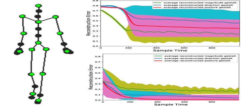
Figure 2: left: Motion capture skeleton data indicating the chosen 15 features; right: Visual spatial reconstruction error (i.e. Binary Cross-Entropy Loss) of posture, direction, and magnitude Gestalt perceptions; right-up: trained when using no population coding; right-down:trained using population coding

Adaptation of Feature Binding

While the results above show that the VAE does learn good encodings, the critical question in this work was whether the resulting signal is useful to accomplish feature binding and perspective taking, which we evaluate separately. To focus on feature binding, we disabled perspective taking. Neural feature binding bias activities $w_{ij}^{b}$ were reset to $-5$ for each test trial, resulting in assignment strengths of $w_{ij}\approx 0.0067$ effectively distributing all feature value information uniformly over the VAE inputs. Please note that it is not necessary to permute the order of the inputs for the evaluation, since the model loses its knowledge about the correct assignment at this point. The hyperparameters used during the feature binding experiments are shown in Table 3.

Table 3: Hyperparameters used for feature binding

Experiment 1	Experiment 2	Experiment 3	Experiment 4
No Pop Code	With Pop Code	With Pop Code	2D Pendulum
$\beta^{pos}$= 5	$\beta^{pos}$= 6	$\beta^{pos}$= 8	$\beta^{pos}$= 1
$\beta^{dir}$= 1	$\beta^{dir}$= 0	$\beta^{dir}$= 2	$\beta^{dir}$= 8
$\beta^{mag}$= 0.125	$\beta^{mag}$= 0	$\beta^{mag}$= 0.125	$\beta^{mag}$= 2
$\eta^{f}$= 1	$\eta^{f}$= 1	$\eta^{f}$= 1	$\eta^{f}$= 0.1
$\gamma^{f}$= 0.9	$\gamma^{f}$= 0.9	$\gamma^{f}$= 0.9	$\gamma^{f}$= 0.9

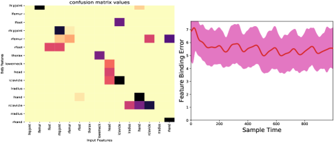
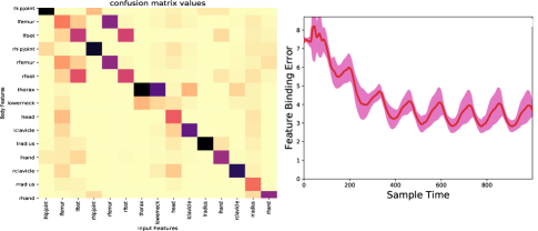
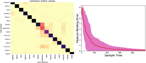
Figure 3: Adapting the feature binding at first three experiments mentioned in Table 3

To measure the progress of feature binding in these experiments, we define a Feature Binding Error (FBE) as the sum of Euclidean distances between the model’s assignment of a bodily feature and the correct assignment:

$$FBE(t)=\sum_{j=1}^{M}\sqrt{(w_{jj}(t)-1)^{2}+\sum_{i=1,i\neq j}^{N}w_{ii}(t)^{2}}$$ (20)

Figure 4 shows that the feature binding error decreases in all encoding cases. Moreover, Figure 3 shows the resulting binding matrix values after 1000 steps of feature binding adaptation. Clearly, the applied population encoding is highly useful to decrease the FBE and thus to identify the right feature bindings, which corresponds to the diagonal. Please note again that the diagonal is identified without prior assumptions, that is, any other feature shuffling will yield the same result. It is interesting to analyze the binding matrix values, which essentially can be interpreted as a confusion matrix, in further detail. Without population encoding, full binding matrix convergence does not take place. For example, the hip joint is confused with the femur, and even severe confusions can be observed, such as the left foot with the left clavicle.

With population encoding, the FBE drops significantly lower. When only the posture encoding is considered, however, left-right and neighboring limb confusions remain. Only when motion information is added in population encoded form, hardly any confusions remain, indicating full Gestalt perception. It may be noted that the probability to guess the correct assignment by chance is virtually impossible (225 choose 15 yields a value of $9.1\cdot 10^{22}$ possibilities). The results clearly show that the VAE is able to identify the right bindings, particularly when population encodings are used and complementary feature information is provided. It is noticeable that the population encodings essentially enable the encoding of multi-modal distributions, which may be highly useful to test multiple binding options concurrently, most effectively guiding the binding values to the most consistent overall assignment over time. Additionally, the complementary information from posture, motion direction, and motion magnitude help to resolve remaining ambiguities.

To verify the generality of our results, we also evaluated binding performance on the pendulum data. Figure 4 confirms that binding also works robustly for the two joint pendulum data. Even if some latent activity of Joint 2 is added to Joint 1, this disruption seems to be minor, also indicating robust Gestalt perception.

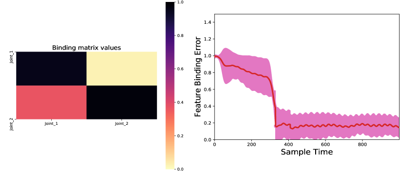
Figure 4: Adapting the feature binding on two jointed pendulum

Adaptation of Perspective Taking

Focusing on perspective taking next, we fix the binding matrix to the correct diagonal binding values and assess the complexity when facing different perspectives onto a known motion pattern. Thus, we confront the fully trained models with trials of the test set, fix the binding matrix, and evaluate the development of spatial translation and orientation parametric biases. Each motion capture trial is first transformed by a random, three-dimensional, constant rotation offset, followed by a translation offset, before feeding it into the the model. As a result, the model perceives the data from an unknown viewpoint and needs to transfer it into its known, egocentric frame of reference. As a quantitative measure for the transformation progress, we define an orientation difference (OD) measure:

$$OD(t)=\frac{180}{2\Pi}Acos(\frac{tr(A^{model}(t)A^{data}(t))-1}{2})\text{in}\,^{\circ},$$ (21)

where $A^{data}$ is a constant rotation matrix applied to all visual inputs and $A^{model}$ is the dynamic, currently inferred rotation matrix of the model. For measuring the translation with respect to the learned egocentric view, a translation difference (TD) measure is used:

$$TD(t)=\left\|b^{data}(t)-b^{model}(t)\right\|\text{in cm},$$ (22)

where $b^{data}$ is the constant per trial offset applied to the data and $b^{model}$ is the momentary adaptation of the model. Employed model parameters are shown in Table 4.

Table 4: Hyperparameters used for perspective taking

Parameter	$\eta^{r}$	$\gamma^{r}$	$\eta^{b}$	$\gamma^{b}$	$\beta^{pos}$	$\beta^{dir}$	$\beta^{mag}$
Value	$1.10^{-2}$	$9.10^{-1}$	$8.10^{-2}$	$9.10^{-1}$	8	3	0.125

Figure 6 shows the trained Rotation matrix while all visual input data was rotated with randomly assigned $\alpha_{x}$, $\alpha_{y}$ and $\alpha_{z}$ for one of the trained networks (results were qualitatively equivalent for the other trained networks). Figure 6 shows the corresponding translation bias inference during testing for the same network. As can be seen, the stronger the perspective is disturbed, the longer it takes to infer the correct perspective. Rather extreme rotations of close to $90^{\circ}$ on all three axes are hardest. Similarly, strong translations yield delayed convergence, as can be expected.

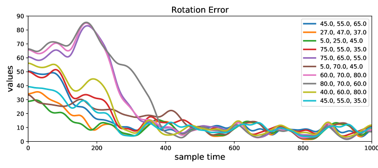
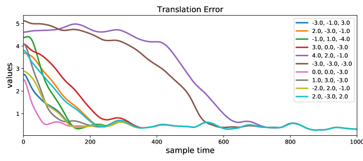
Figure 5: Adapting the Perspective Taking: Rotation

Figure 6: Adapting the Perspective Taking: Translation

To explore the perspective taking abilities further, we exemplarily look at the performance of a case where both rotations and translations are applied to the input data (we set $b_{x}=-2$ , $b_{y}=2.5$, $b_{z}=-4$, $R_{x}=25^{\circ}$ , $R_{y}=35^{\circ}$, $R_{z}=45^{\circ}$). Figure 7 shows that also in the case of perspective taking the population encoding is highly useful. Moreover, it confirms that translation and rotation distortions can be optimized concurrently.

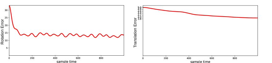
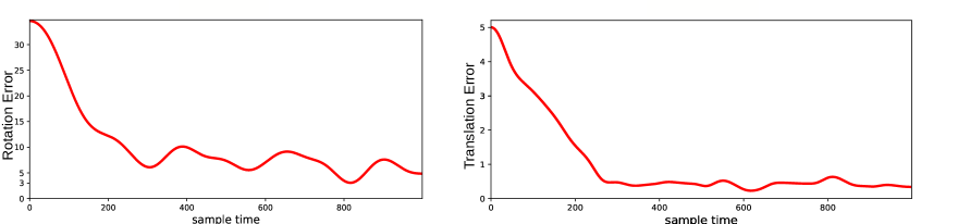
Figure 7: Adapting rotation and translation; Upper-Row: no population coding; Lower-Row: With population coding

Summary and Conclusion

We have introduce a generative neural network architecture, which tackles the perspective taking and binding challenges. In contrast to related approaches, such as attention-based architectures (Vaswani et al. 2017) or transformer networks (Jaderberg et al. 2015), our system applies retrospective inference tuning parametric bias neurons (Sugita, Tani, and Butz 2011; Tani, Ito, and Sugita 2004; Tani 2017), which are in our case dedicated to establish feature bindings and adapt the internal perspective onto the observed features. The flexible binding is most closely related to tripartite autoencoder and Restricted Boltzmann machine approaches (Memisevic 2013) as well as to capsule networks (Sabour, Frosst, and Hinton 2017). In contrast, our model applies a more direct, retrospective gradient-based adaptation mechanism to latent, dedicated parametric bias neurons, adhering to the principle of endowing neural network architectures with effective inductive learning and inference biases (Battaglia et al. 2018). As a result, starting from a canonical perspective on a biological motion pattern, we have shown that perspective taking and binding works highly reliably, particularly when complementary spatio-temporal feature patterns are available and encoded with population codes. Interestingly, the resulting ability can be related to embodied social cognition, mirror neurons, perspective taking, and Gestalt perception.

Despite the success in both feature binding and perspective taking online, future work is necessary to investigate scalability and robustness of our model. In order to be able to distinguish multiple Gestalt patterns, another top-down module needs to be added, which may be able to identify distinct motion patterns, such a walking, running, jumping, but also static patterns, such as sitting, standing, or lying down (cf. Butz et al. 2019; Schrodt and Butz 2016; (Schrodt 2018). Moreover, we intend to extend the model with an LSTM-based temporal encoder-decoder architecture (Bahdanau, Cho, and Bengio 2015), in order to reap additional information from the temporal dynamics retrospectively (Butz et al. 2019). Seeing that we did not need to add any regularization methods, residual connections, or other techniques useful for scaling-up deep ANN (Goodfellow, Bengio, and Courville 2016), we are confident that our approach will be applicable to larger dataset and disjunct Gestalt patterns.

Overall, we hope that our technique will be useful also in other domains, where information needs to be flexibly bound together and associated to other data on the fly, striving for overall consistency. Seeing that perspective taking and binding problems are universal problems in cognitive science, the proposed architecture and retrospective inference mechanisms may be very useful also in solving related challenges in other domains besides biological motion patterns.

References

- Pen (2017) 2017. Mathplotlib animation Examples; double pendulum Release: 2.0.2. https://matplotlib.org/examples/animation/.
- CMU (2018) 2018. Carnegie Mellon University Motion Capture Database. http://mocap.cs.cmu.edu.
- Bahdanau, Cho, and Bengio (2015) Bahdanau, D.; Cho, K.; and Bengio, Y. 2015. Neural Machine Translation by Jointly Learning to Align and Translate. International Conference on Learning Representations .
- Barsalou (1999) Barsalou, L. W. 1999. Perceptual symbol systems. Behavioral and Brain Sciences 22: 577–600.
- Battaglia et al. (2018) Battaglia, P. W.; Hamrick, J. B.; Bapst, V.; Sanchez-Gonzalez, A.; Zambaldi, V.; Malinowski, M.; Tacchetti, A.; Raposo, D.; Santoro, A.; Faulkner, R.; Gulcehre, C.; Song, F.; Ballard, A.; Gilmer, J.; Dahl, G.; Vaswani, A.; Allen, K.; Nash, C.; Langston, V.; Dyer, C.; Heess, N.; Wierstra, D.; Kohli, P.; Botvinick, M.; Vinyals, O.; Li, Y.; and Pascanu, R. 2018. Relational inductive biases, deep learning, and graph networks. arXiv preprint 1806.01261 .
- Buschman and Miller (2007) Buschman, T. J.; and Miller, E. K. 2007. Top-down versus bottom-up control of attention in the prefrontal and posterior parietal cortices. Science 315(5820): 1860–1862.
- Butz et al. (2019) Butz, M. V.; Bilkey, D.; Humaidan, D.; Knott, A.; and Otte, S. 2019. Learning, planning, and control in a monolithic neural event inference architecture. Neural Networks 117: 135–144. doi:10.1016/j.neunet.2019.05.001.
- Butz and Kutter (2017) Butz, M. V.; and Kutter, E. F. 2017. How the Mind Comes Into Being: Introducing Cognitive Science from a Functional and Computational Perspective. Oxford, UK: Oxford University Press.
- Castiello et al. (2002) Castiello, U.; Lusher, D.; Mari, M.; Edwards, M.; and Humphreys, G. 2002. Observing a human or a robotic hand grasping an object: Differential motor priming effects. In Prinz, W.; and Hommel, B., eds., Common Mechanisms in Perception and Action: Attention and Performance. Oxford University Press.
- Cook et al. (2014) Cook, R.; Bird, G.; Catmur, C.; Press, C.; and Heyes, C. 2014. Mirror neurons: From origin to function. Behavioral and Brain Sciences 37: 177–192. doi:10.1017/S0140525X13000903.
- Denève and Pouget (2004) Denève, S.; and Pouget, A. 2004. Bayesian multisensory integration and cross-modal spatial links. Journal of Physiology - Paris 98: 249–258.
- Edwards, Humphreys, and Castiello (2003) Edwards, M. G.; Humphreys, G. W.; and Castiello, U. 2003. Motor facilitation following action observation: A behavioural study in prehensile action. Brain and Cognition 53(3): 495–502.
- Erlhagen and Bicho (2006) Erlhagen, W.; and Bicho, E. 2006. The dynamic neural field approach to cognitive robotics. Journal of neural engineering 3(3): R36.
- Erlhagen and Schöner (2002) Erlhagen, W.; and Schöner, G. 2002. Dynamic field theory of movement preparation. Psychological review 109(3): 545.
- Gallese and Goldman (1998) Gallese, V.; and Goldman, A. 1998. Mirror neurons and the simulation theory of mind-reading. Trends in Cognitive Sciences 2(12): 493–501.
- Gallese, Keysers, and Rizzolatti (2004) Gallese, V.; Keysers, C.; and Rizzolatti, G. 2004. A unifying view of the basis of social cognition. Trends in Cognitive Sciences 8(9): 396–403.
- Goodfellow, Bengio, and Courville (2016) Goodfellow, I.; Bengio, Y.; and Courville, A. 2016. Deep Learning. Cambridge, MA: MIT Press.
- Heyes (2001) Heyes, C. 2001. Causes and consequences of imitation. Trends in cognitive sciences 5(6): 253–261.
- Jackson, Meltzoff, and Decety (2006) Jackson, P. L.; Meltzoff, A. N.; and Decety, J. 2006. Neural circuits involved in imitation and perspective-taking. Neuroimage 31(1): 429–439.
- Jaderberg et al. (2015) Jaderberg, M.; Simonyan, K.; Zisserman, A.; and kavukcuoglu, k. 2015. Spatial Transformer Networks. In Cortes, C.; Lawrence, N. D.; Lee, D. D.; Sugiyama, M.; and Garnett, R., eds., Advances in Neural Information Processing Systems 28, 2017–2025. Curran Associates, Inc.
- Johnson and Demiris (2005) Johnson, M.; and Demiris, Y. 2005. Perceptual Perspective Taking and Action Recognition. International Journal of Advanced Robotic Systems 2(4): 301–309.
- Jäkel et al. (2016) Jäkel, F.; Singh, M.; Wichmann, F. A.; and Herzog, M. H. 2016. An overview of quantitative approaches in Gestalt perception. Quantitative Approaches in Gestalt PerceptionVision Research 126: 3–8. doi:10.1016/j.visres.2016.06.004.
- Kingma and Welling (2013) Kingma, D. P.; and Welling, M. 2013. Auto-encoding variational bayes. arXiv preprint arXiv:1312.6114 .
- Koffka (2013) Koffka, K. 2013. Principles of Gestalt psychology, volume 44. Routledge.
- Martin, Reimann, and Schöner (2019) Martin, V.; Reimann, H.; and Schöner, G. 2019. A process account of the uncontrolled manifold structure of joint space variance in pointing movements. Biological Cybernetics 113(3): 293–307.
- Martin, Scholz, and Schöner (2009) Martin, V.; Scholz, J. P.; and Schöner, G. 2009. Redundancy, self-motion, and motor control. Neural Computation 21(5): 1371–1414.
- Meltzoff and Prinz (2002) Meltzoff, A. N.; and Prinz, W. 2002. The imitative mind: Development, evolution and brain bases. Cambridge: Cambridge University Press.
- Memisevic (2013) Memisevic, R. 2013. Learning to Relate Images. Pattern Analysis and Machine Intelligence, IEEE Transactions on 35(8): 1829–1846. ISSN 0162-8828. doi:10.1109/TPAMI.2013.53.
- Moll and Meltzoff (2011) Moll, H.; and Meltzoff, A. N. 2011. Perspective-taking and its foundation in joint attention. In Perception, Causation, and Objectivity, 286–304.
- Nehaniv, Dautenhahn et al. (2002) Nehaniv, C. L.; Dautenhahn, K.; et al. 2002. The correspondence problem. Imitation in animals and artifacts 41.
- Olshausen and Field (1997) Olshausen, B. A.; and Field, D. J. 1997. Sparse coding with an overcomplete basis set: a strategy employed by V1? Vision Res 37: 3311–25.
- Pouget, Dayan, and Zemel (2000) Pouget, A.; Dayan, P.; and Zemel, R. 2000. Information processing with population codes. Nature Reviews Neuroscience 1(2): 125–132.
- Pouget, Dayan, and Zemel (2003) Pouget, A.; Dayan, P.; and Zemel, R. S. 2003. Inference and computation with population codes. Annual Review of Neuroscience 26: 381–410.
- Sabinasz et al. (2020) Sabinasz, D.; Richter, M.; Lins, J.; and Schöner, G. 2020. Speaker-specific adaptation to variable use of uncertainty expressions. Proceedings of the 42nd Annual Meeting of the Cognitive Science Society 620–627.
- Sabour, Frosst, and Hinton (2017) Sabour, S.; Frosst, N.; and Hinton, G. E. 2017. Dynamic Routing Between Capsules. In Guyon, I.; Luxburg, U. V.; Bengio, S.; Wallach, H.; Fergus, R.; Vishwanathan, S.; and Garnett, R., eds., Advances in Neural Information Processing Systems 30, 3856–3866. Curran Associates, Inc.
- Schöner (2019) Schöner, G. 2019. The dynamics of neural populations capture the laws of the mind. Topics in Cognitive Science doi:10.1111/tops.12453.
- Schrodt (2018) Schrodt, F. 2018. Neurocomputational Principles of Action Understanding: Perceptual Inference, Predictive Coding,and Embodied Simulation. Ph.D. thesis, Faculty of Science, University of Tübingen. doi:10.15496/publikation-24327.
- Schrodt and Butz (2016) Schrodt, F.; and Butz, M. V. 2016. Just Imagine! Learning to Emulate and Infer Actions with a Stochastic Generative Architecture. Frontiers in Robotics and AI doi:10.3389/frobt.2016.00005.
- Schrodt et al. (2014) Schrodt, F.; Layher, G.; Neumann, H.; and Butz, M. V. 2014. Modeling perspective-taking upon observation of 3D biological motion. In 4th International Conference on Development and Learning and on Epigenetic Robotics, 305–310. IEEE.
- Schrodt et al. (2015) Schrodt, F.; Layher, G.; Neumann, H.; and Butz, M. V. 2015. Embodied Learning of a Generative Neural Model for Biological Motion Perception and Inference. Frontiers in Computational Neuroscience 9(79). doi:10.3389/fncom.2015.00079.
- Sugita, Tani, and Butz (2011) Sugita, Y.; Tani, J.; and Butz, M. V. 2011. Simultaneously emerging Braitenberg codes and compositionality. Adaptive Behavior 19: 295–316. doi:10.1177/1059712311416871.
- Tani (2017) Tani, J. 2017. Exploring Robotic Minds. Oxford, UK: Oxford University Press.
- Tani, Ito, and Sugita (2004) Tani, J.; Ito, M.; and Sugita, Y. 2004. Self-organization of distributedly represented multiple behavior schemata in a mirror system: reviews of robot experiments using RNNPB. Neural Networks 17(8-9): 1273–1289. doi:10.1016/j.neunet.2004.05.007.
- Treisman (1998) Treisman, A. 1998. Feature binding, attention and object perception. Philosophical Transactions of the Royal Society of London. Series B: Biological Sciences 353(1373): 1295–1306.
- Tversky and Hard (2009) Tversky, B.; and Hard, B. M. 2009. Embodied and disembodied cognition: Spatial perspective-taking. Cognition 110(1): 124 – 129. doi:10.1016/j.cognition.2008.10.008.
- Vaswani et al. (2017) Vaswani, A.; Shazeer, N.; Parmar, N.; Uszkoreit, J.; Jones, L.; Gomez, A. N.; Kaiser, L. u.; and Polosukhin, I. 2017. Attention is All you Need. In Guyon, I.; Luxburg, U. V.; Bengio, S.; Wallach, H.; Fergus, R.; Vishwanathan, S.; and Garnett, R., eds., Advances in Neural Information Processing Systems 30, 5998–6008. Curran Associates, Inc.