Causal Inference in Geoscience and Remote Sensing from Observational Data

Abstract

Establishing causal relations between random variables from observational data is perhaps the most important challenge in today’s science. In remote sensing and geosciences this is of special relevance to better understand the Earth’s system and the complex interactions between the governing processes. In this paper, we focus on observational causal inference, thus we try to estimate the correct direction of causation using a finite set of empirical data. In addition, we focus on the more complex bivariate scenario that requires strong assumptions and no conditional independence tests can be used. In particular, we explore the framework of (non-deterministic) additive noise models, which relies on the principle of independence between the cause and the generating mechanism. A practical algorithmic instantiation of such principle only requires 1) two regression models in the forward and backward directions, and 2) the estimation of statistical independence between the obtained residuals and the observations. The direction leading to more independent residuals is decided to be the cause. We instead propose a criterion that uses the sensitivity (derivative) of the dependence estimator, the sensitivity criterion allows to identify samples most affecting the dependence measure, and hence the criterion is robust to spurious detections. We illustrate performance in a collection of 28 geoscience causal inference problems, in a database of radiative transfer models simulations and machine learning emulators in vegetation parameter modeling involving 182 problems, and in assessing the impact of different regression models in a carbon cycle problem. The criterion achieves state-of-the-art detection rates in all cases, it is generally robust to noise sources and distortions. The presented approach confirms the validity in observational bi-variate problems in the Earth sciences.

I Introduction

“… observational studies are an interesting and challenging field which demands a good deal of humility, since we can claim only to be groping toward the truth.”
William Cochran (1972) [1].

The Earth is a highly complex and evolving networked system that we strive to understand better to deal with societal, economical and environmental challenges, such as climate change [2, 3]. There is an urgent need for tools that help us observe and study the Earth system. Nowadays, machine learning and signal processing play a crucial role for the production and analysis of Earth observation empirical data provided by a plethora of sensory systems and platforms. However, most statistical methods focus on prediction and estimation problems so they are only designed to take advantage of association relationships without considering causal mechanisms. Such methods provide little information about how variables actually interact with each other and, in this sense, are not very helpful to understand the underlying processes governing the system. The purpose of causal inference is precisely to go beyond association and to determine and discover links of causes and effects. Unlike association (e.g. correlation) studies, causal studies allow for understanding the underlying processes, and thus enable making inferences (i.e. predictions) of the effects of actions on the observed system [4, 5, 6].

Causal inference should be ideally performed through the design of controlled experiments that try to avoid variable selection and confounding biases. Considering all possible variables and controlling all possible interactions would be of course the ideal scenario. Setting up such experiments is, however, not always possible, notably for ethical, economical or simply feasibility reasons [7]. This is often the case in empirical sciences, such as remote sensing, climate science and the geosciences, where one cannot control the whole set of variables affecting a given experiment. This is why actual causal experiments on the Earth system are often replaced by factorial experiments done with an ensemble of Earth-system model simulations [8]. Actually, a vast literature collectively perform model-based causal inference, and they focus on climate data only. The studies typically rely on climate models [9], and explore schemes for detection and attribution of plausible causes by running models under different scenarios that consider or not the variable (forcing) under inspection.

The main advantages of model-based approaches is that, in general, models encapsulate all the current knowledge about the system and thus they account for all the factors that can influence it. However, even though climate, biogeochemical or radiative transfer models are based on well-known physics equations, the combination of all internal processes and their couplings still make the interpretation of outputs very complicated, and it turns to be very difficult to disentangle internal from external induced variabilities. It is also worth noting that models are not a perfect representation of reality and many assumptions are made, so the eventual conclusions derived from these studies can be limited, or even wrong.

As an alternative to the use of models, one can resort to pure observational data, which opens a wide field in the current era of data deluge. It is acknowledged that the problem of inferring causation from empirical data has been traditionally considered unsolvable. Indeed, given two variables, identifying which is the cause and which one is the effect requires adopting (strong) assumptions. For example, it is assumed the absence of ‘confounding factors’ that might drive both variables. This means that the system is fully described by two variables only, so there is not a third variable driving both. A second important assumption is known as the problem of ‘selection bias’. This implies that the observed variables should be representative of the causal relationship. A final third assumption commonly adopted is that no feedback loops can be found or created neither [4]. A plethora of methods of causal discovery exist that try to remedy such limitations by 1) considering all potentially explanatory variables of the phenomenon, 2) selecting the most impactful ones, and 3) estimating conditional independence between (subsets of) observed variables to create directed graphs. Advances in observational causal inference have permitted to draw (partial) conclusions about the causal relationships in real-life problems [5, 4, 10, 11]. In remote sensing and geosciences, this is of special relevance to better understand the Earth’s system and the complex and elusive interactions between the involved processes. Answering key questions may have deep societal, economical and environmental implications [12, 3].

In the field of remote sensing and geosciences, two main methodological approaches exist, and both of them consider the multivariate setting and that time is involved. Time gives an obvious intuition on causality (“the cause should precede the effect”) and having access to multiple time series allows to overcome the selection bias problem. The seminal work by Granger [13] proposed a rather simple statistical concept of causality based on prediction, and has been applied in many fields of Earth system science: to perform attribution of climate change [14, 15, 16, 9]; to study the feedback mechanism between soil moisture and precipitation [17]; or to identify the relationship between sea surface temperature (SST) and the North Atlantic Oscillation (NAO) [18]. Recently, Granger causality has been adapted to consider nonlinear relations in vegetation dynamics [19]. As an alternative to prediction, a second family of methods consider that it is sometimes possible to retrieve, at least partially, the causal structure using conditional independence tests between the variables in PC schemes [20]. The family is called constraint-based search, and has been used to study the causal interactions between climate modes of variability [21], as well as to construct climate causal networks [22, 23]. Similar methodologies were applied to study the causal relationships with the Atlantic meridional overturning circulation (AMOC) [24], to analyze potential drivers of Artic Oscillation [25], or to investigate the interactions between El Niño-Southern Oscillation (ENSO) and the Walker circulation [26].

In this paper, unlike in the previous approaches, we will focus on the more challenging problem of inferring causality from observational data with two important constraints:

• Bivarate case. We will consider the case of having access to two variables only, hence no conditional independence tests can be computed to guide the causal identification.

• Time is not explicitly considered. We will not consider time-series explicitly in general, hence we deal with the problem of ‘instantaneous causality’. This hampers the adoption of the ‘causes precede effects’ rationale, so specific time-series approache such as those based on Granger causality methods cannot be applied. Note that, however, time is often not necessary to discuss concepts such as statistical dependence and, in causal models, time is often not even needed to discuss the effect of interventions.

We call this setting the bivariate instantaneous case, which has been recently treated in [27, 6]. Let us thus assume that only two variables, $x$ and $y$, have been observed, and we aim to distinguish $x$ causing $y$ (indicated as $x\to y$) from $y$ causing $x$ (that is $y\to x$) using only purely observational data, i.e., a finite i.i.d. sample drawn from the joint distribution $p(x,y)$. Following the Bayes’ theorem, there are two admissible partitions of the joint distribution:

$$p(x,y)=p(y|x)p(x)=p(x|y)p(y),$$

and the question is to decide which one is the causal one. The first one describes variable $x$ and the conditional $p(y|x)$ that can be interpreted as a function that translates the information contained in $x$ to $y$, so it assumes that $x$ causes $y$. The second decomposition assumes that modeling $y$ and the conditional $p(x|y)$ better explains the joint distribution, thus assuming that $y$ causes $x$. A possible answer to this question could be obtained through an intervention analysis (alter a variable and see the plausibility of the effect on the system), but this is not possible in our Earth science problems for obvious reasons. An alternative pathway is to rely on the principle of independent mechanisms [28, 6]: if we assume $x\to y$ so the causal partition is $p(x,y)=p(y|x)p(x)$, one would expect the conditional density $p(y|x)$ to provide no information about the marginal density $p(x)$, or at least less information than $p(x|y)$ would provide about $p(y)$. Therefore, a solution to the bivariate case reduces to estimate independence between the cause density and the mechanism producing the effect distribution. This is called the ‘independence of cause and mechanism’ (ICM) [29, 30], which is the one adopted in this paper. We should note that not all systems satisfy this principle. The problem is to achieve good density estimates of the conditionals and potential causes, and to measure independence between them accurately.

Following the previous rationale, and focusing on the non-deterministic scenario, we here explore the framework of nonlinear additive noise models (ANMs) [31], which rely on the principle of independence between the cause (prior) and the generating mechanism (conditional). A practical algorithmic instantiation of such principle only requires 1) two regression models to learn the two possible forward and backward directions of causation, and 2) the estimation of statistical independence between the obtained residuals by the factorization and the observation. The direction leading to more independent residuals is decided to be the cause. The method has achieved state-of-the-art results in an exhaustive comparison involving bivariate causal problems in biology, geosciences, economy and social sciences, as illustrated in [27]. Authors in [31] suggested the use of Gaussian processes [32, 33] for regression fitting arbitrarily complex functions, and the Hilbert Schmidt Independence Criterion (HSIC) [34] as dependence test based on the excellent converge properties to the true dependence and ease of calculation. HSIC has been previously used in remote sensing for feature selection and dependence estimation [35, 36].

We here propose an alternative criterion to the direct dependence of the residuals, and focus on the sensitivity (derivative) of the HSIC dependence estimate. The paper extends our previous work in [37] with more theoretical insight and a larger set of experimental evidence. In particular, we illustrate performance in a collection of 28 geoscience causal inference problems, in a large database of radiative transfer models simulations and machine learning emulators in vegetation parameter modeling leading to 182 causal problems with ground truth, and in assessing the impact of different regression models in a carbon cycle problem. The criterion achieves state-of-the-art detection rates above chance levels, it is robust to noise sources and distortions, and the adoption of different regression models. The presented approach confirms the validity in observational bi-variate problems in the Earth sciences.

The remainder of the paper is organized as follows. Section II reviews the main aspects of the adopted causal framework, and the needed tools for the practical implementation: Gaussian processes for regression and the HSIC estimate for dependence estimation. Section III derives the HSIC sensitivity maps and describes the proposed causal criterion. Section IV gives experimental evidence of performance in a wide range of bivariate Earth system problems. Finally, we conclude in Section V with some remarks and future outlook.

II Causality in pairs of instantaneous variables

II-A Deterministic setting

Let us first consider the case where noise is not present. This deterministic causal problem has been treated before [38, 39, 6], and is often known as Information-Geometric Causal Inference (IGCI). Formally, let us assume a continuous differentiable transformation, $f:x\to y$. The function $f$ has to be a diffeomorphism (it is differentiable and bijective and it has a differentiable inverse) of $[0,1]$ that is strictly monotonic and satisfies $f(0)=0$ and $f(1)=1$. Now, using the standard formula of densities under transformation

$$p(x)=p(y)\bigg{|}\dfrac{\partial f(x)}{\partial x}\bigg{|},$$

one could arguably identify the direction of causation from the particular structure of the densities. If the structure of $p(x)$ is not correlated with the slope of $f$, then flat regions of $f$ induce peaks in $p(y)$. The causal hypothesis $y\to x$ is thus implausible because the causal mechanism $f^{-1}$ appears to be adjusted to the ‘input’ distribution $p(y)$. Note that here the principle of independence of cause and mechanism reduces to estimate the independence of $p(x)$ and $f$, which interestingly implies dependence between $p(y)$ and $f^{-1}$. This is illustrated in Fig. 1.

We should note, however, that such justifications always refer to oversimplified models that are unlikely to describe realistic situations. After all, bijective deterministic relations are rare in nature. Therefore, IGCI only provides a limited, unrealistic scenario for which cause-effect inference is possible by virtue of an approximate cause-mechanism independence assumption.

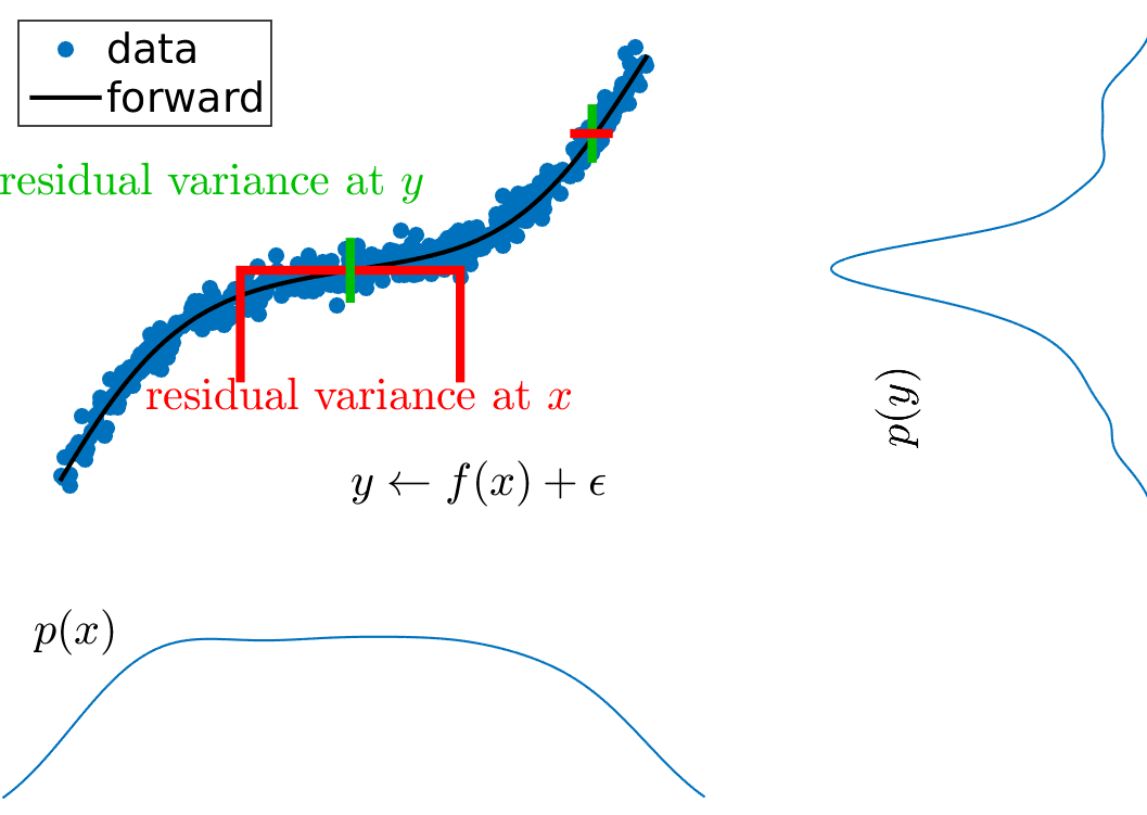
Figure 1: Cause-effect relations can be identified in a deterministic case by looking at the correlation of the slope of $f$ with the density of the cause, $p(x)$. The rationale is that the cause is generated independently from the mechanism mapping it to the effect. Therefore, the shape (slope) of the function should be more uncorrelated with the density of the cause than the other way around. Otherwise, the inverse $f^{-1}$ seems better fitted to the effect density $p(y)$. The density asymmetry is one of the footprints one can use to infer cause-effect relations. When noise is present (blue dots), ANM can be applied here: two models are developed (one that tries to explain $x$ from $y$, and vice versa) and then one looks which one yields residuals more uncorrelated with the potential cause. In this example of $x$ causes $y$, one can see that the residual variance of $x$ depends of $y$ (red bars) while the residual variance at $y$ (green bars) is roughly constant for all $x$, which suggests that is a more plausible model.

II-B Non-deterministic setting

The vast majority of real (and thus more interesting) problems are not deterministic, the function $f$ relating the two variables is not bijective, and $f$ is inaccessible so one cannot compute its derivatives, and from there a criterion of independence between the densities of the cause and the mechanism. An alternative is to rely on the assumption made in Additive Noise Models (ANM) for causal inference [31].

Given two random variables $x$ and $y$ with causal relation $x\to y$, under some conditions, one can demonstrate (cf. e.g. Theorem 4.5 about the identifiability of ANMs in [6]) that there exists an additive noise model

$$y=f(x)+n_{f},$$

in the correct causal direction, but there exists no additive noise model

$$x=g(y)+n_{g}$$

in the anticausal direction. The above mentioned Theorem can be derived through the particular assumptions and it states that generically, a distribution does not admit an ANM in both directions at the same time.

This observation allowed Hoyer et al. [31] to design an algorithm to distinguish cause from effect in pairs of variables from empirical data. Essentially, the methodology performs nonlinear regression from $x\to y$ (and vice versa, $y\to x$) and assesses the independence of the forward, $r_{f}=y-f(x)$, and backward residuals, $r_{b}=x-g(y)$, with the input variables (drivers) $y$ and $x$, respectively. The more independent residuals tell us the right direction of causation.

Relevant assumptions are done in this approach. First, we assume that the considered problem is described accurately looking at the pairs (representational property). Another important assumption is the causal sufficiency, which states that there is no hidden common cause in the considered variables that is causing any of the latter, and thus acts as a confounder. Third, the causal Markov assumption hold, which allows us to treat the causal graph as a probabilistic one. In addition, there are two extra conditions on the regression functions: (i) $f,g$ are either linear and noise is non-Gaussian, or (ii) $f,g$ are nonlinear and output’s densities are positive and smooth [27, 6].

In order to define a practical criterion, two ingredients are needed only: a regression method to learn functions $f$ and $g$, and a powerful dependence estimate to assess the independence of the residuals. Therefore, the framework needs two fundamental blocks: 1) a nonlinear regression model, and 2) a dependence measure. We typically rely on Gaussian Processes [33] and the HSIC [34], respectively. In what follows, we briefly review the theory under these two kernel methods [40]. Then we define the causality criterion.

II-B1 Gaussian Processes (GPs)

Standard regression approximates observations (often referred to as outputs) as the sum of some unknown latent function $f({\mathbf{x}})$ of the input data plus constant power (homoscedastic) Gaussian noise of variance $\lambda^{2}$. Note that in our case, both inputs and outputs are unidimensional, $x,y\in\mathbb{R}$. Therefore, given $n$ input-output data pairs, the dataset is denoted as ${\mathcal{D}}=\{({\mathbf{x}}_{i},{\mathbf{y}}_{i})\}_{i=1}^{n}$, and the model approximation is

$$y_{i}=f({\mathbf{x}}_{i})+\varepsilon_{i},~{}~{}~{}\varepsilon_{i}\sim\mathcal{N}(0,\lambda^{2}).$$ (1)

Instead of proposing a parametric form for $f({\mathbf{x}})$ and learning its parameters in order to fit observed data well, GP regression proceeds in a Bayesian, non-parametric way. A zero mean GP prior is placed on the latent function $f({\mathbf{x}})$ and a Gaussian prior is used for each latent noise term $\varepsilon_{i}$, $f({\mathbf{x}})\;\sim\;\mathcal{GP}(0,k_{\boldsymbol{\mathbf{\theta}}}({\mathbf{x}},{\mathbf{x}}^{\prime}))$, where $k_{\boldsymbol{\mathbf{\theta}}}({\mathbf{x}},{\mathbf{x}}^{\prime})$ is a covariance function parametrized by ${\boldsymbol{\mathbf{\theta}}}$ and $\sigma^{2}$ is a hyperparameter that specifies the noise power. Essentially, a GP is a stochastic process whose marginals are distributed as a multivariate Gaussian. In particular, given the priors $\mathcal{GP}$, samples drawn from $f({\mathbf{x}})$ at the set of locations $\{{\mathbf{x}}_{i}\}_{i=1}^{n}$ follow a joint multivariate Gaussian with zero mean and covariance matrix ${\boldsymbol{\mathbf{K_{\boldsymbol{\mathbf{ff}}}}}}$ with $[{\boldsymbol{\mathbf{K_{\boldsymbol{\mathbf{ff}}}}}}]_{ij}=k_{\boldsymbol{\mathbf{\theta}}}({\mathbf{x}}_{i},{\mathbf{x}}_{j})$.

If we consider a test location ${\mathbf{x}}_{*}$ with corresponding output $y_{*}$, priors $\mathcal{GP}$ induce a prior distribution between the observations ${\bf y}=[y_{1},\ldots,y_{n}]^{\top}$ and $y_{*}$. Now it is possible to analytically compute the posterior distribution over the unknown output $y_{*}$ given the test input ${\mathbf{x}}_{*}$ and the available training set ${\cal D}$,

$$p(y_{*}|{\mathbf{x}}_{*},{\cal D})=\mathcal{N}(y_{*}|\mu_{\text{GP}*},\sigma_{\text{GP}*}^{2}),$$ (2)

which is a Gaussian with the following mean and variance:

$$\mu_{\text{GP}*} ={\boldsymbol{\mathbf{k}}}_{{\boldsymbol{\mathbf{f}}}*}^{\top}({\boldsymbol{\mathbf{K}}}_{{\boldsymbol{\mathbf{ff}}}}+\lambda^{2}{\boldsymbol{\mathbf{I}}}_{n})^{-1}{\boldsymbol{\mathbf{y}}}$$ (3)

$$\sigma_{\text{GP}*}^{2} =\lambda^{2}+k_{**}-{\boldsymbol{\mathbf{k}}}_{{\boldsymbol{\mathbf{f}}}*}^{\top}({\boldsymbol{\mathbf{K}}}_{{\boldsymbol{\mathbf{ff}}}}+\lambda^{2}{\boldsymbol{\mathbf{I}}}_{n})^{-1}{\boldsymbol{\mathbf{k}}}_{{\boldsymbol{\mathbf{f}}}*},$$ (4)

where ${\boldsymbol{\mathbf{k}}}_{{\boldsymbol{\mathbf{f}}}*}=[k({\mathbf{x}}_{*},{\mathbf{x}}_{1}),\ldots,k({\mathbf{x}}_{*},{\mathbf{x}}_{n})]^{\top}\in\mathbb{R}^{n}$ contains the kernel similarities of the test point ${\mathbf{x}}_{*}$ to all training points in ${\cal D}$, ${\boldsymbol{\mathbf{K}}}_{{\boldsymbol{\mathbf{ff}}}}$ is a $n\times n$ kernel (covariance) matrix whose entries contain the similarities between all training points, $\lambda^{2}$ is a hyperparameter accounting for the variance of the noise, $k_{**}=k({\mathbf{x}}_{*},{\mathbf{x}}_{*})$ is a scalar with the self-similarity of ${\mathbf{x}}_{*}$, and ${\boldsymbol{\mathbf{I}}}_{n}$ is the identity matrix of size $n$. Note that both the predictive mean and the variance can be computed in closed-form, and that the predictive variance $\sigma_{\text{GP}*}^{2}$ does not depend on the outputs/target variable.

II-B2 Kernel Dependence Estimation with HSIC

Let us consider two spaces ${\mathcal{X}},{\mathcal{Y}}\subseteq\mathbb{R}$, on which we jointly sample observation pairs $({\mathbf{x}},{\mathbf{y}})$ from distribution $p({\mathbf{x}},{\mathbf{y}})$. The covariance matrix ${\mathcal{C}}_{{\mathbf{x}}{\mathbf{y}}}$ encodes first order dependencies between the random variables. A statistic that efficiently summarizes the content of this matrix is its Hilbert-Schmidt norm. This quantity is zero if and only if there exists no second order dependence between ${\mathbf{x}}$ and ${\mathbf{y}}$.

The nonlinear extension of the notion of covariance was proposed in [34] to cope with higher-order relations between the data. The use of its linear formulation has some limitations and cannot discover more complex relations, for this purposed the use of nonlinear kernel functions allows to capture higher-order effects. Let us define a (possibly non-linear) mapping $\boldsymbol{\phi}$: ${\mathcal{X}}\to{\mathcal{F}}$ such that the inner product between features is given by a positive definite (p.d.) kernel function $K_{x}({\mathbf{x}},{\mathbf{x}}^{\prime})=\langle\boldsymbol{\phi}({\mathbf{x}}),\boldsymbol{\phi}({\mathbf{x}}^{\prime})\rangle$. The feature space ${\mathcal{F}}$ has the structure of a reproducing kernel Hilbert space (RKHS). Let us now denote another feature map $\boldsymbol{\psi}$: ${\mathcal{Y}}\to{\mathcal{G}}$ with associated p.d. kernel function $K_{y}({\mathbf{y}},{\mathbf{y}}^{\prime})=\langle\boldsymbol{\psi}({\mathbf{y}}),\boldsymbol{\psi}({\mathbf{y}}^{\prime})\rangle$. Then, the cross-covariance operator between these feature maps is a linear operator ${\mathcal{C}}_{{\mathbf{x}}{\mathbf{y}}}:{\mathcal{G}}\to{\mathcal{F}}$ such that ${\mathcal{C}}_{{\mathbf{x}}{\mathbf{y}}}={\mathbb{E}}_{{\mathbf{x}}{\mathbf{y}}}[(\boldsymbol{\phi}({\mathbf{x}})-\boldsymbol{\mu}_{x})\otimes(\boldsymbol{\psi}({\mathbf{y}})-\boldsymbol{\mu}_{y})],$ where $\otimes$ is the tensor product, $\boldsymbol{\mu}_{x}={\mathbb{E}}_{{\mathbf{x}}}[\boldsymbol{\phi}({\mathbf{x}})]$, and $\boldsymbol{\mu}_{y}={\mathbb{E}}_{{\mathbf{y}}}[\boldsymbol{\psi}({\mathbf{y}})]$. See more details in [41, 42]. The squared norm of the cross-covariance operator, $\|{\mathcal{C}}_{{\mathbf{x}}{\mathbf{y}}}\|^{2}_{\text{HS}}$, is called the Hilbert-Schmidt Independence Criterion (HSIC) and can be expressed in terms of kernels [34]. Given the set ${\mathcal{D}}$ with $n$ scalar pairs drawn from the joint $p({\mathbf{x}},{\mathbf{y}})$ an empirical estimator of HSIC is [43]:

$$\text{HSIC}=\dfrac{1}{n^{2}}\text{Tr}({\bf H}{\bf K}_{x}{\bf H}~{}{\bf K}_{y}),$$ (5)

where $\text{Tr}(\cdot)$ is the trace operation (the sum of the diagonal entries), ${\bf K}_{x}$, ${\bf K}_{y}$ are the kernel matrices for the input random variables ${\mathbf{x}}$ and ${\mathbf{y}}$, respectively, and ${\bf H}={\bf I}-\frac{1}{n}\mathbbm{1}\mathbbm{1}^{\top}$ centers the data in the feature spaces ${\mathcal{F}}$ and ${\mathcal{G}}$, respectively. It is important to note that HSIC$=0$ occurs if and only if ${\mathbf{x}}$ and ${\mathbf{y}}$ are independent, the proof of this theoretical result is provided on [43].

II-B3 Causal criterion

We build on the ANM approach revised in Section II-B and originally presented in [31] to discover causal association between variables $x$ and $y$. The method provided good results in a set of experiments. A thorough comparison to other methods and in many real and synthetic datasets was conducted in [27]. In general, the best performing criterion to detect the causal direction was simply defined as the difference in test statistic between both forward and backward models:

$$\widehat{C}:=\text{HSIC}(x,r_{f})-\text{HSIC}(y,r_{b})$$ (6)

where $r_{f}=y-f(x)$ and $r_{b}=x-g(y)$ are the residuals yielded by the forward (backward) models $f$ and $g$, respectively. See Section II-B. Intuitively, we compare which method yields more independent residuals (lower HSIC value) as an indicator of model plausibility. The sign of the criterion $\hat{C}$ tells the causal direction: more negative values indicate that the forward model is more plausible and thus one decides that $x$ causes $y$. While other criteria could be adopted, we take this one as the baseline method because of its state-of-the-art performance [27].

II-C An illustrative example

The intuition behind the approach is that statistically significant residuals in one direction indicates the true data-generating mechanism (see Sections §I and §II-A). See an illustrative example in Fig. 2. The problem contains values of altitude and averaged temperature of $n=349$ weather stations in Germany, and the data was provided by the Deutscher Wetterdienst (DWD). The problem reduces to identify the common sense direction of ‘altitude causes temperature’ from the data. Cities are obviously in the troposphere, so under the inversion layer. Nevertheless, a potential confounder is the latitude, since in Germany most of the mountains are in the south, which leads to positive correlations between altitude and temperature. Nevertheless, the direct causal relation between altitude and temperature dominates over the confounder. Following Hoyer’s approach, two GPs were fitted to the forward and backward directions, and we measured the independence of the obtained residuals with both the standard correlation coefficient $\rho$ and the HSIC. Lower independence values are obtained in the forward (causal) direction.

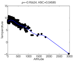
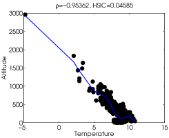
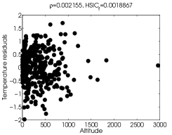
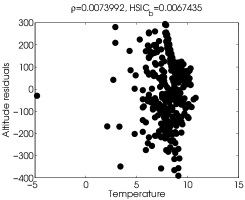
Figure 2: Example of the method in [31] in the altitude causes temperature problem. The fitted functions (top row) are used to approximate $f$ and $g$ models. From here, the particular distribution of the obtained residuals versus the potential cause (bottom) establish the direction of causation as that showing more independent residuals from the driver. We give the correlation coefficient and the HSIC values between the residuals and the potential cause under examination for both the forward and backward models, i.e. between residuals $r_{f}=y-\hat{y}$ and $x$, and between residuals $r_{b}=x-\hat{x}$ and $y$. In this work we focus on HSIC to capture the nonlinear dependence.

III Causal Inference with Sensitivity Maps

HSIC has been used in combination with ANM for causal inference before [44], see Eq. (6). Since the most sensitive points typically dominate the HSIC measure of dependence, we here propose a criterion for causal discrimination in terms of the derivative of the HSIC with respect both the drivers and the residuals in ANM schemes. In the following, we review the main ingredients of the proposed criterion: we give the formulation of the HSIC sensitivity maps, the proposed causality criterion, and study their empirical and theoretical properties.

III-A Sensitivity analysis and maps

A general definition of the sensitivity map (SM) in the context of kernel methods was originally introduced in [45]. Let us define HSIC as a function $h:\mathcal{X}\times\mathcal{Y}\to\mathbb{R}$. The sensitivity map is the expected value of the squared derivative of the function (or the log of the function) with respect the arguments $\mathbbm{z}=(x,y)$. Formally, let us define the sensitivity as

$$s=\int_{\mathcal{Z}}\bigg{(}\dfrac{\partial h(\mathbbm{z})}{\partial z}\bigg{)}^{2}p(\mathbbm{z})\text{d}\mathbbm{z},$$ (7)

where $p(\mathbbm{z})$ is the probability density function over the inputs $\mathbbm{z}\in{\mathcal{Z}}$. Intuitively, the objective of the sensitivity map is to measure the changes of the function $h(\mathbbm{z})$ along the inputs $\mathbbm{z}$. In order to avoid the possibility of cancellation of the terms due to its signs, the derivatives are typically squared, even though other unambiguous transformations like the absolute value could be equally applied. Integration gives an overall measure of sensitivity over the observation space ${\mathcal{Z}}$. The empirical sensitivity map approximation to Eq. (7) is obtained by replacing the integral with a summation over the available $n$ samples

$$s\approx\dfrac{1}{n}\sum_{i=1}^{n}\dfrac{\partial h(\mathbbm{z})}{\partial z}\bigg{|}_{\mathbbm{z}_{i}}^{~{}2}.$$ (8)

Since the HSIC function $h$ works on $(x,y)$, we have to apply this expression twice, which returns the sensitivity vector ${{\boldsymbol{\mathbf{s}}}}=[s^{x},s^{y}]$. This gives the relevance of variables $x$ and $y$ in the function $h$. Alternatively, one can summarize the maps variable-wise to obtain a point-wise relevance:

$$p_{i}=\sqrt{\bigg{(}\dfrac{\partial h(\mathbbm{z})}{\partial x}\bigg{)}^{2}+\bigg{(}\dfrac{\partial h(\mathbbm{z})}{\partial y}\bigg{)}^{2}},$$ (9)

which will be used in this paper to evaluate the relevance of points in the dependence measure. Actually, this way of summarizing the information conveyed by the sensitivity map is somewhat related to the concepts of leveraging and influential points in statistics [46].

III-B Sensitivity maps for the HSIC

In order to derive the sensitivity maps for HSIC which were originally presented in [47], we need to compute its partial derivatives w.r.t. points in variables $x$ and $y$, i.e. $x_{i}$ and $y_{i}$. By applying the chain rule, and first-order derivatives of matrices, we obtain:

$$s_{i}^{x}:=\dfrac{\partial\text{HSIC}}{\partial x_{i}}=-\frac{2}{\sigma^{2}n^{2}}\text{Tr}\left({\bf H}{\bf K}_{y}{\bf H}({\bf K}_{x}\circ{\bf M}_{i}\right)),$$ (10)

where matrix ${\bf M}_{i}$ depends on the $i$-th point sample and it is formed by zeroes except in the $i$-th column which corresponds to $\text{vec}(x_{i})-{\mathbf{x}}$ ($i$-th element minus vector ${\mathbf{x}}$).

$$s_{i}^{y}:=\dfrac{\partial\text{HSIC}}{\partial y_{i}}=-\frac{2}{\sigma^{2}n^{2}}\text{Tr}\left({\bf H}{\bf K}_{x}{\bf H}({\bf K}_{y}\circ{\bf N}_{i})\right),$$ (11)

where matrix ${\bf N}_{i}$ depends on the $i$-th point sample and it is formed by zeroes except in the $i$-th column which corresponds to $\text{vec}(y_{i})-{\mathbf{y}}$ ($i$-th element minus vector ${\mathbf{y}}$). The joint sensitivity map is defined as the concatenation of individual sensitivities, ${{\boldsymbol{\mathbf{s}}}}=[s^{x},s^{y}]$, where $s^{x}=\frac{1}{n}\sum_{i=1}^{n}(s_{i}^{x})^{2}$ and $s^{y}=\frac{1}{n}\sum_{i=1}^{n}(s_{i}^{y})^{2}$; and the point-wise sensitivity as $p_{i}=\sqrt{(s_{i}^{x})^{2}+(s_{i}^{y})^{2}}$.

III-C Proposed causal criterion with sensitivity maps

We here propose an alternative criterion for bivariate causality based on the sensitivity maps of HSIC in both directions:

$$\widehat{C}_{s}:=(s_{b}^{y}+s_{b}^{r})-(s_{f}^{x}+s_{f}^{r}),$$ (12)

where subscripts $f$ and $b$ stand for the forward and backward directions respectively, and the superscripts refer to the sensitivities of either the observations $x$ and $y$, or the corresponding residuals, $r_{f}$ and $r_{b}$. The criterion now accounts for the relative relevance of points and residuals in the dependence estimate according to the sensitivity measure. Besides, note the intuitive connection to the deterministic case in section II-A. Here we do not focus on the derivative of the underlying function, but the derivative of the dependence estimate itself [39]. Following the same “altitude causes temperature” example, we show in Fig. 3 the point sensitivities in the distributions. It becomes clearer the structured (more dependent) distribution in the backward direction (Fig. 3[right]), which suggests that the forward direction is the causal one.

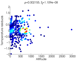
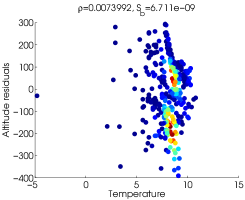
Figure 3: Sensitivity maps of the points most affecting the independence measure (follow-up from example in section II-C). Colors reflect the importance of the particular example in the dependence measure (HSIC), as computed with the sensitivity map.

(a)	(b)	(c)

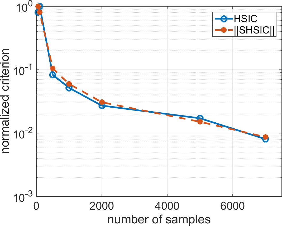
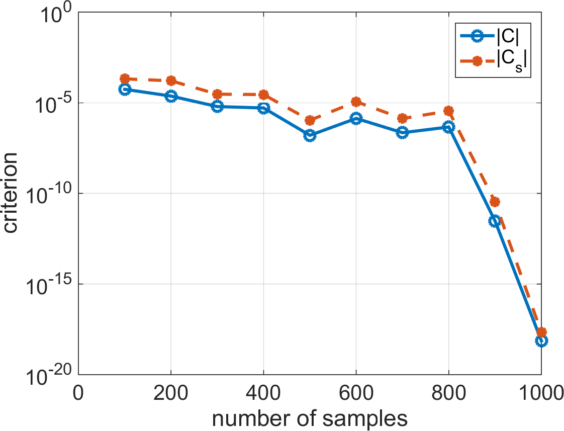
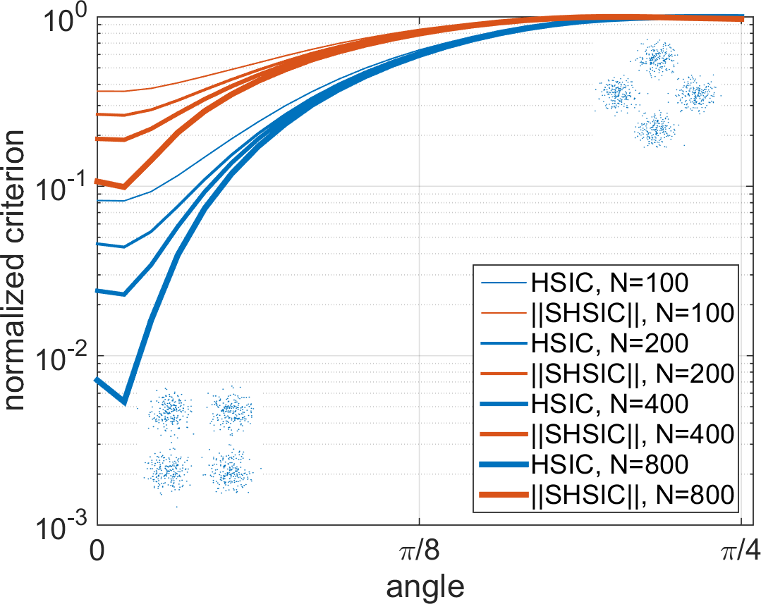
Figure 4: Convergence of (a) the HSIC and the norm of its sensitivity map; (b) the criteria for causal detection, both under the independence hypothesis. Data are drawn from uniform distributions independently, $x,y\sim{\mathcal{U}}(0,1)$ with different number of samples. Both estimators converge to zero with the number of samples at similar rates. (c) Convergence of the criteria under the hypothesis of varying dependence. We generate different problems from independence (left) to dependence (right) by rotating the X-OR gate for different angles, $\theta\in$[$0,\pi/4$]. We show the HSIC and the norm of the HSIC sensitivity maps when varying the $\theta$ angle.

III-D Consistency Properties

Let us now study the consistency properties of proposed criterion. Following [44], a plausible criterion of causality for ANMs has to rely on a consistent dependence criterion, and the combination of the ANM and the dependence estimator should be consistent too.
Let us show first that the norm of the sensitivity map acts as a consistent dependence measure. Note that in [31] originally proposed to use the $p$-value of HSIC to define the causality criterion which leads to a consistent procedure, and in [44] it is shown that the same happens for the HSIC itself. Therefore, we have to ensure here that the norm of the sensitivity maps acts as a consistent dependence measure. It is customary to consider that if an estimator $\rho(X,Y)$ fulfills that “$\rho^{\ast}$(X,Y)$=0$ iff $X$ and $Y$ are statistically independent”, then it is considered a dependence measure. Let us first give an empirical demonstration that the norm of the sensitivity maps of HSIC is a consistent estimator: under the hypothesis of independence (Fig. 4[a-b]) both HSIC and $\|$SHSIC$\|$ converge to zero with $N$; while in an example of increasing dependence (Fig. 4[c]) convergence is ensured too.
In theoretical terms, to ensure consistency of the proposed criterion, we must demonstrate that for each of the four terms in

$$\widehat{C}_{s}:=C_{b}-C_{f}=(s_{b}^{y}+s_{b}^{r})-(s_{f}^{x}+s_{f}^{r}).$$

We will show it for the forward term $C_{f}$, the same arguments apply for $C_{b}$:

$$C_{f}(x,r):=s_{f}^{x}+s_{f}^{r}=\|\partial_{x}\text{HSIC}\|^{2}+\|\partial_{r}\text{HSIC}\|^{2}.$$

Note that for real numbers, the norm of the sensitivity maps of HSIC should be Lipschitz continuous to ensure convergence, that is, we need to demonstrate $|C_{f}(x,r)-C_{f}(x,r^{\prime})|\leq L\|r-r^{\prime}\|$. For that, we can show that a multivariate function $f:\mathbb{R}^{D}\to\mathbb{R}$ with bounded partial derivatives, which is our case, is Lipschitz, and that the bound is exactly $L=\sqrt{2}\max_{i}(\sup|\partial_{r_{i}}\text{HSIC}|)$, $i=1,\ldots,N$. This is an equivalent result to Lemma 16 in [44] for the HSIC sensitivity map.
The second condition to fulfill is that the norm of the sensitivity map in ANMs should be consistent. This can be demonstrated following the same procedure that the one in Theorem 20 (Appendix A.3) in [44] for HSIC, and using the previous consistency lemma for the proposed estimator here.

III-E Computational cost and efficient criterion

Note that both HSIC and its sensitivity map give raise to closed-form solutions, just involving simple matrix multiplication and a trace operation. Both HSIC and its sensitivity scale quadratically with the number of examples $N$ since the involved kernel matrices and the centering matrix are $N\times N$. This makes both HSIC and its sensitivity map unfeasible with moderate to large datasets. In [47] we provided with fast versions of both HSIC and its sensitivity map through the use of random Fourier features. The cost of a naive implementation of HSIC is ${\mathcal{O}}(N^{3})$, and its randomized version is ${\mathcal{O}}(D^{3})$, where $D$ is the number of Fourier features chosen to approximate the kernel matrices, which is typically smaller than the number of points, i.e. $D\ll N$. Respectively, the naive implementation of the sensitivity of HSIC is ${\mathcal{O}}(N^{3}+N^{2})\approx{\mathcal{O}}(N^{3})$ and its randomized version scales as ${\mathcal{O}}(D^{3}+D^{2}N)$ so in the cases of $N\gg D$ the cost reduces to ${\mathcal{O}}(D^{2}N)$. The cost of the causal criteria is thus defined by these operations. In addition, we demonstrated the convergence of both the randomized HSIC to HSIC, and their corresponding sensitivity maps, which allows a practical use of the method.

IV Results

In this section we show the performance of the proposed methodology in three experimental settings: (1) in a collection of 28 geoscience causal inference problems, (2) in a database of radiative transfer models simulations and machine learning emulators in Sentinel-2 vegetation parameter modeling conforming a set of 182 causal problems with groundtruth, and (3) in assessing the impact of different regression models based on GPs in discovering causality in Net Ecosystem Production variables. All problems are bivariate and a annotated ground truth is available based on expert knowledge or common sense, which allows us to assess performance quantitatively.

We quantify the accuracy in detecting the direction of causation using standard scores like the receiver operating curves (ROC), precision-recall curves (PRC) curves, and the areas under these curves. We compare in all cases the state-of-the-art criterion in (6) with our criterion in (12). Methods performance are also studied under different situations of number of available points, presence of different noise sources and distortions, and impact of different GP regression models on the detection accuracy.

ıin 1,2,3,4,20,21,42,43,44,45,46,49,50,51,72,73,78,79,80,81,82,83,87,89,90,91,92,93

Figure 5: Scatter plots in the CEP benchmark dataset. See a brief description of all individual problems in Table I and more details in [27].

IV-A Experiment 1: Geoscience Cause Effect Pairs

TABLE I: Problems and causal direction for the geoscience problems in the CEP database.

id	$x$	$y$	Cause
01	Altitude	Temperature	$\rightarrow$
02	Altitude	Precipitation	$\rightarrow$
03	Longitude	Temperature	$\rightarrow$
04	Altitude	Sunshine hours	$\rightarrow$
20	Latitude	Temperature	$\rightarrow$
21	Longitude	Precipitation	$\rightarrow$
42	Day of the year	Temperature	$\rightarrow$
43	Temperature at $t$	Temperature at $t+1$	$\rightarrow$
44	Pressure at $t$	Pressure at $t+1$	$\rightarrow$
45	Sea level pressure at $t$	Sea level pressure at $t+1$	$\rightarrow$
46	Relative humidity at $t$	Relative humidity at $t+1$	$\rightarrow$
49	Ozone concentration	Temperature	$\leftarrow$
50	Ozone concentration	Temperature	$\leftarrow$
51	Ozone concentration	Temperature	$\leftarrow$
72	Sunspots	Global mean temperature	$\rightarrow$
73	CO2 emissions	Energy use	$\leftarrow$
77	Temperature	Solar radiation	$\leftarrow$
78	PPFD	Net Ecosystem Productivity	$\rightarrow$
79	NEP	Diffuse PPFDdif	$\leftarrow$
80	NEP	Diffuse PPFDdif	$\leftarrow$
81	Temperature	Local CO2 flux, BE-Bra	$\rightarrow$
82	Temperature	Local CO2 flux, DE-Har	$\rightarrow$
83	Temperature	Local CO2 flux, US-PFa	$\rightarrow$
87	Temperature	Total snow	$\rightarrow$
89	root decomposition	root decomposition (grassland)	$\leftarrow$
90	root decomposition	root decomposition (forest)	$\leftarrow$
91	clay content in soil	soil moisture	$\rightarrow$
92	organic carbon in soil	clay cont. in soil (forest)	$\leftarrow$
93	precipitation	runoff	$\rightarrow$
94	hour of day	temperature	$\rightarrow$

We used Version 1.0 of the CauseEffectPairs (CEP) collection freely. The database contains 100 pairs of random variables along with the right direction of causation (ground truth). Data has been collected from various domains of application, such as biology, climate science, health sciences and economics, just to name a few. More information about the dataset and an excellent up-to-date review of observational causal inference methods is available in [27]. We conducted experiments in 28 out of the 100 pairs that contain one-dimensional variables and that are related to geosciences and remote sensing: problems involving carbon and energy fluxes, ecological indicators, vegetation indices, temperature, moisture, heat, etc. We summarize the involved variables in Table I, and show the scatter plots of the selected pairs $(x,y)$ in Fig. 5.

IV-A1 Experimental Setup

The experimental setting is as follows. Once the two predictive models $f$ and $g$ were developed, we computed the two HSIC terms, as well as their sensitivity maps between the $x$ (or $y$) and the residuals $r_{f}$ (or $r_{b}$). The final causal direction score was simply defined as the difference in test statistic between both models, either using $\hat{C}$ or the proposed $\hat{C}_{s}$. Note that this is a particular form of ‘ranked-decision’ setting that needs to account for the bias introduced by pairs coming from the same problem, i.e. it is customary to down-weight the precision for every decision threshold in the curves (e.g. four related problems receive 0.25 weights in the decision). This is the case, for example of problems 81, 82, 83 and 87 that receive 0.25 weights.

IV-A2 Accuracy and robustness of the detection

We run the experiments with different numbers of (randomly selected) points $n$ from both variables. This situation impacts regression models performance, both in terms of the regression accuracy and the dependence estimation. We evaluate $\hat{C}$ and $\hat{C}_{s}$ criteria by limiting the maximum number of training samples in each problem, $n_{max}=\{50,100,200,500,2000\}$. Results were averaged over $10$ realizations. Figure 6 shows the AUC under the curve as a function of $n_{max}$. The proposed sensitivity-based criterion consistently performed better than the standard approach using HSIC alone. Lower values of AUC are obtained by our proposal only when the number of samples is relatively low (50 and 100). This particular behavior is plausible because our criterion is defined through an empirical estimator (the sensitivity) and when the number of samples is moderately low it can give rise to underestimated values. Looking more in detail at the ROC in Fig. 7, we note that the proposed $\hat{C}_{s}$ yields the best recognition curves, both ROC and the PRC. Note that this happens for all decision rates, especially in low false positive rates regimes, and for all number of training points.

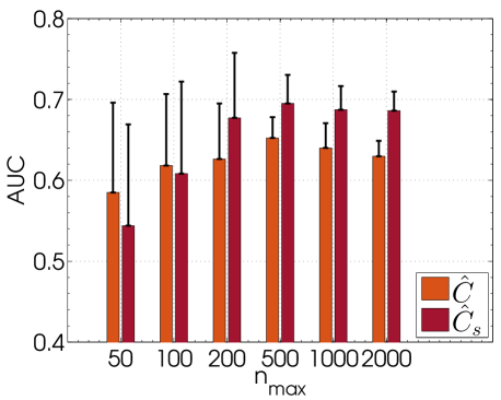
Figure 6: AUCs in the CEP causality problems dataset for different amounts of training data per problem.

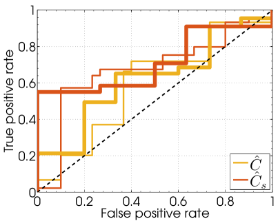
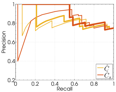
Figure 7: Receiver operating curve (ROC) (top) and Precision-Recall (PR) (bottom) curves for the causality problems in the Geoscience Cause Effect Pairs (experiment section 1) using $n=200$ (thin lines) and $n=2000$ (thick lines). Higher area under the curves are obtained with the proposed criterion $C_{s}$ and for both situations.

IV-B Experiment 2: Causation in RTM assessment

Using input-output data pairs generated by radiative transfer models (RTMs) allow us to assess performance of observational causality algorithms: it is obvious that the forward RTM simulation gives the right direction of causation: state vectors (parameters) cause radiances and not the other way around. The strength of the causation is not considered here. In this second experiment, we deal with data generated by the standard PROSAIL RTM. PROSAIL is the combination of the PROSPECT leaf optical properties model and the SAIL canopy bidirectional reflectance model. PROSAIL has been used to develop new methods for retrieval of vegetation biophysical properties. Essentially, PROSAIL links the spectral variation of canopy reflectance, which is mainly related to leaf biochemical contents, with its directional variation, which is primarily related to canopy architecture and soil/vegetation contrast. This link is key to simultaneous estimation of canopy biophysical/structural variables for applications in agriculture, plant physiology, and ecology at different scales. PROSAIL has become one of the most popular radiative transfer tool due to its ease of use, robustness, and consistent validation by lab/field/space experiments over the years.

TABLE II: Configuration parameters of the simulated data.

Parameter	Sampling	Min	Max
RTM model: Prospect 4
Leaf Structural Parameter	Fixed	1.50	1.50
Cab, chlorophyll a+b [$\mu$g/cm2]	${\mathcal{U}}(14,49)$	0.067	79.97
Cw, equivalent water thickness [mg/cm2]	${\mathcal{U}}(10,31)$	2	50
Cm, dry matter [mg/cm2]	${\mathcal{U}}(5.9,19)$	1.0	3.0
RTM model: 4SAIL
Diffuse/direct light	Fixed	10	10
Soil Coefficient	Fixed	0	0
Hot spot	Fixed	0.01	0.01
Observer zenit angle	Fixed	0	0
LAI, Leaf Area Index	${\mathcal{U}}(1.2,4.3)$	0.01	6.99
LAD, Leaf Angle Distribution	${\mathcal{U}}(28,51)$	20.04	69.93
SZA, Solar Zenit Angle	${\mathcal{U}}(8.5,31)$	0.082	49.96
PSI, Azimut Angle	${\mathcal{U}}(30,100)$	0.099	179.83

IV-B1 Experimental Setup

We used PROSAIL to generate $n=1000$ pairs of Sentinel-2 spectral (13 spectral channels) by varying 7 parameters in reasonable ranges: Total Leaf Area Index (LAI), Leaf angle distribution (LAD), Solar Zenit Angle (SZA), Azimut Angle (PSI), chlorophyll a+b content $C_{ab}$ [$\mu$g/cm²], equivalent water thickness $C_{w}$ [g/cm²] and dry matter content, $C_{m}$ [g/cm²]. Several parameters were kept fixed in the simulations. See Table II for the configuration details used in our PROSAIL simulations. Building the database assumes that every individual parameter impacts (causes) a particular spectral channel, and that spectral channels cannot cause the parameters. This returns a simulated dataset with $2\times 13\times 7=182$ causal problems with ground truth.

IV-B2 Accuracy and robustness of the detection

We run the different criteria and obtained the corresponding ROCs and AUCs. We did observe very high accuracy levels for all criteria. We then assessed robustness of the methods to different additive white Gaussian noise levels, varying the SNR in the range [0,40] dB. Figure 8 shows the obtained results for all causal criteria and accuracy measures as a function of SNR. Our proposed criterion $\widehat{C}_{s}$ shows better performance than $\widehat{C}$ for all SNR levels, with an average improvement of +5% in AUC. Both criteria degrade in scenarios dominated by noise (SNR$<$10dB), where neither the functions nor independence can be estimated correctly.

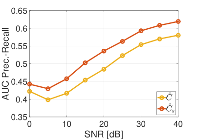
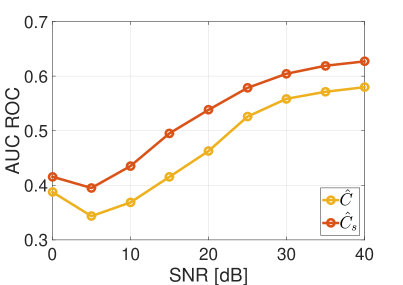
Figure 8: Area under the curve (AUC) of Precision-Recall (top) and AUC of the ROC curves (bottom) both against the amount of noise included in the experiments. Higher detection power is obtained with the proposed $C_{s}$ for all noise levels and measures.

IV-C Experiment 3: Causation in RTM Emulation

As observed before, noise plays a fundamental role in causal discovery. In this experiment we studied the impact of other types of distortions in remote sensing data. In particular, we aim to assess the non-linearities introduced when approximating a physical model via machine learning. This form of surrogate modelling is known in the literature as emulation, and has captured the attention in recent years because it allows to replace RTMs with more efficient statistical algorithms [33, 48]. Emulators, however are just function approximators and the simulated radiances are subject to complicated distortions. We evaluate the identifiability of the causal links in such cases.

Here we trained a neural network using the $n=1000$ points generated by PROSAIL in the previous experiment to build an emulator. Performance showed less than 5% of normalized RMSE in all bands. Once trained, the emulator was run to generate $n=10^{6}$ samples. The same amount of 182 cause-effect bivariate problems as before was generated. We run the different criteria training the regression models with different amounts of data points, $n=\{10000,20000,30000\}$, and the standard AUC and PR criteria are shown in Fig. 9. Results show that (1) all criteria improve performance with an increasing amount of data, and (2) our criterion $\widehat{C}_{s}$ outperforms the state-of-the-art $\widehat{C}$ in all cases (by around +2-4%).

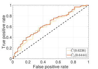
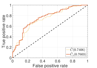
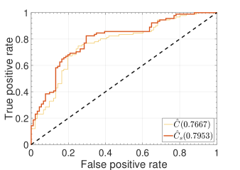
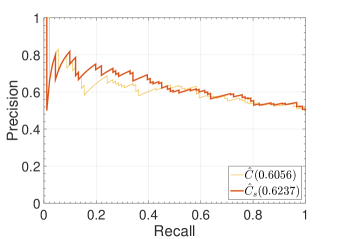
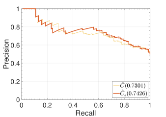
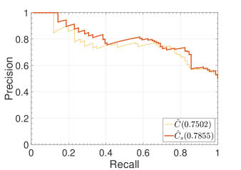
Figure 9: ROC (top row) and Precision-Recall (bottom row) curves for the emulation database of 182 causality problems.

IV-D Experiment 4: Impact of the regression model

In this last experiment, we are concerned about the use of different regression algorithms that better account for noise and non-linearities [33]. In particular, we will compare the use of the standard (homoscedastic) GP regression model (GP) [32] (cf. Section II), with the heteroscedastic GP model (VHGP) introduced in [49, 33] (which accounts for signal-to-noise relations), and a warped GP model (WGP) introduced in [50, 51] (which further transforms model’s output to look more like a Gaussian process).

We exemplify these different approaches in a relevant geoscience problem. Terrestrial ecosystems absorb approximately 120 Gt of carbon annually from the atmosphere, about half is returned as plant respiration and the remaining 60 Gt yr^-1 represent the Net Primary Production (NPP). Out of this, about 50 Gt yr^-1 are returned to the atmosphere as soil/litter respiration or decomposition processes, while about 10 Gt yr^-1 results in the Net Ecosystem Production (NEP). The problem here deals with estimating the causal relation between the photosynthetic photon flux density (PPFD), which is a measure of light intensity, and the NEP, which results from the potential of ecosystems to sequestrate atmospheric carbon. Discovering such relations may be helpful to better understand the carbon fluxes and to establish sinks and sources of carbon. We use here three data sets taken at a flux tower at site DE-Hai involving PPFD(total), PPFD(diffuse), PPFD(direct) drivers and the NEP consequence variable [52].

Results for all three scenarios are shown in Table III. We show the values of HSIC in forward and backward directions, as well as the criteria obtained by all regression models. The heteroscedastic GP accounts for the signal-to-noise relations in a more sensible way, so the dependency estimate becomes slightly more reliable. Nevertheless performance of WGP excels in these particular problems, probably because of the better estimation of conditionals in higher density regions (see Fig. 1 in [53]). Future work will involve testing these models in a wider range of applications.

TABLE III: Results in the ‘PPFD causes NEP’ causal problem.

Method	HSICf	HSICb	$C$	$C_{s}$	Conclusion
GP	6.7525	10.5255	3.7729	-1.9204	PPFD(tot)$\to$ NEP
VHGP	6.8220	11.7661	4.9441	-1.8758	PPFD(tot)$\to$ NEP
WGP	6.8670	12.0412	5.1742	-1.6784	PPFD(tot)$\to$ NEP
GP	8.0982	2.1020	-5.9961	0.8917	NEP $\leftarrow$ PPFD(diff)
VHGP	8.1556	2.1865	-5.9691	0.8674	NEP $\leftarrow$ PPFD(diff)
WGP	8.1707	2.0475	-6.1232	0.7270	NEP $\leftarrow$ PPFD(diff)
GP	11.4727	1.5806	-9.8920	-0.7110	PPFD(dir)$\to$ NEP
VHGP	13.0462	1.6848	-11.3614	-0.6062	PPFD(dir)$\to$ NEP
WGP	13.0061	1.6028	-11.4033	-0.8046	PPFD(dir)$\to$ NEP

V Conclusions

This paper introduced for the first time the issue of observation-based causal inference in bivariate instantaneous problems in remote sensing and geosciences. Approaching this kind of problems requires taking some (strong) assumptions, so results must be taken with extreme caution. Nevertheless, the obtained results confirm that in general causal detection accuracy is well above chance, and opens the field to further experimentation.

To tackle this challenging problem, we used a simple method based on regression and dependence estimation, and proposed a new criterion based on the sensitivity (derivative) of the dependence estimator instead of the dependence itself. This allows us to better capture the asymmetry of the forward and inverse densities with regard to the causal mechanism.

State-of-the-art accuracy was obtained in a wide range of situations with known ground truth. We illustrated performance in a collection of 28 geoscience causal inference problems, in a large database of PROSAIL simulations and emulators in vegetation parameter modeling, and in a carbon cycle problem. We evaluated the impact of using different regression models based on Gaussian Processes; as well as assessed identifiability in the presence of different noise sources and distortions. Models performance was evaluated in global terms by measuring the right direction of causation using standard metrics derived from detection curves.

We would like to finally note that the methodologies proposed here were originally introduced for general-purpose applications. We have nevertheless shown its applicability in remote sensing and geosciences. We relied on a general assumption of structural models in general and ANM in particular. If the assumptions are not fulfilled, the method should not perform well. This may happen in some cases, such as in cases of post-nonlinear effects. Actually, we showed this case experimentally where several regression models were used. The WGP generalizes does not assume an additive noise model in general and results actually confirm that, by replacing the regression model, one can achieve more robust results in cases where assumptions are not met.

The proposed scheme for bivariate causal inference can actually include many independence criteria, such as e.g. differential entropies, empirical Bayes scores or minimum message length scores. We however restricted ourselves to the (standard use of) HSIC, and included a novel causal criterion (the sensitivity map) that can be computed analytically from HSIC. Other more sophisticated criteria could be actually derived from the combination of the sensitivity map and the HSIC values and $p$-values, which will be matter of future research.

Adrián Pérez-Suay obtained his B.Sc. degree in Mathematics (2007), a Master degree in Advanced Computing and Intelligent Systems (2010) and a Ph.D. degree in Computational Mathematics and Computer Science (2015), all from the Universitat de València. He is assistant professor in the Dept. of Mathematics in the Universitat de València. He is currently a Postdoctoral Researcher at the Image and Signal Processing (ISP) working on dependence estimation, kernel methods and causal inference for remote sensing data analysis.

Gustau Camps-Valls (M’04, SM’07, FM’18) received a PhD in Physics in 2002 from the Universitat de València, and he is currently Full professor in Electrical Engineering, and coordinator of the Image and Signal Processing (ISP) group in the same university, http://isp.uv.es. He is interested in the development of machine learning algorithms for geoscience and remote sensing data analysis.

References

- [1] W. G. Cochran and S. P. Chambers, “The planning of observational studies of human populations,” Journal of the Royal Statistical Society. Series A (General), vol. 128, no. 2, pp. 234–266, 1965.
- [2] IPCC, “2014: Climate Change 2014: Synthesis Report. Contribution of Working Groups I, II and III to the Fifth Assessment Report of the Intergovernmental Panel on Climate Change [Core Writing Team, R.K. Pachauri and L.A. Meyer (eds.)]. IPCC,” Switzerland, p. 151, 2014.
- [3] D. Adam, “Climate change in court,” Nature Clim. Change, vol. 1, no. 10, pp. 127–130, 2011.
- [4] J. Pearl, Causality: Models, Reasoning and Inference, 2nd ed. New York, NY, USA: Cambridge University Press, 2009.
- [5] P. Spirtes, C. Glymour, and R. Scheines, Causation, Prediction, and Search, 2nd ed. MIT press, 2000.
- [6] J. Peters, D. Janzing, and B. Schölkopf, Elements of Causal Inference - Foundations and Learning Algorithms, ser. Adaptive Computation and Machine Learning Series. Cambridge, MA, USA: MIT, 2017.
- [7] E. Rastetter, “Validating models of ecosystem response to global change,” Bioscience, vol. 46, no. 3, Mar 1996.
- [8] G. Hegerl and F. Zwiers, “Use of models in detection and attribution of climate change,” Wiley Interdisciplinary Reviews: Climate Change, vol. 2, no. 4, pp. 570–591, 2011.
- [9] U. Triacca, A. Attanasio, and A. Pasini, “Anthropogenic global warming hypothesis: testing its robustness by granger causality analysis,” Environmetrics, vol. 24, no. 4, pp. 260–268, 2013.
- [10] T. Richardson and P. Spirtes, “Ancestral graph markov models,” Ann. Statist., vol. 30, no. 4, pp. 962–1030, 08 2002.
- [11] J. Zhang, “Causal reasoning with ancestral graphs,” Journal of Machine Learning Research, vol. 9, pp. 1437–1474, 2008.
- [12] G.-R. Walther, E. Post, P. Convey, A. Menzel, C. Parmesan, T. J. C. Beebee, J.-M. Fromentin, O. Hoegh-Guldberg, and F. Bairlein, “Ecological responses to recent climate change,” Nature, vol. 416, no. 6879, pp. 389–395, March 2002.
- [13] C. Granger, “Investigating causal relations by econometric models and cross-spectral methods,” Econometrica, vol. 37, no. 3, pp. 424–38, 1969.
- [14] U. Triacca, “Is granger causality analysis appropriate to investigate the relationship between atmospheric concentration of carbon dioxide and global surface air temperature?” Theoretical and Applied Climatology, vol. 81, no. 3, pp. 133–135, 2005.
- [15] D. A. Smirnov and I. I. Mokhov, “From granger causality to long-term causality: Application to climatic data,” Physical Review E, vol. 80, no. 1.
- [16] L. M. W. Leggett and D. A. Ball, “Granger causality from changes in level of atmospheric ; to global surface temperature and the el niño-southern oscillation, and a candidate mechanism in global photosynthesis,” Atmospheric Chemistry and Physics, vol. 15, no. 20, pp. 11 571–11 592.
- [17] G. D. Salvucci, J. A. Saleem, and R. Kaufmann, “Investigating soil moisture feedbacks on precipitation with tests of granger causality,” Advances in water Resources, vol. 25, no. 8, pp. 1305–1312.
- [18] T. J. Mosedale, D. B. Stephenson, M. Collins, and T. C. Mills, “Granger causality of coupled climate processes: Ocean feedback on the north atlantic oscillation,” Journal of climate, vol. 19, no. 7, pp. 1182–1194.
- [19] C. Papagiannopoulou, D. G. Miralles, S. Decubber, M. Demuzere, N. E. C. Verhoest, W. A. Dorigo, and W. Waegeman, “A non-linear Granger-causality framework to investigate climate–vegetation dynamics,” Geoscientific Model Development, vol. 10, no. 5, pp. 1945–1960, 2017.
- [20] P. Spirtes, C. Glymour, and R. Scheines, Causation, prediction, and search. MIT press, 1993.
- [21] I. Ebert-Uphoff and Y. Deng, “Causal discovery for climate research using graphical models,” Journal of Climate, vol. 25, no. 17, pp. 5648–5665.
- [22] J. Runge, V. Petoukhov, J. F. Donges, J. Hlinka, N. Jajcay, M. Vejmelka, D. Hartman, N. Marwan, M. Paluš, and J. Kurths, “Identifying causal gateways and mediators in complex spatio-temporal systems,” Nature Communications, vol. 6, p. 8502, 2015.
- [23] I. Ebert-Uphoff and Y. Deng, “A new type of climate network based on probabilistic graphical models: Results of boreal winter versus summer: climate network based on graphical model,” no. 19.
- [24] C. F. Schleussner, J. Runge, J. Lehmann, and A. Levermann, “The role of the north atlantic overturning and deep ocean for multi-decadal global-mean-temperature variability,” Earth System Dynamics, vol. 5, no. 1, pp. 103–115.
- [25] M. Kretschmer, D. Coumou, J. F. Donges, and J. Runge, “Using causal effect networks to analyze different arctic drivers of midlatitude winter circulation,” Journal of Climate, vol. 29, no. 11, pp. 4069–4081.
- [26] J. Runge, V. Petoukhov, and J. Kurths, “Quantifying the strength and delay of climatic interactions: The ambiguities of cross correlation and a novel measure based on graphical models,” Journal of Climate, vol. 27, no. 2, pp. 720–739.
- [27] J. M. Mooij, J. Peters, D. Janzing, J. Zscheischler, and B. Schölkopf, “Distinguishing cause from effect using observational data: Methods and benchmarks,” Journal of Machine Learning Research, vol. 17, pp. 32:1–32:102, 2016.
- [28] P. Spirtes and K. Zhang, “Causal discovery and inference: concepts and recent methodological advances,” Applied Informatics, vol. 3, no. 1.
- [29] P. Daniusis, D. Janzing, J. Mooij, J. Zscheischler, B. Steudel, K. Zhang, and B. Schölkopf, “Inferring deterministic causal relations,” in UAI, ser. UAI. USA: AUAI Press, 2010, pp. 143–150.
- [30] N. Shajarisales, D. Janzing, B. Schoelkopf, and M. Besserve, “Telling cause from effect in deterministic linear dynamical systems,” in ICML, ser. Proceedings of Machine Learning Research, F. Bach and D. Blei, Eds., vol. 37. Lille, France: PMLR, 07–09 Jul 2015, pp. 285–294.
- [31] P. O. Hoyer, D. Janzing, J. M. Mooij, J. Peters, and B. Schölkopf, “Nonlinear causal discovery with additive noise models,” in NIPS, D. Koller, D. Schuurmans, Y. Bengio, and L. Bottou, Eds., 2008, pp. 689–696.
- [32] C. E. Rasmussen and C. K. I. Williams, Gaussian Processes for Machine Learning. New York: The MIT Press, 2006.
- [33] G. Camps-Valls, J. Verrelst, J. Munoz-Mari, V. Laparra, F. Mateo-Jiménez, and J. Gomez-Dans, “A survey on gaussian processes for earth observation data analysis,” IEEE Geoscience and Remote Sensing Magazine, vol. 4, no. 6, June 2016.
- [34] A. Gretton, R. Herbrich, and A. Hyvärinen, “Kernel methods for measuring independence,” Journal of Machine Learning Research, vol. 6, pp. 2075–2129, 2005.
- [35] G. Camps-Valls, J. Mooij, and B. Scholkopf, “Remote sensing feature selection by kernel dependence measures,” IEEE Geosc. Rem. Sens. Lett., vol. 7, no. 3, pp. 587 –591, Jul 2010.
- [36] G. Camps-Valls, D. Tuia, V. Laparra, and J. Malo, “Estimating biophysical variable dependences with kernels,” in IEEE International Geoscience and Remote Sensing Symposium, 2010, pp. 828–831.
- [37] A. Pérez-Suay and G. Camps-Valls, “Causal inference in geosciences with kernel sensitivity maps,” in IEEE International Geoscience and Remote Sensing Symposium, Fort Worth, Texas, USA, 2017, pp. 763–766.
- [38] D. Janzing, J. Mooij, K. Zhang, J. Lemeire, J. Zscheischler, P. Daniušis, B. Steudel, and B. Schölkopf, “Information-geometric approach to inferring causal directions,” Artif. Intell., vol. 182-183, pp. 1–31, May 2012.
- [39] P. Daniušis, D. Janzing, J. Mooij, J. Zscheischler, B. Steudel, K. Zhang, and B. Schölkopf, “Inferring deterministic causal relations,” in UAI’10.
- [40] G. Camps-Valls and L. Bruzzone, Eds., Kernel methods for Remote Sensing Data Analysis. UK: Wiley & Sons, Dec 2009.
- [41] C. Baker, “Joint measures and cross-covariance operators,” Transactions of the American Mathematical Society, vol. 186, pp. 273–289, 1973.
- [42] K. Fukumizu, F. R. Bach, and M. I. Jordan, “Dimensionality reduction for supervised learning with reproducing kernel Hilbert spaces,” Journal of Machine Learning Research, vol. 5, pp. 73–99, 2004.
- [43] A. Gretton, O. Bousquet, A. Smola, and B. Schölkopf, “Measuring statistical dependence with hilbert-schmidt norms,” in Algorithmic Learning Theory, ser. LNCS, S. Jain, H. Simon, and E. Tomita, Eds. Springer Berlin Heidelberg, 2005, vol. 3734, pp. 63–77.
- [44] J. M. Mooij, J. Peters, D. Janzing, J. Zscheischler, and B. Schölkopf, “Distinguishing cause from effect using observational data: Methods and benchmarks,” J. Mach. Learn. Res., vol. 17, no. 1, pp. 1103–1204, Jan. 2016.
- [45] U. Kjems, L. K. Hansen, J. Anderson, S. Frutiger, S. Muley, J. Sidtis, D. Rottenberg, and S. C. Strother, “The Quantitative Evaluation of Functional Neuroimaging Experiments: Mutual Information Learning Curves,” NeuroImage, vol. 15, no. 4, pp. 772–786, 2002.
- [46] J. Burt, G. Barber, and D. Rigby, Elementary Statistics for Geographers. Guilford Press, 2009.
- [47] A. Pérez-Suay and G. Camps-Valls, “Sensitivity maps of the hilbert–schmidt independence criterion,” Applied Soft Computing, 2017.
- [48] J. P. Rivera, J. Verrelst, J. Gómez-Dans, J. Muñoz-Marí, J. Moreno, and G. Camps-Valls, “An emulator toolbox to approximate radiative transfer models with statistical learning,” Remote Sensing, vol. 7, no. 7, pp. 9347–9370, 2015.
- [49] M. Lázaro-Gredilla and M. K. Titsias, “Variational heteroscedastic gaussian process regression,” in 28th International Conference on Machine Learning, ICML 2011. Bellevue, WA, USA: ACM, 2011, pp. 841–848.
- [50] M. Lázaro-Gredilla, “Bayesian warped gaussian processes,” in NIPS, 2012, pp. 1628–1636.
- [51] M. L.-G. Jordi Muñoz Marí, Jochem Verrelst and G. Camps-Valls, “Biophysical parameter retrieval with warped gaussian processes,” in Geoscience and Remote Sensing Symposium (IGARSS), 2015 IEEE International, July 2015, pp. 17–20.
- [52] A. Moffat, C. Beckstein, G. Churkina, M. Mund, and M. Heimann, “Characterization of ecosystem responses to climatic controls using artificial neural networks,” Global Change Biology, vol. 16, pp. 2737–2749, 2010.
- [53] E. Snelson, Z. Ghahramani, and C. E. Rasmussen, “Warped gaussian processes,” in NIPS’16, S. Thrun, L. K. Saul, and B. Schölkopf, Eds. MIT Press, 2004, pp. 337–344.