Observing the Minkowskian dynamics of the pion on the null-plane

Abstract

A dynamical model is applied to the study of the pion valence light-front wave function, obtained from the actual solution of the Bethe-Salpeter equation in Minkowski space, resorting to the Nakanishi integral representation. The kernel is simplified to a ladder approximation containing constituent quarks, an effective massive gluon exchange, and the scale of the extended quark-gluon interaction vertex. These three input parameters carry the infrared scale $\Lambda_{QCD}$ and are fine-tuned to reproduce the pion weak decay constant, within a range suggested by lattice calculations. Besides $f_{\pi}$, we present and discuss other interesting quantities on the null-plane, like: (i) the valence probability, (ii) the dynamical functions depending upon the longitudinal or the transverse components of the light-front (LF) momentum, represented by LF-momentum distributions and distribution amplitudes, and (iii) the probability densities both in the LF-momentum space and the 3D space given by the Cartesian product of the covariant Ioffe-time and transverse coordinates, in order to perform an analysis of the dynamical features in a complementary way. The proposed analysis of the Minkowskian dynamics inside the pion, though carried out at the initial stage, qualifies the Nakanishi integral representation as an appealing effective tool, with still unexplored potentialities to be exploited for addressing correlations between dynamics and observable properties.

I Introduction.

The pion plays a pivotal role within Quantum Chromodynamics (QCD), since its Goldstone boson nature is associated with the dynamical generation of the mass of the hadrons and nuclei constituting the visible universe. The pion has a rich structure that stems from the spin degrees of freedom of its constituents, which are necessarily associated with the covariant Minkowski space formulation of QCD. Its dynamics entangles in a conspicuous way the space and spin distributions of the fundamental degrees of freedom within a hadron. The pion is still puzzling by its Goldstone boson nature and its composition in terms of quarks and gluons  (see, e.g., Ref. Aguilar et al. (2019)), so that its momentum distributions, the most typical dynamical quantities, have been a target of intense investigation in recent years Barry et al. (2018); Shi and Cloët (2019); Bednar et al. (2020); Oehm et al. (2019); Lan et al. (2019, 2020); Ding et al. (2020a, b); Sufian et al. (2020); Chang et al. (2020), as well as of planned experimental research at the future Electron Ion Collider.

Hadron imaging is driving experimental Dudek et al. (2012); Adolph et al. (2013) and theoretical Accardi and Bacchetta (2017) research efforts towards the exploration of the Fock-space structure of the light-front (LF) wave functions, even beyond the valence component. By properly selecting the imaging space, the Fock-space structure of the hadron can be revealed by looking at single-parton distributions with or without spin polarization, double-parton distributions (see, e.g., Refs. Rinaldi et al. (2016); Kasemets and Scopetta (2019)), triple-parton distributions and in general $n$-parton distributions. It is clear that such a program, when developed, would provide the ideal framework to study in great detail the Fock-space components of the hadron wave function. Therefore, research efforts to explore the Fock-space content of the hadron LF wave function are necessary, either by using Euclidean Lattice discretization, i.e. lattice QCD (LQCD) (see, e.g., Ref. Beane et al. (2011)) or continuous QCD techniques (see, e.g., Ref. Cloët and Roberts (2014)).

The challenge on the theory side is to extract from Euclidean calculations the relevant observables defined in the Minkowski space. Vigorous research is pursued to extend LQCD calculations, carried out in Euclidean space, and eventually attain the parton distribution functions (PDFs). With such an aim, several strategies have been proposed, like the one based on (i) the quasi-parton distribution functions (QPDFs) Ji (1997) (see, e.g., Ref. Alexandrou et al. (2017) for early results), (ii) the pseudo-parton distribution functions (PPDFs) Radyushkin (2017) (see, e.g., Ref. Joó et al. (2019) for the pion case) and (iii) the so-called lattice cross-section method, as applied in Refs. Sufian et al. (2019, 2020). Another approach is the analytical continuation of the solution of the Euclidean Bethe-Salpeter (BS) equation to the Minkowski space. This method uses the Nakanishi integral representation (NIR) Nakanishi (1971) of the Euclidean BS amplitude, allowing to perform the analytical extension to the Minkowski space. Despite that the extraction of the Nakanishi weight-function from the Euclidean calculations constitutes an ill-posed numerical problem and is highly challenging, the NIR method has been applied for obtaining the pion valence PDF from the Euclidean amplitude Chang et al. (2013a) and the idea was further explored in Refs. Cloët et al. (2013); Chang et al. (2013b). Although delicate issues on non perturbative renormalization were pointed out in Ref. Rossi and Testa (2017), there is a possibility of using the NIR to compute QPDFs, allowing to bridge the continuum Minkowski-space QCD to LQCD calculations.

As is well-known Brodsky et al. (1998), the phenomenological description of hadron states on the null-plane can take advantage of a meaningful Fock expansion, once a tiny mass is assigned to the exchanged bosons. Hence the LF approach can usefully exploit the powerful physical intuition based on the Fock space, without the difficulties present in the covariant phenomenological models. In order to formally obtain the LF valence wave function from the BS amplitude, one has to perform its projection onto the null-plane. As a matter of fact, by applying the LF projection to the correlator, built with the minimum number of field operators and providing a non-zero matrix element between the vacuum and the hadron state Sales et al. (2000, 2001), one eventually gets the valence wave function (see also, e.g., Ref. Frederico et al. (2012) and Appendix A). Indeed, one could generalize the procedure, since to a given hadron state one can associate an infinite number of BS amplitudes, with any number of legs, i.e. quarks and gluons, compatible with the hadron quantum numbers. In turn, each BS amplitude, when projected onto the null-plane, gives the corresponding amplitude of the Fock state with the number of constituents equal to the fields present in the BS amplitude itself. In principle, images of the probability densities obtained from those LF amplitudes shed light on the dynamics inside the hadron with an unprecedented level of detail on the Fock content of the hadron state. However, even the BS amplitude with the minimal number of legs, has information on the full LF Fock-space composition of the hadron Sales et al. (2000, 2001). It should be recalled that gauge links are always required between the quark field operators in an observable Collins (2013), like e.g., a photon absorption amplitude, to keep color gauge invariance, while the BS amplitude by itself is not gauge invariant.

On the theory side, the NIR of the BS amplitude can be a useful tool to solve BS equations in Minkowski space Kusaka and Williams (1995); Kusaka et al. (1997); Karmanov and Carbonell (2006); Frederico et al. (2014, 2015); de Paula et al. (2016, 2017); Alvarenga Nogueira et al. (2019), and provide the parton distribution amplitudes as well as the elementary fragmentation functions. We have no proof yet that QCD, which embodies confinement, allows such integral representation in the non perturbative domain, although bound state solutions of the BS equation (without confinement) can be actually achieved by using NIR (more precisely, by formally converting the BSE into a generalized eigenvalue problem). In order to use the integral representation to solve the BS equation in its full glory, it is necessary to write the quantities entering the kernel, e.g. the quark-gluon vertex and the propagators, in terms of the NIR. As we mentioned, the nice feature of the NIR is that one can analytically extend it from Minkowski to Euclidean space by performing the Wick-rotation, so that a direct comparison with LQCD results can be feasible. It is worthwhile to point out that within the NIR approach one can prove that the form of the valence wave function for asymptotically large transverse-momentum presents the factorization of the dependences upon $\xi$ (the fraction of the longitudinal momentum) and $k_{\perp}$, naturally recovering the power-law fall-off in the UV region Gutierrez et al. (2016); de Paula et al. (2016); Gigante et al. (2017). Such a property can be extended to higher Fock components of the wave function. Furthermore, at the initial scale, even the simplified calculation of the PDF, based on the Mandelstam formula involving the BS amplitude, will include partons from Fock-state components beyond the valence one. This is an immediate consequence of the solution of the BS equation in Minkowski space.

In the perspective of exploring dynamical models, incorporating as much as possible non perturbative features of QCD in Minkowski space, and to take advantage of the results for building useful hadron imaging, we study the response of the pion valence momentum distribution to the variation of (i) the effective masses of both quark and gluon and (ii) the scale governing the size of the interaction quark-gluon vertex. The variation range of the three input parameters in the ladder BSE of a $q\bar{q}$ bound system in Minkowski space, is suggested by the corresponding quantities suggested by LQCD calculations (see, e.g., Refs. Dudal et al. (2014); Rojas et al. (2013); Oliveira et al. (2020)).

Our approach relies on the use of the ladder one-gluon exchange kernel, assuming that the effect of non-planar diagrams are $N_{c}$ suppressed. As recently shown in a study for bosonic bound states with color degrees of freedom Alvarenga Nogueira et al. (2018), $N_{c}\,=\,3$ is already large enough to reduce the nonplanar contributions in the structure observables of the bound state to at most 5%, even for strongly bound systems. We solve the BS equation adopting the technique based on (i) the Nakanishi integral representation of the BS amplitude and (ii) the LF projection of the BSE (following the initial elaboration of Ref. Carbonell and Karmanov (2010) and the further developments of Refs. de Paula et al. (2016, 2017)). The dynamical inputs in the model are the constituent quark mass, the effective gluon mass, ranging between $\sim$ $\Lambda_{QCD}/10$ and $2\Lambda_{QCD}$, and the size of the quark-gluon vertex, of the order $\sim\Lambda_{QCD}$ (see, e.g., Refs. Rojas et al. (2013); Oliveira et al. (2020)).

In our covariant model the pion state contains an infinite set of LF components, that are built by a $q\bar{q}$ and any arbitrary number of effective gluons (as needed to obtain the bound-state pole in the four-points Green-function). In order to better understand the influence of those higher-Fock states, we analyze (i) the decay constant, (ii) the valence probability and its spin decompositions, (iii) the longitudinal- and transverse-momentum distributions, with a particular attention to the end-point behavior of the first one, (iv) the distribution amplitudes and (v) the 3D image on the null-plane, using both the LF-momentum space and the 3D space, described by the covariant Ioffe-time and the transverse coordinates. It has to be emphasized that apart from the obvious exception of the decay constant, all the other quantities are investigated also in terms of their spin decomposition, opening a window on genuinely relativistic effects inside the pion. Such an extensive analysis represents a distinctive feature of our approach carried out directly in Minkowski space, where the physical processes take place. This is a fundamental step toward a future goal of constructing a framework where Euclidean and Minkowskian studies of the dynamics inside hadrons can be made complementary.

The paper is organized as follows. In Sec. II we outline the formalism for solving the BS equation within the Nakanishi Integral Representation framework, and we briefly illustrate its application to the $0^{-}$ bound state. In Sec. III, the valence component of the pion is analyzed in terms of its spin decomposition and an analogous study is extended to the LF-momentum distributions. Section IV is devoted to the formulation of the pion decay constant in terms of the NIR, showing its direct relation with the anti-aligned spin component of the valence wave function. In Sec. V the valence wave function of the pion is investigated in the 3D configuration space associated with the null-plane, in parallel with the 3D representation of the pion obtained in momentum space. In Sec. VI, our wide numerical exploration is presented and discussed, ranging from the pion decay constant to the valence probability (with its spin decomposition), and from the LF-momentum distributions to the 3D pion imaging. We close the work in Sec. VII, drawing our conclusions and presenting perspectives of future developments.

II The Bethe-Salpeter equation and the Nakanishi integral representation

We briefly summarize the formalism for solving the BSE in Minkowski space for the $0^{-}$ quark-antiquark bound state, within the approach based on both the LF-projection technique and the NIR Nakanishi (1971). More details can be attained from e.g. Refs. de Paula et al. (2016, 2017), (cf. the equivalent treatment within the covariant LF framework of Refs. Karmanov and Carbonell (2006); Carbonell and Karmanov (2010)).

For instance, in the case of a positively charged pion, the BS amplitude and its conjugate are given in the coordinate space by (the translation invariance has been applied)

$$\Psi(x_{1},x_{2},p)=e^{-ip\cdot X}~{}\langle 0|T\Bigl{\{}U(\tfrac{x}{2})~{}\bar{D}(-\tfrac{x}{2})\Bigr{\}}|\pi^{+}\rangle$$

$$\bar{\Psi}(x_{1},x_{2},p)=e^{ip\cdot X}~{}\langle\pi^{+}|T\Bigl{\{}D(-\tfrac{x}{2})~{}\bar{U}(\tfrac{x}{2})\Bigr{\}}|0\rangle$$ (1)

where (i) $U$ and $D$ are fields with quantum numbers corresponding to $u$ and $d$ quarks, respectively; (ii) $X=\eta_{1}x_{1}+\eta_{2}x_{2}$, with $\eta_{1}+\eta_{2}=1$ (in the present case $\eta_{i}=1/2$); (iii) $x=x_{1}-x_{2}$ and (iv) $p$ is the total momentum, with $M^{2}=p^{2}$ the bound-state squared mass. It should be pointed out that

$$\bar{\Psi}(x_{1},x_{2},p)~{}\neq~{}\gamma^{0}\Psi^{\dagger}(x_{1},x_{2},p)\gamma^{0}~{}~{},$$ (2)

since one has also to fulfill the Feynman prescription, as encoded into the chronological operator (if one innocently applies the Dirac conjugation then one gets an anti-chronological ordering). In the momentum space, the intrinsic components are given by

$$\Phi(k,p)=\int d^{4}x~{}e^{ik\cdot x}~{}\langle 0|T\Bigl{\{}U(\tfrac{x}{2})~{}\bar{D}(-\tfrac{x}{2})\Bigr{\}}|\pi^{+}\rangle$$

$$\bar{\Phi}(k,p)\int d^{4}x~{}e^{-ik\cdot x}~{}\langle\pi^{+}|T\Bigl{\{}D(\tfrac{x}{2})~{}\bar{U}(-\tfrac{x}{2})\Bigr{\}}|0\rangle~{}.$$ (3)

Notice that the chronological operator acting in the coordinate space generates the presence of $+i\epsilon$ in the momentum space.

The BS amplitude, $\Phi(k,p)$, fulfills the BS equation, that in the ladder approximation reads:

$$\Phi(k,p)=S(k+p/2)\int\frac{d^{4}k^{\prime}}{(2\pi)^{4}}~{}S^{\mu\nu}(q)\,\Gamma_{\mu}(q)\\ \times\Phi(k^{\prime},p)\,\widehat{\Gamma}_{\nu}(q)\,S(k-p/2)\,,$$ (4)

where (i) the off-mass-shell constituents have four-momenta given by $p_{1(2)}=p/2\pm k$, with $p^{2}_{1(2)}\neq m^{2}$ with $m$ the constituent mass, (ii) $p=p_{1}+p_{2}$ is the total momentum, (iii) $k=(p_{1}-p_{2})/2$ is the relative four-momentum and (iv) $q=k-k^{\prime}$ the momentum transfer. The Dirac and gluon free propagators are given by

$${S(k\pm p/2)=~{}i~{}{/\!\!\!k\pm/\!\!\!p/2+m\over\Bigl{(}k\pm p/2\Bigr{)}^{2}-m^{2}+i\epsilon}\,,}$$

$$S^{\mu\nu}(q)=-i~{}{g^{\mu\nu}\over q^{2}-\mu^{2}+i\epsilon}\,.$$ (5)

Notice that the effective gluon propagator is chosen in the Feynman gauge. Moreover, $\Gamma^{\mu}$ is the interaction vertex and $\widehat{\Gamma}_{\nu}(q)=C~{}\Gamma_{\nu}(q)~{}C^{-1}$ with the charge operator given by $C=i\gamma^{2}\gamma^{0}$. In the present model, the quark-gluon extended vertex is described by

$$\Gamma^{\mu}(q)=i~{}g{\mu^{2}-\Lambda^{2}\over q^{2}-\Lambda^{2}+i\epsilon}\gamma^{\mu}~{}~{},$$ (6)

where $g$ is the coupling constant and $\Lambda$ a suitable scale for taking into account the size of the color distribution of the interaction vertex. A quantitative estimate of this parameter is suggested by Refs. Rojas et al. (2013); Oliveira et al. (2020).

II.1 Solving the BSE for the $0^{-}$ bound state

The most general expressions for $\Phi(k,p)$ and $\bar{\Phi}(k,p)$ allowed by the parity and the four-momenta at disposal is Carbonell and Karmanov (2010) (see also Ref. Llewellyn-Smith (1969))

$$\Phi(k,p)=S_{1}(k,p)\phi_{1}(k,p)+S_{2}(k,p)\phi_{2}(k,p)$$

$$+S_{3}(k,p)\phi_{3}(k,p)+S_{4}(k,p)\phi_{4}(k,p)~{},$$

$$\bar{\Phi}(k,p)=-S_{1}(k,p)\phi_{1}(k,p)+S_{2}(k,p)\phi_{2}(k,p)$$

$$+S_{3}(k,p)\phi_{3}(k,p)+S_{4}(k,p)\phi_{4}(k,p)~{}$$ (7)

where $\phi_{i}$ are suitable scalar functions that depend upon: $\{k^{2},\,p^{2},\,k\cdot p\}$, and contain the analytical behavior imposed by the Feynman prescription, i.e. $+i\epsilon$. They have to fulfill well-defined properties under the exchange $k\to-k$, according to the anti-commutation rule for the involved fermionic fields. As a result, one has even scalar functions for $i=1,2,4$ and an odd one for $i=3$, when $k\to-k$. The allowed Dirac structures are represented by the $4\times 4$ matrices $S_{i}$, given by

$$S_{1}=\gamma_{5}\,,\,S_{2}={/\!\!\!p\over M}\,\gamma_{5}\,,\,S_{3}={k\cdot p\over M^{3}}/\!\!\!p~{}\gamma_{5}-{1\over M}/\!\!\!k\gamma_{5}~{},$$

$$S_{4}={i\over M^{2}}\sigma^{\mu\nu}p_{\mu}k_{\nu}~{}\gamma_{5}~{}.$$ (8)

The above matrices satisfy orthogonality relations that allow one to reduce the BS equation (4) to a system of four coupled integral equations for $\phi_{i}(k,p)$. The scalar functions can be conveniently written in terms of the NIR as follows:

$$\phi_{i}(k,p)=\int_{-1}^{1}dz^{\prime}\int_{0}^{\infty}d\gamma^{\prime}{g_{i}(\gamma^{\prime},z^{\prime};\kappa^{2})\over\left[{k}^{2}+z^{\prime}p\cdot k-\gamma^{\prime}-\kappa^{2}+i\epsilon\right]^{3}},$$ (9)

where

$$\kappa^{2}=m^{2}-M^{2}/4~{}~{},$$ (10)

and $g_{i}(\gamma^{\prime},z^{\prime};\kappa^{2})$ are called Nakanishi weight functions (NWFs) of the scalar function $\phi_{i}(k,p)$. Noteworthy, $g_{i}(\gamma^{\prime},z^{\prime};\kappa^{2})$ are real functions which are conjectured to be unique (cf. the theorem on the uniqueness by Nakanishi in Ref. Nakanishi (1971)). Those functions encode all the non perturbative dynamical information. The power of the denominator in Eq. (9) can be chosen as any convenient integer $\geq 3$, since we are considering the BS amplitude (see also Ref. Carbonell and Karmanov (2010)). The properties of the scalar functions $\phi_{i}(k,p)$ under the exchange $k\to-k$ can be straightforwardly translated into the corresponding properties of the NWFs $g_{i}(\gamma^{\prime},z^{\prime};\kappa^{2})$ under the exchange $z^{\prime}\to-z^{\prime}$, i.e. they must be even for $i=1,2,4$ and odd for $i=3$.

As is well-known, Eq. (9) allows us to perform the LF projection of the BS amplitude, leading to the valence component of the state (see, e.g., Refs. Frederico et al. (2012, 2014) and Sec. III). This motivates the application of the same projection to both sides of BSE, with the aim of determining the NWFs, and eventually the full BS amplitude in Minkowski space. In particular, following Refs. de Paula et al. (2016, 2017), one starts from the coupled system of integral equations for the scalar functions $\phi_{i}(k,p)$ and arrives at a coupled system for the NWFs, viz

$$\int_{0}^{\infty}d\gamma^{\prime}{g_{i}(\gamma^{\prime},z;\kappa^{2})\over\left[\gamma+\gamma^{\prime}+m^{2}z^{2}+(1-z^{2})\kappa^{2}\right]^{2}}=iMg^{2}$$

$$\times~{}\sum_{j}\int_{0}^{\infty}d\gamma^{\prime}\int_{-1}^{1}dz^{\prime}{\mathcal{L}}_{ij}(\gamma,z;\gamma^{\prime},z^{\prime})~{}g_{j}(\gamma^{\prime},z^{\prime};\kappa^{2})\,~{}~{},$$

where the kernel ${\mathcal{L}}_{ij}(\gamma,z;\gamma^{\prime},z^{\prime})$, in the ladder approximation, can be found in full detail in Ref. de Paula et al. (2017). It is worth noticing that the two-scalar case was also studied by using an ordinary linear integral equation, where on the lhs there is directly the NWF and on the rhs the folding of the NWF with a suitable kernel. This integral equation was obtained exploiting a uniqueness theorem by Nakanishi Nakanishi (1971), assumed to be valid for the non-perturbative case and applied within the LF framework in Ref. Frederico et al. (2014). Unfortunately, an analogous treatment for the two-fermion case is hindered by the presence of singularities in the interaction kernel (see below and Refs. de Paula et al. (2016, 2017)), making it unclear whether or not the Nakanishi theorem can be formally applied. Hence a more careful analysis is necessary and it will be presented elsewhere.

We strongly emphasize that the kernel receives contributions from LF singularities originated by the treatment of the spin degrees of freedom acting in the problem. They were successfully taken into account by means of the methods developed in de Paula et al. (2016) (see Ref. Chang and Yan (1973) for a previous discussion of those singularities). The above set of integral equations is solved numerically by matrix manipulation algorithms, after expanding the NWFs onto the Cartesian product of Laguerre polynomials, for the $\gamma$ dependence, and Gegenbauer ones, $C^{\lambda_{i}}_{n}$ with suitable $\lambda_{i}$, for the $z$ dependence.

II.2 Normalization

In order to calculate hadronic properties, in our case the valence probability and momentum distributions, the BS amplitude has to be properly normalized. In the ladder approximation, the normalization reads  Lurié et al. (1965)

$$Tr\Bigg{[}\int{d^{4}k\over(2\pi)^{4}}{\partial\over\partial p^{\prime\mu}}\{S^{-1}(k-p^{\prime}/2)\bar{\Phi}(k,p)\\ \times S^{-1}(k+p^{\prime}/2)\Phi(k,p)\}|_{p^{\prime}=p}\Bigg{]}=-i~{}2p_{\mu}\,.$$ (12)

It is worth noting that such a normalization can be easily reverted into the charge normalization, within the adopted ladder approximation.

By using Eq. (7) and performing the Dirac traces, the normalization condition turns to be:

$$~{}i\;N_{c}~{}\int{d^{4}k\over(2\pi)^{4}}~{}\Bigg{[}\phi_{1}\phi_{1}+\phi_{2}\phi_{2}+b\phi_{3}\phi_{3}+b\phi_{4}\phi_{4}\\ -4~{}b\phi_{1}\phi_{4}-4{m\over M}\phi_{2}\phi_{1}\Bigg{]}=1\,,$$ (13)

where $N_{c}$ is the number of colors and $b=\left[(k\cdot p)^{2}-k^{2}M^{2}\right]/M^{4}\,.$ By introducing the amplitudes $\phi_{i}$ given in terms of the NIR, Eq. (9), one can straightforwardly perform the analytical integration of the momentum-loop using Feynman parametrization in Eq. (13), and finally get

$$1=-{3N_{c}\over 32\pi^{2}}\int_{-1}^{+1}dz^{\prime}\int_{0}^{\infty}d\gamma^{\prime}\int_{-1}^{+1}dz\int_{0}^{\infty}d\gamma$$

$$\times~{}\int^{1}_{0}dv~{}v^{2}(1-v)^{2}~{}{1\over\left[\kappa^{2}+{M^{2}\over 4}\lambda^{2}+\gamma^{\prime}v+\gamma(1-v)\right]^{3}}$$

$$\times\Biggl{\{}{G(1;2)-4{m\over M}\mathcal{G}_{21}(\gamma^{\prime},z^{\prime};\gamma,z)\over\left[\kappa^{2}+{M^{2}\over 4}\lambda^{2}+\gamma^{\prime}v+\gamma(1-v)\right]}$$

$$+{1\over 2M^{2}}~{}\Bigl{(}G(3;4)-4\mathcal{G}_{14}(\gamma^{\prime},z^{\prime};\gamma,z)\Bigr{)}\Biggr{\}}~{}~{},$$ (14)

where

$$G(1;2)=\mathcal{G}_{11}(\gamma^{\prime},z^{\prime};\gamma,z)+\mathcal{G}_{22}(\gamma^{\prime},z^{\prime};\gamma,z)~{}~{},$$

$$G(3;4)=\mathcal{G}_{33}(\gamma^{\prime},z^{\prime};\gamma,z)+\mathcal{G}_{44}(\gamma^{\prime},z^{\prime};\gamma,z)~{}~{},$$ (15)

with $\mathcal{G}_{ij}(\gamma^{\prime},z^{\prime};\gamma,z)=g_{i}(\gamma^{\prime},z^{\prime};\kappa^{2})~{}g_{j}(\gamma,z;\kappa^{2})\,$, and $\lambda=[v\,z^{\prime}+(1-v)\,z]$.

Even in the ladder approximation, the normalization, Eq. (13), contains the contributions beyond the valence one from the Fock expansion of the pion state, i.e. it takes into account the infinite sum of states with a quark-antiquark pair and any number of gluons (see e.g. Sales et al. (2001); Marinho et al. (2008)).

We should call the attention of the reader to the fact that from the normalization condition Eq. (13), one can arrive at the normalization fulfilled by the amplitudes of the pion-state Fock components (see, e.g., Refs. Frederico et al. (2012, 2014)), so that a probabilistic framework can be restored. In particular, the normalization of the valence component is nothing else than the probability to find the component with the lowest number of constituents inside the pion.

III Valence probability and LF momentum distributions

The valence probability and momentum distributions can be derived resorting to the LF quantum-field theory methods (see, e.g., Ref. Brodsky et al. (1998)), where one defines the creation and annihilation operators for particles and antiparticles with arbitrary spin on the null-plane, in order to construct the generic LF Fock state. Actually, the valence component is defined by

$$\varphi_{2}(\xi,\bm{k}_{\perp},\sigma_{i};M,J^{\pi},J_{z})=(2\pi)^{3}~{}\sqrt{N_{c}}~{}2p^{+}~{}\sqrt{\xi(1-\xi)}$$

$$\times~{}\langle 0|b(\tilde{q}_{2},\sigma_{2})~{}d(\tilde{q}_{1},\sigma_{1})|\tilde{p},M,J^{\pi},J_{z}\rangle~{},$$ (16)

where $b(\tilde{q}_{2},\sigma_{2})$ is the quark annihilation operator and $d(\tilde{q}_{1},\sigma_{1})$ is the antiquark one, $\tilde{q}_{1}\equiv\{q^{+}_{1}=M(1-\xi),-{\bf k}_{\perp}\}$, $\tilde{q}_{2}\equiv\{q_{2}^{+}=M\xi,{\bf k}_{\perp}\}$ and $\xi=1/2+k^{+}/p^{+}$. Eq. (16) is related to the BS amplitude by means of the LF projection (see the details in Appendix A) as follows

$$\varphi_{2}(\xi,\bm{k}_{\perp},\sigma_{i};M,J^{\pi},J_{z})={\sqrt{N_{c}}\over p^{+}}{1\over 4}~{}\bar{u}_{\alpha}(\tilde{q}_{2},\sigma_{2})$$

$$\times~{}\int{dk^{-}\over 2\pi}\Bigl{[}\gamma^{+}~{}\Phi(k,p)\,\gamma^{+}\Bigr{]}_{\alpha\beta}~{}v_{\beta}(\tilde{q}_{1},\sigma_{1})~{}.$$ (17)

From Eq. (17), one ultimately recognizes that the evaluation of the valence wave function comes from the elimination of the relative LF time between the quark operators entering the BS amplitude (see also Ref. Frederico et al. (2012)).

Alternatively, the valence wave function can be obtained using the quasi-potential expansion method adapted to perform the LF projection of the BS equation and amplitude (see Refs. Sales et al. (2000, 2001); Marinho et al. (2008); Frederico and Salmè (2011) for details).

As above mentioned, the Fock expansion of the interacting system allows one to restore a probabilistic framework that the BS amplitude is not able to yield. In particular, one can get the valence probability given by

$$P_{val}={1\over(2\pi)^{3}}~{}\sum_{\sigma_{1}\sigma_{2}}\int_{-1}^{1}{dz\over(1-z^{2})}\int d{\bf k}_{\perp}$$

$$\times~{}\Bigl{|}\varphi_{n=2}(\xi,\bm{k}_{\perp},\sigma_{i};M,J^{\pi},J_{z})\Bigr{|}^{2}$$ (18)

where $z=1-2\xi=-2k^{+}/M$. As it is shown in detail in Appendix A, the valence component can be decomposed into two spin contributions, given by the configurations we indicate as anti-aligned and aligned. The first configuration corresponds to a total spin of the quark-antiquark pair $S=0$, while the second one pertains to the $S=1$ spin-state. It is important to emphasize that the anti-aligned configuration, yielding the largest contribution to the pion state, is coupled to the eigenstate of the operator $L_{z}$ with eigenvalue $\ell_{z}=0$. Within the LF framework, the $z$-component of the orbital angular momentum is diagonal in the Fock space, being a kinematical generator. Differently the aligned configuration necessarily invokes the eigenvalues $\ell_{z}=\pm 1$, given the pseudoscalar nature of the pion. Interestingly, the presence of the aligned-spin contribution is an unavoidable and clear signature of the relativistic dynamical regime inside the pion, since the $\ell_{z}=\pm 1$ orbital component is related to the small component of the spinors in the Dirac theory. It is clear that a quantitative study of the aligned component has a pivotal role in understanding the relativistic features of the light hadrons (and the possible relativistic corrections for the heavier ones). Finally, it should be pointed out that the $\ell_{z}=\pm 1$ contribution is perfectly compatible with the requested parity conservation (recall the minus signs in the matrix $\gamma^{0}$ entering the representation of the parity operator).

The obtained expression for $\varphi_{2}$ is

$$\varphi_{2}(\xi,{\bf k}_{\perp},\sigma_{i};M,J^{\pi},J_{z})=-{\sigma_{2}\over 2}~{}\sqrt{N_{c}}~{}\sqrt{1-z^{2}}$$

$$\times~{}\int{dk^{-}\over 2\pi}~{}\Biggl{\{}\delta_{\sigma_{2},-\sigma_{1}}~{}\Bigl{[}\phi_{2}(k,p)+\Bigl{(}{k^{-}\over 2M}+{z\over 4}\Bigr{)}~{}\phi_{3}(k,p)\Bigr{]}~{}$$

$${-}\delta_{\sigma_{2},\sigma_{1}}~{}{k_{L(R)}\sqrt{2}\over M}~{}\phi_{4}(k,p)\Biggr{\}}=-{\sigma_{2}\over 2}~{}\sqrt{N_{c}}~{}\sqrt{1-z^{2}}$$

$$\times~{}\Biggl{\{}\delta_{\sigma_{2},-\sigma_{1}}\psi_{\uparrow\downarrow}(\gamma,z){\mp\delta_{\sigma_{2},\sigma_{1}}~{}e^{\mp i\theta}}~{}\psi_{\uparrow\uparrow}(\gamma,z)\Biggr{\}}\,,$$ (19)

where $k_{L(R)}=\pm~{}{1\over\sqrt{2}}(k_{x}\mp ik_{y})=\pm\sqrt{\gamma\over 2}~{}e^{\mp i\theta}$, with $\gamma=|{\bf k}_{\perp}|^{2}$. Moreover,

$$\psi_{\uparrow\downarrow}(\gamma,z)=\psi_{\downarrow\uparrow}(\gamma,z)=\psi_{2}(\gamma,z)+{z\over 2}\psi_{3}(\gamma,\xi)$$

$$+{i\over M^{3}}~{}\int_{0}^{\infty}d\gamma^{\prime}~{}~{}{\partial g_{3}(\gamma^{\prime},z;\kappa^{2})/\partial z\over\gamma+\gamma^{\prime}+z^{2}m^{2}+(1-z^{2})\kappa^{2}-i\epsilon}\,,$$

and

$$\psi_{\uparrow\uparrow}(\gamma,z)=\psi_{\downarrow\downarrow}(\gamma,z)={\sqrt{\gamma}\over M}~{}\psi_{4}(\gamma,z)~{}~{}.$$ (21)

In the above equations, $\psi_{i}$ are given by

$$\psi_{i}(\gamma,z)=-{i\over M}$$

$$\times~{}\int_{0}^{\infty}d\gamma^{\prime}\frac{g_{i}(\gamma^{\prime},z;\kappa^{2})}{[\gamma+\gamma^{\prime}+m^{2}z^{2}+(1-z^{2})\kappa^{2}-i\epsilon]^{2}}\,.~{}~{}.$$ (22)

Notice that for the two spin configurations, $S=$ 0 and 1, one has the suitable dependence upon the angle in the transverse plane, as dictated by the eigenvalue $\ell_{z}$, 0 and $\pm 1$, respectively.

After inserting Eq. (19) into Eq. (18), one can write the valence probability in terms of the valence momentum-distribution density, $\mathcal{P}_{val}(\gamma,z)$, i.e.

$$P_{val}=\int_{-1}^{1}dz\int_{0}^{\infty}d\gamma\,\mathcal{P}_{val}(\gamma,z)~{}~{},$$ (23)

where

$$\mathcal{P}_{val}(\gamma,z)=\mathcal{P}_{\uparrow\downarrow}(\gamma,z)+\mathcal{P}_{\uparrow\uparrow}(\gamma,z)~{}~{},$$ (24)

with the anti-aligned and aligned probability densities defined by

$$\mathcal{P}_{\uparrow\downarrow}(\gamma,z)=\frac{N_{c}}{16\,\pi^{2}}|\psi_{\uparrow\downarrow}(\gamma,z)|^{2}\,,$$

(25)

and

$$\mathcal{P}_{\uparrow\uparrow}(\gamma,z)={N_{c}\over 16\,\pi^{2}}|\psi_{\uparrow\uparrow}(\gamma,z)|^{2}=$$

$$={N_{c}\over 16\,\pi^{2}}{\gamma\over M^{2}}~{}|\psi_{4}(\gamma,z)|^{2}~{}~{}.$$ (26)

Recall that $|k_{L(R)}~{}\sqrt{2}|^{2}=|{\bf k}_{\perp}|^{2}=\gamma$.

The valence longitudinal and transverse LF momentum distribution densities are obtained by properly integrating the valence probability density $\mathcal{P}_{val}(\gamma,z)$. The longitudinal-momentum distribution, with its spin decomposition, is given by

$$\phi(\xi)=\phi_{\uparrow\downarrow}(\xi)+\phi_{\uparrow\uparrow}(\xi)~{}~{},$$ (27)

with

$$\phi_{\uparrow\downarrow(\uparrow\uparrow)}(\xi)=\int^{\infty}_{0}d\gamma\,\mathcal{P}_{\uparrow\downarrow(\uparrow\uparrow)}(\gamma,z)~{}~{}.$$ (28)

Figure 1: Pion virtual photon absorption square amplitude. Lowest order approximation (left-frame) and one-gluon exchange contribution (right-frame).

For the transverse-momentum distribution one has

$$P(\gamma)=P_{\uparrow\downarrow}(\gamma)+P_{\uparrow\uparrow}(\gamma)~{},$$ (29)

with

$$P_{\uparrow\downarrow(\uparrow\uparrow)}(\gamma)=\int^{1}_{-1}dz\mathcal{P}_{\uparrow\downarrow(\uparrow\uparrow)}(\gamma,z)~{}~{}.$$ (30)

It should be pointed out that $\phi(\xi)$ is the unpolarized structure function, which one can access in the deep inelastic limit of the leading order virtual photon absorption process, as illustrated by the diagram on the left side of Fig. 1. In this case, where the final states are given by $q\bar{q}$ plane waves, the description of the inclusive process that allows one to extract the longitudinal distribution can be obtained by integrating on the final states, so that its pictorial representation is yielded by the box diagram for on-mass-shell quarks, as discussed in Ref. Frederico and Miller (1994) (for a description of the deep-inelastic scattering in an exactly solvable LF model with a confining interaction, see, e.g., Ref. Pace et al. (1998)). The right side of Fig. 1 represents the contribution from the one-gluon exchange in the final state, that comes from the expansion of the Wilson line, needed for assuring the color gauge invariance of the quark correlator entering in the description of the deep-inelastic process (see, e.g., Ref.  Collins (2013)). It has to be pointed out that such a contribution in the final state is also necessary for obtaining non-vanishing T-odd transverse momentum distributions (TMDs) Boer and Mulders (1998).

IV Decay constant

A basic observable that one has to reproduce for assessing a given approach is surely the pion decay constant, $f_{\pi}$. It is defined in terms of the BS amplitude by (see, e.g., Ref. Maris et al. (1998) for details)

$$i\,p^{\mu}f_{\pi}=N_{c}\int{d^{4}k\over(2\pi)^{4}}\mbox{Tr}[\,\gamma^{\mu}\,\gamma^{5}\,\Phi(p,k)]\,,$$ (31)

Contracting with $p_{\mu}$ and using the decomposition of the BS amplitude given by Eq. (7), one can perform the trace and obtain

$$i\,M^{2}f_{\pi}=-4\,M\,N_{c}\int{d^{4}k\over(2\pi)^{4}}\phi_{2}(k,p).$$ (32)

It is worth noting that the decay constant is determined only by one component (even under the exchange $1\to 2$) of the BS amplitude.

By using LF variables, one can manipulate Eq. (22) and get

$$i\,M^{2}f_{\pi}=-{4}~{}M\,N_{c}~{}{1\over 2}\int{d{\bf k}_{\perp}\over(2\pi)^{2}}\int{dk^{+}\over 2\pi}\psi_{2}(\gamma,z)=$$

$$=-{\pi M^{2}\over(2\pi)^{3}}~{}\,N_{c}~{}\int{d\gamma}\int_{-1}^{1}{dz\over 2\pi}\psi_{2}(\gamma,z)=$$

$$=i{N_{c}M\over 8\pi^{2}}\int_{0}^{\infty}d\gamma\int_{-1}^{1}dz~{}\int_{0}^{\infty}d\gamma^{\prime}$$

$$\times\frac{g_{2}(\gamma^{\prime},z;\kappa^{2})}{[\gamma+\gamma^{\prime}+m^{2}z^{2}+(1-z^{2})\kappa^{2}-i\epsilon]^{2}}\,.$$ (33)

Hence, within the NIR approach the final expression for the decay constant reads

$$f_{\pi}={N_{c}\over 8\pi^{2}\,M}\int_{-1}^{1}dz^{\prime}\int_{0}^{\infty}d\gamma^{\prime}{g_{2}(\gamma^{\prime},z^{\prime};\kappa^{2})\over\left[\gamma^{\prime}+\kappa^{2}+z^{\prime 2}\,M^{2}/4\right]}\,.$$ (34)

It should be recalled that $g_{2}$ is properly normalized through Eq. (14).

Equivalently, one can proceed from Eq. (32), by carrying out the 4D integration on the NIR of the scalar function $\phi_{2}(k,p)$ (see Eq. (9)) and eventually obtaining the result in Eq. (34). As a matter of fact, one has

$$\int{d^{4}k\over(2\pi)^{4}}{1\over\left[{k}^{2}+z^{\prime}p\cdot k-\gamma^{\prime}-\kappa^{2}+i\epsilon\right]^{3}}$$

$$={i\pi^{2}\over 2(2\pi)^{4}}{1\over\left[-\gamma^{\prime}-\kappa^{2}-z^{\prime 2}\,M^{2}/4\right]}\,,$$ (35)

where, after applying the change of variable $q=k+z^{\prime}p/2$, a Euclidean 4D integration has been performed, since the analytic structure is known. Hence, inserting in Eq. (32) first Eq. (9) and then the result given in Eq. (35), Eq. (34) is re-obtained.

Interestingly, one can re-express $f_{\pi}$ in terms of the anti-aligned component, i.e. $S=0$, given in Eq. (III), once an integration by part of the third term is performed, viz.

$$f_{\pi}=~{}i~{}\frac{\pi\,N_{c}}{(2\pi)^{3}}\int_{0}^{\infty}d\gamma\int_{-1}^{1}dz~{}\psi_{\uparrow\downarrow}(\gamma,z)\,.$$ (36)

It is worth noticing that this expression is expected, since the famous argument applied for explaining the prevalence of the muonic channel in the pion decay is based on both the helicity conservation applied to a $S=0$ state and the phase space constraint.

V The pion image on the null-plane

The analysis of the deep-inelastic scattering (DIS) is usually carried out in the infinite-momentum frame. In addition, one can study the DIS processes in the target frame, adopting the configuration space. Then, one is able to establish a framework where a more detailed investigation of the space-time structure of the hadrons can be performed. In particular, a fruitful and far-reaching example of the above mentioned program is the introduction of the so-called Ioffe-time Ioffe (1969); Gribov et al. (1966); Pestieau et al. (1970). In the laboratory frame, it has a relevant role in addressing the issue of a quantitative description of the interplay between dynamical regimes governed by short- and long-range interactions. Indeed, one can also introduce a covariant realization (see, e.g., Ref. Miller and Brodsky (2020)) of the Ioffe-time, with the same aim of studying the relative importance of short and long light-like distances, e.g. probed in DIS processes. This covariant expression is particularly useful for the analysis of the valence wave function, which, like all LF amplitudes in the Fock expansion of the bound state, is a LF-boost invariant quantity and properly encodes information on the dynamics inside the hadron. It should be pointed out that we use the Ioffe-time in the context of the BS amplitude, i.e. the transition amplitude from a hadronic state to the vacuum, while, e.g., in Refs. Belitsky and Radyushkin (2005); Radyushkin (2017) the focus is on the generalized parton distributions and/or the transverse-momentum distributions.

As is well-known, the null-plane $x^{+}=t+z=0$ defines a three-dimensional hypersurface, with space-like distances, where the LF wave functions live. The configuration space associated with this hypersurface has longitudinal coordinate $x^{-}=t-z$ and transverse position ${\bf x}_{\perp}$. The coordinate $x^{-}$ is called ($c=1$) Ioffe-time Ioffe (1969); Gribov et al. (1966); Pestieau et al. (1970), with the covariant version given by $x\cdot p$ that in the target frame becomes $x^{-}p^{+}/2$, on the null-plane. Notably, in the target frame, when the DIS regime is reached, the Ioffe-time measures the light-like distance between the production of a $q\bar{q}$ pair by the virtual photon and its interaction inside the hadron. Moreover, one can quickly realize that the Björken $x_{Bj}$, or more precisely, the longitudinal fraction $\xi=p^{+}_{1}/p^{+}$, is the variable conjugated to the Ioffe-time, once the Fourier transform of the matrix elements of the electromagnetic current correlator is analyzed for obtaining DIS structure functions. As suggested by phenomenological analyses (see, e.g., Refs. Del Duca et al. (1992); Braun et al. (1995)), one realizes that the Ioffe-time (also indicated as the coherence length of the $q\bar{q}$ pair) is $\propto~{}1/Mx_{Bj}$. This follows from the energy-time uncertainty, involving the $q\bar{q}$ pair off-shell energy and the time interval between its production and interaction with the hadronic medium, in the target frame. Hence, longer and longer coherence lengths pertain to the values of $x_{Bj}$, where the QCD dynamics is dominated by the IR regime. This enforces the relevance of quantities that depends upon the Ioffe-time, when we aim at disentangling the different light-like distances that the virtual photon probes, and eventually shedding light on, e.g., higher Fock states production, onset of the confinement, valence structure, etc.

In Sec. III, the valence wave function, $\varphi_{2}$, has been introduced by considering its dependence upon the momentum-space variables, i.e. $\{\xi=k^{+}/p^{+},{\bf k}_{\perp}\}$. Obviously, one can study the valence amplitude also in the configuration space, where the dependence results to be upon the coordinates $\{\tilde{z}=x^{-}p^{+}/2,{\bf b}\}$  Miller and Brodsky (2020) (notice that the LF-boost invariant definition of the Ioffe-time has been used and ${\bf b}\equiv{\bf x}_{\perp}$).

Rather than the Fourier transform of $\varphi_{2}(\xi,{\bf k}_{\perp},\sigma_{i};M,J^{\pi},J_{z})$, it is physically more interesting to address the distribution probability in the coordinate space, in analogy with the study carried out in the LF-momentum space, where the distribution is given in Eq. (24) and fulfills the sum rule (23). In view of this, it is better to consider the Fourier transform of the two spin components $\psi_{\uparrow\downarrow}$ and $\psi_{\uparrow\uparrow}$, Eqs. (III) and (21), that reads

$$\tilde{\psi}_{\uparrow\downarrow(\uparrow\uparrow)}(\tilde{z},{\bf b})=~{}{\rm e}^{-\frac{i}{2}\,\tilde{z}}~{}e^{i\ell_{z}\theta_{\hat{\bf b}}}\int^{1}_{-1}\frac{dz}{4\pi}~{}{\rm e}^{\frac{{i}}{2}z\,\tilde{z}}$$

$$\times\int\frac{d{\bf k_{\perp}}}{(2\pi)^{2}}~{}{\rm e}^{{i}{\bf k_{\perp}}\cdot{\bf b}}~{}e^{i\ell_{z}(\theta_{\hat{\bf k}}-\theta_{\hat{\bf b}})}\psi_{\uparrow\downarrow(\uparrow\uparrow)}(|{\bf k}_{\perp}|^{2},z),$$ (37)

where (i) $\ell_{z}=0,1$, for $S=0,1$ respectively, and (ii) for $x^{+}=0$ the scalar product $x\cdot k$ reduces to $x\cdot k=x^{-}k^{+}/2-{\bf b}_{\perp}\cdot{\bf k}_{\perp}$ (in our convention). The amplitudes $\psi_{\uparrow\downarrow(\uparrow\uparrow)}(|{\bf k}_{\perp}|^{2},z)$ vanish for $z$ outside the interval $[-1,1]$.

Collecting the results presented in Appendix B, one can write the Fourier transform of the two spin components, Eqs. (III) and (21), in terms of auxiliary amplitudes, where the leading asymptotic behavior for large $b$ is factorized out, i.e.

$$\tilde{\psi}_{\uparrow\downarrow}(\tilde{z},{\bf b})={\rm e}^{-b\,\kappa}{\rm e}^{-\frac{i}{2}\,\tilde{z}}\chi_{\uparrow\downarrow}(\tilde{z},{b})\,,$$

$$\tilde{\psi}_{\uparrow\uparrow}(\tilde{z},{\bf b})=e^{i\theta_{\hat{\bf b}}}{\rm e}^{-b\,\kappa}{\rm e}^{-\frac{i}{2}\,\tilde{z}}\chi_{\uparrow\uparrow}(\tilde{z},{b})\,,$$ (38)

with $\kappa$ given in Eq. (10) and (recall that the product $z~{}g_{3}(\gamma^{\prime},z;\kappa^{2})$ i s even in $z$)

$$\chi_{\uparrow\downarrow}(\tilde{z},{b})=-{{i}\over M}~{}{{\rm e}^{b\,\kappa}\over 4(2\pi)^{2}}\int_{0}^{\infty}d\gamma^{\prime}\int_{-1}^{1}dz\,\cos(\tfrac{z\tilde{z}}{2})$$

$$\times~{}\Biggl{\{}F^{\prime}_{0}(z,\gamma^{\prime},b)~{}g_{2}(\gamma^{\prime},z;\kappa^{2})+F^{\prime}_{0}(z,\gamma^{\prime},b\,)~{}{z\over 2}~{}g_{3}(\gamma^{\prime},z;\kappa^{2})$$

$$-{1\over M^{2}}\,F_{0}(z,\gamma^{\prime},b)\,~{}{\partial\over\partial z}g_{3}(\gamma^{\prime},z;\kappa^{2})\Biggr{\}}\,,$$

$$\chi_{\uparrow\uparrow}(\tilde{z},{b})=-{{i}\over M^{2}}~{}{{\rm e}^{b\,\kappa}\over 4(2\pi)^{2}}\int_{0}^{\infty}d\gamma^{\prime}\int_{-1}^{1}dz~{}\cos(\tfrac{z\tilde{z}}{2})$$

$$\times\,F_{1}(z,\gamma^{\prime},b)\,g_{4}(\gamma^{\prime},z;\kappa^{2})\,,$$ (39)

Notice that $\chi_{\uparrow\downarrow}$ and $\chi_{\uparrow\uparrow}$ are symmetric by $\tilde{z}\to-\tilde{z}$, i.e. the inversion of the light-like axis.

We will provide results for the amplitudes $\chi_{\uparrow\downarrow}(\tilde{z},{b})$ and $\chi_{\uparrow\uparrow}(\tilde{z},{b})$, where the exponential fall-off in $b$ is factorized out, for the sake of presentation.

From the above elaboration, one can obtain the probability density in the 3D space $\tilde{z}\otimes{\bf b}_{\perp}$, that reads

$$\tilde{\cal P}(\tilde{z},b)=N_{c}~{}e^{-2b\kappa}~{}\Bigl{[}|\chi_{\uparrow\downarrow}|^{2}+|\chi_{\uparrow\uparrow}|^{2}\Bigr{]}$$ (40)

and it fulfills by construction the following relation

$$P_{val}=~{}\int_{-\infty}^{\infty}d\tilde{z}~{}\int d{\bf b}~{}\tilde{\cal P}(\tilde{z},b)$$ (41)

Finally, we observe that the null-plane components in Eq. (V) at $\tilde{z}=0$ can be directly obtained from Euclidean-space calculations, once the spin components of the transverse amplitude are defined as follows

$$\tilde{\varphi}^{T}_{\uparrow\downarrow}(b)=\Bigl{|}\tilde{\psi}_{\uparrow\downarrow}(0,{\bf b})\Bigr{|}\quad\text{and}\quad\tilde{\varphi}^{T}_{\uparrow\uparrow}(b)=\Bigl{|}\tilde{\psi}_{\uparrow\uparrow}(0,{\bf b})\Bigr{|}\,.$$ (42)

The above quantities come from the integration over $\frac{1}{2}~{}dk^{+}dk^{-}$ of the BS amplitude (leading to $x^{+}=x^{-}=0$). Notably, given the analytic properties of the NIR, an equal result can be obtained if one integrates on $\imath~{}dk^{0}_{E}dk^{3}$, where $k^{0}_{E}$ is the Euclidean momentum component (see Ref. Gutierrez et al. (2016) for the analytical details). Thus, it could be of interest to compare the transverse functions obtained by direct calculations in the Euclidean space for the pion BS amplitude with the ones evaluated by solving the BSE in Minkowski space through the NIR.

VI Quantitative study

This section is devoted to a wide presentation of a quantitative study of the charged pion structure, carried out within the approach previously outlined. In particular, we discuss results for (i) the decay constant, (ii) the valence probability and its spin decomposition, (iii) the valence longitudinal- and transverse-momentum distributions, and finally (iv) the 3D image of the pion, in the space described by the Ioffe-time and the transverse coordinates, i.e. $\{\tilde{z},{\bf b}\}$.

It is important to remind that the pion BSE amounts to a set of four coupled integral equations for the scalar functions $\phi_{i}(k,p)$ present in Eq. (7) (see Refs. de Paula et al. (2016, 2017) for details), and it is formally transformed into a set of coupled integral equations for the four NWFs $g_{i}$ (see Eq. (II.1)), within the NIR approach. In turn, this set of equations can be expressed as a generalized eigenvalue problem. In order to accomplish this step, we exploit the property of the NWFs to be real functions, depending upon real variables (one compact and the other non compact) by expanding them onto a bi-orthonormal basis (for details see de Paula et al. (2017)).

As discussed in Sec. II, while solving the BSE in ladder approximation, one has three input parameters: (i) the constituent-quark mass and the gluon effective one, indicated by $m$ and $\mu$ respectively; (ii) the scale $\Lambda$ of the extended interaction vertex. The values of the adopted parameters cover a fairly broad spectrum, including the values inspired by LQCD results. In practice, we have considered eleven sets of values, where $m$ ranges from $187$ to $255$ MeV, $\mu$ from $0.15~{}m$ to $2.5~{}m$ (i.e. from about $30$ to $600$ MeV) and $\Lambda$ from $m$ to $2m$, to be of the same magnitude $\Lambda_{QCD}$ as suggested in Rojas et al. (2013); Oliveira et al. (2020).

For completeness, we specify the basis and truncation scheme adopted in our calculations and our numerical accuracy. We use for each NWF an expansion of the form

$$g_{i}(\gamma,z;\kappa^{2})=\sum_{k=0}^{N_{z}}\sum_{n=0}^{N_{\gamma}}A^{i}_{kn}G^{\lambda_{i}}_{2k+r_{i}}(z)\mathcal{L}_{n}(\gamma),$$ (43)

where $A^{i}_{kn}$ are the coefficients to be determined and the functions $G^{\lambda}_{n}$, and $\mathcal{L}_{n}$ are defined by

$$G^{\lambda}_{n}(z) =(1-z^{2})^{(2\lambda-1)/4}\Gamma(\lambda)\sqrt{\frac{n!(n+\lambda)}{2^{1-2\lambda}\pi\Gamma(n+2\lambda)}}C^{\lambda}_{n}(z),$$ (44)

$$\mathcal{L}_{n}(\gamma) =\sqrt{a}L_{n}(a\gamma)e^{-a\gamma/2},$$

where $C^{\lambda}_{n}$ denotes a Gegenbauer polynomial and $L_{n}$ is a Laguerre polynomial. Moreover, in order to speed up the convergence of the Gaussian integration, it has been chosen $a=6/m^{2}$. It should be noticed that because of the symmetry under $z\rightarrow-z$ one has

$$r_{i}=\begin{cases}0&;~{}~{}i=1,2,4,\\ 1&;~{}~{}i=3.\end{cases}$$ (45)

The basis functions defined by (44) obey the orthogonality relations

$$\int_{-1}^{1}dzG_{l}^{\lambda}(z)G_{n}^{\lambda}(z)=\delta_{ln}$$ (46)

$$\int_{0}^{\infty}d\gamma\mathcal{L}_{j}(\gamma)\mathcal{L}_{l}(\gamma)=\delta_{jl}.$$

In our calculations, each index $\lambda_{i}$ is a half-integer, i.e. $\lambda_{i}=\ell_{i}+1/2$, with $\{\ell_{1},\ell_{2},\ell_{3},\ell_{4}\}=\{2,4,6,6\}$, representing the best choice after checking the numerical convergence, also varying the number of polynomials in the basis. For obtaining the results presented in this Section, it was used up to $N_{\gamma}=N_{z}=60$ basis functions for each $g_{i}(\gamma,z;\kappa^{2})$. The checked accuracy in the coupling constant is at the shown significant digits; for the valence probability the accuracy is three significant digits; for $f_{\pi}$ the relative accuracy is better than 0.1%; for $\phi_{\uparrow\downarrow(\uparrow\uparrow)}(\xi)$, the point-wise accuracy for $0.95>\xi>0.05$ is about 3 significant digits and decreasing towards the end-points, i.e. within the width of the lines shown in the following figures.

VI.1 Static properties: the decay constant and the valence probability

In our calculations of the pion structure, as it is customary in solving BSE, one assigns a value to the quark mass $m$ and using $m_{\pi}=140$ MeV, one gets the binding $B$, defined by $B=2m-m_{\pi}$. Hence, once we select a value for both the gluon mass $\mu$ and the interaction-vertex scale $\Lambda$, we can proceed in solving the generalized eigenvalue problem where the quark-gluon coupling constant, $g^{2}$, is the eigenvalue (see Eq. (II.1), and notice that beyond the ladder approximation one has to cope with a more general eigenvalue problem Carbonell and Karmanov (2006); Gigante et al. (2017)). For the eleven sets of the three input parameters, as shown in detail in Table 1, we have evaluated the following main quantities: (i) the adimensional coupling

$$\alpha={g^{2}\over 4\pi}~{}(1-\mu^{2}/\Lambda)^{2}~{}~{},$$ (47)

that combines the bare coupling $g^{2}/4\pi$ and the factors from the two extended interaction vertexes (see the definition in Eq. (6)), (ii) the valence probability, and its spin decompositions and (iii) the charged-pion decay constant.

In Table 1 we also inserted two other quantities, useful for sharpening our physical insights. The first one is the effective strength $\bar{\alpha}$, given by

$$\bar{\alpha}=\frac{\alpha}{\frac{\mu^{2}}{m^{2}}+0.2}\,,$$ (48)

where the value of the average transverse-momentum $\sqrt{\langle k^{2}_{\perp}\rangle}\sim\sqrt{0.2}\,m$ has a close correspondence to the characteristic scale of the decreasing behavior shown by the transverse-momentum distribution in the model, as it will be clear when presenting results for this quantity in the next subsection. Loosely speaking, the denominator $\mu^{2}+\langle k^{2}_{\perp}\rangle$ plays the role of an effective mass carried by the gluon in the interaction region relevant for binding the $q\bar{q}$ system. The second quantity is the adimensional ratio $f_{\pi}/m$, that yields an estimate of the strength of the effective quark-pion coupling introduced in low-energy effective approaches, like the Nambu-Jona-Lasinio one (see, e.g., Ref. Ruiz Arriola and Broniowski (2002)).

Table 1 is organized according to increasing values of the valence probability, corresponding also to decreasing values of the effective coupling $\bar{\alpha}$, since both of them point to the same physical mechanism, as discussed below.

First of all, after slightly tuning the parameters in the range suggested also by LQCD (see the eighth set), one is able to reproduce the experimental value of the pion decay constant, i.e. $f^{\rm{exp}}_{\pi^{\pm}}=$130.50(1)(3)(13) MeV Tanabashi et al. (2018), as well as the LQCD average value $f^{\rm{LQCD}}_{\pi^{\pm}}=$ $130.2~{}(0.8)$ MeV, as given in Ref. Aoki et al. (2020). By varying the sets of parameters, the valence probability $P_{val}$, and $f_{\pi}$, run in the interval $[0.64-0.71]$ and $[77-134]$ MeV, respectively.

Table 1: Static properties of the pion ($m_{\pi}=140$ MeV) for several sets of the input parameters: (i) the quark mass $m$, (ii) the gluon mass $\mu/m$ (per mass unit) and (iii) the extended-vertex scale $\Lambda/m$ (see text and Eq. (II.1)). The following quantities are listed: (i) the coupling constant $\alpha$ and the effective strength, $\bar{\alpha}_{S}$, defined in Eq. (48); (ii) the valence probability, $P_{val}$, and its decomposition in $S=0$ component, $P_{\uparrow\downarrow}$, and $S=1$ component, $P_{\uparrow\uparrow}$; (iii) the charged pion decay constant, $f_{\pi}$, and the adimensional ratio, $f_{\pi}/m$, proportional to the quark-pion coupling in the effective approaches, at low energy.

Set	$m$ (MeV)	$B/m$	$\mu/m$	$\Lambda/m$	$\alpha$ $\left(\bar{\alpha}\right)$	$P_{val}$	$P_{\uparrow\downarrow}$	$P_{\uparrow\uparrow}$	$f_{\pi}$ (MeV)	${f_{\pi}}/{m}$
I	187	1.25	0.15	2	5.146 (23.13)	0.64	0.55	0.09	77	0.412
II	255	1.45	1.5	1	52.78 (21.54)	0.65	0.55	0.10	112	0.439
III	255	1.45	2	1	78.01 (18.57)	0.66	0.56	0.11	117	0.459
IV	215	1.35	2	1	76.28 (18.16)	0.67	0.57	0.11	98	0.456
V	187	1.25	2	1	74.26 (17.68)	0.67	0.56	0.11	84	0.449
VI	255	1.45	2.5	1	108.87 (16.87)	0.68	0.56	0.11	122	0.478
VII	255	1.45	2.5	1.1	87.66 (13.59)	0.69	0.56	0.12	127	0.498
VIII	255	1.45	2.5	1.2	72.32 (11.21)	0.70	0.57	0.13	130	0.510
IX	255	1.45	1	2	10.40 (8.665)	0.70	0.57	0.14	134	0.525
X	215	1.35	1	2	10.20 (8.50)	0.71	0.57	0.14	112	0.520
XI	187	1.25	1	2	9.96 (8.30)	0.71	0.58	0.14	96	0.513

The valence probabilities for the anti-aligned and aligned spin configurations are also shown in Table 1, where one recognizes the expected prevalence of the spin $S=0$ component, ranging from 0.55 to 0.58, and the minor role of the $S=1$ configuration, from 0.09 to 0.14. In any case, it is worth noticing that the $S=1$ contribution, which is exclusively relativistic in nature, is by no means negligible, since the relative weight increases up to 30%. From the Fock-expansion standpoint, the size of such a relative weight indicates that the higher-Fock states are quite relevant in the description of the pion state on the null-plane. In fact, the ladder kernel of the BSE when projected onto the LF hyperplane Sales et al. (2000, 2001); Marinho et al. (2008); Frederico and Salmè (2011) takes into account an infinite number of Fock-components beyond the valence state, built as a $q\bar{q}$ pair and any number of gluons.

The remaining probability, $1-P_{val}$, is distributed among the first Fock components beyond the valence one, and one should notice the consistent picture that emerges from observing the correlation between the decreasing values of the valence probability and the increasing values of $\bar{\alpha}$. This behavior is rather natural to be expected, as $\bar{\alpha}$ weights in an effective way the coupling to the higher Fock states present in the dynamical model. Consequently, the larger $\bar{\alpha}$, the smaller $P_{val}$, since more gluons can be present in the intermediate states, and the valence state becomes less likely. As to the pion decay constant, while $f_{\pi}$ does not show a regular behavior when $\bar{\alpha}$ is decreasing, the ratio $f_{\pi}/m$ has less pronounced variations, since this ratio combines the effect of the higher Fock states through two different quantities. On one side, $f_{\pi}$ is associated with the anti-aligned component of the valence wave function at the origin, i.e. $\tilde{z}=b_{x}=b_{y}=0$ (see Eq. (36)), and its increasing indicates a major role of more compact configurations, necessarily related to the higher Fock states. On the other side, the quark mass determines the binding energy, and larger values of $B=2m-m_{\pi}$ are related to smaller size of the pion, i.e. more compact configurations take place (cf. the values of $m$ and $\bar{\alpha}$ for the sets III, IV and V, as well as IX, X and XI, where $\mu$ and $\Lambda$ do not vary). Hence, the values of $f_{\pi}$ show a dependence upon quark mass, since both quantities are driven by the relevance of states beyond the valence one.

In conclusion, Table 1 provides two interesting insights, which can be briefly highlighted: (i) the decay constant is influenced by the compact configurations and the pion size, thus UV and IR properties are reflected inits actual value, with the conspicuous relation to the constituent quark mass, and (ii)  also the valence probability encodes signatures of the UV and IR regimes. This will become more clear once the behavior at the end-points of the longitudinal distribution and the high-momentum tail of the transverse momentum distribution are analyzed, and recalling that $f_{\pi}$ and $P_{val}$ are obtained from both distributions after properly integrating..

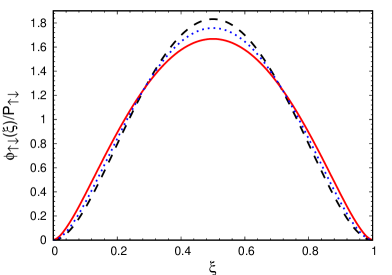
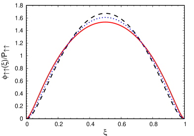
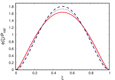
Figure 2: (color online) From top to bottom: anti-aligned, aligned, and total pion valence longitudinal-momentum distributions, normalized to 1, for three different sets of inputs parameters (cf. Table 1). Dashed line: set I. Dotted line: set IV. Solid line: set VIII, yielding the experimental value for $f_{\pi}$.

VI.2 The valence LF-momentum distributions

In this subsection, we present the dynamical quantities predicted for the pion on the null-plane: (i) the longitudinal-momentum distribution, $\phi(\xi)$, Eq. (27), and the transverse one, ${\cal P}(\gamma)$, Eq. (29), (ii) the valence LF-momentum density, ${\cal P}(\gamma,z)$, Eqs. (24), (25) and (26), (iii) the distribution amplitude, with its spin decomposition, and its transverse counterpart. The calculation of such quantities represents the needed first step, followed by the suitable evolution, for meaningful comparisons with experimental results, e.g., obtained in DIS and semi-inclusive DIS processes, like the pion parton distribution function and the transverse-momentum distributions, as well as extracted from the deeply-virtual Compton scattering, like the generalized parton distributions.

Let us first consider the longitudinal-momentum fraction distribution for the valence LF component, as a function of the quark longitudinal fraction $\xi$, and its anti-aligned and aligned components. It has to be stressed that on the null-plane, the longitudinal-momentum fraction distribution has the proper support, and therefore it fulfills both normalization and momentum sum rule when we take into account the whole set of the Fock components. This is a remarkable benefit for correctly analyzing DIS processes.

The calculations are shown in Fig. 2, for some illustrative cases, with the normalization equal to 1 (i.e. each distribution is divided by the respective probability) and the model parameters given in Table 1. Recall that the values for the gluon mass varies between 28 MeV $(\mu/m=0.15)$ and 638 MeV $(\mu/m=2.5)$, while the scale $\Lambda$ ranges between 255 MeV ($\Lambda/m=1$) to 430 MeV ($\Lambda/m=2$), covering a quite large interval of possibilities.

Figure 2 shows that the decrease of the effective dimensionless strength of the kernel, $\bar{\alpha}$, broadens $\phi(\xi)$ with a regular pattern, which is not too sensitive to the wide variations of both gluon mass and vertex parameter. Notice that even in presence of a very light gluon, the valence longitudinal distribution does not show dramatic changes, although they are visible. As expected, given its genuinely relativistic nature, the aligned distribution has a wider shape than the anti-aligned one, namely larger values of the quark momentum prevail, but the overall impact on the total distribution is mitigated by the smaller probability associated with the $S=1$ configuration. This observation is quantitatively corroborated by the analysis summarized in Table 2, where it is shown, for a few examples, the correlation between $\bar{\alpha}$ and the exponent of the function $(1-\xi)^{\eta}$, which we use, as customary, for fitting the valence longitudinal-momentum distributions close to the end-points.

Notice that the distributions are symmetric at the initial scale, while after evolving they cumulate at values $\xi\leq 0.5$ (as it will be discussed elsewhere). As pointed out in the previous subsection, the decreasing values of the valence probability and the corresponding increasing value of $\bar{\alpha}$ were put in relation with the increasing role of compact configurations, generated by higher Fock states. Plainly, also the increasing values of the exponent $\eta$ in the fitting functions can be explained through an analogous mechanism. In fact, the growth of the powers, shown in Table 2, depletes the valence quark distribution in the UV region, corresponding to $\xi\to 1$. The function $(1-\xi)^{\eta}$ becomes smaller and smaller for increasing values of $\eta$, and the probability of large longitudinal momenta decreases. This implies a suppression of configurations with the valence $q\bar{q}$ pair close together.

Table 2: An excerpt from the set of exponents of the fitting function $(1-\xi)^{\eta}$ for $\xi\to 1$, while varying the set of input parameters. The three columns, labeled by $\eta_{\uparrow\downarrow}$, $\eta_{\uparrow\uparrow}$ and $\eta$, correspond to the anti-aligned, aligned and total valence longitudinal-momentum distributions (cf. Fig. 2).

Set	${f_{\pi}}/m$	$\bar{\alpha}$	$\eta_{\uparrow\downarrow}$	$\eta_{\uparrow\uparrow}$	$\eta$
I	0.412	23.13	1.81	1.61	1.77
II	0.439	21.54	1.71	1.50	1.66
III	0.459	18.57	1.66	1.47	1.62
IV	0.478	18.16	1.61	1.42	1.57
VIII	0.510	11.21	1.44	1.26	1.40
IX	0.525	8.665	1.45	1.28	1.40

Table 3: An excerpt from the set of Mellin moments of the valence longitudinal momentum distribution, up to the sixth order. The contributions of the two spin configurations are also shown. N.B. The adopted normalization for the valence longitudinal-momentum distribution is equal to $P_{val}$.

Set	$\langle x\rangle$	$\langle x^{2}\rangle$	$\langle x^{3}\rangle$	$\langle x^{4}\rangle$	$\langle x^{5}\rangle$	$\langle x^{6}\rangle$
I	0.31	0.18	0.11	0.076	0.054	0.039
${\uparrow\downarrow}$	0.27	0.16	0.10	0.066	0.047	0.034
${\uparrow\uparrow}$	0.045	0.026	0.017	0.012	0.008	0.006
II	0.32	0.19	0.12	0.080	0.057	0.042
${\uparrow\downarrow}$	0.28	0.16	0.10	0.068	0.049	0.036
${\uparrow\uparrow}$	0.048	0.028	0.018	0.013	0.009	0.007
III	0.33	0.19	0.12	0.083	0.059	0.044
${\uparrow\downarrow}$	0.28	0.16	0.10	0.070	0.050	0.037
${\uparrow\uparrow}$	0.053	0.031	0.020	0.014	0.011	0.008
IV	0.33	0.19	0.12	0.082	0.059	0.043
${\uparrow\downarrow}$	0.28	0.16	0.10	0.070	0.050	0.037
${\uparrow\uparrow}$	0.053	0.031	0.020	0.014	0.010	0.008
VIII	0.35	0.20	0.13	0.091	0.066	0.049
${\uparrow\downarrow}$	0.28	0.17	0.11	0.074	0.054	0.040
${\uparrow\uparrow}$	0.068	0.041	0.027	0.019	0.014	0.011
IX	0.35	0.20	0.13	0.091	0.066	0.049
${\uparrow\downarrow}$	0.28	0.17	0.11	0.074	0.054	0.040
${\uparrow\uparrow}$	0.068	0.041	0.027	0.019	0.014	0.011

As already noticed, the aligned longitudinal-momentum distribution is broader than the anti-aligned one (cf. Fig. 2). This corresponds to a softer end-point behavior, with exponents systematically smaller than the anti-aligned ones, about $\eta^{\uparrow\downarrow}-\eta^{\uparrow\uparrow}\sim 0.2$, as shown in Table 2.

The results for the Mellin moments of the valence longitudinal-momentum distributions are shown in Table 3, also with the decomposition in spin contributions. It should be recalled that the present approach predicts a quite robust longitudinal fraction carried by the valence $q\bar{q}$ pair, according to $P_{val}$ that ranges from 60% to 70%. This can be assessed from the first Mellin moment, after noticing that if the valence $\phi(\xi)$ is normalized to 1, and not to $P_{val}$, the value of $\langle x\rangle$ is always 0.5, due to the symmetry of the valence wave function around $\xi=0.5$. It is interesting to observe that the moments do not change too much for the set of input parameters we have chosen, and the increasing values correspond to the increasing relevance of the momentum distribution close to the end-points. Such a behavior is clearly more evident for Mellin moments associated to higher powers. To carry out a detailed comparison with LQCD results and the analogous outcomes from the continuum QCD approach (see, e.g. Ref. Cloët and Roberts (2014)), one has to determine first the initial scale of the valence longitudinal-momentum distribution and then apply the evolution (see, e.g., Ref. de Paula et al. ).

The second dynamical quantity we have analyzed is the transverse-momentum distribution, $P(\gamma)$ (Eq. (29)), and its decomposition in spin configurations. The results, with normalization equal to $1$, are presented in Fig. 3 for the same set of parameters adopted for the longitudinal-momentum distribution in Fig. 2. The same general behavior found for the longitudinal-momentum distribution can be also recovered for the transverse-momentum one, namely, the size of the tail at large values of $\gamma$ becomes smaller for larger values of $\bar{\alpha}$, and vice-versa. As we learned, this is correlated to the role played by the typical size of the spatial correlation of the valence $q\bar{q}$ pair.

The anti-aligned and aligned distributions are also shown in Fig. 3. It is worth noticing that the last one has a slower decay compared to the anti-aligned case, since it carries a factor of $\gamma$, stemming from the relativistic spin-orbit coupling, which eventually adds a factor $\vec{k}_{\perp}$ to the momentum dependence of the aligned component in the valence wave function. The typical momentum scale that determines the effective strength, $\bar{\alpha}$, i.e. $\gamma/m^{2}\sim 0.2$, can be inferred from the behavior of $P(\gamma)/P(0)$ close to $\gamma=0$, as shown in Fig. 3. More explicitly, such value of $\gamma$ roughly indicates the region where $P(\gamma)$ is relevant for obtaining the actual value of the valence probability. Hence, the above mentioned range of $\gamma$ can be associated with the size of the region where the interaction is effective in building the $q\bar{q}$ bound state (in momentum space). In other words, such a low-energy or IR scale should govern the kernel of the BSE, so that it is effective in giving the strength necessary to create the strongly bound $q\bar{q}$ system, resulting in the pion.

Summarizing the first part of the analysis, one should point out that the end-point behavior of $\phi(\xi)$ is strongly correlated to the UV properties of the adopted kernel in the BSE, while the range of $\gamma$, where $P(\gamma)$ is large, is governed by the size of the bound state, i.e. by the IR behavior of the interaction.

An overall view of the pion in the 3D LF-momentum space can be obtained from Fig. 4, where the LF-momentum density ${\cal P}(\gamma,\xi)$ (cf. Eqs. (24), (25) and (26)), is shown. One should recall that the longitudinal and transverse distributions are obtained through the suitable integration of the density ${\cal P}(\gamma,\xi)$.

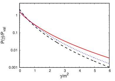
Figure 3: (color online) From top to bottom: anti-aligned, aligned and total pion valence transverse-momentum distributions, ${\cal P}(\gamma)$, normalized to 1, for three different sets of input parameters (cf. Table 1). Dashed line: set I. Dotted line: set IV. Solid line: set VIII, yielding the experimental value for $f_{\pi}$.

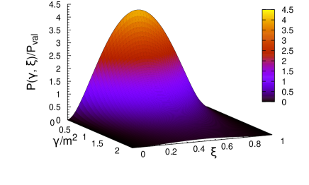
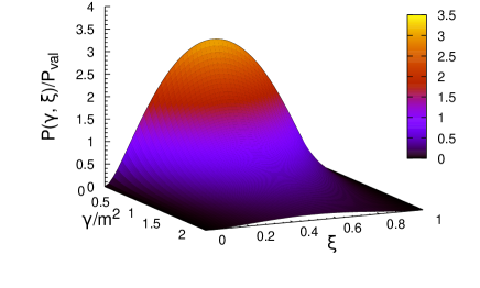
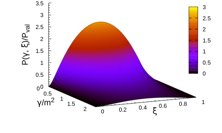
Figure 4: (color online) The LF-momentum density ${\cal P}(\gamma,\xi)$ (see Eqs. (24), (25) and (26)), vs $\xi$ and $\gamma=k^{2}_{\perp}$. From top to bottom: results for the parameter sets I, IV and VIII, respectively.

Finally, we show the distribution amplitude (DA) Lepage and Brodsky (1979); Efremov and Radyushkin (1980); Lepage and Brodsky (1980); Brodsky et al. (1998). This quantity is introduced through the factorization of the amplitudes associated with exclusive processes and can be expressed as an integral on the transverse-momentum dependence of the valence wave function. In particular, we have evaluated the following spin decompositions

$$\varphi_{\uparrow\downarrow}(\xi)=\frac{\int^{\infty}_{0}d\gamma~{}\psi_{\uparrow\downarrow}(\gamma,z)}{\int^{1}_{0}d\xi\int^{\infty}_{0}d\gamma~{}\psi_{\uparrow\downarrow}(\gamma,z)}\,,$$

$$\varphi_{\uparrow\uparrow}(\xi)=\frac{\int^{\infty}_{0}\,d\gamma~{}\psi_{\uparrow\uparrow}(\gamma,z)}{\int^{1}_{0}d\xi\int^{\infty}_{0}d\gamma~{}\psi_{\uparrow\uparrow}(\gamma,z)}\,.$$ (49)

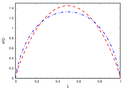
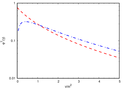
Figure 5: (color online) Pion distribution amplitude (upper panel) and the transverse one (lower panel) for the two spin components, obtained with the parameter set VIII. Dashed line: anti-aligned, $S=0$, component. Dash-dotted line: aligned, $S=1$, component.

Analogously, we have introduced the transverse distribution amplitude (TDA) by integrating the valence wave function over the fraction of longitudinal momentum carried by the valence quark (recall $z=1-2\xi$), viz

$$\varphi^{T}_{\uparrow\downarrow}(\gamma)=\frac{\int^{1}_{0}d\xi\,\psi_{\uparrow\downarrow}(\gamma,z)}{\int^{1}_{0}d\xi\int^{\infty}_{0}d\gamma\,\psi_{\uparrow\downarrow}(\gamma,z)}\,,$$

$$\varphi^{T}_{\uparrow\uparrow}(\gamma)=\frac{\int^{1}_{0}d\xi\,\psi_{\uparrow\uparrow}(\gamma,z)}{\int^{1}_{0}d\xi\int^{\infty}_{0}d\gamma\,\psi_{\uparrow\uparrow}(\gamma,z)}\,.$$ (50)

It has to be pointed out that the TDA is the Fourier transform of Eq. (42), namely the transverse amplitude in the transverse-coordinates space. The TDA can be also obtained from Euclidean-space calculations (see, e.g,. Ref. Gutierrez et al. (2016)).

The results for the two spin configurations of both DA and TDA, obtained by using the parameters of the set VIII, are shown in Fig. 5. It is interesting to observe that the aligned component of the DA is wider and decreases slower at the end-points than the anti-aligned component, as it happens for the longitudinal-momentum distributions (c.f. Table 2). The corresponding features can be recognized in the TDA case, where calculations are presented up to $\gamma/m^{2}\sim 5$ (about 0.3 GeV²) showing the characteristic IR scale of about $\gamma/m^{2}\sim 0.2$, implicitly carried by our input parameters. It should be recalled that while the UV region is governed by the one-gluon exchange, i.e. the short-range interaction, the IR region incorporates the features dictated by the long-range correlations in the transverse-coordinate space.

VI.3 The 3D image of the pion on the null-plane

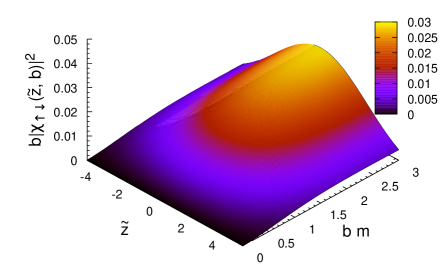
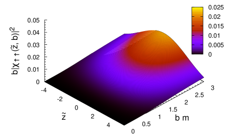
Figure 6: (color online) The pion in the 3D space $\{\tilde{z},{\bf b}\}$ (notice the rotational symmetry in the transverse plane) for the set VIII. Upper panel: anti-aligned component, $b\bigl{|}\chi_{\uparrow\downarrow}(\tilde{z},b)\bigr{|}^{2}$. Lower panel: aligned component, $b\bigl{|}\chi_{\uparrow\uparrow}(\tilde{z},b)\bigr{|}^{2}$. The variable $b\,m$ has been adopted for making the transverse coordinate adimensional.

In the 3D space described by the Ioffe-time and the transverse coordinates, one can obtain an image of the pion in terms of the two spin components of the valence wave function, i.e., $\chi_{\uparrow\downarrow(\uparrow\uparrow)}(\tilde{z},b)$, given in Eq. (39). Such a picture of the pion allows one to understand better the interplay between short and long light-like distances in the description of the hadron structure (see Sec. V). In view of this, one notices that the region with small values of $\{\tilde{z},{\bf b}\}$ is the place where the UV effects should manifest. Beside the 3D image, we also present the transverse amplitudes, $\tilde{\varphi}^{T}_{\uparrow\downarrow}(b)$ and $\tilde{\varphi}^{T}_{\uparrow\uparrow}(b)$, given in Eq. (42), since they could be the target of LQCD studies. To perform the calculations shown in this subsection, we have used the parameter set VIII (see Table 1) that fits the pion decay constant.

The 3D image of the pion spin components on the null-plane is provided in Fig. 6. Notice that the exponential factor ${\rm exp}(-\kappa\,b)$, present in the Fourier transform of $\varphi_{2}(\xi,{\bf k}_{\perp},\sigma_{i};M,J^{\pi},J_{z})$ (cf. Eqs. (93), (94) and (95)) is factorized out in both $\chi_{\uparrow\downarrow(\uparrow\uparrow)}(\tilde{z},b)$, allowing to use a linear scale in the 3D plot. For the purpose of the figure, each component is multiplied by the transverse coordinate $b$, canceling a log-type singularity at $b=0$, generated by the Bessel function $K_{0}$.

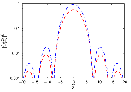
Figure 7: (color online) Squared integrated amplitudes $\bigl{|}\tilde{\Psi}_{\uparrow\uparrow(\uparrow\downarrow)}(\tilde{z})\bigr{|}^{2}$ (cf. Eq. (51)) vs the Ioffe-time, $\tilde{z}$, by using the parameter set VIII. Dashed line: anti-aligned component. Dash-dotted line: aligned component.

A general feature of both densities is the sharp enhancement for $\tilde{z}=0$, i.e., at vanishing light-like distances. Inspired by such an enhancement, and in order to better analyze the physically significant dependence upon $\tilde{z}$ of the valence wave function, we have also studied the absolute value squared of the integrals

$$\tilde{\Psi}_{\uparrow\downarrow(\uparrow\uparrow)}(\tilde{z})={\int_{0}^{\infty}{db\,b}~{}\tilde{\psi}_{\uparrow\downarrow(\uparrow\uparrow)}(\tilde{z},{b})\over\int_{0}^{\infty}{db\,b}\int_{-\infty}^{\infty}d\tilde{z}~{}\tilde{\psi}_{\uparrow\downarrow(\uparrow\uparrow)}(\tilde{z},{b})}\,,$$ (51)

with $\tilde{\psi}_{\uparrow\downarrow(\uparrow\uparrow)}(\tilde{z},{b})$ given in Eq. (V). These amplitudes have a more direct link to the spin components of the valence LF wave function since they also contain the original exponential factor ${\rm e}^{-\kappa\,b}$.

The integrated amplitudes in Eq. (51) describe each spin configuration where the constituents are at light-like distance $\tilde{z}$ and have relative transverse-momentum ${\bf k}_{\perp}=0$. As shown in Fig. 7, the amplitudes $\bigl{|}\tilde{\Psi}_{\uparrow\downarrow(\uparrow\uparrow)}(\tilde{z})\bigr{|}^{2}$, have a nice diffraction pattern, that represents a peculiar feature of such quantities, emphasizing the interference content due to the entangled $q\bar{q}$ pair.

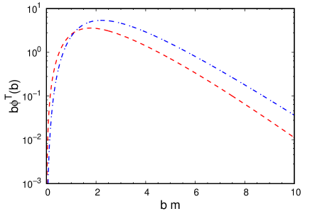
Figure 8: (color color) Transverse amplitudes for anti-aligned and aligned spin components of the pion valence wave function as a function $b\equiv|{\bf b}|$, for the parameter set VIII. Dashed line: anti-aligned component. Dash-dotted line: aligned component.

Finally, in Fig. 8, we present the Fourier transform of the transverse amplitudes, $\varphi^{T}_{\uparrow\downarrow(\uparrow\uparrow)}(\gamma)$ (Eq. (VI.2)), in the transverse-coordinate space, i.e.,

$$\phi^{T}_{\uparrow\uparrow(\uparrow\downarrow)}(b)={\int_{-\infty}^{\infty}d\tilde{z}~{}\tilde{\psi}_{\uparrow\downarrow(\uparrow\uparrow)}(\tilde{z},{b})\over\int_{0}^{\infty}{db\,b}\int_{-\infty}^{\infty}d\tilde{z}~{}\tilde{\psi}_{\uparrow\downarrow(\uparrow\uparrow)}(\tilde{z},{b})}\,.$$ (52)

The log-plot allows one to recognize the characteristic exponential decay at large distances, clearly dominated by $\exp(-\kappa b)$, which is the familiar fall-off of the wave function of a bound state ($\kappa^{2}=m^{2}-M^{2}/4>0$). Since the amplitudes depend upon transverse coordinates, they should be accessible to LQCD. Therefore, it could be interesting to compare its predictions with phenomenological calculations in order to get information about the highly nonlinear behavior of QCD at large transverse distances.

VII Conclusions and Perspectives

Within the light-front framework, where the physical intuition based on the Fock space expansion of the hadron wave function can be used at large extent, we have studied the strongly bound $q\bar{q}$ system that generates the pion. In our approach, the Bethe-Salpeter equation in Minkowski space is solved by using the Nakanishi integral representation of the BS amplitude. The ladder approximation of the BS interaction kernel in the Feynman gauge has been considered, with the constituent quarks interacting by an effective massive gluon exchange. An extended effective quark-gluon vertex function is introduced through a form factor, that contains a new scale parameter, beside the gluon mass. The range where (i) the form-factor parameter $\Lambda$, (ii) the quark effective mass and (iii) the gluon one can vary has been chosen according to LQCD results, with the guideline given by the value of the IR scale $\Lambda_{QCD}$. We fine-tuned the parameters around such a scale in order to reproduce $f_{\pi}$. Once the BSE has been solved, we formally obtained the valence LF wave function, that is well-defined in terms of the lowest number of fields associated to the BS amplitude, and therefore it contains unambiguous information on the dynamics that one can convey into the interaction kernel of the BSE itself.

The detailed study of the valence Fock component has been carried out by first addressing static (or integral) quantities, like: (i) the pion decay constant, $f_{\pi}$, and (ii) the valence probability, whose value is around $70\%$, according to our calculations. A relevant and peculiar feature of our approach is the possibility of decomposing the valence component in the two allowed spin configuration: the dominant $S=0$ component and the purely relativistic $S=1$, that yields a $\sim 20\%$ contribution to the valence probability. Such a decomposition also has been applied to the second set of investigated quantities, bringing a considerable wealth of dynamical information. In particular, we have analyzed: (i) the longitudinal and transverse LF-momentum distributions; (ii) the distribution amplitudes that depend upon the longitudinal and transverse LF-momentum components; (iii) the probability densities in momentum and configuration spaces (the last one is given by the Cartesian product of the covariant Ioffe-time and the Euclidean transverse coordinates). For each quantity, we have highlighted signatures of the dynamics governed by the one-gluon exchange and have also emphasized the relevance of the transverse degrees of freedom, more accessible to the LQCD studies.

Future developments of our approach are primarily related to the implementation of both quark and gluon dressed propagators, more realistic dressed quark-gluon vertex, in order to extend to the Minkowski space the successful studies of the spontaneously broken chiral symmetry performed in the Euclidean space. In this way, the kernel of the BSE can be improved systematically, adding step by step new dynamical contents from QCD, that one should explore in the elaboration of hadron models. Furthermore, observables like the electromagnetic form factor and generalized transverse-momentum dependent parton distributions (see, e.g., Ref.Lorcé et al. (2011)) of the pion are within our plans for future studies.

Appendix A The valence wave function and the valence probability

In this Appendix, the valence probability is decomposed into the contributions generated by the spin configurations active inside the pion.

Let us first illustrate the relation between the BS amplitude and the valence wave function, i.e. the amplitude with the lowest number of constituents in the Fock expansion of the bound system. Recalling the key observation contained in Ref. Chang and Yan (1973), i.e. the independent degrees of freedom described by the fermionic field on the null-plane is given by the projections $\psi^{(+)}(\tilde{x},x^{+}=0^{+})=\Lambda^{+}\psi(\tilde{x},x^{+}=0^{+})$ with $\tilde{x}\equiv\{x^{-},{\bf x}_{\perp}\}$ and

$$\Lambda^{\pm}={1\over 4}\gamma^{\mp}\gamma^{\pm}~{}~{},\quad\Lambda^{\pm}\Lambda^{\pm}=\Lambda^{\pm}~{}~{},\quad\Lambda^{+}+\Lambda^{-}=1~{}~{},$$

$$~{}\Lambda^{\pm}\gamma^{0}\Lambda^{\pm}=0~{}~{},\quad\Lambda^{\pm}\gamma^{0}\Lambda^{\mp}={\gamma^{\mp}\over 2}~{}~{},\quad Tr\Bigl{\{}\Lambda^{\pm}\Bigr{\}}=2~{}~{}.$$

one can write the good component of the fermion field as follows

$$\psi^{(+)}(\tilde{x},x^{+}=0^{+})=\int{d\tilde{q}\over(2\pi)^{3/2}}~{}{\theta(q^{+})\over\sqrt{2q^{+}}}~{}\sum_{\sigma}$$

$$\Bigl{[}U^{(+)}(\tilde{q},\sigma)~{}b(\tilde{q},\sigma)e^{i\tilde{q}\cdot\tilde{x}}+V^{(+)}(\tilde{q},\sigma)~{}d^{\dagger}(\tilde{q},\sigma)e^{-i\tilde{q}\cdot\tilde{x}}\Bigr{]}~{},$$

where

$$U^{(+)}(\tilde{q},\sigma)=\Lambda^{+}u(\tilde{q},\sigma)~{}~{},\quad V^{(+)}(\tilde{q},\sigma)=\Lambda^{+}v(\tilde{q},\sigma)~{},$$

with the normalization $\bar{u}~{}u=2m$ and $\bar{v}(\tilde{q},\sigma^{\prime})v(\tilde{q},\sigma)=-2m$. Hence, one expresses the fermion creation and annihilation operators associated with $b$ and $d$, in terms of the good component of the field, as follows

$$(2\pi)^{3/2}~{}\theta(q^{+})~{}\sqrt{2q^{+}}~{}b(\tilde{q},\sigma^{\prime})=$$

$$=\int d\tilde{x}~{}e^{-i\tilde{q}\cdot\tilde{x}}~{}U^{(+)\dagger}(\tilde{q},\sigma^{\prime})\psi^{(+)}(\tilde{x},x^{+}=0^{+})~{}~{},$$

$$(2\pi)^{3/2}~{}\theta(q^{+})~{}\sqrt{2q^{+}}~{}d^{\dagger}(\tilde{q},\sigma^{\prime})=$$

$$=\int d\tilde{x}~{}e^{i\tilde{q}\cdot\tilde{x}}~{}V^{(+)\dagger}(\tilde{q},\sigma^{\prime})\psi^{(+)}(\tilde{x},x^{+}=0^{+})~{}~{},$$ (56)

where

$$u^{\dagger}(\tilde{q},\sigma^{\prime})\Lambda^{+}u(\tilde{q},\sigma)=q^{+}\delta_{\sigma^{\prime},\sigma}~{}~{},$$

$$v^{\dagger}(\tilde{q},\sigma^{\prime})\Lambda^{+}v(\tilde{q},\sigma)=q^{+}\delta_{\sigma,\sigma^{\prime}}~{}~{}.$$ (57)

Once the creation and annihilation operators for the fermions are defined, one can construct the Fock component with the lowest number of constituents and therefore introduce the LF valence amplitude, $\varphi_{2}(\xi,\bm{k}_{\perp},\sigma_{i};M,J^{\pi},J_{z})$. It reads

$$\varphi_{2}(\xi,\bm{k}_{\perp},\sigma_{i};M,J^{\pi},J_{z})=(2\pi)^{3}~{}\sqrt{N_{c}}~{}2p^{+}\sqrt{\xi(1-\xi)}$$

$$\times~{}\langle 0|b(\tilde{q}_{2},\sigma_{2})~{}d(\tilde{q}_{1},\sigma_{1})|\tilde{p},M,J^{\pi},J_{z}\rangle~{},$$ (58)

where $\tilde{q}_{1}\equiv\{q^{+}_{1}=M(1-\xi),-{\bf k}_{\perp}\}$, $\tilde{q}_{2}\equiv\{q_{2}^{+}=M\xi,{\bf k}_{\perp}\}$ and $\xi=1/2+k^{+}/p^{+}$.

From the general expression of the BS amplitude (cf. Eq. (1), adapted to the general notation of this Appendix) and Eq. (58), one can show that the valence amplitude is related to the BS one by

$$\varphi_{2}(\xi,\bm{k}_{\perp},\sigma_{i};M,J^{\pi},J_{z})={\sqrt{N_{c}}\over p^{+}}{1\over 4}~{}\bar{u}_{\alpha}(\tilde{q}_{2},\sigma_{2})$$

$$\times~{}\int{dk^{-}\over 2\pi}\Bigl{[}\gamma^{+}~{}\Phi(k,p)\,\gamma^{+}\Bigr{]}_{\alpha\beta}~{}v_{\beta}(\tilde{q}_{1},\sigma_{1})~{}~{}.$$ (59)

More explicitly, from Eqs. (7) and (8) one gets

$$\varphi_{2}(\xi,\bm{k}_{\perp},\sigma_{i};M,J^{\pi},J_{z})={\sqrt{N_{c}}\over p^{+}}{1\over 4}~{}\bar{u}(\tilde{q}_{2},\sigma_{2})~{}\int{dk^{-}\over 2\pi}$$

$$\times~{}\gamma^{+}~{}~{}\Biggl{[}{/\!\!\!p\over M}~{}\phi_{2}+\Bigl{(}{k\cdot p\over M^{3}}/\!\!\!p-{/\!\!\!k\over M}\Bigr{)}~{}\phi_{3}-{1\over M^{2}}/\!\!\!p~{}/\!\!\!k~{}\phi_{4}\Biggr{]}~{}\gamma_{5}$$

$$\times~{}\gamma^{+}~{}v(\tilde{q}_{1},\sigma_{1})=$$

$$=-~{}{\sqrt{N_{c}}\over p^{+}}~{}\int{dk^{-}\over 2\pi}~{}\Biggl{\{}\Biggl{[}\phi_{2}+\Bigl{(}{k^{-}\over 2M}+{z\over 4}\Bigr{)}~{}\phi_{3}\Biggr{]}$$

$$\times~{}D_{1}^{\sigma_{1}\sigma_{2}}(\tilde{q}_{1},\tilde{q}_{2})-{1\over M}~{}D_{2}^{\sigma_{1}\sigma_{2}}(\tilde{q}_{1},\tilde{q}_{2})~{}\phi_{4}\Biggr{\}}~{}~{},$$ (60)

where the following relations have been exploited: $\gamma^{\pm}\gamma^{\pm}=0$, $\gamma^{-}~{}\gamma^{+}~{}\gamma^{-}=4\gamma^{-}$ (and the analogous for the other combination). Moreover,

$$D_{1}^{\sigma_{1}\sigma_{2}}(\tilde{q}_{1},\tilde{q}_{2})=~{}Tr\Bigl{\{}{\cal P}^{\sigma_{1}\sigma_{2}}(\tilde{q}_{1},\tilde{q}_{2})~{}\gamma_{5}~{}\Lambda^{+}\Bigr{\}}$$

$$D_{2}^{\sigma_{1}\sigma_{2}}(\tilde{q}_{1},\tilde{q}_{2})=~{}Tr\Bigl{\{}{\cal P}^{\sigma_{1}\sigma_{2}}(\tilde{q}_{1},\tilde{q}_{2})~{}{\bf k}_{\perp}\cdot{\bm{\gamma}}_{\perp}~{}\gamma_{5}~{}\Lambda^{+}\Bigr{\}}~{},$$

(61)

with

$${\cal P}^{\sigma_{1}\sigma_{2}}(\tilde{q}_{1},\tilde{q}_{2})=v(\tilde{q}_{1},\sigma_{1})u^{\dagger}(\tilde{q}_{2},\sigma_{2})~{}~{}.$$ (62)

The spinors $u$ and $v$ in terms of the LF variables can be found in Appendix B of Ref. Brodsky et al. (1998), namely

$$u(\tilde{q},\sigma)={q^{+}+\gamma^{0}~{}m+\gamma^{0}{\bf q}_{\perp}\cdot{\bm{\gamma}}_{\perp}\over\sqrt{2q^{+}}}~{}\begin{pmatrix}\chi^{\sigma}\\ \sigma\chi^{\sigma}\end{pmatrix}$$ (63)

and

$$v(\tilde{q},-\sigma)={q^{+}-\gamma^{0}~{}m+\gamma^{0}{\bf q}_{\perp}\cdot{\bm{\gamma}}_{\perp}\over\sqrt{2q^{+}}}~{}\left(\begin{array}[]{c}\chi^{\sigma}\\ \sigma\chi^{\sigma}\end{array}\right)~{}~{},$$ (66)

with $\sigma=\pm 1$. Notice that in $v$ there is an opposite sign for the helicity (in the LF framework helicity and third component of the spin coincide, see, e.g., Chiu and Brodsky (2017)). For a quick evaluation of the above matrix elements in Eqs. (61), it is useful to introduce the following dyadic products

$$\begin{pmatrix}\chi^{\sigma}\\ \sigma\chi^{\sigma}\end{pmatrix}\begin{array}[]{c}\begin{pmatrix}\chi^{\sigma\dagger}&\sigma\chi^{\sigma\dagger}\end{pmatrix}\\ {}\hfil\end{array}=(1+\sigma\gamma_{5})~{}\Lambda^{+}~{}~{},$$ (70)

$$\begin{pmatrix}\chi^{-\sigma}\\ -\sigma\chi^{-\sigma}\end{pmatrix}\begin{array}[]{c}\begin{pmatrix}\chi^{\sigma\dagger}&\sigma\chi^{\sigma\dagger}\end{pmatrix}\\ {}\hfil\end{array}=(1-\sigma\gamma_{5})~{}{\gamma_{L(R)}\over\sqrt{2}}~{}~{},$$ (73)

(74)

where in Eq. (74) for $\sigma=\pm 1$ one has to use $\gamma_{L(R)}$, with

$$\gamma_{R(L)}=\mp~{}{1\over\sqrt{2}}(\gamma^{1}\pm i\gamma^{2})~{}~{}.$$ (75)

The actual expressions of $D_{1}$ and $D_{2}$ can be obtained through suitable traces. In particular, for $D_{1}^{-\sigma\sigma}$ one gets

$$D_{1}^{-\sigma\sigma}(\tilde{q}_{1},\tilde{q}_{2})=Tr\Bigl{\{}{q^{+}_{1}-\gamma^{0}~{}m{-}\gamma^{0}{\bf k}_{\perp}\cdot{\bm{\gamma}}_{\perp}\over\sqrt{2q^{+}_{1}}}$$

$$\times~{}(1+\sigma\gamma_{5})\Lambda^{+}~{}{q^{+}_{2}+\gamma^{0}~{}m{+}\gamma^{0}{\bf k}_{\perp}\cdot{\bm{\gamma}}_{\perp}\over\sqrt{2q^{+}_{2}}}~{}\gamma_{5}~{}\Lambda^{+}\Bigr{\}}=$$

$$={\sqrt{q^{+}_{1}q^{+}_{2}}\over 2}~{}Tr\Bigl{\{}(1+\sigma\gamma_{5})~{}\Lambda^{+}~{}~{}\gamma_{5}~{}\Lambda^{+}\Bigr{\}}=$$

$$=\sigma~{}{M}\sqrt{\xi(1-\xi)}=\sigma~{}{M\over 2}\sqrt{1-z^{2}}~{}~{},$$ (76)

where we can properly move the projector $\Lambda^{+}$ inside the trace for simplifying the whole expression, e.g.

$$\Lambda^{+}~{}[q^{+}_{1}-\gamma^{0}~{}m-\gamma^{0}{\bf k}_{\perp}\cdot{\bm{\gamma}}_{\perp}]\Lambda^{+}=\Lambda^{+}~{}q^{+}_{1}$$

$$\Lambda^{+}~{}[q^{+}_{2}+\gamma^{0}~{}m+\gamma^{0}{\bf k}_{\perp}\cdot{\bm{\gamma}}_{\perp}]\Lambda^{+}=\Lambda^{+}~{}q^{+}_{2}~{}.$$ (77)

By using the previous relations, one can show that the matrix $D_{2}^{-\sigma\sigma}$ vanishes, viz.

$$D_{2}^{-\sigma\sigma}(\tilde{q}_{1},\tilde{q}_{2})=Tr\Bigl{\{}{q^{+}_{1}-\gamma^{0}~{}m{-}\gamma^{0}{\bf k}_{\perp}\cdot{\bm{\gamma}}_{\perp}\over\sqrt{2q^{+}_{1}}}$$

$$\times~{}(1+\sigma\gamma_{5})~{}\Lambda^{+}~{}{q^{+}_{2}+\gamma^{0}~{}m{+}\gamma^{0}{\bf k}_{\perp}\cdot{\bm{\gamma}}_{\perp}\over\sqrt{2q^{+}_{2}}}$$

$$\times~{}{\bf q}_{\perp}\cdot{\bm{\gamma}}_{\perp}~{}\gamma_{5}~{}\Lambda^{+}\Bigr{\}}=0~{}~{}.$$ (78)

Also $D_{1}^{\sigma\sigma}$ is vanishing, once the following relation is adopted

$$\gamma_{5}~{}[q^{+}_{2}-\gamma^{0}~{}m+\gamma^{0}{\bf k}_{\perp}\cdot{\bm{\gamma}}_{\perp}]\Lambda^{+}$$

$$\times~{}[q^{+}_{1}-\gamma^{0}~{}m-\gamma^{0}{\bf k}_{\perp}\cdot{\bm{\gamma}}_{\perp}]=$$

$$=\gamma_{5}~{}q^{+}_{2}[q^{+}_{1}\Lambda^{+}-{\gamma^{-}\over 2}~{}m-{\gamma^{-}\over 2}{\bf k}_{\perp}\cdot{\bm{\gamma}}_{\perp}]$$

$$-\gamma_{5}~{}{m\over 2}[q^{+}_{1}\gamma^{+}-\gamma^{+}{\gamma^{-}\over 2}~{}m]$$

$$+\gamma_{5}~{}{1\over 2}{\bf k}_{\perp}\cdot{\bm{\gamma}}_{\perp}[q^{+}_{1}\gamma^{+}-\gamma^{+}{\gamma^{-}\over 2}{\bf k}_{\perp}\cdot{\bm{\gamma}}_{\perp}]~{},$$ (79)

and the standard results for the traces of the Dirac matrixes. Namely, one gets

$$D_{1}^{\sigma\sigma}(\tilde{q}_{1},\tilde{q}_{2})=Tr\Bigl{\{}{q^{+}_{1}-\gamma^{0}~{}m{-}\gamma^{0}{\bf k}_{\perp}\cdot{\bm{\gamma}}_{\perp}\over\sqrt{2q^{+}_{1}}}$$

$$\times~{}(1-\sigma\gamma_{5}){\gamma_{L(R)}\over\sqrt{2}}~{}~{}{q^{+}_{2}+\gamma^{0}~{}m{+}\gamma^{0}{\bf k}_{\perp}\cdot{\bm{\gamma}}_{\perp}\over\sqrt{2q^{+}_{2}}}$$

$$\times~{}\gamma_{5}~{}\Lambda^{+}\Bigr{\}}=0~{}~{}.$$ (80)

The last matrix element $D_{2}^{\sigma\sigma}$ is given by

$$D_{2}^{\sigma\sigma}(\tilde{q}_{1},\tilde{q}_{2})=Tr\Bigl{\{}{q^{+}_{1}-\gamma^{0}~{}m{-}\gamma^{0}{\bf k}_{\perp}\cdot{\bm{\gamma}}_{\perp}\over\sqrt{2q^{+}_{1}}}$$

$$\times~{}(1-\sigma\gamma_{5})~{}{\gamma_{L(R)}\over\sqrt{2}}~{}{(q^{+}_{2}+\gamma^{0}~{}m){\bf k}_{\perp}\cdot{\bm{\gamma}}_{\perp}{+}\gamma^{0}|{\bf k}_{\perp}|^{2}\over\sqrt{2q^{+}_{2}}}$$

$$\times~{}\gamma_{5}~{}\Lambda^{+}\Bigr{\}}=-{\sqrt{q^{+}_{1}q^{+}_{2}}\over 2\sqrt{2}}$$

$$\times~{}Tr\Bigl{\{}(1-\sigma\gamma_{5})~{}\gamma_{L(R)}~{}\Bigl{(}k_{R}\gamma_{L}+k_{L}\gamma_{R}\Bigr{)}~{}\gamma_{5}\Lambda^{+}\Bigr{\}}=$$

$$=\sigma~{}k_{L(R)}M~{}\sqrt{(1-z^{2})\over 2}~{}~{},$$ (81)

where

$$k_{R(L)}=\mp~{}{1\over\sqrt{2}}(k_{x}\pm ik_{y})~{}~{},$$ (82)

and the following relations have been used

$$\gamma_{R(L)}\gamma_{R(L)}=0~{}~{},$$

$${1\over 4}Tr\Bigl{\{}(\gamma_{5}-\sigma)~{}\gamma^{-}\gamma^{+}\gamma_{L(R)}\gamma_{R(L)}\Bigr{\}}=$$

$$={1\over 2}Tr\Bigl{\{}(\gamma_{5}-\sigma)~{}(1+\gamma^{0}\gamma^{3})~{}(1-\sigma~{}\sigma^{12})\Bigr{\}}=$$

$$=-2\sigma-2\sigma~{}{1\over 4}Tr\Bigl{\{}\gamma_{5}~{}\gamma^{0}\gamma^{3}~{}i\gamma^{1}\gamma^{2}\Bigr{\}}=$$

$$=-4\sigma~{}~{},$$ (83)

recalling that for $\sigma=\pm 1$ one has the product $\gamma_{L(R)}~{}\gamma_{R(L)}$. Finally, by inserting the above results into Eq. (60), one gets

$$\varphi_{2}(\xi,\bm{k}_{\perp},\sigma_{i};M,J^{\pi},J_{z})=~{}-{\sigma_{2}\over 2}~{}\sqrt{N_{c}}~{}\sqrt{1-z^{2}}$$

$$\times~{}\int{dk^{-}\over 2\pi}\Biggl{\{}\delta_{\sigma_{2},-\sigma_{1}}\Biggl{(}\phi_{2}(k,p)+\Bigl{(}{k^{-}\over 2M}+{z\over 4}\Bigr{)}\phi_{3}(k,p)\Biggr{)}$$

$${{-}}{k_{L(R)}\sqrt{2}\over M}~{}\delta_{\sigma_{2},\sigma_{1}}~{}\phi_{4}(k,p)\Biggr{\}}~{}~{}.$$ (84)

The integration over $k^{-}$ can be readily performed by using the NIR of the scalar functions $\phi_{i}$, Eq. (9). Explicitly, one gets (cf Refs. de Paula et al. (2016, 2017))

$${{\psi_{i}(\gamma,\xi)}}=-{i\over M}~{}\int_{0}^{\infty}d\gamma^{\prime}$$

$$\times~{}{g_{i}(\gamma^{\prime},z;\kappa^{2})\over[\gamma^{\prime}+\gamma+m^{2}z^{2}+(1-z^{2})\kappa^{2}-i\epsilon]^{2}}~{}~{},$$ (85)

with $z=1-2\xi$. Hence, one can write

$$\varphi_{2}(\xi,\bm{k}_{\perp},\sigma_{i};M,J^{\pi},J_{z})=~{}-{\sigma_{2}\over 2}~{}\sqrt{N_{c}}~{}\sqrt{1-z^{2}}$$

$$\times~{}\Biggl{\{}\delta_{\sigma_{2},-\sigma_{1}}\Biggl{[}\psi_{2}(\gamma,z)+{z\over 2}{{\psi_{3}(\gamma,z)}}$$

$$+{i\over M^{3}}~{}\int_{0}^{\infty}d\gamma^{\prime}~{}~{}{\partial g_{3}(\gamma^{\prime},z;\kappa^{2})/\partial z\over\gamma+\gamma^{\prime}+z^{2}m^{2}+(1-z^{2})\kappa^{2}-i\epsilon}~{}\Biggr{]}$$

$$~{}-~{}{k_{L(R)}\sqrt{2}\over M}~{}\delta_{\sigma_{2},\sigma_{1}}~{}\psi_{4}(\gamma,z)\Biggr{\}}~{}~{},$$ (86)

where for $\sigma_{2}=\sigma_{1}=\pm 1$ one has to use $k_{L(R)}$. From Refs. de Paula et al. (2016, 2017), the cumbersome term $k^{-}~{}\phi_{3}$ contains a LF singularity, can be manipulated as follows

$$\int{dk^{-}\over 2\pi}~{}k^{-}~{}\phi_{3}(k,p)=$$

$$=\int_{-1}^{+1}dz^{\prime}\int_{0}^{\infty}d\gamma^{\prime}g_{3}(\gamma^{\prime},z^{\prime};\kappa^{2})~{}{\cal I}_{1}(\gamma^{\prime},z^{\prime},z)~{}~{},$$ (87)

where

$${\cal I}_{1}(\gamma^{\prime},z^{\prime},z)=\int{dk^{-}\over 2\pi}$$

$$\times~{}{k^{-}\over[k^{-}(z^{\prime}-z){M\over 2}-zz^{\prime}{M^{2}\over 4}-\gamma-\gamma^{\prime}-\kappa^{2}+i\epsilon]^{3}}~{},$$

with $z=-2k^{+}/M$. N.B. the integral ${\cal I}_{1}$ becomes singular for $z^{\prime}=z$. Its evaluation proceeds by using (see also Ref. Yan (1973))

$$\int_{-\infty}^{\infty}{dx\over 2\pi}~{}{1\over\Bigl{[}\beta~{}x-y\mp i\epsilon\Bigr{]}^{n}}=~{}\pm{i\over n-1}~{}{\delta(\beta)\over\Bigl{[}-y\mp i\epsilon\Bigr{]}^{n-1}}~{}~{}.$$

Thus, one gets

$${\cal I}_{1}(\gamma^{\prime},z^{\prime},z)=-~{}i{2\over M^{2}}{\delta(z^{\prime}-z)\over(z^{\prime}-z)}$$

$$\times~{}{1\over\left[-zz^{\prime}M^{2}/4-\gamma-\gamma^{\prime}-\kappa^{2}+i\epsilon\right]}=$$

$$=i~{}\delta^{\prime}(z^{\prime}-z)~{}{2\over M^{2}}~{}{1\over\left[-zz^{\prime}M^{2}/4-\gamma-\gamma^{\prime}-\kappa^{2}+i\epsilon\right]}~{},$$

where the derivative of the delta function fulfills the relation: $x~{}\delta^{\prime}(x)=-\delta(x)$, since $d[x~{}\delta(x)]/dx=0$. By inserting this result into Eq. (87), and properly integrating by parts, one gets

$$\int{dk^{-}\over 2\pi}~{}{k^{-}\over 2M}~{}\phi_{3}(k,p)=$$

$$={i\over M^{3}}~{}\int_{0}^{\infty}d\gamma^{\prime}~{}~{}{\partial g_{3}(\gamma^{\prime},z;\kappa^{2})/\partial z\over\left[\gamma+\gamma^{\prime}+z^{2}m^{2}+(1-z^{2})\kappa^{2}-i\epsilon\right]}$$

$$+{z\over 4}~{}\psi_{3}(\gamma,\xi){\color[rgb]{0,0,1}.}$$ (91)

Appendix B Orbital angular momentum decomposition on the transverse-plane

In this Appendix we illustrate some formal steps for obtaining the Fourier transform of the the two spin components of the valence wave function $\varphi_{2}$ (cf. Eq. (19)), as given in Eq. (V). As a by-product, the obtained results allow one to emphasize the $L_{z}$ content in each contribution (recall that $L_{z}=xp_{y}-yp_{x}$, and it is a kinematical generator, within the LF framework).

Let us first recall that

$${\rm e}^{{i}x\cos\theta}=\sum_{m=-\infty}^{m=\infty}{i}^{m}J_{m}(x){\rm e}^{{i}m\,\theta}\,,$$ (92)

where $J_{m}(x)$ is the Bessel function of integer order. In particular, the Fourier transform of the spin anti-aligned and aligned components are associated with integrals of $J_{0}$ and $J_{1}$ respectively, after performing the angular integration in Eq. (V).

By adopting the expression of $\psi_{\uparrow\downarrow}(\gamma,z)$ and $\psi_{\uparrow\downarrow}(\gamma,z)$ in terms of the respective NIRs (cf. Eqs. (III) and (21)), one has to evaluate the following integrals. The first one is

$$F_{0}(z,\gamma^{\prime},b)=\int^{\infty}_{0}d\gamma~{}{J_{0}(b\sqrt{\gamma})\over\gamma+\gamma^{\prime}+\kappa^{2}+z^{2}\tfrac{M^{2}}{4}}\\ =2K_{0}\left(b\,\sqrt{\gamma^{\prime}+\kappa^{2}+z^{2}\tfrac{M^{2}}{4}}\right)\,,$$ (93)

where $K_{n}(x)$ is the modified Bessel function of the second kind. The other two integrals are

$$F^{\prime}_{0}(z,\gamma^{\prime},b)=\int^{\infty}_{0}d\gamma~{}{J_{0}(b\sqrt{\gamma})\over(\gamma+\gamma^{\prime}+\kappa^{2}+z^{2}\frac{M^{2}}{4})^{2}}\\ =\frac{b\,K_{1}\left(b\,\sqrt{\gamma^{\prime}+\kappa^{2}+z^{2}\tfrac{M^{2}}{4}}\right)}{\sqrt{\gamma^{\prime}+\kappa^{2}+z^{2}\tfrac{M^{2}}{4}}}\,,$$ (94)

and

$$F_{1}(z,\gamma^{\prime},b)=\int^{\infty}_{0}d\gamma~{}{\sqrt{\gamma}J_{1}(b\sqrt{\gamma})\over[\gamma+\gamma^{\prime}+\kappa^{2}+z^{2}\tfrac{M^{2}}{4}]^{2}}\\ =bK_{0}\left(b\,\sqrt{\gamma^{\prime}+\kappa^{2}+z^{2}\tfrac{M^{2}}{4}}\right)\,.$$ (95)

Notice that $F_{0}$, $F^{\prime}_{0}$ and $F_{1}$ depend upon $z^{2}$, and this allows one to eliminate odd functions when integrating on $z$ in Eq. (V). The driving exponential fall-off of $F_{0}$, $F_{0}^{\prime}$ and $F_{1}$ in the asymptotic limit $b\rightarrow\infty$ comes from $K_{m}(x)$, which reads:

$$K_{m}(x)|_{x\to\infty}\to\left(\frac{\pi}{2\,x}\right)^{\frac{1}{2}}{\rm e}^{-x}~{}~{}.$$ (96)

Hence, the leading exponential behavior in the integrals (93), (94) and (95) comes from values of ${\rm e}^{-b\,\sqrt{\gamma^{\prime}+\kappa^{2}+z^{2}\tfrac{M^{2}}{4}}}$ (as seen from Eq. (96)) with $\gamma^{\prime}$ close to $0$ and $z\sim 0$, namely

$$F_{0}(z\sim 0,\gamma^{\prime}\sim 0,b)|_{b\to\infty}=$$

$$=b^{-1/2}F^{\prime}_{0}((z\sim 0,\gamma^{\prime}\sim 0,b)|_{b\to\infty}=$$

$$=b^{-1}F_{1}((z\sim 0,\gamma^{\prime}\sim 0,b)|_{b\to\infty}\sim~{}{\rm e}^{-b\,\kappa}~{}~{},$$ (97)

with $\kappa$ given in Eq. (10).

References

- Aguilar et al. (2019) Arlene C. Aguilar et al., “Pion and Kaon Structure at the Electron-Ion Collider,” Eur. Phys. J. A 55, 190 (2019), arXiv:1907.08218 [nucl-ex] .
- Barry et al. (2018) P.C. Barry, N. Sato, W. Melnitchouk, and Chueng-Ryong Ji, “First Monte Carlo Global QCD Analysis of Pion Parton Distributions,” Phys. Rev. Lett. 121, 152001 (2018), arXiv:1804.01965 [hep-ph] .
- Shi and Cloët (2019) Chao Shi and Ian C. Cloët, “Intrinsic Transverse Motion of the Pion’s Valence Quarks,” Phys. Rev. Lett. 122, 082301 (2019), arXiv:1806.04799 [nucl-th] .
- Bednar et al. (2020) Kyle D. Bednar, Ian C. Cloët, and Peter C. Tandy, “Distinguishing Quarks and Gluons in Pion and Kaon Parton Distribution Functions,” Phys. Rev. Lett. 124, 042002 (2020), arXiv:1811.12310 [nucl-th] .
- Oehm et al. (2019) M. Oehm, C. Alexandrou, M. Constantinou, K. Jansen, G. Koutsou, B. Kostrzewa, F. Steffens, C. Urbach, and S. Zafeiropoulos, “ and of the pion PDF from lattice QCD with dynamical quark flavors,” Phys. Rev. D 99, 014508 (2019), arXiv:1810.09743 [hep-lat] .
- Lan et al. (2019) Jiangshan Lan, Chandan Mondal, Shaoyang Jia, Xingbo Zhao, and James P. Vary, “Parton Distribution Functions from a Light Front Hamiltonian and QCD Evolution for Light Mesons,” Phys. Rev. Lett. 122, 172001 (2019), arXiv:1901.11430 [nucl-th] .
- Lan et al. (2020) Jiangshan Lan, Chandan Mondal, Shaoyang Jia, Xingbo Zhao, and James P. Vary, “Pion and kaon parton distribution functions from basis light front quantization and QCD evolution,” Phys. Rev. D 101, 034024 (2020), arXiv:1907.01509 [nucl-th] .
- Ding et al. (2020a) Minghui Ding, Khépani Raya, Daniele Binosi, Lei Chang, Craig D Roberts, and Sebastian M. Schmidt, “Symmetry, symmetry breaking, and pion parton distributions,” Phys. Rev. D 101, 054014 (2020a), arXiv:1905.05208 [nucl-th] .
- Ding et al. (2020b) Minghui Ding, Khépani Raya, Daniele Binosi, Lei Chang, Craig D Roberts, and Sebastian M Schmidt, “Drawing insights from pion parton distributions,” Chin. Phys. C 44, 031002 (2020b), arXiv:1912.07529 [hep-ph] .
- Sufian et al. (2020) Raza Sabbir Sufian, Colin Egerer, Joseph Karpie, Robert G. Edwards, Bálint Joó, Yan-Qing Ma, Kostas Orginos, Jian-Wei Qiu, and David G. Richards, “Pion Valence Quark Distribution from Current-Current Correlation in Lattice QCD,” Phys. Rev. D 102, 054508 (2020), arXiv:2001.04960 [hep-lat] .
- Chang et al. (2020) Lei Chang, Khépani Raya, and Xiaobin Wang, “Pion Parton Distribution Function in Light-Front Holographic QCD,” Chin. Phys. C 44, 114105 (2020), arXiv:2001.07352 [hep-ph] .
- Dudek et al. (2012) Jozef Dudek et al., “Physics Opportunities with the 12 GeV Upgrade at Jefferson Lab,” Eur. Phys. J. A 48, 187 (2012), arXiv:1208.1244 [hep-ex] .
- Adolph et al. (2013) C. Adolph et al. (COMPASS), “Hadron Transverse Momentum Distributions in Muon Deep Inelastic Scattering at 160 GeV/,” Eur. Phys. J. C73, 2531 (2013), [Erratum: Eur. Phys. J.C75,no.2,94(2015)], arXiv:Erratum: Eur. Phys. J.C75,no.2,94(2015) [hep-ex] .
- Accardi and Bacchetta (2017) Alberto Accardi and Alessandro Bacchetta, “Accessing the nucleon transverse structure in inclusive deep inelastic scattering,” Phys. Lett. B 773, 632–638 (2017), arXiv:1706.02000 [hep-ph] .
- Rinaldi et al. (2016) Matteo Rinaldi, Sergio Scopetta, Marco Claudio Traini, and Vicente Vento, “Correlations in Double Parton Distributions: Perturbative and Non-Perturbative effects,” JHEP 10, 063 (2016), arXiv:1608.02521 [hep-ph] .
- Kasemets and Scopetta (2019) Tomas Kasemets and Sergio Scopetta, “Parton correlations in double parton scattering,” (2019) pp. 49–62, arXiv:1712.02884 [hep-ph] .
- Beane et al. (2011) S.R. Beane, W. Detmold, K. Orginos, and M.J. Savage, “Nuclear Physics from Lattice QCD,” Prog. Part. Nucl. Phys. 66, 1–40 (2011), arXiv:1004.2935 [hep-lat] .
- Cloët and Roberts (2014) Ian C. Cloët and Craig D. Roberts, “Explanation and Prediction of Observables using Continuum Strong QCD,” Prog. Part. Nucl. Phys. 77, 1–69 (2014), arXiv:1310.2651 [nucl-th] .
- Ji (1997) Xiang-Dong Ji, “Gauge-Invariant Decomposition of Nucleon Spin,” Phys. Rev. Lett. 78, 610–613 (1997), arXiv:hep-ph/9603249 .
- Alexandrou et al. (2017) Constantia Alexandrou, Krzysztof Cichy, Martha Constantinou, Kyriakos Hadjiyiannakou, Karl Jansen, Haralambos Panagopoulos, and Fernanda Steffens, “A complete non-perturbative renormalization prescription for quasi-PDFs,” Nucl. Phys. B 923, 394–415 (2017), arXiv:1706.00265 [hep-lat] .
- Radyushkin (2017) A.V. Radyushkin, “Quasi-parton distribution functions, momentum distributions, and pseudo-parton distribution functions,” Phys. Rev. D 96, 034025 (2017), arXiv:1705.01488 [hep-ph] .
- Joó et al. (2019) Bálint Joó, Joseph Karpie, Kostas Orginos, Anatoly V. Radyushkin, David G. Richards, Raza Sabbir Sufian, and Savvas Zafeiropoulos, “Pion valence structure from Ioffe-time parton pseudodistribution functions,” Phys. Rev. D 100, 114512 (2019), arXiv:1909.08517 [hep-lat] .
- Sufian et al. (2019) Raza Sabbir Sufian, Joseph Karpie, Colin Egerer, Kostas Orginos, Jian-Wei Qiu, and David G. Richards, “Pion Valence Quark Distribution from Matrix Element Calculated in Lattice QCD,” Phys. Rev. D 99, 074507 (2019), arXiv:1901.03921 [hep-lat] .
- Nakanishi (1971) N. Nakanishi, Graph Theory and Feynman Integrals (Gordon and Breach, New York, 1971).
- Chang et al. (2013a) Lei Chang, I.C. Cloët, J.J. Cobos-Martinez, C.D. Roberts, S.M. Schmidt, and P.C. Tandy, “Imaging dynamical chiral symmetry breaking: pion wave function on the light front,” Phys. Rev. Lett. 110, 132001 (2013a), arXiv:1301.0324 [nucl-th] .
- Cloët et al. (2013) I.C. Cloët, L. Chang, C.D. Roberts, S.M. Schmidt, and P.C. Tandy, “Pion distribution amplitude from lattice-QCD,” Phys. Rev. Lett. 111, 092001 (2013), arXiv:1306.2645 [nucl-th] .
- Chang et al. (2013b) L. Chang, I.C. Cloët, C.D. Roberts, S.M. Schmidt, and P.C. Tandy, “Pion electromagnetic form factor at spacelike momenta,” Phys. Rev. Lett. 111, 141802 (2013b), arXiv:1307.0026 [nucl-th] .
- Rossi and Testa (2017) G.C. Rossi and M. Testa, “Note on lattice regularization and equal-time correlators for parton distribution functions,” Phys. Rev. D 96, 014507 (2017), arXiv:1706.04428 [hep-lat] .
- Brodsky et al. (1998) S. J. Brodsky, H.-C. Pauli, and S. S. Pinsky, “Quantum chromodynamics and other field theories on the light cone,” Phys. Rept. 301, 299–486 (1998), arXiv:hep-ph/9705477 [hep-ph] .
- Sales et al. (2000) J. H. O. Sales, T. Frederico, B. V. Carlson, and P. U. Sauer, “Light front Bethe-Salpeter equation,” Phys. Rev. C 61, 044003 (2000), arXiv:nucl-th/9909029 [nucl-th] .
- Sales et al. (2001) J. H. O. Sales, T. Frederico, B. V. Carlson, and P. U. Sauer, “Renormalization of the ladder light front Bethe-Salpeter equation in the Yukawa model,” Phys. Rev. C 63, 064003 (2001).
- Frederico et al. (2012) T. Frederico, G. Salmè, and M. Viviani, “Two-body scattering states in Minkowski space and the Nakanishi integral representation onto the null plane,” Phys. Rev. D 85, 036009 (2012).
- Collins (2013) John Collins, Foundations of perturbative QCD, Vol. 32 (Cambridge University Press, 2013).
- Kusaka and Williams (1995) Kensuke Kusaka and Anthony G. Williams, “Solving the Bethe-Salpeter equation for scalar theories in Minkowski space,” Phys. Rev. D 51, 7026–7039 (1995), arXiv:hep-ph/9501262 .
- Kusaka et al. (1997) Kensuke Kusaka, Ken M. Simpson, and Anthony G. Williams, “Solving the Bethe-Salpeter equation for bound states of scalar theories in Minkowski space,” Phys. Rev. D 56, 5071–5085 (1997), arXiv:hep-ph/9705298 .
- Karmanov and Carbonell (2006) V. A. Karmanov and J. Carbonell, “Solving Bethe-Salpeter equation in Minkowski space,” Eur. Phys. J. A 27, 1–9 (2006), arXiv:hep-th/0505261 [hep-th] .
- Frederico et al. (2014) T. Frederico, G. Salmè, and M. Viviani, “Quantitative studies of the homogeneous Bethe-Salpeter equation in Minkowski space,” Phys. Rev. D 89, 016010 (2014).
- Frederico et al. (2015) T. Frederico, G. Salmè, and M. Viviani, “Solving the inhomogeneous Bethe–Salpeter equation in Minkowski space: the zero-energy limit,” Eur. Phys. Jou. C 75, 398 (2015).
- de Paula et al. (2016) W. de Paula, T. Frederico, G. Salmè, and M. Viviani, “Advances in solving the two-fermion homogeneous Bethe-Salpeter equation in Minkowski space,” Phys. Rev. D 94, 071901 (2016).
- de Paula et al. (2017) W. de Paula, T. Frederico, G. Salmè, M. Viviani, and R. Pimentel, “Fermionic bound states in Minkowski-space: Light-cone singularities and structure,” Eur. Phys. Jou. C 77, 764 (2017), arXiv:1707.06946 [hep-ph] .
- Alvarenga Nogueira et al. (2019) J.H. Alvarenga Nogueira, D. Colasante, V. Gherardi, T. Frederico, E. Pace, and G. Salmè, “Solving the Bethe-Salpeter Equation in Minkowski Space for a Fermion-Scalar system,” Phys. Rev. D 100, 016021 (2019), arXiv:1907.03079 [hep-ph] .
- Gutierrez et al. (2016) C. Gutierrez, V. Gigante, T. Frederico, G. Salmè, M. Viviani, and Lauro Tomio, “Bethe-Salpeter bound-state structure in Minkowski space,” Phys. Lett. B 759, 131–137 (2016), arXiv:1605.08837 [hep-ph] .
- Gigante et al. (2017) V. Gigante, J. H. Alvarenga Nogueira, E. Ydrefors, C. Gutierrez, V. A. Karmanov, and T. Frederico, “Bound state structure and electromagnetic form factor beyond the ladder approximation,” Phys. Rev. D 95, 056012 (2017), arXiv:1611.03773 [hep-ph] .
- Dudal et al. (2014) David Dudal, Orlando Oliveira, and Paulo J. Silva, “Källén-Lehmann spectroscopy for (un)physical degrees of freedom,” Phys. Rev. D 89, 014010 (2014), arXiv:1310.4069 [hep-lat] .
- Rojas et al. (2013) E. Rojas, J. P. B. C. de Melo, B. El-Bennich, O. Oliveira, and T. Frederico, “On the Quark-Gluon Vertex and Quark-Ghost Kernel: combining Lattice Simulations with Dyson-Schwinger equations,” JHEP 10, 193 (2013), arXiv:1306.3022 [hep-ph] .
- Oliveira et al. (2020) Orlando Oliveira, Tobias Frederico, and Wayne de Paula, “The soft-gluon limit and the infrared enhancement of the quark-gluon vertex,” Eur. Phys. J. C 80, 484 (2020), arXiv:2006.04982 [hep-ph] .
- Alvarenga Nogueira et al. (2018) J.H. Alvarenga Nogueira, Chueng-Ryong Ji, E. Ydrefors, and T. Frederico, “Color-suppression of non-planar diagrams in bosonic bound states,” Phys. Lett. B 777, 207–211 (2018), arXiv:1710.04398 [hep-th] .
- Carbonell and Karmanov (2010) J. Carbonell and V. A. Karmanov, “Solving Bethe-Salpeter equation for two fermions in Minkowski space,” Eur. Phys. J. A 46, 387–397 (2010), arXiv:1010.4640 [hep-ph] .
- Llewellyn-Smith (1969) C. H. Llewellyn-Smith, “A relativistic formulation for the quark model for mesons,” Annals Phys. 53, 521–558 (1969).
- Chang and Yan (1973) Shau-Jin Chang and Tung-Mow Yan, “Quantum field theories in the infinite momentum frame. II. Scattering matrices of scalar and Dirac fields,” Phys. Rev. D 7, 1147–1161 (1973).
- Lurié et al. (1965) D. Lurié, A. J. Macfarlane, and Y. Takahashi, “Normalization of Bethe-Salpeter Wave Functions,” Phys. Rev. 140, B1091–B1099 (1965).
- Marinho et al. (2008) J. A. O. Marinho, T. Frederico, E. Pace, G. Salmè, and P. Sauer, “Light-front Ward-Takahashi Identity for Two-Fermion Systems,” Phys. Rev. D 77, 116010 (2008), arXiv:0805.0707 [hep-ph] .
- Frederico and Salmè (2011) T. Frederico and G. Salmè, “Projecting the Bethe-Salpeter Equation onto the Light-Front and back: A Short Review,” International Workshop on Relativistic Description of Two- and Three-body Systems in Nuclear Physics Trento, Italy, October 19-23, 2009, Few Body Syst. 49, 163–175 (2011), arXiv:1011.1850 [nucl-th] .
- Frederico and Miller (1994) T. Frederico and G.A. Miller, “Deep inelastic structure function of the pion in the null plane phenomenology,” Phys. Rev. D 50, 210–216 (1994).
- Pace et al. (1998) E. Pace, G. Salmè, and F.M. Lev, “Deep inelastic scattering and final state interaction in an exactly solvable relativistic model,” Phys. Rev. C 57, 2655–2668 (1998), arXiv:nucl-th/9802020 .
- Boer and Mulders (1998) Daniel Boer and P.J. Mulders, “Time reversal odd distribution functions in leptoproduction,” Phys. Rev. D 57, 5780–5786 (1998), arXiv:hep-ph/9711485 .
- Maris et al. (1998) Pieter Maris, Craig D. Roberts, and Peter C. Tandy, “Pion mass and decay constant,” Phys. Lett. B 420, 267–273 (1998), arXiv:nucl-th/9707003 .
- Ioffe (1969) B.L. Ioffe, “Space-time picture of photon and neutrino scattering and electroproduction cross-section asymptotics,” Phys. Lett. B 30, 123–125 (1969).
- Gribov et al. (1966) V.N. Gribov, B.L. Ioffe, and I.Ya. Pomeranchuk, “What is the range of interactions at high-energies,” Sov. J. Nucl. Phys. 2, 549 (1966).
- Pestieau et al. (1970) J. Pestieau, P. Roy, and H. Terazawa, “Range of virtual photons in deep inelastic e p scattering,” Phys. Rev. Lett. 25, 402–406 (1970), [Erratum: Phys.Rev.Lett. 25, 704 (1970)].
- Miller and Brodsky (2020) Gerald A. Miller and Stanley J. Brodsky, “The Frame-Independent Spatial Coordinate : Implications for Light-Front Wave Functions, Deep Inelastic Scattering, Light-Front Holography, and Lattice QCD Calculations,” Phys. Rev. C 102, 022201 (2020), arXiv:1912.08911 [hep-ph] .
- Belitsky and Radyushkin (2005) A.V. Belitsky and A.V. Radyushkin, “Unraveling hadron structure with generalized parton distributions,” Phys. Rept. 418, 1–387 (2005), arXiv:hep-ph/0504030 .
- Del Duca et al. (1992) V. Del Duca, Stanley J. Brodsky, and Paul Hoyer, “The Space-time structure of deep inelastic lepton - hadron scattering,” Phys. Rev. D 46, 931–943 (1992).
- Braun et al. (1995) V. Braun, P. Gornicki, and L. Mankiewicz, “Ioffe - time distributions instead of parton momentum distributions in description of deep inelastic scattering,” Phys. Rev. D 51, 6036–6051 (1995), arXiv:hep-ph/9410318 .
- Carbonell and Karmanov (2006) J. Carbonell and V. A. Karmanov, “Cross-ladder effects in Bethe-Salpeter and light-front equations,” Eur. Phys. J. A 27, 11–21 (2006), arXiv:hep-th/0505262 [hep-th] .
- Ruiz Arriola and Broniowski (2002) Enrique Ruiz Arriola and Wojciech Broniowski, “Pion light cone wave function and pion distribution amplitude in the Nambu-Jona-Lasinio model,” Phys. Rev. D 66, 094016 (2002), arXiv:hep-ph/0207266 .
- Tanabashi et al. (2018) M. Tanabashi et al. (Particle Data Group), “Review of Particle Physics,” Phys. Rev. D 98, 030001 (2018).
- Aoki et al. (2020) S. Aoki et al. (Flavour Lattice Averaging Group), “FLAG Review 2019: Flavour Lattice Averaging Group (FLAG),” Eur. Phys. J. C 80, 113 (2020), arXiv:1902.08191 [hep-lat] .
- (69) W. de Paula, E. Ydrefors, J.H. Alvarenga Nogueira, T. Frederico, and G. Salmè, in preparation .
- Lepage and Brodsky (1979) G.Peter Lepage and Stanley J. Brodsky, “Exclusive Processes in Quantum Chromodynamics: Evolution Equations for Hadronic Wave Functions and the Form-Factors of Mesons,” Phys. Lett. B 87, 359–365 (1979).
- Efremov and Radyushkin (1980) A.V. Efremov and A.V. Radyushkin, “Factorization and Asymptotical Behavior of Pion Form-Factor in QCD,” Phys. Lett. B 94, 245–250 (1980).
- Lepage and Brodsky (1980) G.Peter Lepage and Stanley J. Brodsky, “Exclusive Processes in Perturbative Quantum Chromodynamics,” Phys. Rev. D 22, 2157 (1980).
- Lorcé et al. (2011) Cedric Lorcé, Barbara Pasquini, and Marc Vanderhaeghen, “Unified framework for generalized and transverse-momentum dependent parton distributions within a 3Q light-cone picture of the nucleon,” JHEP 05, 041 (2011), arXiv:1102.4704 [hep-ph] .
- Chiu and Brodsky (2017) K. Y.-J. Chiu and S. J. Brodsky, “Angular Momentum Conservation Law in Light-Front Quantum Field Theory,” Phys. Rev. D 95, 065035 (2017), arXiv:1702.01127 [hep-th] .
- Yan (1973) Tung-Mow Yan, “Quantum Field Theories in the Infinite-Momentum Frame. IV. Scattering Matrix of Vector and Dirac Fields and Perturbation Theory,” Phys. Rev. D 7, 1780–1800 (1973).