Approaching the Full Configuration Interaction Low-Energy Spectrum from an Arbitrary Reference Subspace

Abstract

In a previous work (arXiv:2010.02027) we showed how the full configuration interaction (FCI) ground state energy can be obtained as a functional of an arbitrary reference wavefunction by means of a gradient descent or quasi-Newton algorithm. Here, we extend this approach and consider the optimization of the low-energy subspace of the Hamiltonian from an arbitrary reference subspace. The energies along the optimization path are obtained in terms of transition matrix elements among the states in the reference subspace. We show an application of the algorithm with a reference subspace constructed from a non-orthogonal configuration interaction (NOCI) formalism to describe the avoided crossing in LiF and the low-lying singlet and triplet spectrum of formaldehyde.

I Introduction

Exact solutions to the electronic Schrödinger equation can only be obtained, in closed form, for very small chemical systems. Therefore, most quantum chemical calculations aim to reproduce, as closely as possible, full configuration interaction (FCI) solutions Szabo and Ostlund (1989), where the electronic Scrödinger equation is projected onto a basis of $N$-electron wavefunctions constructed from antisymmetrized products of some suitable one-particle basis. In trying to reproduce FCI solutions, one main goal is to reduce the computational effort as much as possible. A number of methods that can yield arbitrarily accurate approximations to the ground state wavefunction are known, but the number of methods available to target excited electronic states is more limited.

In a previous work Jiménez-Hoyos (2020), hereafter referred to as paper I, we discussed gradient descent and quasi-Newton algorithms to reach the FCI ground state wavefunction starting from an arbitrary reference state $|0\rangle$. The central goal of that paper was to define systematic approximations to the ground state wavefunction, characterized by the number of steps taken in the algorithm. Along with that goal, a key message of that work was that the energies along the optimization path can be written in terms of matrix elements of $|0\rangle$ and, therefore, an explicit vector representation of the wavefunction need not be built or stored. The present work is a generalization of paper I where we now consider the optimization of a low-energy subspace starting from a reference set of wavefunctions.

Some of the advantages of avoiding an explicit vector representation of the wavefunction are:

• Given some number $k$ of steps to take along the optimization path, the required matrix elements can be evaluated in polynomial time for a number of common wavefunctions.

• There is no need to store wavefunctions as vectors that have a dimension of the Hilbert space. This is turn allows calculations in systems with much larger Hilbert space dimensions than would otherwise be possible.

• It is possible to consider reference states for which a simple, a priori, construction of the orthogonal complement is not readily available.

All of those advantages are still relevant to the present work where we work with a reference subspace of wavefunctions rather than a single state $|0\rangle$.

In this work, we focus our application of the algorithm to non-orthogonal configuration interaction (NOCI) expansions Sundstrom and Head-Gordon (2014); Jensen et al. (2018) for the low-energy spectrum of molecular systems. (We stress, however, that the algorithm is applicable to other types of wavefunctions.) Here, we use NOCI in a broad sense to refer to ground or/excited states written as linear combinations of generally non-orthogonal ($\langle\Phi_{q}|\Phi_{p}\rangle\neq 0$) determinants:

$$|k\rangle=\sum_{q}f^{k}_{q}|\Phi_{q}\rangle,$$

where $f$ are some linear coefficients determined from the corresponding generalized eigenvalue problem. Moreover, we also consider similar expansions written in terms of symmetry-projected Slater determinants Jiménez-Hoyos et al. (2012) of the form

$$|k\rangle=\sum_{q}f^{k}_{q}\hat{P}\,|\Phi_{q}\rangle.$$

where $\hat{P}$ is a projection operator that restores some symmetry of the Hamiltonian. Some of our recent work Nite and Jiménez-Hoyos (2019) has shown that NOCI expansions based on symmetry-projected configurations can yield a qualitatively correct low-energy spectrum of molecular systems. Therefore, the goal of the present paper is to explore how that reference subspace can be evolved, using gradient descent and quasi-Newton algorithms, to yield the exact FCI low-energy spectrum.

The rest of this manuscript is organized as follows. In Sec. II we describe the optimization target as well as the parametrization we use in carrying out the optimization. We then provide details of gradient descent (II.1) and quasi-Newton (II.2) optimization algorithms, providing explicit expressions for the first few iterations. In Sec. III we discuss the application of the method in a H₄ ring, in the avoided crossing of LiF, and in the low-energy spectrum of formaldehyde. Finally, in Sec. IV we provide some closing remarks.

II Theory

We consider the optimization of the lowest-energy $q$ FCI states. Our optimization target is the state-averaged energy

$$E_{\mathrm{SA}}=\frac{1}{q}\left(\varepsilon_{0}+\varepsilon_{1}+\ldots+\varepsilon_{q-1}\right),$$ (1)

where $\varepsilon_{0}$ and $\varepsilon_{q-1}$ correspond to the Hamiltonian ground and $(q-1)$-th excited eigenvalues, respectively. Naturally, a minimum of $E_{\mathrm{SA}}$ coincides with convergence of the entire low-energy subspace of dimension $q$.

Without loss of generality, we assume that a set of orthonormal reference wavefunctions is available: $\{|0\rangle,|1\rangle,\ldots,|q-1\rangle\}$. We use an exponential, non-Hermitian parametrization to build states of the form

$$|\Psi^{k}\rangle =\,\exp(\hat{Z}^{k})|k\rangle,$$ (2)

$$\hat{Z}^{k} =\,\sum_{x}Z_{x}^{k}|x\rangle\langle k|,$$ (3)

where $|x\rangle$ labels an orthonormal state in the orthogonal complement of the reference subspace. The function to be optimized is then $E_{\mathrm{SA}}[Z]$, with $Z$ being the coefficients of the $\hat{Z}^{k}$ operators in Eq. 2. When convergence is reached, the FCI low-energy spectrum can be recovered from the solution to the generalized eigenvalue problem $\mathcal{H}\,C=\mathcal{S}\,C\,\varepsilon$, with

$$\mathcal{S}_{kl}(Z) \equiv\,\langle k|\exp(\hat{Z}^{k,\dagger})\exp(\hat{Z}^{l})|l\rangle,$$ (4)

$$\mathcal{H}_{kl}(Z) \equiv\,\langle k|\exp(\hat{Z}^{k,\dagger})H\exp(\hat{Z}^{l})|l\rangle.$$ (5)

Nonetheless, the low-energy spectrum can be determined at any point in the optimization from the solution of the corresponding generalized eigenvalue problem. The matrix elements of $\mathcal{S}$ and $\mathcal{H}$, as a function of $Z$, are given by

$$\mathcal{S}_{kl}(Z) =\,\delta_{k}^{l}+Z^{x}_{k}Z^{l}_{x},$$ (6)

$$\mathcal{H}_{kl}(Z) =\,H_{k}^{l}+H_{k}^{x}Z^{l}_{x}+Z^{x}_{k}H_{x}^{l}+Z^{x}_{k}H_{x}^{y}Z^{l}_{y},$$ (7)

where $H_{\alpha}^{\beta}=\langle\alpha|H|\beta\rangle$, Einstein summation is implied and the indices $x,y$ run only over the orthogonal complement of the reference subspace. We have assumed that the reference wavefunctions $\{|k\rangle\}$ are real and therefore we use real coefficients $Z$, as we do throughout this work. While the state-averaged energy can be expressed in terms of the Hamiltonian eigenvalues, it can also be written as

$$E_{\mathrm{SA}}[Z]=\frac{1}{q}\mathrm{Tr}\Big{(}\mathcal{H}(Z)\,\mathcal{S}^{-1}(Z)\Big{)}.$$ (8)

The gradient of $E_{\mathrm{SA}}$ with respect to $Z$, evaluated at $Z=Y$ is given by

$$g^{k}_{x} \equiv\,\left.\frac{\partial E_{\mathrm{SA}}[Z]}{\partial Z^{x}_{k}}\right|_{Z=Y}$$

$$=\,\frac{2}{q}\sum_{l}\left(H_{x}^{l}+H_{x}^{y}\,Y^{l}_{y}\right)\Big{(}\mathcal{S}^{-1}(Y)\Big{)}_{lk}$$

$$-\,\frac{2}{q}\sum_{l}Y^{l}_{x}\Big{(}\mathcal{S}^{-1}(Y)\,\mathcal{H}(Y)\,\mathcal{S}^{-1}(Y)\Big{)}_{lk}.$$ (9)

For convenience, we shall introduce the matrices

$$(F_{1})_{k}^{l} =\,H_{k}^{l},$$ (10)

$$(F_{2})_{k}^{l} =\,H_{k}^{x}H_{x}^{l},$$ (11)

$$(F_{3})_{k}^{l} =\,H_{k}^{x}H_{x}^{y}H_{y}^{l}.$$ (12)

Note that all elements in $F_{1}$, $F_{2}$, …can be evaluated in terms of matrix elements (or transition matrix elements) from the reference subspace. For instance,

$$(F_{2})_{k}^{l} =\,\langle k|H^{2}|l\rangle-\sum_{m}\langle k|H|m\rangle(F_{1})_{m}^{l},$$ (13)

$$(F_{3})_{k}^{l} =\,\langle k|H^{3}|l\rangle-\sum_{m}\langle k|H^{2}|m\rangle(F_{1})_{m}^{l}$$

$$-\,\sum_{m}\langle k|H|m\rangle(F_{2})_{m}^{l}.$$ (14)

II.1 Gradient Descent

We begin at $Z_{0}=0$ with $|\Psi_{0}^{k}\rangle=|k\rangle$. Naturally, $E_{\mathrm{SA}}^{0}=1/q\sum_{k}H_{k}^{k}$. The gradient at $Z_{0}$ is

$$(g_{0})^{k}_{x} =\,H_{x}^{l}(\alpha_{0})^{k}_{l},$$ (15)

with $(\alpha_{0})^{k}_{l}=2/q\,\delta^{k}_{l}$.

Just as in paper I, we shall consider a full line search along $-g_{0}$. The state-averaged energy, as a function of the step size $\sigma$, is given by

$$E_{\mathrm{SA}}^{1}[-\sigma g_{0}]=\frac{1}{q}\mathrm{Tr}\Big{(}\mathcal{H}_{1}(\sigma)\,\mathcal{S}_{1}^{-1}(\sigma)\Big{)},$$ (16)

with

$$\mathcal{H}_{1}(\sigma) =\,F_{1}-\sigma\alpha_{0}\,F_{2}-\sigma F_{2}\alpha_{0}+\sigma^{2}\alpha_{0}\,F_{3}\,\alpha_{0},$$ (17)

$$\mathcal{S}_{1}(\sigma) =\,1+\sigma^{2}\alpha_{0}\,F_{2}\,\alpha_{0}.$$ (18)

Note that $\mathcal{H}_{1}$ and $\mathcal{S}_{1}$ can be assembled from matrix elements in the reference subspace, as decribed above. Therefore, $E_{\mathrm{SA}}^{1}$ is itself a functional of the reference subspace that can be determined after evaluation of $F_{1}$, $F_{2}$, and $F_{3}$. A closed-form solution for $\sigma_{\ast}$ that minimizes $E_{\mathrm{SA}}^{1}[-\sigma g_{0}]$ is possible, but it is easier in practice to carry out the minimization numerically. With $\sigma_{\ast}$ available, the states $|\Psi_{1}^{k}\rangle$ can be written as

$$|\Psi_{1}^{k}\rangle=e^{-\sigma_{\ast}(g_{0})^{k}}|k\rangle.$$ (19)

We can now attempt a second step. The gradient at $Z_{1}=-\sigma_{\ast}g_{0}$ is

$$(g_{1})^{k}_{x}=H_{x}^{l}(\alpha_{1})^{k}_{l}+H_{x}^{y}H_{y}^{l}(\beta_{1})^{k}_{l},$$ (20)

with

$$(\alpha_{1})^{k}_{l} =\,\frac{2}{q}\Big{(}\mathcal{S}^{-1}_{1\ast}+\sigma_{\ast}\alpha_{0}\,\mathcal{S}^{-1}_{1\ast}\mathcal{H}_{1\ast}\mathcal{S}^{-1}_{1\ast}\Big{)}_{lk},$$ (21)

$$(\beta_{1})^{k}_{l} =\,\frac{-2}{q}\Big{(}\sigma_{\ast}\alpha_{0}\,\mathcal{S}^{-1}_{1\ast}\Big{)}_{lk},$$ (22)

where $S_{1\ast}\equiv S_{1}(\sigma_{\ast})$ and $H_{1\ast}\equiv H_{1}(\sigma_{\ast})$.

Considering a line search along $-g_{1}$ with step size $\tau$, we can write the state-averaged energy as a function of $\tau$

$$E_{\mathrm{SA}}^{2}[-\sigma_{\ast}g_{0}-\tau g_{1}]=\frac{1}{q}\mathrm{Tr}\Big{(}\mathcal{H}_{2}(\tau)\,\mathcal{S}_{2}^{-1}(\tau)\Big{)},$$ (23)

with

$$\mathcal{H}_{2}(\tau)=\mathcal{H}_{1\ast} -\,\tau\alpha_{1}F_{2}-\tau F_{2}\alpha_{1}-\tau\beta_{1}F_{3}-\tau F_{3}\beta_{1}$$

$$+\,\tau^{2}\alpha_{1}F_{3}\alpha_{1}+\tau^{2}\beta_{1}F_{5}\beta_{1}$$

$$+\,\tau^{2}\alpha_{1}F_{4}\beta_{1}+\tau^{2}\beta_{1}F_{4}\alpha_{1}$$

$$+\,\tau\sigma_{\ast}\alpha_{0}F_{3}\alpha_{1}+\tau\sigma_{\ast}\alpha_{1}F_{3}\alpha_{0}$$

$$+\,\tau\sigma_{\ast}\alpha_{0}F_{4}\beta_{1}+\tau\sigma_{\ast}\beta_{1}F_{4}\alpha_{0},$$ (24)

$$\mathcal{S}_{2}(\tau)=\mathcal{S}_{1\ast} +\,\tau^{2}\alpha_{1}F_{2}\alpha_{1}+\tau^{2}\beta_{1}F_{4}\beta_{1}$$

$$+\,\tau^{2}\alpha_{1}F_{3}\beta_{1}+\tau^{2}\beta_{1}F_{3}\alpha_{1}$$

$$+\,\tau\sigma_{\ast}\alpha_{0}F_{2}\alpha_{1}+\tau\sigma_{\ast}\alpha_{1}F_{2}\alpha_{0}$$

$$+\,\tau\sigma_{\ast}\alpha_{0}F_{3}\beta_{1}+\tau\sigma_{\ast}\beta_{1}F_{3}\alpha_{0}.$$ (25)

Note that $\mathcal{H}_{2}$ and $\mathcal{S}_{2}$ can be assembled with $F_{1}$, $F_{2}$, …, $F_{5}$ available. Therefore, $E_{\mathrm{SA}}^{2}$ is still a functional of the reference subspace. Let $\tau_{\ast}$ be the minimizer of $E_{\mathrm{SA}}^{2}[-\sigma_{\ast}g_{0}-\tau g_{1}]$; the states $|\Psi_{2}^{k}\rangle$ can then be written as

$$|\Psi_{2}^{k}\rangle=e^{-\sigma_{\ast}(g_{0})^{k}-\tau_{\ast}(g_{1})^{k}}|k\rangle.$$ (26)

If a third step is attempted, by simple inspection one can readily realize that the gradient at $Z_{2}=-\sigma_{\ast}g_{0}-\tau_{\ast}g_{1}$ takes the form

$$(g_{2})^{k}_{x} =\,H_{x}^{l}(\alpha_{2})^{k}_{l}+H_{x}^{y}H_{y}^{l}(\beta_{2})^{k}_{l}+H_{x}^{y}H_{y}^{z}H_{z}^{l}(\gamma_{2})^{k}_{l}.$$ (27)

The corresponding $E_{\mathrm{SA}}^{3}$ would also be a functional of the reference subspace that can be assembled from $F_{1}$, $F_{2}$, …, $F_{7}$. Subsequent steps require the evaluation of higher order $F_{k}$ matrices.

II.2 Quasi-Newton

We now consider a quasi-Newton approach Nocedal and Wright (2006) in order to improve the rate of convergence of the state-averaged energy. At each step along the optimization, the search direction $p_{k}$ is determined from $B_{k}p_{k}=-g_{k}$, rather than setting $p_{k}=-g_{k}$ as in gradient descent. We perform a full line search along $p_{k}$ as in gradient descent. Following our previous work, we choose to set $B_{0}=I$ as this allows us to fully define the quasi-Newton method as a functional of the reference subspace.

With the choice $B_{0}=I$, the first step coincides with that from gradient descent and $E^{1}_{\mathrm{SA}}$ remains unchanged. While the gradient $g_{1}$ is the same as in gradient descent (see Eq. 20), the search direction $p_{1}$ is determined from $p_{1}=-B_{1}g_{1}$, with $B_{1}$ constructed using a quasi-Newton update formula.

As shown in appendix A, $p_{1}$ determined from a Broyden-Fletcher-Goldfarb-Shanno (BFGS) Broyden (1970); Fletcher (1970); Goldfarb (1970); Shanno (1970) update formula, takes the form

$$(p_{1})^{k}_{x}=H_{x}^{l}(\alpha^{\prime}_{1})^{k}_{l}+H_{x}^{y}H_{y}^{l}(\beta^{\prime}_{1})^{k}_{l},$$ (28)

with $\alpha^{\prime}_{1}$ and $\beta^{\prime}_{1}$ being some matrices that are numerically different from $\alpha_{1}$ and $\beta_{1}$. Given that $p_{1}$ takes the same functional form as $g_{1}$, we conclude that $E^{2}_{\mathrm{SA}}$ determined from the BFGS approach is also a functional of $F_{1}$, …, $F_{5}$. Namely, $E_{2}$ would take the same form as Eq. 23, with $\alpha_{1}\to\alpha^{\prime}_{1}$ and $\beta_{1}\to\beta^{\prime}_{1}$ in the definitions of $\mathcal{H}_{2}(\tau)$ and $\mathcal{S}_{2}(\tau)$. Further quasi-Newton steps can also be cast as functionals of the reference subspace, with higher order $F_{k}$ matrices required.

III Results and Discussion

We proceed to discuss the application of the optimization algorithms described above in a H₄ ring, in the avoided crossing of LiF, and in the low-lying singlet and triplet spectrum of formaldehyde.

III.1 H₄

We begin by revisiting the H₄ system discussed in paper I and shown in Fig. 1. While in paper I we focused on the ground state, there are in fact two low-lying singlet states at large $\theta$. Those two states can be reasonably well described using two different unrestricted Hartree–Fock (UHF) configurations, whose character is depicted in Fig. 1.

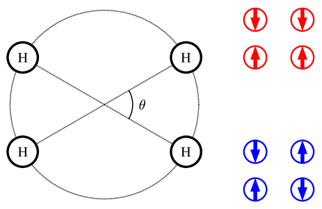
Figure 1: The H₄ system considered in paper I and introduced in Ref. Qiu et al., 2017 consists of four H atoms placed along a ring of radius $r=3.3$ bohr, controlled by an angle $\theta$. To the right we show, with different colors, the spin arrangement in the two different UHF solutions considered.

We show in the left panel of Fig. 2 the energy of the two different UHF solutions, as well as the energy of the two spin-projected UHF (SUHF) solutions that have a similar character. We also show the energy obtained in NOCI-UHF where we use the two UHF solutions plus their spin-flipped counterparts and consider the resulting two eigenvectors with “singlet” character. We also show NOCI-SUHF curves obtained using the two different SUHF solutions, as well as the two FCI lowest-lying singlet states.

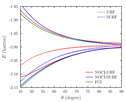
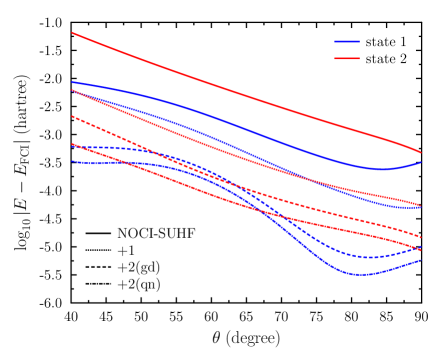
Figure 2: (Left) Energy (in hartree) of the two low-lying singlet states in the H₄ system of Fig. 1, as a function of $\theta$, computed with NOCI-UHF, NOCI-SUHF, and FCI using the 6-31G basis set. In addition, the energy of the two UHF solutions used in NOCI-UHF and the two SUHF solutions used in NOCI-SUHF is also displayed. Note that the two UHF solutions (and the two SUHF solutions) become nearly identical in energy for $\theta<70$ deg. (Right) Error in the energy, with respect to FCI, for the two low-lying singlet states. Results are shown with NOCI-SUHF and after 1 and 2 gradient descent (gd) or quasi-Newton (qn) steps.

The right panel of Fig. 2 shows the improvement to both low-lying singlet states, as a function of $\theta$, after one or two gradient descent (gd) or quasi-Newton (qn) steps have been taken, starting from the NOCI-SUHF reference subspace. The energy of both states is improved substantially even after just one iteration. Using a qn algorithm yields better results after two steps than using a gd algorithm, but in both cases the energy of both low-lying singlet states is within a mHartree of the exact FCI results.

We show in Fig. 3 the convergence profile of the gd and qn algorithms using the NOCI-UHF and NOCI-SUHF reference subspaces at $\theta=90$ deg. It is again evident that the qn algorithm reaches convergence significantly faster than the gd algorithm, as expected. The NOCI-SUHF reference subspace is significantly better than the NOCI-UHF one and convergence (with $\mu$Hartree accuracy) is reached after a handful of iterations. Using a qn algorithm, both in the case of NOCI-UHF and NOCI-SUHF, convergence of the energy for both low-lying states can be reached with a similar number of iterations.

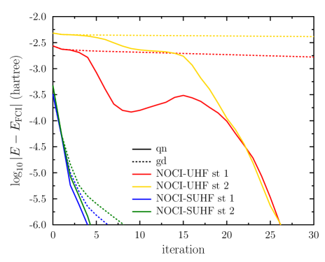
Figure 3: Convergence of the energy of the two low-lying singlet states as a function of iteration, at $\theta=90$ deg using NOCI-UHF and NOCI-SUHF and gradient descent (gd) and quasi-Newton (qn) algorithms.

III.2 LiF Avoided Crossing

We now consider the avoided crossing in the LiF potential energy curve. A correct description of the avoided crossing requires a multi-reference description Bauschlicher and Langhoff (1988). In this case, we work with a NOCI description, following our previous work Nite and Jiménez-Hoyos (2019). Explicitly, we describe the two ${}^{1}\Sigma$ states by using the restricted Hartree–Fock (RHF) determinant and the symmetric linear combination of the UHF determinant and its spin-flipped counterpart (technically, the later is not a spin singlet state, but the most significant triplet contaminant has been removed). The resulting NOCI states provide a qualitatively correct description of the avoided crossing, but the quantitative aspects are not quite correct. We have evaluated the LiF potential energy curve using the same basis set as that in Ref. Bauschlicher and Langhoff, 1988, where frozen-core FCI results were published.

We have calculated the correction in the state-averaged energy after 1 step starting from the NOCI reference subspace: sa-NOCI+1. Here, we emphasize that this computation was done by evaluation of the $F_{2}$ and $F_{3}$ matrices, without an explicit vector representation of the two states: in this case, the dimension of the FCI vector, in a basis of $m_{s}=0$ Slater determinants is $1.42\times 10^{11}$, which would render storage of the FCI vector impossible in most common computational facilities.

We show in the left panel of Fig. 4 the potential energy curves of the ground and excited state obtained with NOCI as well as sa-NOCI+1. Additionally, we show in the right panel the dipole moment for the ${}^{1}\Sigma$ states. As shown in the left panel, only a fraction of the missing correlation energy is captured by a single gd step, but significantly better results could be obtained if more steps were taken (not done in this work). As shown in the right panel, the FCI ground state dipole moment peaks near $10.5$ bohr or so, at which point the avoided crossing occurs. NOCI predicts an avoided crossing near $6.7$ bohr or so (the crossing of the two black curves), a reflection of the poor quantitative agreement with FCI. After one gd step, the avoided crossing in sa-NOCI+1 shifts by about $0.5$ bohr or so in the right direction. While this is only a modest improvement (consistent with only a fraction of the missing correlation energy recovered), we still find it encouraging.

It is interesting to compare sa-NOCI+1 with NOCI+1, where a single gd step is used to improve just the NOCI ground state. In NOCI+1, the dipole moment of the ground state is nearly identical to that of NOCI itself. This suggests that the eigenvector obtained after the diagonalization of the Hamiltonian matrix in sa-NOCI+1 has significant mixing between the ground and the excited state. It also implies that the internal contraction used in NOCI+1 (i.e., the eigenvector from NOCI) leads to larger qualitative errors in the ground state dipole moment versus sa-NOCI+1.

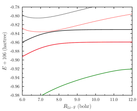
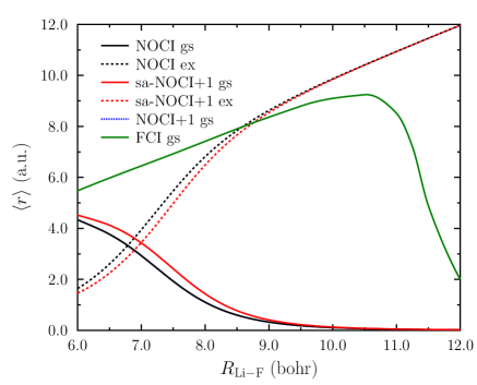
Figure 4: (Left) Ground and excited state energies in LiF with NOCI and sa-NOCI+1 (after a single gd step in a state-averaged formulation). We also show the g.s. energy obtained with NOCI+1, where only the ground state is targeted (the resulting curve is nearly indistinguishable from the sa-NOCI+1 g.s. curve). (Right) Dipole moment evaluated with the same methods. The NOCI+1 g.s. curve is in this case nearly indistinguishable from the NOCI g.s. curve. Note that after one gd step in sa-NOCI the crossing of the dipole moment is shifted by 0.5 bohr or so. The FCI g.s. results shown, obtained using a frozen-core approximation, are from Ref. Bauschlicher and Langhoff, 1988.

III.3 Formaldehyde low-energy spectrum

As a last example we consider the low-energy spectrum of the formaldehyde molecule. In a recent paper Nite and Jiménez-Hoyos (2019), we showed how a state-averaged resonating Hartree–Fock approach (sa-ResHF) can yield a good description of the low-energy spectrum of formaldehyde. Upon revisiting those results, we realized that most of the states are well described by a single SUHF determinant, with the only exception being the $1\,\,{}^{1}A_{1}$ and $3\,\,{}^{1}A_{1}$ states. In those two states (the ground and $\pi\to\pi^{\ast}$ states), the mixing between the ground RHF-like determinant and the excited $\pi\to\pi^{\ast}$ SUHF determinant is quite significant, such that the state-averaged resonating Hartree–Fock description, where the orbital optimization is done targeting the state-averaged energy, is required. The calculations in this work therefore use a single SUHF determinant for each state, except for the $1\,\,{}^{1}A_{1}$ and $3\,\,{}^{1}A_{1}$ states. Our calculations use the same aug-cc-pVDZ basis set used previously. For the triplet states we have used $m_{s}=0$ UHF determinants in SUHF solutions, although we emphasize that the spin projection was done to a triplet state.

We show in Tab. 1 the vertical excitation energies obtained by sa-ResHF and sa-(sa-ResHF)+1, where in the latter case we have carried out a single gd step in the state-averaged formalism described in this work. In this case we have also directly evaluated the $F_{2}$ and $F_{3}$ matrices without an explicit vector representation of the reference states: the dimension of the Hilbert space for $m_{s}=0$ determinants is $2.0\times 10^{19}$. We note that the calculations for each symmetry sector were carried out independently.

As shown in Tab. 1, the ground state energy is lowered by $>5$ eV after a single gd step. Nonetheless, we only see small differences (the largest differences are about $0.6$ eV) between the reference spectrum and that obtained after the gd step. Both of the ${}^{1}B_{1}$ states are shifted by around $0.55$ eV; part of that shift is likely because the calculations on each symmetry sector were done independently. If we focus on the relative energy shift within each symmetry sector, all the shifts are below $0.2$ eV, with the single outlier being the $2\,\,{}^{1}A_{1}$ state.

It is instructive, for the case of the ${}^{1}A_{1}$ states, to look at the $S_{1\ast}$ and $H_{1\ast}$ matrices. (Recall that the solution to the generalized eigenvalue problem using $H_{1\ast}$ and $S_{1\ast}$ yields the low-energy spectrum after one gd step.) They are given by (with the $H_{1\ast}$ matrix expressed in a.u.)

$$S_{1\ast} =\,\begin{pmatrix}1.0269&-0.0000&-0.0020\\ -0.0000&1.0240&0.0001\\ -0.0020&0.0001&1.0275\end{pmatrix},$$

$$H_{1\ast} =\,\begin{pmatrix}-149.4399&0.0046&0.3123\\ 0.0046&-148.6996&-0.0116\\ 0.3123&-0.0116&-149.1454\end{pmatrix}.$$

The reader may convince himself that the resulting eigenvectors have considerable mixing between the ground and the $\pi\to\pi^{\ast}$ states. Note that this is beyond the mixing present in sa-ResHF itself, as the $S_{1\ast}$ and $H_{1\ast}$ matrices are expressed in the basis of the orthonomal reference states from sa-ResHF. This significant mixing implies that the character of those two states is being adjusted in the presence of the correlation captured by the single gd step.

Table 1: Vertical excitation energies (in eV) of several low-lying singlet and triplet states of formaldehyde evaluated using the aug-cc-pVDZ basis set.

state	character	sa-ResHF	sa-(sa-ResHF)+1
singlet states
$1\,\,{}^{1}A_{1}$		0.00	0.00
$2\,\,{}^{1}A_{1}$	n $\to$ 3pb2	7.74	8.35
$3\,\,{}^{1}A_{1}$	$\pi$ $\to$ $\pi^{\ast}$	10.47	10.32
$1\,\,{}^{1}A_{2}$	n $\to$ $\pi^{\ast}$	3.61	4.04
$2\,\,{}^{1}A_{2}$	n $\to$ 3pb1	8.33	8.95
$1\,\,{}^{1}B_{1}$	$\sigma$ $\to$ $\pi^{\ast}$	9.27	9.59
$1\,\,{}^{1}B_{2}$	n $\to$ 3sa1	6.81	7.37
$2\,\,{}^{1}B_{2}$	n $\to$ 3pa1	7.84	8.39
triplet states
$1\,\,{}^{3}A_{1}$	$\pi$ $\to$ $\pi^{\ast}$	5.94	6.16
$2\,\,{}^{3}A_{1}$	n $\to$ 3pb2	8.46	8.56
$1\,\,{}^{3}A_{2}$	n $\to$ $\pi^{\ast}$	4.01	3.98
$2\,\,{}^{3}A_{2}$	n $\to$ 3pb1	9.23	9.32
$1\,\,{}^{3}B_{1}$	$\sigma$ $\to$ $\pi^{\ast}$	8.98	8.96
$1\,\,{}^{3}B_{2}$	n $\to$ 3sa1	7.52	7.57
$2\,\,{}^{3}B_{2}$	n $\to$ 3pa1	8.52	8.54

IV Conclusions

We have generalized the gradient descent and quasi-Newton algorithms presented in paper I to the optimization of a low-energy spectrum instead of just the ground state. The method presented optimizes the state-averaged energy thereby recovering the exact low-energy spectrum as the algorithm reaches convergence. The state-averaged energies along the optimization path are fully expressed in terms of transition matrix elements among the states in the reference subspace. This allows us to avoid an explicit vector representation of the intermediate wavefunctions which is crucial for systems where the dimension of the Hilbert space becomes intractable. Moreover, the algorithm defines a systematic approximation to the exact low-energy spectrum.

We have shown an application of the algorithm using a reference subspace written as a non-orthogonal configuration interaction in the case of LiF and formaldehyde. While we only carried out a single step of the algorithm in those cases, the results can be improved by carrying out a few more steps or using an improved reference subspace.

Our calculations in LiF and formaldehyde showed that in some cases there is significant mixing between the states in the reference subspace in the presence of the missing correlation captured by the algorithm. That is, even when the reference subspace was deemed as qualitatively correct, the weights of the reference configurations adjust as they evolve towards the FCI states. As a consequence of this, if the method is used to target the ground state exclusively this can lead to larger qualitative errors compared to the state-averaged description.

As presented, the method can use other type of reference subspaces such as complete active space (CAS) or more general mutli-configurational self-consistent field (MC-SCF) solutions. We plan to explore the utility of the systematic approximation here presented using those wavefunctions in the near future.

Appendix A BFGS Update

We discuss in this appendix the form of the search direction $p_{1}=-B_{1}g_{1}$, with $B_{1}$ constructed from a Broyden-Fletcher-Goldfarb-Shanno (BFGS) Broyden (1970); Fletcher (1970); Goldfarb (1970); Shanno (1970) update formula (starting from $B_{0}=I$). Let

$$s_{0} =\,Z_{1}-Z_{0}=Z_{1},$$ (29)

$$y_{0} =\,g_{1}-g_{0},$$ (30)

which yields $s_{0}=-\sigma_{\ast}g_{0}$ and

$$(y_{0})^{k}_{x}=H_{x}^{l}(\alpha_{1}-\alpha_{0})_{l}^{k}+H_{x}^{y}H_{y}^{l}(\beta_{1})_{l}^{k}.$$ (31)

Defining $\rho_{0}\equiv 1/[(s_{0})^{x}_{k}(y_{0})^{k}_{x}]$, the BFGS update takes the form

$${}_{s}^{k}(B_{1})_{l}^{t} =\,{}_{s}^{k}(B_{0})_{l}^{t}$$

$$-\,\rho_{0}\,\,{}_{s}^{k}(B_{0})_{m}^{x}(y_{0})^{m}_{x}(s_{0})^{t}_{l}-\rho_{0}(s_{0})^{k}_{s}(y_{0})^{x}_{m}\,\,{}_{x}^{m}(B_{0})_{l}^{t}$$

$$+\,\rho_{0}^{2}\Big{[}\rho^{-1}_{0}+(y_{0})^{x}_{m}\,\,{}_{x}^{m}(B_{0})_{n}^{y}(y_{0})^{n}_{y}\Big{]}(s_{0})_{s}^{k}(s_{0})^{t}_{l}$$ (32)

We now carry an explicit evaluation of $p_{1}=-B_{1}g_{1}$. We note that

$$\rho^{-1}_{0} =\,-\sigma_{\ast}\mathrm{Tr}\left\{\alpha_{0}F_{2}(\alpha_{1}-\alpha_{0})+\alpha_{0}F_{3}\beta_{1}\right\},$$

$$[y_{0}y_{0}] \equiv\,(y_{0})_{k}^{x}(y_{0})^{k}_{x}$$

$$=\,\mathrm{Tr}\left\{(\alpha_{1}-\alpha_{0})F_{2}(\alpha_{1}-\alpha_{0})+(\alpha_{1}-\alpha_{0})F_{3}\beta_{1}\right.$$

$$+\,\left.\beta_{1}F_{3}(\alpha_{1}-\alpha_{0})+\beta_{1}F_{4}\beta_{1}\right\},$$

$$[s_{0}g_{1}] \equiv\,(s_{0})_{k}^{x}(g_{1})^{k}_{x}$$

$$=\,-\sigma_{\ast}\mathrm{Tr}\left\{\alpha_{0}F_{2}\alpha_{1}+\alpha_{0}F_{3}\beta_{1}\right\},$$

$$[y_{0}g_{1}] \equiv\,(y_{0})_{k}^{x}(g_{1})^{k}_{x}$$

$$=\,\mathrm{Tr}\left\{(\alpha_{1}-\alpha_{0})F_{2}\alpha_{1}+(\alpha_{1}-\alpha_{0})F_{3}\beta_{1}\right.$$

$$+\,\left.\beta_{1}F_{3}\alpha_{1}+\beta_{1}F_{4}\beta_{1}\right\}.$$

Therefore, $p_{1}$ takes the form

$$(p_{1})^{k}_{x}=H_{x}^{l}(\alpha^{\prime}_{1})^{k}_{l}+H_{x}^{y}H_{y}^{l}(\beta^{\prime}_{1})^{k}_{l},$$ (33)

with

$$\alpha^{\prime}_{1} =\,\alpha_{1}-\sigma_{\ast}\rho_{0}^{2}(\rho_{0}^{-1}+[y_{0}y_{0}])[s_{0}g_{1}]\alpha_{0}$$

$$-\,\rho_{0}[s_{0}g_{1}](\alpha_{1}-\alpha_{0})+\sigma_{\ast}\rho_{0}[y_{0}g_{1}]\alpha_{0},$$ (34)

$$\beta^{\prime}_{1} =\,\beta_{1}-\rho_{0}[s_{0}g_{1}]\beta_{1}.$$ (35)

References

- Szabo and Ostlund (1989) A. Szabo and N. S. Ostlund, Modern Quantum Chemistry: Introduction to Advanced Electronic Structure Theory (McGraw-Hill, New York, 1989).
- Jiménez-Hoyos (2020) C. A. Jiménez-Hoyos, Approaching the full configuration interaction ground state from an arbitrary wavefunction with gradient descent and quasi-Newton algorithms (2020), eprint arXiv:2010.02027.
- Sundstrom and Head-Gordon (2014) E. J. Sundstrom and M. Head-Gordon, J. Chem. Phys. 140, 114103 (2014).
- Jensen et al. (2018) K. T. Jensen, R. L. Benson, S. Cardamone, and A. J. W. Thom, J. Chem. Theory Comput. 14, 4629 (2018).
- Jiménez-Hoyos et al. (2012) C. A. Jiménez-Hoyos, T. M. Henderson, T. Tsuchimochi, and G. E. Scuseria, J. Chem. Phys. 136, 164109 (2012).
- Nite and Jiménez-Hoyos (2019) J. Nite and C. A. Jiménez-Hoyos, J. Chem. Theory Comput. 15, 5343 (2019).
- Nocedal and Wright (2006) J. Nocedal and S. J. Wright, Numerical Optimization (Springer, New York, 2006), 2nd ed.
- Broyden (1970) C. G. Broyden, IMA J. Appl. Math. 6, 76 (1970).
- Fletcher (1970) R. Fletcher, Comput. J. 13, 317 (1970).
- Goldfarb (1970) D. Goldfarb, Math. Comp. 24, 23 (1970).
- Shanno (1970) D. F. Shanno, Math. Comp. 24, 647 (1970).
- Qiu et al. (2017) Y. Qiu, T. M. Henderson, and G. E. Scuseria, J. Chem. Phys. 146, 184105 (2017).
- Bauschlicher and Langhoff (1988) C. W. Bauschlicher and S. R. Langhoff, J. Chem. Phys. 89, 4246 (1988).
- Nite and Jiménez-Hoyos (2019) J. Nite and C. A. Jiménez-Hoyos, Efficient multi-configurational wavefunction method with dynamical correlation using non-orthogonal configuration interaction singles and doubles (NOCISD) (2019), eprint ChemRxiv:11369641.