2-Step Sparse-View CT Reconstruction with a Domain-Specific Perceptual Network

Abstract

Computed tomography is widely used to examine internal structures in a non-destructive manner. To obtain high-quality reconstructions, one typically has to acquire a densely sampled trajectory to avoid angular undersampling. However, many scenarios require a sparse-view measurement leading to streak-artifacts if unaccounted for. Current methods do not make full use of the domain-specific information, and hence fail to provide reliable reconstructions for highly undersampled data.

We present a novel framework for sparse-view tomography by decoupling the reconstruction into two steps: First, we overcome its ill-posedness using a super-resolution network, SIN, trained on the sparse projections. The intermediate result allows for a closed-form tomographic reconstruction with preserved details and highly reduced streak-artifacts. Second, a refinement network, PRN, trained on the reconstructions reduces any remaining artifacts.

We further propose a light-weight variant of the perceptual-loss that enhances domain-specific information, boosting restoration accuracy. Our experiments demonstrate an improvement over current solutions by $4$ dB.

1 Introduction

Since invented in 1972, Computed Tomography (CT) has quickly been recognized as an essential non-destructive modality for industrial inspection [7], medical diagnosis [30] or material sciences [43]. CT is a textbook example of computational imaging, where a physical quantity is encoded in the measured data by an image formation model and then reconstructed by inverting this forward model. In the case of X-ray CT, an image of the attenuation coefficient is reconstructed from projections acquired in a circular acquisition. Under orthographic projection, this model becomes the Radon transform. Discretized measurements of the Radon transform are called sinograms and their inversion is well-studied. The most prominent approach is a direct inversion with a closed-form solution called Filtered Back-Projection (FBP) [30].

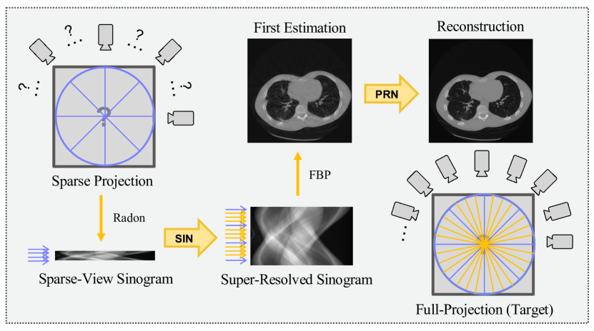
Figure 1: Proposed two-step strategy for the sparse-view CT problem, where projections are not enough to recover a high-quality reconstruction. To obtain a reliable reconstruction from sparse projections, a SIN first super-resolves the projection image in one dimension. This allows a direct reconstruction via FBP. Then the PRN removes remaining artifacts.

Accurate reconstruction with FBP requires sufficient angular sampling in terms of the Crowther-criterion [6] derived from the Shannon-Nyquist sampling theorem. If violated, aliasing artifacts appear as streak-artifacts that drastically reduce diagnostic quality. This setting is called Sparse-View CT (SV-CT) and arises in many practical applications, addressing motion compensation [9] or dose-reduction [10, 48].

A number of approaches have been proposed to overcome the ill-posedness of SV-CT by incorporating prior knowledge into the reconstruction algorithm. Traditionally, Iterative Reconstruction (IR) is used to optimize a data-fidelity term coupled with appropriate priors [24, 54, 41]. For example, the popular total variation (TV) prior assumes piece-wise constant objects for CT [38]. Recently, learning-based reconstruction algorithms have attracted a lot of attention [1]. Prominent examples are convolutional neural network (CNN)-based models designed to remove artifacts in reconstruction domain [22] or unrolled networks mimicking the data-fidelity driven IR [33].

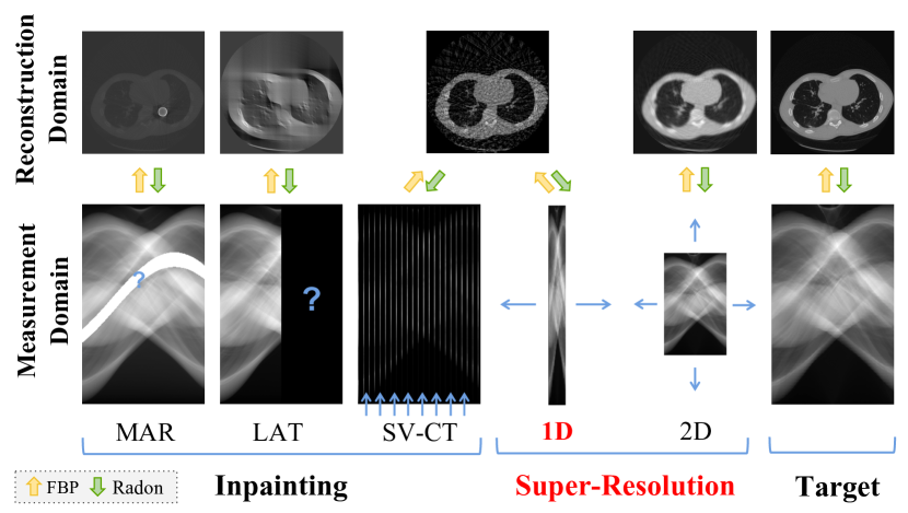
Figure 2: Different problems arising in tomographic imaging and their relations to our 1D-super-resolution task, such as metal artifact removal (MAR) and limited angle tomography (LAT). SV-CT is at the intersection of inpainting and super-resolution when viewed in measurement domain.

A less common approach is to interpret SV-CT as a super-resolution or inpainting problem, where the missing information is interpolated between the sparse projections. A sparse-view sinogram can be either inpainted or 1D-super-resolved. Either way, 1D-upsampling of a sinogram is more constrained than its 2D-counterpart [19] of natural images, since the sinogram data vary smoothly along the angular dimension [15]. Other typical tomographic problems with similar formulations include metal artifact removal and limited angle tomography, see Fig. 2.

Sinogram inpainting did not attract much attention compared to iterative approaches. This is because capturing the intricate representations of sinograms turns out to be an extremely challenging task [27, 40, 23]. However, the fast development of deep learning now enables us to efficiently capture low-dimensional representations of data in various image domains. These technological advances motivate us to consider the possibilities of tackling SV-CT with learning-based super-resolution.

In particular, we argue and will demonstrate that image-processing in the measurement domain is favored over post-reconstruction processing. This is because sinogram-based methods prevent the generation of streak artifacts that are difficult to remove using local processing (e.g., CNNs) because they are widely distributed over the image domain.

In this work, we propose a two-step architecture that learns super-resolution in the sinogram domain and then removes the remaining artifacts in the image domain. The core idea is outlined in Fig. 1. The following summarizes our main contributions:

• A novel 2-step reconstruction approach in both measurement and image domain. It ensures maximum detail-preservation compared to single-step networks.

• A novel domain-specific, light-weight perceptual loss that outperforms the VGG-based perceptual loss [18] in terms of accuracy, memory and time efficiency.

• Loss functions and submodules tailored to sinogram-domain tasks, and an extensive ablation study that analyzes the effectiveness of each proposed module.

• Demonstration of accurate reconstructions for high compression ratios while achieving a significant performance gain (over $4$ dB PSNR) compared to state-of-the-art algorithms.

2 Related Work

Learned Image Reconstruction

Recent advances in the reconstruction community seek to learn better image priors from available data [33]. Two prominent strategies stand out: Postprocessing networks (PN) and Operator-based learning (OBL).

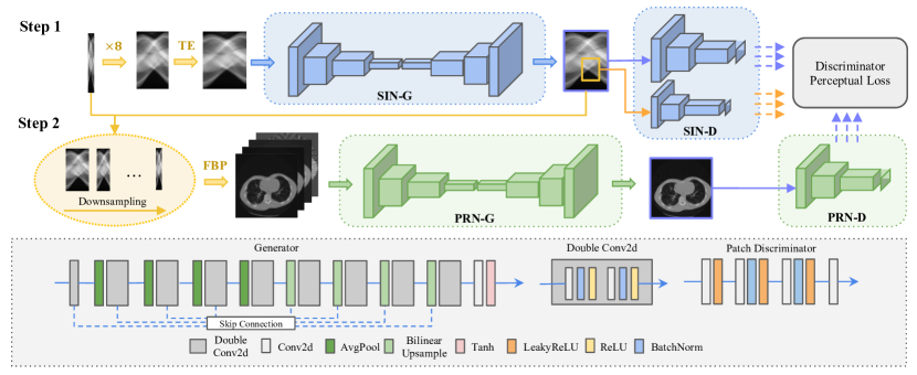
Figure 3: Network Architecture of our proposed SIN-4c-PRN model. Top: In step one, we linearly upsample a sparse-view sinogram and preprocess with our Two-Ends (TE) flipping method as input to the SIN model. In step two, the super-resolved sinogram is 1D-downsampled by different factors. FBP reconstructions from the set of sinograms are concatenated as a cascaded input to the PRN. The patch discriminators SIN-D and PRN-D calculate pixel-wise adversarial losses of global or local generated images. Additionally, each discriminator calculates a discriminator perceptual loss that enhances the generator’s perceptual knowledge. Bottom: Detailed architecture of our SIN and PRN models.

A single-step PN removes aliasing artifacts after a direct inversion with closed-form solutions such as FBP. Variants of different neural networks are proposed to learn PN models to eliminate streak artifacts, such as GoogLeNet [45], DenseNet [50] or TomoGAN [29]. An improved version was presented by Han and Ye [14], showing that networks fulfilling the frame-condition yield improved outcomes. A downside of these PN-based methods is their inability to constrain their output by relating it to the measured data.

With OBL a differentiable forward model is included into the network. Most OBL frameworks unroll IR, such as gradient descent, and learn the gradient of an image prior that is applied during each iteration. For SV-CT, Chen et al. [4] demonstrated state-of-the-art performance with OBL. A more general approach to learning a data-driven inversion of linear inverse problems are Neumann networks introduced by Gilton et al. [12].

An entirely different approach from iterative reconstruction with learned priors is to reuse an arbitrary denoising method for images as a proximal operator. This approach was pioneered by Venkatakrishnan et al. [42], referred to Plug-and-Play (P&P)-priors and can be combined with learned denoising.

Image Super-Resolution $\&$ Inpainting

A different approach to solve SV-CT poses it as a super-resolution or inpainting problem in the measurement domain. This is advantageous because sinograms do not yet suffer from aliasing artifacts. U-Nets [37] and generative adversarial networks (GAN) [13] have demonstrated strong performance in this task by either considering the whole sinogram [8, 11, 39, 46] or local patches [25].

Recent approaches in other tomographic applications (Fig. 2) combine learning in both sinogram and image domain to leverage the advantages of both representations. For example, Zhao et al. [52] proposed an unsupervised sinogram inpainting network trained in both domains in a cycle for limited angle tomography. One of the first to propose adding a Radon inversion layer to directly couple measurement and reconstruction domain was Wúrfl et al.[44]. The idea of dual-domain training was borrowed by DuDoNet [28] to first inpaint missing information due to metal-artifacts, see Fig. 2 and refine the subsequent reconstruction.

Perceptual Losses

GAN loss functions are often paired with a perceptual loss to produce visually convincing images. Perceptual loss was introduced in the seminal work by Johnson et al. [18] to tackle the long-standing problem that pixel-based loss-functions, such as the one using the $l_{2}$-norm, struggling to capture higher-level feature information. Perceptual losses are increasingly incorporated in many imaging algorithms showing superior performance while maintaining a reasonable convergence speed [49]. Yet, there is an ongoing debate about whether the natural color image features apply to images with a drastically different formation model and diverse content. In the medical imaging setting, domain-specific perceptual networks were proposed to account for the domain change [26, 34]. These methods require pre-training of an additional network which increases the complexity of the complete training pipeline, making it harder to reproduce results.

3 Proposed Approach

We propose a two-step framework with novel loss-functions tailored for SV-CT, shown in Fig. 3. First, we augment a sparse-view sinogram by 1D linear-interpolation and Two-Ends preprocessing, which accounts for boundary artifacts. The Sinogram Inpainting Network (SIN) generates a reliable super-resolved sinogram so that the object can be reconstructed without strong streak artifacts via FBP. While SIN successfully restores a full-view sinogram, small imperfections still lead to some less-severe, more localized artifacts. In the final refinement step, our Postprocessing Refining Network (PRN) removes such artifacts to obtain a high-quality reconstruction.

This section discusses the network architectures, introduces our novel discriminator-perceptual loss, and outlines the optimization procedure.

3.1 Two-Ends Sinogram Flipping

Boundary pixels have only one-sided neighborhood information. This quickly results in border blurriness detrimental for reconstruction. We present a simple two-ends method that appends angles at the two ends of sparse-view sinograms as outlined in Fig. 4.

Note that we only leverage data already present in the measurements. This is because under orthographic projection, the total intensity detected from angle $\theta$ is a flipped version of the projection at angle $\theta+\pi$. This allows us to repeat the first and last few angles of a sinogram by flipping them along the detector axis and appending them to the other end.

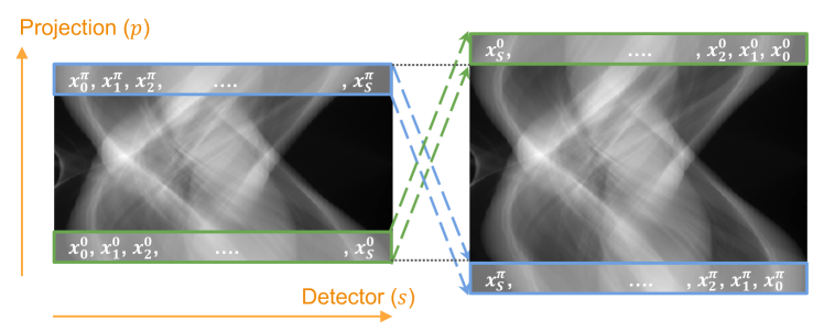
Figure 4: We avoid boundary artifacts during convolutions by reusing projections on both ends of the sinogram.

3.2 Network Architectures

Following previous works in learned CT-reconstruction, we use the GAN [13] framework in both steps. We first describe our adapted U-Net generators and global and local patch discriminators [16, 17] in detail. Then we introduce our SIN-4c-PRN architecture based on SIN and PRN.

Adapted U-Net Generators

A U-Net is a CNN that includes an encoding-decoding process with skip connections [37]. We made the following adaptions to the U-Net modules in our framework: Four average-pooling and bilinear-upsampling layers, each followed by several deep convolutional layers. We keep skip-connections at each resolution level to ensure low-level feature consistency.

We find that resizing operations such as pooling and bilinear layers restore smooth sinusoids essential for tomographic reconstruction. In contrast, half-strided convolutions introduce severe checkerboard artifacts [32] as in our experiments.

We further replace max-pooling with average-pooling, since a differentiable operator is preferable over subdifferentials for restoration tasks [53, 47]. The preservation of gradients maximally recovers measurement-domain information. Otherwise, if the high-frequencies produced by max-pooling are misaligned, errors will be amplified by the following FBP operation.

Patch Discriminators

Inspired by Isola et al. [17], our discriminators include four convolution layers that downscale the input by a factor of four and output image patches. Pixel-wise probabilities of these patches being real or fake are then calculated as adversarial losses described in Sec. 3.4. We also keep the discriminators in relatively low dimensional feature space ($\leq 256$ kernels) for ease of training without compromising performance [2].

Sinogram Inpainting Network (SIN)

The proposed SIN fills in the missing projections by directly learning from sparse-view to full-view sinograms. The adapted U-Net generates super-resolved sinograms from an initial linear estimation, trained simultaneously with two patch discriminators that focus on either global or local descriptions of the generated sinograms. Specifically, the local discriminator randomly picks $1/4\times 1/4$ local patches from super-resolved sinograms to enhance local sinusoidal details.

Postprocessing Refinement Network (PRN)

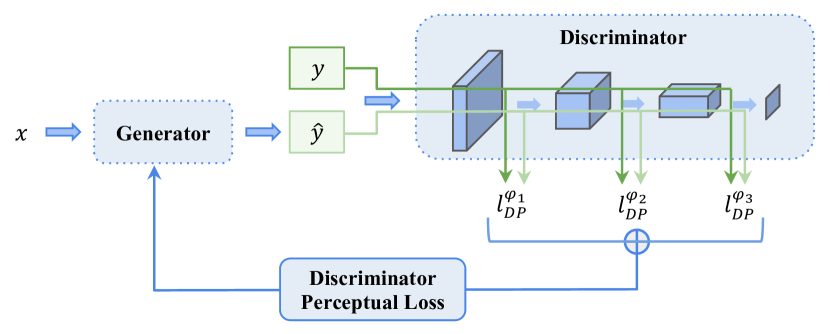
Figure 5: Discriminator Perceptual Loss. The image pair $\hat{y}$ generated from the input $x$, and the target image $y$ are compared at each activation layer output $\phi_{j}$ in the discriminator. Pixel-wise losses are calculated for updating the generator.

PRN is connected to SIN by the FBP operator, and it includes a U-Net and a patch discriminator.

One major consideration in designing a second-step network is to prevent propagation of errors introduced by our SIN. To solve this, we introduce a set of reconstructions from multi-resolution sinograms for our PRN to learn from. We observe that SV-CT reconstructions already show sharp partial information although severely obscured by aliasing artifacts. Effective use of such information can be achieved by constructing a pool of diverse features for the network to learn from.

In particular, we downsample the SIN-inpainted sinograms along the angular axis by factors of 2 and 4. Then four different FBP reconstructions from sparse, $2\times$downsampled, $4\times$downsampled, and fully-inpainted sinograms are concatenated as a 4-channel input to the PRN.

3.3 Discriminator Perceptual Network

Perceptual losses have proven to significantly enhance the ability of networks to generate images with high perceptual quality [49] when compared to traditional pixel-wise losses. The original perceptual loss computes the $l_{2}$ norm of generated and target image pairs through a pre-trained Visual Geometry Group (VGG) network [18], which serves as a feature extractor that enforces high-level feature fidelity.

We propose a novel Discriminator Perceptual (DP) loss that is easy to incorporate into the formulation and especially suitable for domain-specific tasks. It interprets the first few layers of a discriminator as a feature extractor, which is trained simultaneously with the generator on the current problem, and encourages feature-level similarity, see Fig. 5. The DP-loss is computed in a similar fashion as the original perceptual-loss with VGG.

We find out that introducing the DP-loss promotes stability in our GAN training procedure. For example, we can train the discriminator until convergence at each iteration of the minimax game. An incremental strategy for training GANs with DP-loss is provided in the supplementary material for further reference.

DP loss is calculated by the $l_{2}$ norms of the error between outputs of each activation layer $\phi_{j}$ in the discriminator with respect to the input pair consisting of the generated image $\hat{y}$ and the target image $y$. While one can choose any such layer $j$ in a discriminator, we compute the averaged norm for each $\phi_{j}$ before the last one (i.e., we do not include the discriminator output layer):

$$\mathcal{L}_{DP}(\hat{y},y)=\frac{1}{N}\sum_{j=1}^{N}\frac{1}{C_{j}H_{j}W_{j}}\|\phi_{j}(\hat{y})-\phi_{j}(y)\|_{2}^{2}$$ (1)

where $C_{j}$ is the number of channels, $H_{j}$, $W_{j}$ are height and width of the output at $\phi_{j}$, respectively, and $N$ is the number of activation layers we use.

3.4 Optimization

Adversarial loss

In the GAN-framework [13], the generator is augmented by a discriminator that discerns real and synthesized images. During training, the generator and the discriminator compete in a min-max game that leads to the adversarial loss.

Given a corrupted image $x$ and a target image $y$, we formulate the optimization target as follows:

$$\min_{G}\max_{D}V(G,D)= \mathbb{E}_{y\sim target}[\log D(y)]+$$ (2)

$$\mathbb{E}_{x\sim corrupt}[\log(1-D(G(x))],$$

where $G$ and $D$ represent the generator and discriminator networks, respectively.

Specifically, in SIN, the input $x\in\mathbb{R}^{S\times P}$ is the preprocessed sparse-view sinogram to $S$ detector pixels and $P$ angles and target $y\in\mathbb{R}^{S\times P^{\prime}}$ is a preprocessed full-view sinogram. Local discriminators compare $G(x)_{patch}$ and $y_{patch}\in\mathbb{R}^{\lfloor S/4\rfloor\times\lfloor P^{\prime}/4\rfloor}$, which are small patches from the sinogram randomly chosen from $G(x)$ and $y$, respectively. In PRN, $x$ and $y\in\mathbb{R}^{S\times S}$ form the input and target reconstructions pair.

Content Loss

Besides the adversarial loss, we ensure the data fidelity of the generated images by applying an $l_{1}$-norm based pixel-reconstruction loss:

$$\begin{split}\mathcal{L}_{c}(\hat{y},y)=\|\hat{y}-y\|_{1},\end{split}$$ (3)

where $\hat{y}$ is the generated and $y$ the target image. The content loss is calculated in both SIN and PRN. As suggested in [51], we choose the $l_{1}$ loss since our experiments showed slightly sharper reconstructions compared to the $l_{2}$ loss.

High-Frequency (HF) Loss

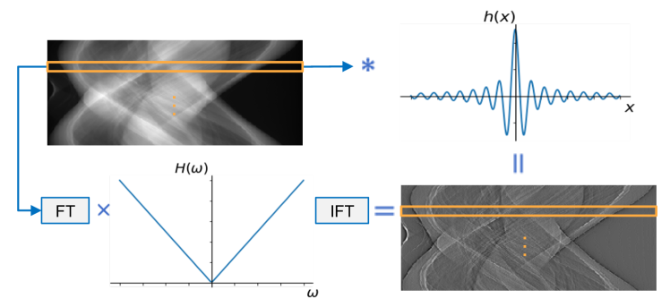
Figure 6: Applying Ramp filter to a sinogram preserves high frequency features. The filter is applied along one dimension in the frequency or spatial domains. Since the Ramp operator is back-propagatable [36], losses can be defined on the ramp-filtered signal.

Neural networks tend to prioritize learning of low-frequency features during training [35]. While it might be acceptable for PRN since tomographic reconstructions tend to be relatively smooth, it is of critical importance for SIN where high-frequency information is essential for correct reconstructions. This is because FBP requires ramp filtering [30] which is a high-pass filter compensating for oversampling the low-frequencies, as illustrated in Fig. 6.

To incorporate this CT-domain knowledge, we enforce our SIN to restore an accurate ramp-filtered sinogram by defining a high-frequency loss:

$$\mathcal{L}_{HF}(\hat{y},y)=\|\hat{y}\ast h-y\ast h\|_{1},$$ (4)

where $h$ is the ramp kernel in the spatial domain, and $\ast$ denotes convolution. Note that the high-frequency loss is fully backpropagatable [36].

Total Objective

Finally, the total objective function of the SIN generator is the weighted sum of the four losses mentioned above:

$$G_{SIN}\text{*}=arg\min_{G}[\lambda_{1}\mathcal{L}_{adv}(G)+\lambda_{2}\mathcal{L}_{c}+\lambda_{3}\mathcal{L}_{DP}+\lambda_{4}\mathcal{L}_{HF}],$$ (5)

where $\mathcal{L}_{adv}$ defines the adversarial loss [13] (details in the supplementary material) and $\lambda_{i}$ are empirically chosen weighting parameters. Based on our experiments, we set $\lambda_{1}=1,\lambda_{2}=50,\lambda_{3}=20,\lambda_{4}=50$. All discriminator adversarial losses are assumed a weight equal to one.

Similarly, the total objective function for the PRN is:

$$G_{PRN}\text{*} =arg\min_{G}[\lambda_{1}\mathcal{L}_{adv}(G)+\lambda_{2}\mathcal{L}_{c}+\lambda_{3}\mathcal{L}_{DP}],$$ (6)

where all parameters $\lambda_{i}$ are chosen the same as for SIN.

4 Experiments

Our experiments are performed on the open-source TCIA LDCT-and-Projection-Dataset [5, 31]. We extensively evaluate our methodology both qualitatively using samples of chest, abdomen, and head images and quantitatively using the Structural Similarity Index Measure (SSIM) and Peak Signal-to-Noise Ratio (PSNR).

We define a full-view target sinogram $y^{*}\in\mathbb{R}^{S\times P^{*}}$ to have $S=320$ detector pixels and $P^{*}=180$ uniformly-distributed angles over $\pi$. The sparse-view input includes 23 angles sampled from $y^{*}$ once every eight projections, and the reconstructed image have a resolution of $320\times 320$ pixels. Due to the proposed two-ends preprocessing, we take six angles from each end of $y^{*}$ to generate a 192-angle sinogram $y\in\mathbb{R}^{S\times(P^{*}+12)}$ as the ground-truth for SIN.

4.1 Datasets

Our dataset contains 5394 images resized to $320\times 320$ stemming from 68 patients taken from the TCIA dataset. Additionally, we augment each sample with a random affine transform to increase data diversity during training. Note that this transformation is performed on the reconstructions, which leads to significant variation in the sinogram domain. We then extract a set of around 500 images from the dataset patient-wise for testing. Once we choose a patient for testing, we remove all data related to this patient from the training set to avoid inter-slice correlation. Full-view sinograms are generated using parallel-beam (orthographic) projections over an angular range of 180 degree, which define the target set for SIN.

4.2 Training Details

Following the standard GAN procedure [13, 16], the generator and both global and local discriminators are trained alternatively. The ADAM [21] solver with momentum parameters $\beta_{1}=0.5$ and $\beta_{2}=0.999$ are used to optimize all networks. We set the learning rate to 0.0001 and run 100 epochs or until convergence for all experiments. For further details on the training procedure, please consult the supplementary material.

\begin{overpic}[width=433.62pt]{images/interm_result/BL1.png} \put(17.0,6.0){{\color[rgb]{1,.5,0}33.56}} \put(17.0,16.0){{\color[rgb]{1,.5,0}0.917}} \end{overpic}

(a) Linear

\begin{overpic}[width=433.62pt]{images/interm_result/SIN-sino.png} \put(17.0,6.0){{\color[rgb]{1,.5,0}40.22}} \put(17.0,16.0){{\color[rgb]{1,.5,0}0.978}} \end{overpic}

(b) SIN

\begin{overpic}[width=433.62pt]{images/interm_result/gt1.png} \put(17.0,6.0){{\color[rgb]{1,.5,0}PSNR}} \put(17.0,16.0){{\color[rgb]{1,.5,0}SSIM}} \end{overpic}

(c) Ground Truth

\begin{overpic}[width=433.62pt]{images/interm_result/SIN-FBP.png} \put(5.0,90.0){{\color[rgb]{1,.5,0}31.96}} \put(48.0,90.0){{\color[rgb]{1,.5,0}0.828}} \end{overpic}

(d) SIN

\begin{overpic}[width=433.62pt]{images/interm_result/4c.png} \put(5.0,90.0){{\color[rgb]{1,.5,0}33.15}} \put(48.0,90.0){{\color[rgb]{1,.5,0}0.859}} \end{overpic}

(e) SIN-4c-PRN

\begin{overpic}[width=433.62pt]{images/interm_result/gt2.png} \put(5.0,90.0){{\color[rgb]{1,.5,0}PSNR}} \put(48.0,90.0){{\color[rgb]{1,.5,0}SSIM}} \end{overpic}

(f) Ground Truth

Figure 7: Our results in both measurement and reconstruction domains with zoom-in details compared to linear interpolation.

\begin{overpic}[width=433.62pt]{images/baselines/sparse5.png} \put(5.0,90.0){{\color[rgb]{1,.5,0}21.52}} \put(50.0,90.0){{\color[rgb]{1,.5,0}0.438}} \end{overpic}

\begin{overpic}[width=433.62pt]{images/baselines/Fista5.png} \put(5.0,90.0){{\color[rgb]{1,.5,0}29.90}} \put(50.0,90.0){{\color[rgb]{1,.5,0}0.805}} \end{overpic}

\begin{overpic}[width=433.62pt]{images/baselines/cgan5.png} \put(5.0,90.0){{\color[rgb]{1,.5,0}28.87}} \put(50.0,90.0){{\color[rgb]{1,.5,0}0.731}} \end{overpic}

\begin{overpic}[width=433.62pt]{images/baselines/NN5.png} \put(5.0,90.0){{\color[rgb]{1,.5,0}27.35}} \put(50.0,90.0){{\color[rgb]{1,.5,0}0.619}} \end{overpic}

\begin{overpic}[width=433.62pt]{images/baselines/ours5.png} \put(5.0,90.0){{\color[rgb]{1,.5,0}32.76}} \put(50.0,90.0){{\color[rgb]{1,.5,0}0.861}} \end{overpic}

\begin{overpic}[width=433.62pt]{images/baselines/gt5.png} \put(5.0,90.0){{\color[rgb]{1,.5,0}PSNR}} \put(50.0,90.0){{\color[rgb]{1,.5,0}SSIM}} \end{overpic}

\begin{overpic}[width=433.62pt]{images/baselines/sparse2.png} \put(5.0,90.0){{\color[rgb]{1,.5,0}24.14}} \put(50.0,90.0){{\color[rgb]{1,.5,0}0.522}} \end{overpic}

\begin{overpic}[width=433.62pt]{images/baselines/Fista2.png} \put(5.0,90.0){{\color[rgb]{1,.5,0}30.94}} \put(50.0,90.0){{\color[rgb]{1,.5,0}0.847}} \end{overpic}

\begin{overpic}[width=433.62pt]{images/baselines/cgan2.png} \put(5.0,90.0){{\color[rgb]{1,.5,0}32.16}} \put(50.0,90.0){{\color[rgb]{1,.5,0}0.796}} \end{overpic}

\begin{overpic}[width=433.62pt]{images/baselines/NN2.png} \put(5.0,90.0){{\color[rgb]{1,.5,0}29.68}} \put(50.0,90.0){{\color[rgb]{1,.5,0}0.788}} \end{overpic}

\begin{overpic}[width=433.62pt]{images/baselines/ours2.png} \put(5.0,90.0){{\color[rgb]{1,.5,0}36.29}} \put(50.0,90.0){{\color[rgb]{1,.5,0}0.913}} \end{overpic}

\begin{overpic}[width=433.62pt]{images/baselines/gt2.png} \put(5.0,90.0){{\color[rgb]{1,.5,0}PSNR}} \put(50.0,90.0){{\color[rgb]{1,.5,0}SSIM}} \end{overpic}

\begin{overpic}[width=433.62pt]{images/baselines/sparse6.png} \put(5.0,90.0){{\color[rgb]{1,.5,0}23.05}} \put(50.0,90.0){{\color[rgb]{1,.5,0}0.490}} \end{overpic}

(a) Sparse-View

\begin{overpic}[width=433.62pt]{images/baselines/Fista6.png} \put(5.0,90.0){{\color[rgb]{1,.5,0}32.10}} \put(50.0,90.0){{\color[rgb]{1,.5,0}0.867}} \end{overpic}

(b) FISTA-TV [3]

\begin{overpic}[width=433.62pt]{images/baselines/cgan6.png} \put(5.0,90.0){{\color[rgb]{1,.5,0}30.19}} \put(50.0,90.0){{\color[rgb]{1,.5,0}0.778}} \end{overpic}

(c) cGAN [11]

\begin{overpic}[width=433.62pt]{images/baselines/NN6.png} \put(5.0,90.0){{\color[rgb]{1,.5,0}27.76}} \put(50.0,90.0){{\color[rgb]{1,.5,0}0.650}} \end{overpic}

(d) Neumann [12]

\begin{overpic}[width=433.62pt]{images/baselines/ours6.png} \put(5.0,90.0){{\color[rgb]{1,.5,0}34.31}} \put(50.0,90.0){{\color[rgb]{1,.5,0}0.915}} \end{overpic}

(e) SIN-4c-PRN

\begin{overpic}[width=433.62pt]{images/baselines/gt6.png} \put(5.0,90.0){{\color[rgb]{1,.5,0}PSNR}} \put(50.0,90.0){{\color[rgb]{1,.5,0}SSIM}} \end{overpic}

(f) Ground Truth

Figure 8: Baseline results with zoom-in details. From top to bottom row: Chest: In our SIN-4c-PRN result, both soft tissues in the black region of the body and sharp edges of bones are maximally recovered compared to other methods. Abdomen: Soft tissues with low contrast, such as in the green box are hard to recover from sinograms and pose a significant challenge for our networks. Head: The high-frequency details in the nose and bone regions are reconstructed while others either fail or over-smooth them.

4.3 Qualitative Results

We first show our results in both measurement and reconstruction domains in Fig. 7. Compared with a naive linear interpolation, our super-resolved sinograms accurately restore the smooth sinusoidal structures. It is nearly impossible to discern difference between SIN-generated and ground-truth sinograms. A subsequent reconstruction in Fig. 7(d) obtained by FBP shows an artifact-reduced reconstruction that resembles the target image. However, there remains a novel type of less severe artifacts. These localized artifacts can be efficiently removed by PRN in the second step. The final result of our SIN-4c-PRN preserves details such as bones and soft-tissue contrast.

Comparison to State-of-the-Art

In Fig. 8, we further compare our SIN-4c-PRN model to state-of-the-art CT reconstruction approaches.

FISTA-TV [3] is a powerful iterative reconstruction algorithm that employs TV-based regularization. We use the implementation in the open-source toolkit ToMoBAR [20]. To select the optimal hyperparameters of FISTA-TV, we perform a grid-search and choose the set with the best visual results. FISTA-TV preserves edges well, but the reconstructions are over-smoothed, which is a well-known weakness of the TV-prior.

We further compare with a learning-based sinogram inpainting network that uses a conditional-GAN (cGAN) based on an Encoding-Decoding U-Net [11] with strided-convolutions. We implement their architecture and tuned hyper-parameters to obtain the best results. Our experiments show that checkerboard artifacts still exist in generated sinograms due to the strided convolutions, see supplementary material for example images. And these artifacts are further amplified in reconstructions. Note that the original work uses much lower undersampling factors than we are aiming for in this paper, which might explain the discrepancy to their findings.

Finally, we compare against our own PyTorch implementation of Neumann networks [12]. Neumann networks are a variant of unrolled optimization that learns a CNN-based regularizer. They have proven to yield great results in solving super-resolution and MRI problems. Note that unrolling networks require a back-propagatable tomography operator, for which we use torch-radon [36]. Despite extensive tuning of hyper-parameters, our implementation fails to remove streak artifacts and over-smoothness.

4.4 Quantitative Results

For a quantitative evaluation we measure the PSNR and SSIM statistics within a circular region-of-interest using our test dataset. Table 1 shows that our proposed SIN-4c-PRN model significantly improves the reconstruction accuracy compared to the other state-of-the-art reconstruction methods discussed earlier. In particular, our model improves the average PSNR by over $4$ dB and SSIM by $5\%$, with narrowed variance.

Method	PSNR ($\sigma$)	SSIM ($\sigma$)
FISTA-PD-TV [3]	30.61 (2.67)	0.839 (0.036)
cGAN [11]	30.86 (1.92)	0.762 (0.043)
Neumann Network [12]	28.72 (2.09)	0.697 (0.069)
Ours	34.90 (2.15)	0.877 (0.029)

Table 1: Performance of baseline models compared with our SIN-4c-PRN model.

5 Ablation Study

This paper proposes several submodules which provide the best results when all used in conjunction. Yet, the complete framework reaches a certain complexity and raises the question of whether all sub-modules actually improve performance. For this reason, we carry out an extensive ablation study to analyze the impact of each module. All of the experiments follow the training strategy in Sec. 4.2, and are evaluated in the reconstruction domain.

Analysis among Models

First, we compare the results of different architectures. We raise the following questions about the necessity of our two-step networks: How good are the reconstructions if one only trains SIN, PRN (i.e., with a sparse-view reconstruction as input) or a SIN-PRN without the cascaded 4-channel input? To validate, we train the four networks and summarize the quantitative results in Table 2. We first show an improvement in both metrics of SIN compared to PRN, which is consistent with our arguments that measurement domain is easier to learn and preserves information. With both, SIN-PRN provides cleaner reconstructions. The experiments further suggest that including the cascaded input improves both metrics and image quality. We verify that the improvement of SIN-4c-PRN indeed comes from the diversity of inputs, by training another network with the same capacity but only single form of input. For more training details and qualitative results, we refer to supplementary material.

Model	PSNR ($\sigma$)	SSIM ($\sigma$)
Sparse-View	22.80 (1.77)	0.485 (0.042)
PRN	32.95 (1.96)	0.835 (0.034)
SIN	34.19 (2.35)	0.859 (0.036)
SIN-PRN	34.61 (2.14)	0.873 (0.035)
SIN-4c-PRN	34.90 (2.15)	0.877 (0.029)

Table 2: Reconstruction performance with different composition of our models.

Analysis of Proposed Modules

We perform controlled experiments to analyze the effectiveness of our two-ends (TE) preprocessing and high-frequency (HF) loss with a SIN model. Table 3 shows that with either module, PSNR improves by $2.5$ dB and SSIM by $5\%$.

Module		Perceptual		Metrics
TE	HF	DP	VGG	PSNR ($\sigma$)	SSIM ($\sigma$)
✗	✗	✔	✗	30.84 (1.87)	0.785 (0.046)
✗	✔	✔	✗	31.65 (2.15)	0.812 (0.050)
✔	✗	✔	✗	31.71 (2.14)	0.808 (0.049)
✔	✔	✗	✗	33.39 (2.09)	0.829 (0.037)
✔	✔	✗	✔	33.51 (2.02)	0.852 (0.036)
✔	✔	✔	✗	34.19 (2.35)	0.859 (0.036)

Table 3: Reconstruction performance of different sub-modules and perceptual losses trained on single SIN model.

Analysis of Discriminator Perceptual Loss

We further compare our DP loss with VGG16 perceptual loss [18] by simply substituting the perceptual loss modules in our SIN. Table 3 includes comparison among non-perceptual loss, VGG16 and DP loss on sinogram data. Our DP network shows the best results on both metrics. Qualitative results and sinogram domain metrics in the supplementary material show that the inpainted sinograms with DP are considerably better than with VGG16 and lose fewer details, especially in low-contrast regions.

6 Conclusion

In this paper, we propose a two-step reconstruction framework for sparse-view CT problems. Our SR-network successfully learns the challenging task of upsampling a thin sinogram. The subsequent refinement network robustly removes the remaining artifacts. The full network outperforms state-of-the-art reconstruction algorithms. One of our core contributions is the discriminator perceptual network that enforces the network to incorporate high-level domain-specific knowledge. We further introduce task-specific sub-modules tailored to the sparse-view tomography problems such as two-ends processing and the high-frequency loss. Moreover, to test each module for effectiveness, we perform a comprehensive ablation study.

The two-step procedure showcases how to bring explainability to image reconstruction problems by tailoring the solution to the idiosyncrasies of the imaging environment. We strongly believe that our approach is not limited to CT, and we hope to inspire other imaging applications with similar ideas for pushing the limits of imaging.

References

- [1] Jonas Adler and Ozan Öktem. Solving ill-posed inverse problems using iterative deep neural networks. Inverse Problems, 33(12):124007, 2017.
- [2] Martin Arjovsky and Léon Bottou. Towards principled methods for training generative adversarial networks. arXiv preprint arXiv:1701.04862, 2017.
- [3] Amir Beck and Marc Teboulle. A fast iterative shrinkage-thresholding algorithm for linear inverse problems. SIAM Journal on Imaging Sciences, 2(1):183–202, 2009.
- [4] Gaoyu Chen, Xiang Hong, Qiaoqiao Ding, Yi Zhang, Hu Chen, Shujun Fu, Yunsong Zhao, Xiaoqun Zhang, Hui Ji, Ge Wang, et al. Airnet: Fused analytical and iterative reconstruction with deep neural network regularization for sparse-data ct. Medical Physics, 2020.
- [5] Kenneth Clark, Bruce Vendt, Kirk Smith, John Freymann, Justin Kirby, Paul Koppel, Stephen Moore, Stanley Phillips, David Maffitt, Michael Pringle, et al. The cancer imaging archive (tcia): maintaining and operating a public information repository. Journal of digital imaging, 26(6):1045–1057, 2013.
- [6] Richard Anthony Crowther, DJ DeRosier, and Aaron Klug. The reconstruction of a three-dimensional structure from projections and its application to electron microscopy. Proceedings of the Royal Society of London. A. Mathematical and Physical Sciences, 317(1530):319–340, 1970.
- [7] Leonardo De Chiffre, Simone Carmignato, J-P Kruth, Robert Schmitt, and Albert Weckenmann. Industrial applications of computed tomography. CIRP annals, 63(2):655–677, 2014.
- [8] Xu Dong, Swapnil Vekhande, and Guohua Cao. Sinogram interpolation for sparse-view micro-ct with deep learning neural network. In Medical Imaging 2019: Physics of Medical Imaging, volume 10948, page 109482O. International Society for Optics and Photonics, 2019.
- [9] Esmaeil Enjilela, Ting-Yim Lee, Gerald Wisenberg, Patrick Teefy, Rodrigo Bagur, Ali Islam, Jiang Hsieh, and Aaron So. Cubic-spline interpolation for sparse-view ct image reconstruction with filtered backprojection in dynamic myocardial perfusion imaging. Tomography, 5(3):300, 2019.
- [10] Yang Gao, Zhaoying Bian, Jing Huang, Yunwan Zhang, Shanzhou Niu, Qianjin Feng, Wufan Chen, Zhengrong Liang, and Jianhua Ma. Low-dose x-ray computed tomography image reconstruction with a combined low-mas and sparse-view protocol. Optics express, 22(12):15190–15210, 2014.
- [11] Muhammad Usman Ghani and W Clem Karl. Deep learning-based sinogram completion for low-dose ct. In 2018 IEEE 13th Image, Video, and Multidimensional Signal Processing Workshop (IVMSP), pages 1–5. IEEE, 2018.
- [12] Davis Gilton, Greg Ongie, and Rebecca Willett. Neumann networks for linear inverse problems in imaging. IEEE Transactions on Computational Imaging, 6:328–343, 2019.
- [13] Ian Goodfellow, Jean Pouget-Abadie, Mehdi Mirza, Bing Xu, David Warde-Farley, Sherjil Ozair, Aaron Courville, and Yoshua Bengio. Generative adversarial nets. In Advances in neural information processing systems, pages 2672–2680, 2014.
- [14] Yoseob Han and Jong Chul Ye. Framing u-net via deep convolutional framelets: Application to sparse-view ct. IEEE transactions on medical imaging, 37(6):1418–1429, 2018.
- [15] Sigurdur Helgason. The radon transform on euclidean spaces, compact two-point homogeneous spaces and grassmann manifolds. Acta Mathematica, 113:153–180, 1965.
- [16] Satoshi Iizuka, Edgar Simo-Serra, and Hiroshi Ishikawa. Globally and locally consistent image completion. ACM Transactions on Graphics (ToG), 36(4):1–14, 2017.
- [17] Phillip Isola, Jun-Yan Zhu, Tinghui Zhou, and Alexei A Efros. Image-to-image translation with conditional adversarial networks. In Proceedings of the IEEE conference on computer vision and pattern recognition, pages 1125–1134, 2017.
- [18] Justin Johnson, Alexandre Alahi, and Li Fei-Fei. Perceptual losses for real-time style transfer and super-resolution. In European conference on computer vision, pages 694–711. Springer, 2016.
- [19] Aggelos K Katsaggelos, Rafael Molina, and Javier Mateos. Super resolution of images and video. Synthesis Lectures on Image, Video, and Multimedia Processing, 1(1):1–134, 2007.
- [20] Daniil Kazantsev and Nicola Wadeson. Tomographic model-based reconstruction(tomobar) software for high resolutionsynchrotron x-ray tomography. CT Meeting 2020, 2020.
- [21] Diederik P Kingma and Jimmy Ba. Adam: A method for stochastic optimization. arXiv preprint arXiv:1412.6980, 2014.
- [22] Andreas Kofler, Markus Haltmeier, Christoph Kolbitsch, Marc Kachelrieß, and Marc Dewey. A u-nets cascade for sparse view computed tomography. In International Workshop on Machine Learning for Medical Image Reconstruction, pages 91–99. Springer, 2018.
- [23] H Kostler, M Prummer, U Rude, and Joachim Hornegger. Adaptive variational sinogram interpolation of sparsely sampled ct data. In 18th International Conference on Pattern Recognition (ICPR’06), volume 3, pages 778–781. IEEE, 2006.
- [24] Hiroyuki Kudo, Taizo Suzuki, and Essam A Rashed. Image reconstruction for sparse-view ct and interior ct—introduction to compressed sensing and differentiated backprojection. Quantitative imaging in medicine and surgery, 3(3):147, 2013.
- [25] Hoyeon Lee, Jongha Lee, Hyeongseok Kim, Byungchul Cho, and Seungryong Cho. Deep-neural-network-based sinogram synthesis for sparse-view ct image reconstruction. IEEE Transactions on Radiation and Plasma Medical Sciences, 3(2):109–119, 2018.
- [26] Meng Li, William Hsu, Xiaodong Xie, Jason Cong, and Wen Gao. Sacnn: Self-attention convolutional neural network for low-dose ct denoising with self-supervised perceptual loss network. IEEE Transactions on Medical Imaging, 2020.
- [27] Yinsheng Li, Yang Chen, Yining Hu, Ahmed Oukili, Limin Luo, Wufan Chen, and Christine Toumoulin. Strategy of computed tomography sinogram inpainting based on sinusoid-like curve decomposition and eigenvector-guided interpolation. JOSA A, 29(1):153–163, 2012.
- [28] Wei-An Lin, Haofu Liao, Cheng Peng, Xiaohang Sun, Jingdan Zhang, Jiebo Luo, Rama Chellappa, and Shaohua Kevin Zhou. Dudonet: Dual domain network for ct metal artifact reduction. In Proceedings of the IEEE Conference on Computer Vision and Pattern Recognition, pages 10512–10521, 2019.
- [29] Zhengchun Liu, Tekin Bicer, Rajkumar Kettimuthu, Doga Gursoy, Francesco De Carlo, and Ian Foster. Tomogan: low-dose synchrotron x-ray tomography with generative adversarial networks: discussion. JOSA A, 37(3):422–434, 2020.
- [30] Andreas Maier, Stefan Steidl, Vincent Christlein, and Joachim Hornegger. Medical Imaging Systems: An Introductory Guide, volume 11111. Springer, 2018.
- [31] CH McCollough, B Chen, DI Holmes, X Duan, Z Yu, L Xu, S Leng, and J Fletcher. Low dose ct image and projection data [data set]. The Cancer Imaging Archive, 2020.
- [32] Augustus Odena, Vincent Dumoulin, and Chris Olah. Deconvolution and checkerboard artifacts. Distill, 2016.
- [33] Gregory Ongie, Ajil Jalal, Christopher A Metzler Richard G Baraniuk, Alexandros G Dimakis, and Rebecca Willett. Deep learning techniques for inverse problems in imaging. IEEE Journal on Selected Areas in Information Theory, 2020.
- [34] Jiahong Ouyang, Kevin T Chen, Enhao Gong, John Pauly, and Greg Zaharchuk. Ultra-low-dose pet reconstruction using generative adversarial network with feature matching and task-specific perceptual loss. Medical physics, 46(8):3555–3564, 2019.
- [35] Nasim Rahaman, Aristide Baratin, Devansh Arpit, Felix Draxler, Min Lin, Fred Hamprecht, Yoshua Bengio, and Aaron Courville. On the spectral bias of neural networks. In International Conference on Machine Learning, pages 5301–5310. PMLR, 2019.
- [36] Matteo Ronchetti. Torchradon: Fast differentiable routines for computed tomography. arXiv preprint arXiv:2009.14788, 2020.
- [37] Olaf Ronneberger, Philipp Fischer, and Thomas Brox. U-net: Convolutional networks for biomedical image segmentation. In International Conference on Medical image computing and computer-assisted intervention, pages 234–241. Springer, 2015.
- [38] Emil Y Sidky and Xiaochuan Pan. Image reconstruction in circular cone-beam computed tomography by constrained, total-variation minimization. Physics in Medicine & Biology, 53(17):4777, 2008.
- [39] Jiaxing Tan, Yongfeng Gao, Yumei Huo, Lihong Li, and Zhengrong Liang. Sharpness preserved sinogram synthesis using convolutional neural network for sparse-view ct imaging. In Medical Imaging 2019: Image Processing, volume 10949, page 109490E. International Society for Optics and Photonics, 2019.
- [40] Robert Tovey, Martin Benning, Christoph Brune, Marinus J Lagerwerf, Sean M Collins, Rowan K Leary, Paul A Midgley, and Carola-Bibiane Schönlieb. Directional sinogram inpainting for limited angle tomography. Inverse problems, 35(2):024004, 2019.
- [41] Bert Vandeghinste, Bart Goossens, Jan De Beenhouwer, Aleksandra Pizurica, Wilfried Philips, Stefaan Vandenberghe, and Steven Staelens. Split-bregman-based sparse-view ct reconstruction. In Fully 3D 2011, pages 431–434, 2011.
- [42] Singanallur V Venkatakrishnan, Charles A Bouman, and Brendt Wohlberg. Plug-and-play priors for model based reconstruction. In 2013 IEEE Global Conference on Signal and Information Processing, pages 945–948. IEEE, 2013.
- [43] Philip J Withers. X-ray nanotomography. Materials today, 10(12):26–34, 2007.
- [44] Tobias Würfl, Florin C Ghesu, Vincent Christlein, and Andreas Maier. Deep learning computed tomography. In International conference on medical image computing and computer-assisted intervention, pages 432–440. Springer, 2016.
- [45] Shipeng Xie, Xinyu Zheng, Yang Chen, Lizhe Xie, Jin Liu, Yudong Zhang, Jingjie Yan, Hu Zhu, and Yining Hu. Artifact removal using improved googlenet for sparse-view ct reconstruction. Scientific reports, 8(1):1–9, 2018.
- [46] Seunghwan Yoo, Xiaogang Yang, Mark Wolfman, Doga Gursoy, and Aggelos K Katsaggelos. Sinogram image completion for limited angle tomography with generative adversarial networks. In 2019 IEEE International Conference on Image Processing (ICIP), pages 1252–1256. IEEE, 2019.
- [47] Dingjun Yu, Hanli Wang, Peiqiu Chen, and Zhihua Wei. Mixed pooling for convolutional neural networks. In International conference on rough sets and knowledge technology, pages 364–375. Springer, 2014.
- [48] Lifeng Yu, Xin Liu, Shuai Leng, James M Kofler, Juan C Ramirez-Giraldo, Mingliang Qu, Jodie Christner, Joel G Fletcher, and Cynthia H McCollough. Radiation dose reduction in computed tomography: techniques and future perspective. Imaging in medicine, 1(1):65, 2009.
- [49] Richard Zhang, Phillip Isola, Alexei A Efros, Eli Shechtman, and Oliver Wang. The unreasonable effectiveness of deep features as a perceptual metric. In Proceedings of the IEEE conference on computer vision and pattern recognition, pages 586–595, 2018.
- [50] Z. Zhang, X. Liang, X. Dong, Y. Xie, and G. Cao. A sparse-view ct reconstruction method based on combination of densenet and deconvolution. IEEE Transactions on Medical Imaging, 37(6):1407–1417, 2018.
- [51] Hang Zhao, Orazio Gallo, Iuri Frosio, and Jan Kautz. Loss functions for image restoration with neural networks. IEEE Transactions on computational imaging, 3(1):47–57, 2016.
- [52] Ji Zhao, Zhiqiang Chen, Li Zhang, and Xin Jin. Unsupervised learnable sinogram inpainting network (sin) for limited angle ct reconstruction. arXiv preprint arXiv:1811.03911, 2018.
- [53] Bolei Zhou, Aditya Khosla, Agata Lapedriza, Aude Oliva, and Antonio Torralba. Learning deep features for discriminative localization. In Proceedings of the IEEE conference on computer vision and pattern recognition, pages 2921–2929, 2016.
- [54] Zangen Zhu, Khan Wahid, Paul Babyn, David Cooper, Isaac Pratt, and Yasmin Carter. Improved compressed sensing-based algorithm for sparse-view ct image reconstruction. Computational and mathematical methods in medicine, 2013, 2013.