Local Boxicity

Abstract.

A box is the cartesian product of real intervals, which are either bounded or equal to $\mathbb{R}$. A box is said to be $d$-local if at most $d$ of the intervals are bounded. In this paper, we investigate the recently introduced local boxicity of a graph $G$, which is the minimum $d$ such that $G$ can be represented as the intersection of $d$-local boxes in some dimension. We prove that all graphs of maximum degree $\Delta$ have local boxicity $O(\Delta)$, while almost all graphs of maximum degree $\Delta$ have local boxicity $\Omega(\Delta)$, improving known upper and lower bounds. We also give improved bounds on the local boxicity as a function of the number of edges or the genus. Finally, we investigate local boxicity through the lens of chromatic graph theory. We prove that the family of graphs of local boxicity at most 2 is $\chi$-bounded, which means that the chromatic number of the graphs in this class can be bounded by a function of their clique number. This extends a classical result on graphs of boxicity at most 2.

1. Introduction

In this paper, a real interval is either a bounded real interval, or equal to $\mathbb{R}$. A $d$-box in $\mathbb{R}^{d}$ is the cartesian product of $d$ real intervals. A $d$-box representation of a graph $G$ is a collection of $d$-boxes $(B_{v})_{v\in V(G)}$ such that for any two vertices $u,v\in V(G)$, $u$ and $v$ are adjacent in $G$ if and only if $B_{u}$ and $B_{v}$ intersect. The boxicity of a graph $G$, denoted by $\mathrm{box}(G)$, is the minimum integer $d$ such that $G$ has a $d$-box representation. This parameter was introduced by Roberts [31] in 1969, and has been extensively studied.

In this paper we investigate the following local variant of boxicity, which was recently introduced by Bläsius, Stumpf and Ueckerdt [5] (see also [26] for a more general framework on local versions of graph covering parameters). A $d$-box in $\mathbb{R}^{d}$ is local in dimension $i$ if its projection on dimension $i$ is a bounded real interval (equivalently, if the projection is distinct from $\mathbb{R}$). A $d$-local box in some dimension $d^{\prime}\geq d$ is a $d^{\prime}$-box that is local in at most $d$ dimensions. A $d$-local box representation of a graph $G$ in some dimension $d^{\prime}$ is a collection $(B_{v})_{v\in V(G)}$ of $d$-local boxes in dimension $d^{\prime}$ such that for any two vertices $u,v\in V(G)$, $u$ and $v$ are adjacent in $G$ if and only if $B_{u}$ and $B_{v}$ intersect. The local boxicity of a graph $G$, denoted by $\mathrm{lbox}(G)$, is the minimum integer $d$ such that $G$ has a $d$-local box representation in some dimension.

It directly follows from the definition that for any graph $G$, $\mathrm{lbox}(G)\leq\mathrm{box}(G)$. This raises two types of natural questions: (1) can we improve known upper bounds (and extend known lower bounds) on the boxicity to the local boxicity, and (2) can we extend known properties of graphs of boxicity at most $d$ to graphs of local boxicity at most $d$?

In this paper we prove several results along these lines. The boxicity of graphs of maximum degree at most $\Delta$ has been extensively studied in the literature [1, 2, 8, 17, 33], with currently almost matching bounds of $O(\Delta\log^{1+o(1)}\Delta)$ [33] and $\Omega(\Delta\log\Delta)$ [8, 15]. It was proved by Majumder and Mathew [28] in 2018 that graphs of maximum degree $\Delta$ have local boxicity at most $2^{9\log^{*}\Delta}\Delta$, where $\log$ denotes the binary logarithm and $\log^{*}$ denotes the binary iterated logarithm, defined as follows:

$$\log^{*}t=\min\{k\in\mathbb{N}\hskip 1.99997pt|\hskip 1.99997pt\underbrace{\log\log\dots\log}_{k\text{ times}}t\leq 1\}.$$

They also deduced from a result of [25] that there are graphs with maximum degree $\Delta$ and local boxicity $\Omega(\Delta/\log\Delta)$. Here we improve these two bounds as follows. We say that almost all graphs of some class $\mathcal{C}$ satisfy some property $P$ if the proportion of $n$-vertex graphs of $\mathcal{C}$ satisfying $P$ (among all $n$-vertex graphs of $\mathcal{C}$) tends to 1 as $n\to\infty$.

Theorem 1.1.

There are constants $C_{1},C_{2}>0$ such that the following holds for every integer $\Delta$. Every graph of maximum degree $\Delta$ has local boxicity at most $C_{1}\Delta$, while almost all graphs of maximum degree $\Delta$ have local boxicity at least $C_{2}\Delta$.

Using a connection between the (local) dimension of partially ordered sets and the (local) boxicity of graphs [1, 28], Theorem 1.1 directly implies that partially ordered sets whose comparability graphs have maximum degree $\Delta$ have local dimension $O(\Delta)$, and this bound is optimal up to a constant factor (see [10] for more details and results on the local dimension of posets).

Majumder and Mathew [28] proved that every graph on $m$ edges has local boxicity at most $(2^{9\log^{*}\sqrt{m}}+1)\sqrt{m}$. By adapting their argument and using Theorem 1.1 we improve their bound as follows.

Theorem 1.2.

There is a constant $C_{3}>0$ such that every graph with $m$ edges has local boxicity at most $C_{3}\sqrt{m}$. On the other hand, in the regime $m=\Theta(n^{2})$, almost all $n$-vertex graphs with $m$ edges have local boxicity $\Omega(\sqrt{m}/\log m)=\Omega(n/\log n)$.

It was proved by Majumder and Mathew [28] that $n$-vertex graphs have local boxicity $O(n/\log n)$, so Theorem 1.2 implies that almost all $n$-vertex graphs with $m=\Theta(n^{2})$ edges have local boxicity $\Theta(n/\log n)$.

Theorem 1.1 and Theorem 1.2 will be proved in Section 3.

For a sequence of probability spaces $(\Omega_{n},\mathcal{F}_{n},\mathbb{P}_{n})_{n\geq 1}$ and a sequence of events $(A_{n})_{n\geq 1}$, where $A_{n}\in\mathcal{F}_{n}$ for every $n\geq 1$, we say that $(A_{n})_{n\geq 1}$ happens asymptotically almost surely or a.a.s. if $\underset{n\to+\infty}{\lim}\mathbb{P}_{n}(A_{n})=1$.

For any $p\in[0,1]$ and $n\in\mathbb{N}$, the random graph $G\in\mathcal{G}(n,p)$ is defined from the empty graph on $n$ vertices by adding an edge between each pair of vertices with probability $p$ and independently from all other pairs.

It was proved in [3] that for any $p<1-\tfrac{40\log n}{n^{2}}$, $G\in\mathcal{G}(n,p)$ has boxicity $\Omega(np(1-p))$ a.a.s., and in particular if $p<1-\epsilon$ for some constant $\epsilon>0$, then the boxicity is a.a.s. $\Omega(np)$. Recall that $n$-vertex graphs have local boxicity $O(n/\log n)$, so there is a clear difference between the two parameters in the dense regime (when $p$ is a constant, independent of $n$).

For any $\varepsilon>0$, if $np<1-\varepsilon$, the random graph $G\in\mathcal{G}(n,p)$ consists of a set of connected components, each containing at most one cycle a.a.s., and as such has local boxicity at most two (see Lemma 4.1). Our next result concerns the local boxicity of the random graph $\mathcal{G}(n,p)$ in the sparse regime $np\in[1-\varepsilon,n^{1-\varepsilon}]$. In this regime we prove that the local boxicity is a.a.s. $\Theta(np)$, which in particular implies the lower bound of $\Omega(np)$ on the boxicity of the random graph $G(n,p)$, obtained in [3].

Theorem 1.3.

Let $\varepsilon\in(0,1)$ and $G\in\mathcal{G}(n,p)$ with $np\in[1-\varepsilon,n^{1-\varepsilon}]$. Then there is a constant $C_{4}=C_{4}(\varepsilon)$ such that asymptotically almost surely

$$\tfrac{\varepsilon}{41}\cdot np\leq\mathrm{lbox}(G)\leq C_{4}\cdot np.$$

The proof of Theorem 1.3 will be given in Section 4.

It was proved by Thomassen in 1986 that planar graphs have boxicity at most 3 [34], which is best possible (as shown by the planar graph obtained from a complete graph on 6 vertices by removing a perfect matching [31]). It is natural to investigate how this result on planar graphs extends to graphs embeddable on surfaces of higher genus. It was proved in [33] that graphs embeddable on surfaces of Euler genus $g$ have boxicity $O(\sqrt{g\log g})$, which is best possible [18]. We prove the following version for local boxicity.

Theorem 1.4.

For every integer $g\geq 0$, every graph embeddable on a surface of Euler genus at most $g$ has local boxicity at most $(70+o_{g}(1))\sqrt{g}$. On the other hand, there exist a constant $C_{5}>0$ (independent of $g$) such that some of these graphs have boxicity at least $C_{5}\sqrt{g}/\log g$.

Theorem 1.4 will be proved in Section 5. The girth of a graph $G$ is the length of a smallest cycle in $G$ (if $G$ is acyclic, it girth is infinite). We now turn to graphs $G$ whose complement, denoted by $G^{c}$, has girth at least 5. In this class of very dense graphs we can determine the local boxicity fairly accurately. Given a graph $G=(V,E)$, the average degree of $G$, denoted by $\mathrm{ad}(G)$, is defined as $2|E|/|V|$.

Theorem 1.5.

If $G$ is a graph such that $G^{c}$ has girth at least five, then $\mathrm{lbox}(G)\geq\left\lfloor\tfrac{\mathrm{ad}(G^{c})}{2}+1\right\rfloor$.

In the special case of regular graphs, we give a more precise bound.

Theorem 1.6.

Let $G$ be a graph and let $k\in\mathbb{N}$. Suppose that $G^{c}$ is $k$-regular and has girth at least five. Then,

• if $k$ is even, or if $k$ is odd and $G^{c}$ contains a perfect matching, then $\mathrm{lbox}(G)=\left\lfloor\tfrac{k}{2}+1\right\rfloor$, and

• if $k$ is odd and $G^{c}$ does not contain a perfect matching, then $\mathrm{lbox}(G)=\tfrac{k+3}{2}$.

A classical result is that the graph obtained from $K_{n}$ ($n$ even) by removing a perfect matching has boxicity $n/2$ [31], while Theorem 1.6 shows that the same graph has local boxicity 1. More generally, if $G$ is a non-complete regular graph on $n$ vertices, whose complement has girth at least 5, then $G$ has boxicity at least $n/4$ [3], while Theorem 1.6 shows that the local boxicity of $G$ can be very low. This shows a major difference between boxicity and local boxicity. Note that regular graphs of odd degree, girth at least five and no perfect matching exist, see [9] and [19]. This shows that the second case in Theorem 1.6 cannot be neglected in our analysis. Theorem 1.5 and Theorem 1.6 will be proved in Section 6.

We conclude the paper with a study of some connections between local boxicity and graph coloring. We recall that the chromatic number $\chi(G)$ of a graph $G$ (the minimum number of colors in a proper coloring of $G$) is at least the clique number $\omega(G)$ of $G$ (the maximum number of pairwise adjacent vertices in $G$). It is well known that there exist graphs with bounded clique number and arbitrary large chromatic number, and classes that do not contain such graphs are fundamental objects of study. We say that a class $\mathcal{C}$ is $\chi$-bounded if there is a function $f$ such that for any graph $G\in\mathcal{C}$, $\chi(G)\leq f(\omega(G))$ (see [32] for a recent survey on $\chi$-boundedness).

It is well known that the class of graphs of boxicity at most 2 (also known as rectangle graphs) is $\chi$-bounded [7, 21, 22], while there are triangle-free graphs of boxicity 3 and unbounded chromatic number [6]. Since the class of graphs of boxicity at most 2 is contained in the class of graphs of local boxicity at most 2, a natural question is whether this larger class is still $\chi$-bounded. We prove that this is indeed the case (as the asymptotic complexity of our $\chi$-bounding function is certainly far from optimal, we make no effort to optimize the multiplicative constant 320).

Theorem 1.7.

Let $G$ be a graph of local boxicity at most 2 and let $r=\omega(G)$. Then, $\chi(G)\leq 320\cdot r^{3}\log(2r)$.

In addition, we give an improved upper bound in the case of triangle-free graphs, which is an analogue of a theorem of Asplund and Grünbaum [21] for boxicity (although we do not prove that our bound is sharp).

Theorem 1.8.

The chromatic number of any triangle-free graph $G=(V,E)$ with local boxicity at most two is at most 18.

Theorem 1.7 and Theorem 1.8 are proved in Section 7.

2. Preliminaries

2.1. Boxicity and local boxicity

The intersection of $d$ graphs $G_{i}=(V,E_{i})$ ($1\leq i\leq d$) on the same vertex $V$ is the graph $G=(V,E_{1}\cap\dots\cap E_{d})$. As observed by Roberts [31], a graph $G$ has boxicity at most $d$ if and only if $G$ is the intersection of at most $d$ interval graphs. In one direction, this can be seen by projecting a $d$-box representation of $G$ on each of the $d$ dimensions, and in the other direction it suffices to take the cartesian product of the $d$ interval graphs. Equivalently, the edge-set of $G^{c}$ (the complement of $G$) can be covered by at most $d$ co-interval graphs (complements of interval graphs).

Similar alternative definitions exist for the local boxicity. Consider an interval graph $G$ and an interval representation of $G$ (in which we allow intervals to be either bounded real intervals or equal to $\mathbb{R}$). Note that if some vertex $v$ is mapped to $\mathbb{R}$, then $v$ is universal in $G$, which means that $v$ is adjacent to all the vertices of $G$. This implies the following alternative definition of local boxicity (see [5]). A graph has local boxicity at most $d$ if and only if $G$ is the intersection of $\ell$ interval graphs $G_{1},\ldots,G_{\ell}$ (for some $\ell\geq d$), such that each vertex $v$ of $G$ is universal in all but at most $d$ graphs $G_{i}$ ($1\leq i\leq\ell$). Equivalently, there exist $\ell$ co-interval graphs $H_{1},\ldots,H_{\ell}$ which are all subgraphs of $G^{c}$, and such that $E(G^{c})=E(H_{1})\cup\cdots\cup E(H_{\ell})$ and each vertex of $V(G)=V(G^{c})$ is contained in at most $d$ graphs $H_{i}$, $(1\leq i\leq\ell$).

In the remainder of the paper, it will sometimes be useful to consider these alternative definitions of local boxicity instead of the original one.

Let $G$ be a graph and fix a vertex $v$ of $G$. Let $(B_{u})_{u\in G}$ be a $d$-box representation of $G-v$. By adding one dimension in which $v$ is mapped to $0$, the neighborhood $N(v)$ of $v$ to $[0,1]$, and the remaining vertices of $G$ to $1$, we obtain the following.

Observation 2.1.

For every graph $G$ and for every vertex $v\in G$, $\mathrm{box}(G)\leq\mathrm{box}(G-v)+1$ and $\mathrm{lbox}(G)\leq\mathrm{lbox}(G-v)+1$.

Given a graph $G=(V,E)$ and a subset $S$ of vertices of $G$, we denote by $G[S]$ the subgraph of $G$ induced by $S$, and by $G\langle S\rangle$ the graph obtained from $G$ by adding edges between every two vertices $u,v$ of $G$ that do not both lie in $S$. Note that the vertex sets of $G$ and $G\langle S\rangle$ coincide. As all the vertices of $G-S$ are universal in $G\langle S\rangle$, they can be mapped to $\mathbb{R}$ in every dimension without loss of generality, and thus the following holds.

Observation 2.2.

For every graph $G$ and subset $S$ of vertices of $G$, $\mathrm{lbox}(G\langle S\rangle)=\mathrm{lbox}(G[S])$.

Given a bipartition $A,B$ of the vertex set of a graph $G$, we denote by $G\langle A,B\rangle$ the graph obtained from $G$ by adding edges between any pair $u,v$ of vertices such that $u$ and $v$ are on the same side of the bipartition (equivalently, by making $A$ and $B$ cliques in $G$).

Observation 2.3.

For every graph $G=(V,E)$ and any bipartition $A,B$ of $V$, we have $G=G\langle A\rangle\cap G\langle B\rangle\cap G\langle A,B\rangle$ and thus $\mathrm{lbox}(G)\leq\mathrm{lbox}(G[A])+\mathrm{lbox}(G[B])+\mathrm{lbox}(G\langle A,B\rangle)$.

In the definitions of local boxicity, the dimension $d^{\prime}$ of the space or the number $d^{\prime}$ of interval graphs in the intersection is unbounded (as a function of $d$). We now observe that we can always assume without loss of generality that $d^{\prime}$ is bounded.

Observation 2.4.

Every $n$-vertex graph $G$ of local boxicity at most $d$ has a $d$-local box representation in dimension $d^{\prime}\leq dn$.

To see this, note that each vertex is universal in all but at most $d$ dimensions, so if there are more than $dn$ dimension, in some dimension $i$ all vertices are mapped to $\mathbb{R}$. In this case dimension $i$ can be omitted.

We use this simple observation to associate to each $n$-vertex graph $G$ of local boxicity $d$ a unique binary word as follows. Consider a $d$-local representation of $G$, in dimension $d^{\prime}\leq dn$. For each vertex $v$ of $G$, we record the number $d_{v}$ of dimensions in which $v$ is not universal, and for each such dimension $i$, we record $i$ and the interval of $v$ in this representation. We can always assume without loss of generality that the ends of each interval in an interval representation of an $n$-vertex interval graph are integers in $[2n]$, so this takes at most

$$\lceil\log d\rceil+d\cdot(\lceil\log(dn)\rceil+2\lceil\log(2n)\rceil)\leq(d+1)\log d+3d\log n+5d+1$$

bits per vertex. Assuming $d\geq 2$, this is at most $3d\log n+7d\log d$ bits per vertex, and thus the complete description of $G$ takes at most $nd(3\log n+7\log d)$ bits in total. This binary word is enough to reconstruct $G$, so this implies the following.

Observation 2.5.

For any integers $n,d\geq 2$, there are at most $2^{nd(3\log n+7\log d)}$ labelled $n$-vertex graphs of local boxicity at most $d$.

There are $2^{{n\choose 2}}$ labelled $n$-vertex graphs, so this immediately implies the following result, which was established in [25] (with a different multiplicative constant).

Corollary 2.6.

Almost all $n$-vertex graphs have local boxicity at least $\tfrac{n}{21\log n}$.

Proof.

By 2.5, there are at most $2^{10nd\log n}$ labelled $n$-vertex graphs of local boxicity at most $d$, and thus at most $2^{10n^{2}/21}=o(2^{{n\choose 2}})$ $n$-vertex labelled graphs of boxicity at most $\tfrac{n}{21\log n}$. It follows that almost all $n$-vertex graphs have local boxicity at least $\tfrac{n}{21\log n}$. ∎

It was proved by Liebenau and Wormald [27, Corollary 1.5] that for any $1\leq\Delta\leq n-2$ there are at least $(n/e^{2}\Delta)^{\Delta n/2}=2^{\Delta n\log(n/e^{2}\Delta)/2}$ $n$-vertex $\Delta$-regular graphs. We obtain the following consequence of 2.5.

Corollary 2.7.

For any $\epsilon>0$ and any $\Delta(n)=O(n^{1-\epsilon})$, almost all $n$-vertex graphs of maximum degree $\Delta=\Delta(n)$ have local boxicity at least $\tfrac{\epsilon}{21}\Delta$.

Proof.

By 2.5, there are at most $2^{10nd\log n}$ labelled $n$-vertex graphs of local boxicity at most $d$, and thus at most $2^{10n\Delta\epsilon\log n/21}=o(2^{\Delta n\log(n/e^{2}\Delta)/2})$ $n$-vertex labelled graphs of boxicity at most $\tfrac{\epsilon\Delta}{21}$. It follows that almost all $n$-vertex graphs of maximum degree $\Delta=\Delta(n)=O(n^{1-\epsilon})$ have local boxicity at least $\tfrac{\epsilon\Delta}{21}$. ∎

There are

$$\dbinom{{n\choose 2}}{m}\geq\exp\big{(}m\ln(n(n-1)/2m)\big{)}$$

$n$-vertex labelled graphs on $m$ edges. A similar proof as that of Corollary 2.6 and Corollary 2.7 shows the following.

Corollary 2.8.

For any function $m=\Theta(n^{2})$, almost all $n$-vertex graphs with $m$ edges have local boxicity $\Omega(\sqrt{m}/\log m)$.

In the regime $m=\Theta(n^{2})$, graphs have Euler genus $g=\Theta(n^{2})$ (this follows from Euler’s formula, which easily implies that for any $n$-vertex graph with $m$-edges and Euler genus $g$, we have $m/3-n+2\leq g\leq m-n+1$). This implies the following.

Corollary 2.9.

For any function $g=\Theta(n^{2})$, almost all $n$-vertex graphs with Euler genus $g$ have local boxicity $\Omega(\sqrt{g}/\log g)$.

2.2. Probabilistic preliminaries

The following lemma is widely known as Chernoff’s inequality, see Corollary 2.3 in [23] or Theorem 4.4 in [29].

Lemma 2.10.

Let $X$ be a binomial random variable $\mathrm{Bin}(n,p)$, and denote $\mu=\mathbb{E}[X]$. We have

$$\mathbb{P}(X\geq(1+\delta)\mu)\leq\exp\left(-\tfrac{\delta^{2}\mu}{2+\delta}\right)\text{ for every }\delta\geq 0,$$

$$\mathbb{P}(X\leq(1-\delta)\mu)\leq\exp\left(-\tfrac{\delta^{2}\mu}{2}\right)\text{ for every }\delta\in[0,1].$$

A direct application of Chernoff’s inequality is that the number of edges in $G\in\mathcal{G}(n,p)$ is highly concentrated. This can be used to deduce the following.

Corollary 2.11.

For every $\varepsilon\in(0,1)$ and every $p=p(n)>0$ such that $np\in[1-\varepsilon,n^{1-\varepsilon}]$, the binomial random graph $G\in\mathcal{G}(n,p)$ has local boxicity at least $\tfrac{\varepsilon}{41}\cdot np$ asymptotically almost surely.

Proof.

By Lemma 2.10 we know that the number of edges of $G$ is a.a.s. between $n^{2}p/3$ and $n^{2}p$. Let us condition on the random variable $m$ and on the a.a.s. event that $m\in[n^{2}p/3,n^{2}p]$. Then, the random graph $G\in\mathcal{G}(n,m)$ has a uniform distribution among all graphs with $n$ vertices and $m$ edges. On the other hand, the number of $n$-vertex graphs with $m$ edges is at least $\exp(m\ln(n(n-1)/2m))\geq\exp(\varepsilon n^{2}p\ln n/4)$ for every large enough $n$. By 2.5, the number of $n$-vertex graphs graphs of boxicity less than $\varepsilon np/41$ is at most

$$\exp\left(n\cdot\tfrac{\varepsilon np}{41}(3\ln n+7\ln(np))\right)=o\left(\exp(\varepsilon n^{2}p\ln n/4)\right).$$

Thus, only a negligible proportion of all graphs on $n$ vertices and $m$ edges have boxicity less than $\varepsilon np/41$ a.a.s. It follows that when $np\in[1-\varepsilon,n^{1-\varepsilon}]$, $G$ has local boxicity at least $\varepsilon np/41$ a.a.s. ∎

The next lemma is widely known under the name Lovász Local Lemma, see [16].

Lemma 2.12 ([16], page 616).

Let $G_{D}$ be a graph with vertex set $[n]$ and maximum degree $d$, and let $A_{1},\dots,A_{n}$ be events defined on some probability space such that for each $i\in[n],\mathbb{P}(A_{i})\leq 1/4d$. Suppose further that each $A_{i}$ is jointly independent of the events $(A_{j})_{ij\not\in E(G_{D})}$. Then, $\mathbb{P}(A^{c}_{1}\cap\dots\cap A^{c}_{n})>0$.

2.3. Other combinatorial preliminaries

For every $r,t,k,s\in\mathbb{N},2\leq t\leq k\leq s$, a Steiner system with parameters $(t,k,s)$ is a family $S_{1},S_{2},\dots,S_{r}$ of $k$-element subsets of $[s]$, called blocks, such that every $t$-element subset of $[s]$ is contained in exactly one block. One may easily deduce that this implies $r=\binom{s}{t}/\binom{k}{t}$.

We will use Steiner systems to prove results on local boxicity with the help of the following observation (recall that the notation $G\langle S\rangle$ was introduced in Section 2.1).

Lemma 2.13.

Fix a graph $G=(V,E)$ and integers $k,s\in\mathbb{N}$ such that $2\leq k\leq s$, and let $V_{1},V_{2},\dots,V_{s}$ be a partition of $V$. Let $r=\binom{s}{2}/\binom{k}{2}$ and $(S_{1},S_{2},\dots,S_{r})$ be a Steiner system with parameters $(2,k,s)$. Then,

$$\mathrm{lbox}(G)\leq\tfrac{s-1}{k-1}\cdot\max_{1\leq j\leq r}\mathrm{lbox}\big{(}G[{\textstyle\bigcup}_{i\in S_{j}}V_{i}]\big{)}.$$

Proof.

We first prove that $G=\bigcap_{j\in[r]}G\langle\bigcup_{i\in S_{j}}V_{i}\rangle$. Since all the graphs $G\langle\bigcup_{i\in S_{j}}V_{i}\rangle$ are supergraphs of $G$, it suffices to show that every non-edge $uv$ in $G$ appears in at least one of the graphs $G\langle\bigcup_{i\in S_{j}}V_{i}\rangle$, and thus in at least one of the graphs $G[\bigcup_{i\in S_{j}}V_{i}]$. Note that $\{u,v\}$ is a subset of $V_{i}\cup V_{j}$, for some pair $i,j$, and by definition of Steiner system $\{i,j\}$ is a subset of some block $S_{\ell}$. It follows that $u,v\in\bigcup_{i\in S_{\ell}}V_{i}$, as desired.

Recall that by 2.2, $\mathrm{lbox}(G\langle S\rangle)=\mathrm{lbox}(G[S])$ for any subset $S$ of vertices of $G$, since vertices of $G-S$ can be mapped to $\mathbb{R}$ in every dimension. This implies that, in addition, there is a $\mathrm{lbox}(G[S])$-local box representation of $G\langle S\rangle$ in which all the boxes of the vertices of $G-S$ are 0-local.

A simple property of Steiner systems is that every element of $[s]$ is contained in exactly $\tfrac{s-1}{k-1}$ blocks, and thus every set among $(V_{1},V_{2},\dots,V_{s})$ participates in exactly $\tfrac{s-1}{k-1}$ graphs $G[\bigcup_{i\in S_{j}}V_{i}]$, $1\leq j\leq r$. Hence, we conclude that

$$\mathrm{lbox}(G)\leq\tfrac{s-1}{k-1}\cdot\max_{1\leq j\leq r}\mathrm{lbox}\big{(}G[{\textstyle\bigcup}_{i\in S_{j}}V_{i}]\big{)},$$

as desired. ∎

To be able to use Steiner systems we will need to following well known construction. For every prime number $q$, the affine plane over $\mathbb{F}_{q}$ is a geometric object consisting of $q^{2}$ points and $q^{2}+q$ lines such that:

• every line contains $q$ points,

• every point is contained in $q+1$ lines, and

• every pair of points is contained in exactly one line.

Observation 2.14.

For every prime number $q\in\mathbb{N}$, the affine plane over $\mathbb{F}_{q}$ is a Steiner system with parameters $(2,q,q^{2})$.

Because the affine plane only exists for specific values of $q$, we will need the following result of Dusart, see [11]. Stronger results were established in the sequel by the same author in [12, 13] and by Baker, Herman and Pintz in [4].

Theorem 2.15 ([11], Theorem 1.9).

For every real number $t\geq 3275$ there is a prime number in the interval $\left[t,t+\tfrac{t}{2\ln^{2}t}\right]$.∎

Corollary 2.16.

For every real number $t\geq 3275^{2}$ there is a square of a prime number in the interval $\left[t,t+\tfrac{7t}{\ln^{2}t}\right]$.

Proof.

Let $k\in\mathbb{N}$ be the least integer such that $t\leq k^{2}$. Then, we have that $k^{2}\in[t,t+2\sqrt{t}+1]$ and by Theorem 2.15 there is a prime number $q$ in the interval $\left[k,k+\tfrac{k}{2\ln^{2}k}\right]$. We conclude that $q^{2}$ is in the interval $\left[k^{2},k^{2}+\tfrac{11k^{2}}{10\ln^{2}k}\right]$. Since $t\leq k^{2}$ and $k^{2}+\tfrac{11k^{2}}{10\ln^{2}k}\leq t+2\sqrt{t}+1+\tfrac{11(t+2\sqrt{t}+1)}{10\ln^{2}(\sqrt{t})}\leq t+\tfrac{7t}{\ln^{2}t}$ for every real number $t\geq 3275^{2}$, the claim is proved. ∎

3. Local boxicity and maximum degree

For every $\Delta\in\mathbb{N}$ with $\Delta/\ln\Delta\geq 3275^{2}$, fix a prime number $q=q(\Delta)$ with

$$q^{2}\in\left[\tfrac{\Delta}{\ln\Delta},\tfrac{\Delta}{\ln\Delta}\left(1+\tfrac{7}{\ln^{2}(\Delta/\ln\Delta)}\right)\right]$$

(such a prime number $q$ exists by Corollary 2.16). Let $\mathcal{S}_{q}=(S_{1},S_{2},\dots,S_{r})$ be the Steiner system over $[q^{2}]$ with parameters $(2,q,q^{2})$ given by 2.14 (so in particular each of the sets $S_{1},S_{2},\dots,S_{r}$ has size $q$ and $r=\binom{q^{2}}{2}/\binom{q}{2}=q(q+1)$).

We start by proving the following lemma.

Lemma 3.1.

Consider an integer $\Delta$ with $\Delta/\ln\Delta\geq 3275^{2}$, and let $q=q(\Delta)$ and $\mathcal{S}_{q}=(S_{1},S_{2},\dots,S_{r})$ be as defined above. For every $\Delta$-regular graph $G$ one may partition the vertices of $G$ into $q^{2}$ sets $V_{1},V_{2},\dots,V_{q^{2}}$ so that for every $j\in[r]$, the graph $G[\bigcup_{i\in S_{j}}V_{i}]$ has maximum degree at most $\left(1+4\sqrt{\tfrac{q\ln\Delta}{\Delta}}\right)\tfrac{\Delta}{q}$.

Proof.

Let us color the vertices of $G$ uniformly at random and independently with the colors $1,2,\dots,q^{2}$. Fix a vertex $v\in G$. For every color $i\in[q^{2}]$, let $X_{i}$ be the number of neighbors of $v$ in color $i$. Lemma 2.10 (Chernoff’s inequality) directly implies that for every vertex $v\in V(G)$, $j\in[r]$ and $\delta\in[0,1]$,

$$\mathbb{P}\bigg{(}\sum_{i\in S_{j}}X_{i}\geq(1+\delta)\tfrac{\Delta}{q}\bigg{)}\leq\exp\left(-\tfrac{\delta^{2}\Delta}{3q}\right).$$ (1)

For each color $i\in[q^{2}]$, let $V_{i}$ be the set of vertices of $G$ colored in $i$. This produces a partition of the vertex set of $G$ into $q^{2}$ color classes $V_{1},V_{2},\dots,V_{q^{2}}$. Let $v$ be a vertex of $G$ and let $V_{k}$ be the set containing $v$ for some $k\in[q^{2}]$. For every $j\in[r]$, let $A_{j,v}$ be the event that the number of neighbors of $v$ in the set $\bigcup_{i\in S_{j}}V_{i}$ is at least $\big{(}1+4\sqrt{\tfrac{q\ln\Delta}{\Delta}}\big{)}\tfrac{\Delta}{q}$. By (1) the probability for this event is at most $\Delta^{-16/3}$.

Now, for every $j\in[r]$ and every $v\in V(G)$, the event $A_{j,v}$ is independent from the family of events $(A_{j^{\prime},v^{\prime}})_{j^{\prime}\in[r],v^{\prime}:d_{G}(v^{\prime},v)\geq 3}$. The number of events that remain is less than $r(1+\Delta+\Delta^{2})\leq 2q(q+1)\Delta^{2}\leq 4\Delta^{3}$. One may conclude that for every $\Delta$ in the range given by the lemma, the assumptions of Lemma 2.12 (the Lovász Local Lemma) are satisfied for the dependency graph of the events $(A_{j,v})_{j\in[r],v\in V(G)}$ with vertices $(A_{j,v})_{j\in[r],v\in V(G)}$ and edges $A_{j,v}A_{j^{\prime},v^{\prime}}$ for every two pairs $(j,v)$ and $(j^{\prime},v^{\prime})$ such that $A_{j,v}$ and $A_{j^{\prime},v^{\prime}}$ are not independent. We conclude that the event $\bigcap_{j\in[r],v\in V(G)}A^{c}_{j,v}$ happens with positive probability, which concludes the proof. ∎

For any real number $\Delta$, let $\mathrm{lbox}(\Delta)$ be the maximum local boxicity of a graph of maximum degree at most $\Delta$.

Corollary 3.2.

For any $\Delta\in\mathbb{N}$ with $\Delta/\ln\Delta\geq 3275^{2}$, let $q=q(\Delta)$ be as defined above. Then we have

$$\mathrm{lbox}(\Delta)\leq(q+1)\cdot\mathrm{lbox}\Big{(}\big{(}1+4\sqrt{\tfrac{q\ln\Delta}{\Delta}}\big{)}\tfrac{\Delta}{q}\Big{)}.$$

Proof.

As every graph of maximum degree at most $\Delta$ is an induced subgraph of some $\Delta$-regular graph (see for instance Section 1.5 in [30]) and local boxicity is monotone under taking induced subgraph, it is enough to prove that every $\Delta$-regular graph has local boxicity at most $(q+1)\cdot\mathrm{lbox}\big{(}\big{(}1+4\sqrt{\tfrac{q\ln\Delta}{\Delta}}\big{)}\tfrac{\Delta}{q}\big{)}$.

This is a direct consequence of Lemma 2.13 (with $k=q$ and $s=q^{2}$), combined with Lemma 3.1. ∎

We are now ready to prove Theorem 1.1.

Proof of Theorem 1.1.

By Corollary 2.7 it is enough to prove the upper bound.

Define the function

$$\alpha:t\in[2,+\infty)\mapsto\prod_{i\geq 1}\left(1+\tfrac{18}{\ln^{2}(t^{3^{i}/2^{i}})}\right)^{-1}=\prod_{i\geq 1}\left(1+\tfrac{18\cdot 4^{i}}{9^{i}\ln^{2}t}\right)^{-1}\in(0,1).$$

Note that $\alpha$ is well defined since for every fixed $t\geq 2$ we have

$$\ln\left(\prod_{i\geq 1}\left(1+\tfrac{18\cdot 4^{i}}{9^{i}\ln^{2}t}\right)\right)=\sum_{i\geq 1}(1+o_{i}(1))\tfrac{18\cdot 4^{i}}{9^{i}\ln^{2}t},$$

which converges to some real number. Note that $\alpha$ is an increasing function and for every $\Delta\geq 2$ we have $\alpha(\Delta)<1$ (since $\alpha(\Delta)$ is defined as a product of factors in the interval $(0,1)$). Moreover, for every $\Delta\geq 4$,

$$\left(1+\tfrac{18}{\ln^{2}\Delta}\right)\alpha(\Delta^{2/3})=\left(1+\tfrac{18}{\ln^{2}\Delta}\right)\prod_{i\geq 1}\left(1+\tfrac{18}{\ln^{2}(\Delta^{3^{i-1}/2^{i-1}})}\right)^{-1}=\alpha(\Delta).$$

We now prove that

$$\text{there is a constant }C\geq 1\text{ such that for every }\Delta\geq 2,\mathrm{lbox}(\Delta)\leq C\alpha(\Delta)\cdot\Delta. *$$ ()

We argue by induction on $\Delta$. First, using any existing bound on the (local) boxicity of graphs of bounded degree, for any fixed $\Delta_{0}$ (to be chosen later) one may find $C\geq 1$ such that for every $\Delta\in[2,\Delta_{0}]$, $\mathrm{lbox}(\Delta)\leq C\alpha(\Delta)\cdot\Delta$. Now, suppose that for some $\Delta_{1}\geq\Delta_{0}$, ($*$ ‣ 3) holds for every $\Delta\leq\Delta_{1}-1$. We prove ($*$ ‣ 3) for $\Delta=\Delta_{1}$. By choosing $\Delta_{0}$ so that $\Delta_{0}/\ln\Delta_{0}\geq 3275^{2}$, we have by Corollary 3.2 that

$$\mathrm{lbox}(\Delta)\leq(q+1)\cdot\mathrm{lbox}\left(\left(1+4\sqrt{\tfrac{q\ln\Delta}{\Delta}}\right)\tfrac{\Delta}{q}\right),$$ (2)

with $q^{2}\in\left[\tfrac{\Delta}{\ln\Delta},\tfrac{\Delta}{\ln\Delta}\left(1+\tfrac{7}{\ln^{2}(\Delta/\ln\Delta)}\right)\right]$. Notice that

$$\tfrac{\Delta}{q}\leq\sqrt{\Delta\ln\Delta}$$ (3)

and

$$q+1\leq\left(\sqrt{\tfrac{\Delta}{\ln\Delta}\left(1+\tfrac{7}{\ln^{2}(\Delta/\ln\Delta)}\right)}\right)+1\leq\sqrt{\tfrac{\Delta}{\ln\Delta}}\left(1+\tfrac{7}{\ln^{2}(\Delta/\ln\Delta)}\right)+1.$$ (4)

Moreover, by choosing $\Delta_{0}$ large enough, we obtain that for every $\Delta\geq\Delta_{0}$

$$\sqrt{\tfrac{\Delta}{\ln\Delta}}\left(1+\tfrac{7}{\ln^{2}(\Delta/\ln\Delta)}\right)+1\leq\sqrt{\tfrac{\Delta}{\ln\Delta}}\left(1+\tfrac{8}{\ln^{2}\Delta}\right)+1\leq\sqrt{\tfrac{\Delta}{\ln\Delta}}\left(1+\tfrac{9}{\ln^{2}\Delta}\right),$$ (5)

and furthermore,

$$1+4\sqrt{\tfrac{q\ln\Delta}{\Delta}}\leq 1+4\sqrt{2\sqrt{\tfrac{\ln\Delta}{\Delta}}}\leq 1+\tfrac{8}{\ln^{2}\Delta}.$$ (6)

By combining (3), (4), (5) and (6) with the induction hypothesis (and using the fact that $\alpha$ is an increasing function), we obtain that for $\Delta_{0}$ large enough

$$\mathrm{lbox}(\Delta) \leq C\left(1+\tfrac{8}{\ln^{2}\Delta}\right)\left(1+\tfrac{9}{\ln^{2}\Delta}\right)\alpha\left((1+4\sqrt{q\ln\Delta/\Delta})\sqrt{\Delta\ln\Delta}\right)\Delta$$

$$\leq C\left(1+\tfrac{18}{\ln^{2}\Delta}\right)\alpha(\Delta^{2/3})\Delta=C\alpha(\Delta)\Delta,$$

which completes the proof of ($*$ ‣ 3). Since $\alpha(\Delta)\leq 1$ for any $\Delta\geq 2$ and $\mathrm{lbox}(1)=1$ we obtain that $\mathrm{lbox}(\Delta)\leq C\Delta$ for any $\Delta\geq 1$, as desired. ∎

We now explain how to deduce Theorem 1.2 from Theorem 1.1.

Proof of Theorem 1.2.

By Corollary 2.8, it suffices to prove the upper bound. Let $S$ be the set of vertices of degree at least $\sqrt{m}$. Then $G-S$ has maximum degree $\sqrt{m}$, and thus local boxicity $O(\sqrt{m})$ by Theorem 1.1. On the other hand we have $|S|\cdot\sqrt{m}\leq 2m$ and thus $|S|\leq 2\sqrt{m}$. It then follows from 2.1 that $G$ has local boxicity at most $\mathrm{lbox}(G-S)+2\sqrt{m}=O(\sqrt{m})$. ∎

4. Proof of Theorem 1.3

A multicyclic component in a graph $G$ is a connected component of $G$ that contains at least two cycles. We will need a preliminary lemma, which may be found in a more general form as Lemma 2.10 in [20].

Lemma 4.1 (Lemma 2.10 in [20]).

Let $p=c/n$ with $c<1$. Then, the probability that a graph $G\in\mathcal{G}(n,p)$ contains a multicyclic component is at most $\tfrac{2}{(1-c)^{3}n}$.

We are now ready to prove Theorem 1.3.

Proof of Theorem 1.3.

The lower bound was already proved in Corollary 2.11, so we concentrate on the upper bound. If $np\gg\ln n$, then it is simple consequence of Chernoff’s inequality that the maximum degree of the random graph $G\in\mathcal{G}(n,p)$ is at most $2np$ a.a.s. (see for example Theorem 3.4 in [20]). Thus, in this regime, the upper bound follows directly from Theorem 1.1.

Fix an arbitrary small real number $\varepsilon>0$. We now concentrate on the regime $np\in[1-\varepsilon,\ln^{2}n]$ (here we choose $\ln^{2}n$ so to have $\ln n\ll\ln^{2}n\ll n^{1/3}$). Partition the vertex set of $G$ in $\lceil 2(1+\varepsilon)np\rceil$ subsets uniformly at random (that is, every vertex is put into each of the $\lceil 2(1+\varepsilon)np\rceil$ subsets with the same probability, and independently from the other vertices). By Lemma 2.10, the number of vertices in any of the $\lceil 2(1+\varepsilon)np\rceil$ subsets is at most $\tfrac{(1+\varepsilon/2)n}{\lceil 2(1+\varepsilon)np\rceil}$ with probability $1-\exp(-\Theta(n/np))=1-o(1/n)$. We condition on this event. Thus, the union of every two subsets induces a binomial random graph with parameters $n^{\prime}\leq 2\tfrac{(1+\varepsilon/2)n}{\lceil 2(1+\varepsilon)np\rceil}$ and

$$p\leq\tfrac{1}{2(1+\varepsilon)n/\lceil 2(1+\varepsilon)np\rceil}=\tfrac{(1+\varepsilon/2)/(1+\varepsilon)}{2(1+\varepsilon/2)n/\lceil 2(1+\varepsilon)np\rceil}=\tfrac{(1+\varepsilon/2)/(1+\varepsilon)}{n^{\prime}}.$$

By Lemma 4.1 for $n=n^{\prime}$ and $c=(1+\varepsilon/2)/(1+\varepsilon)$ and a direct union bound we conclude that the probability that there is a multicyclic component in the graph induced by the union of any two of the above subsets of vertices is $O\left(\tfrac{(np)^{2}}{(n/np)}\right)=O(n^{2}p^{3})$.

All in all, the probablity that the union of some two subsets of vertices induces a graph with a multicyclic component is at most

$$\lceil 2(1+\varepsilon)np\rceil\cdot o\left(\tfrac{1}{n}\right)+O(n^{2}p^{3})\left(1-\lceil 2(1+\varepsilon)np\rceil\cdot o\left(\tfrac{1}{n}\right)\right)=o(1).$$

Moreover, graphs without multicyclic components have boxicity at most two (and therefore, local boxicity at most two as well). The proof is completed by Lemma 2.13, applied with $k=2$, $s=\lceil 2(1+\varepsilon)np\rceil$, and choosing $C_{4}>0$ such that $\lceil 2(1+\varepsilon)np\rceil\leq C_{4}np$ for all $np\in[1-\varepsilon,\ln^{2}n]$ (noting that for any integer $\ell$, the edge-set of the complete graph $K_{\ell}$ forms a Steiner system with parameters $(2,2,\ell)$). ∎

5. Local boxicity of graphs of bounded genus

This section is dedicated to an analogue of the following result of Scott and Wood [33] for local boxicity.

Theorem 5.1 (Theorem 16 in [33]).

The boxicity of any graph with Euler genus at most $g$ is at most $(12+o(1))\sqrt{g\ln g}$.

For this we only need to modify a single step of their proof, where they use the fact that $n$-vertex graphs have boxicity at most $n$. Instead, we use the following result.

Theorem 5.2 (Theorem 12 in [28]).

Any graph on $n$ vertices has local boxicity at most $24\cdot\tfrac{n}{\log n}$.

For the sake of completeness, we recall the main steps of the proof of Theorem 16 in [33], and how we implement the modification.

Proof of Theorem 1.4.

By Corollary 2.9 it is enough to prove the upper bound. We closely follow the proof of Theorem 16 in [33]. The proofs of the claims below can be found there.

Claim 1 ([33]).

$G$ contains a set $X$ of at most $60g$ vertices, for which $\mathrm{box}(G\setminus X)\leq 5$.

If $|X|\leq 10^{4}$, then

$$\mathrm{lbox}(G)\leq\mathrm{box}(G)\leq\mathrm{box}(G\setminus X)+|X|\leq 5+10^{4},$$

and the theorem holds.

If $|X|>10^{4}$, fix $G_{1}=G\langle V\setminus X\rangle$. Let $Y$ be the set of vertices in $V\setminus X$ with at most two neighbours in $X$, and let $Z$ be the set of vertices in $V\setminus X$ with more than two neighbours in $X$. Define $G_{2}=G\langle X,Y\rangle$ and $G_{3}=G\langle X\cup Z\rangle$. Then $G=G_{1}\cap G_{2}\cap G_{3}$, and thus $\mathrm{lbox}(G)\leq\mathrm{lbox}(G_{1})+\mathrm{lbox}(G_{2})+\mathrm{lbox}(G_{3})$.

Claim 2 ([33]).

$\mathrm{box}(G_{1})=\mathrm{box}(G[V\setminus X])\leq 5$ and $\mathrm{box}(G_{2})\leq 48\ln\ln(1000g)$.

Denote $H=G[X\cup Z]$.

Claim 3 ([33]).

For any $k\geq 7$, the vertex set $X\cup Z$ can be partitioned in two subsets, $A$ and $B$, such that $\mathrm{box}(H\langle A\rangle)\leq(k+2)\lceil 2e\ln(3002g)\rceil$, $\mathrm{box}(H\langle A,B\rangle)\leq 2+3(k+1)\ln(3002g)$ and $|B|\leq\tfrac{6g}{k-6}$.∎

By 2.2 and Theorem 5.2 we have $\mathrm{lbox}(H\langle B\rangle)=\mathrm{lbox}(H[B])\leq 24\tfrac{6g}{(k-6)\ln\left(\frac{6g}{k-6}\right)}$. By 2.3, we deduce that

$$\mathrm{lbox}(G_{3}) =\hskip 3.00003pt\mathrm{lbox}(H)$$

$$\leq\hskip 3.00003pt\mathrm{lbox}(H\langle A\rangle)+\mathrm{lbox}(H\langle A,B\rangle)+\mathrm{lbox}(H\langle B\rangle)$$

$$\leq\hskip 3.00003pt\mathrm{box}(H\langle A\rangle)+\mathrm{box}(H\langle A,B\rangle)+\mathrm{lbox}(H\langle B\rangle)$$

$$\leq\hskip 3.00003pt(1+2e(k+2)\ln(3002g))+(2+3(k+1)\ln(3002g))+24\tfrac{6g}{(k-6)\ln\left(\frac{6g}{k-6}\right)}.$$

Choosing $k=\left\lfloor\frac{4\sqrt{g}}{\ln g}\right\rfloor$, we obtain

$$\mathrm{box}(G_{3})\leq(4(2e+3)+24\cdot 6/4+o(1))\sqrt{g}<(70+o(1))\sqrt{g}.$$

We deduce that

$$\mathrm{lbox}(G)\leq\mathrm{box}(G_{1})+\mathrm{box}(G_{2})+(70+o(1))\sqrt{g}=(70+o(1))\sqrt{g}.$$

This concludes the proof. ∎

6. Proofs of Theorem 1.5 and Theorem 1.6

We start with the following simple observation.

Observation 6.1.

Every co-interval graph of girth at least five is a forest in which each connected component has diameter at most 3. On the other hand, every tree of diameter at most 3 is a co-interval graph.

Proof.

Denote by $P_{4}$ the path of length four and by $C_{5}$ the cycle of length five. Then, $P^{c}_{4}$ contains an induced cycle of length four and $C^{c}_{5}$ contains an induced cycle of length five. This shows that $P^{c}_{4}$ and $C^{c}_{5}$ are not chordal, and thus not interval graphs. Since interval graphs are closed under taking induced subgraphs, this proves the first part of the claim.

Any tree $T$ with diameter at most 3 that contains at least one edge consists of two adjacent vertices $u,v$, together with a set $S_{u}$ of leaves adjacent to $u$ and a set $S_{v}$ of leaves adjacent to $v$ (where the two sets are possibly empty. Mapping $u$ to $\{0\}$, $v$ to $\{2\}$, all the elements of $S_{u}$ to $[1,2]$, and all the elements of $S_{v}$ to $[0,1]$, we obtain an interval representation of $T^{c}$, as desired. This proves the second part of the claim. ∎

Proof Theorem 1.5.

Let $d=\mathrm{ad}(G^{c})$ and $\ell=\mathrm{lbox}(G)$. By definition of local boxicity and 6.1, the edge-set of $G^{c}$ can be covered by a collection of trees such that each vertex is contained in at most $\ell$ of these trees. It follows that the edge-set of $G^{c}$ can be partitioned into a collection of trees such that each vertex is contained in at most $\ell$ of these trees. Each tree can be oriented such that each vertex has out-degree at most 1, while exactly one vertex has out-degree 0. It follows that $G^{c}$ itself has an orientation where each vertex has out-degree at most $\ell$, while at least one vertex has out-degree less than $\ell$. Hence, $G^{c}$ has average degree less than $2\ell$. It follows that $\ell>d/2$, and since $\ell$ is an integer, $\ell\geq\lfloor d/2+1\rfloor$. ∎

Lemma 6.2.

Let $G$ be a graph and $k\in\mathbb{N}$ be odd. Suppose that $G^{c}$ is a $k$-regular graph with girth at least 5 that does not contain a perfect matching. Then,

$$\mathrm{lbox}(G)\geq\tfrac{k+3}{2}.$$

Proof.

Let $n=|V(G)|$. As every 1-regular graph has a perfect matching, we can assume that $k\geq 3$. Assume for the sake of contradiction that $\mathrm{lbox}(G)<\tfrac{k+3}{2}$. Then, $\mathrm{lbox}(G)\leq\tfrac{k+1}{2}$. By definition of local boxicity and 6.1, the edge-set of $G^{c}$ can be partitioned into a family $\mathcal{T}$ of trees of diameter at most 3, such that each vertex is contained in at most $\tfrac{k+1}{2}$ of the trees. In each tree $T\in\mathcal{T}$, pick a vertex $r_{T}$ which is not a leaf in $T$ (if no such vertex exists, pick any vertex $r_{T}$ of $T$), root $T$ at $r_{T}$, and orient each edge of $T$ towards the root. Since $T$ is a tree of diameter at most 3, this orientation of $T$ has the property that each vertex has out-degree at most 1, and there is at most one vertex $u$ distinct from the root that has in-degree at least 1 in $T$. Moreover if such a vertex $u$ exists, it is adjacent to the root (see Fig. 1). This orientation of each tree $T\in\mathcal{T}$ yields an orientation of $G^{c}$ with out-degree at most $\tfrac{k+1}{2}$. Let us denote by $D^{+}$ the set of vertices of out-degree $\tfrac{k+1}{2}$, and define $D^{-}=V(G)\setminus D^{+}$. For each vertex $v$ of $G$, let $\delta(v)=d^{+}(v)-d^{-}(v)$, where $d^{+}(v)$ and $d^{-}(v)$ denote respectively the out-degree and in-degree of $v$ in the orientation of $G^{c}$ defined above. Note that vertices $v\in D^{+}$ satisfy $\delta(v)=1$, while vertices $v\in D^{-}$ satisfy $\delta(v)\leq-1$. Since $\sum_{v\in V(G)}\delta(v)=0$, it follows that $|D^{+}|\geq|D^{-}|$ and thus $|D^{+}|\geq\tfrac{n}{2}$ and $|D^{-}|\leq\tfrac{n}{2}$.

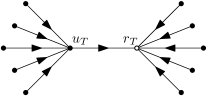
Figure 1. An orientation of a tree of diameter at most 3 towards a root $r_{T}$, which is not a leaf. The vertex $u_{T}$ is the only vertex distinct from $r_{T}$ with in-degree at least 1.

Consider some vertex $v$ which is a root in $i\geq 1$ trees of $\mathcal{T}$. Then $d^{+}(v)\leq\tfrac{k+1}{2}-i$ and thus $\delta(v)=2d^{+}(v)-k\leq 1-2i\leq-1$, with equality only if $i=1$. Hence, $\sum_{v\in D^{-}}\delta(v)\leq-|\mathcal{T}|$, with equality only if the roots $r_{T}$ are all distinct. Since $\sum_{v\in V(G)}\delta(v)=0$ and $\sum_{v\in D^{+}}\delta(v)=|D^{+}|$, we obtain $|\mathcal{T}|\leq|D^{+}|$, with equality only if the roots $r_{T}$ are pairwise distinct.

Each vertex $v\in D^{+}$ has positive in-degree, and thus $v$ is a non-root with in-degree at least 1 in at least one tree of $\mathcal{T}$. By the property of our orientation mentioned above (using the crucial fact that trees of $\mathcal{T}$ have diameter at most 3), recall that each tree $T$ of $\mathcal{T}$ contains at most one vertex of $D^{+}$ with in-degree at least one in $T$. It follows that $|\mathcal{T}|\geq|D^{+}|$, with equality only if each tree $T$ of $\mathcal{T}$ contains a unique vertex of $D^{+}$ with in-degree at least one in $T$. This shows that $|\mathcal{T}|=|D^{+}|$ and the equality implies that the roots $(r_{T})_{T\in\mathcal{T}}$ all distinct and each tree $T$ of $\mathcal{T}$ contains a different vertex of $D^{+}$ with in-degree at least one in $T$. Therefore, the function $T\in\mathcal{T}\mapsto u_{T}\in D^{+}$, where $u_{T}$ is the unique vertex of $D^{+}$ with in-degree at least 1 in $T$, is a bijection. Note that for every $T\in\mathcal{T}$, $u_{T}$ and $r_{T}$ are adjacent, and since the roots $r_{T}$ are pairwise distinct, the set of edges between $u_{T}$ and $r_{T}$, for $T\in\mathcal{T}$, forms a matching in $G^{c}$. Since $|\mathcal{T}|=|D^{+}|\geq\tfrac{n}{2}$, this matching is a perfect matching of $G^{c}$, a contradiction. ∎

We are now ready to prove Theorem 1.6.

Proof of 1.6..

By Theorem 1.5 and Lemma 6.2 it is sufficient to prove the upper bound. Assume that $G^{c}$ has an orientation with out-degree at most $d$, for some integer $d$. For every vertex $v\in V(G^{c})$, define $T_{v}$ to be the tree with root $v$ containing all the edges directed towards $v$. Then, $\bigcup_{v\in G^{c}}T_{v}=G^{c}$ and every vertex participates in at most $d+1$ trees. By 6.1, each of these trees is a co-interval graph, and thus $G$ has local boxicity at most $d$.

Assume first that $k$ is even. Then, $G^{c}$ has an Eulerian orientation, i.e. an orientation in which each vertex has out-degree $k/2$ and in-degree $k/2$, and the observation above implies that $G$ has local boxicity at most $k/2+1$, as desired.

If $k$ is odd, then $G^{c}$ has an orientation in which each vertex has out-degree at most $\tfrac{k+1}{2}$ (this can be seen by decomposing greedily $G^{c}$ into a union of edge-disjoint cycles and a forest, and finding an orientation with out-degree at most 1 of each of these graphs). The observation above then implies that $G$ has local boxicity at most $\tfrac{k+1}{2}+1=\tfrac{k+3}{2}$, which proves the theorem when $G^{c}$ has no perfect matching.

Finally, assume that $k$ is odd and $G^{c}$ contains some perfect matching $M$. Then, the graph obtained from $G^{c}$ by removing all the edges of $M$ has an Eulerian orientation. For each edge $uv\in M$, let $T_{uv}$ be the tree consisting of the edge $uv$ together with the edges oriented towards $u$, and the edges oriented towards $v$ (recall that $G^{c}$ has girth at least 5, so these edges induce a tree). Then, $\bigcup_{uv\in M}T_{uv}=G^{c}$, and every vertex participates in $\tfrac{k-1}{2}+1=\tfrac{k+1}{2}$ trees. By 6.1, each of these trees is a co-interval graph, and thus $G$ has local boxicity at most $\tfrac{k+1}{2}$, as desired. ∎

7. Proofs of Theorem 1.7 and Theorem 1.8

We will need the following two results (for the first one the exact constants are not given explicitly in [7] but can be easily deduced from their proof).

Theorem 7.1 ([7]).

Every graph with boxicity at most two and clique number at most $r$ has chromatic number at most $320r\log(2r)$.

Theorem 7.2 ([21]).

Every triangle-free graph with boxicity at most two has chromatic number at most 6.

We say that a graph of local boxicity at most 2 is of type $(1,1)$ if the graph has a 2-local box representation in which each box is local in at most one dimension distinct from the first dimension.

Lemma 7.3.

Let $G$ be a graph of type $(1,1)$ and clique number $\omega(G)=r$. Then $\chi(G)\leq 320r^{2}\log(2r)$. Moreover, if $r=2$, then $\chi(G)\leq 12$.

Proof.

Consider a $d$-dimensional 2-local box representation $(B_{v})_{v\in G}$ of $G$ such that each box is local in at most one dimension distinct from the first dimension. For each vertex $v$, let $I_{v}$ be the interval obtained by projecting $B_{v}$ on the first dimension. Let $G_{1}$ be the interval supergraph of $G$ associated to the intervals $(I_{v})_{v\in G}$. For every $2\leq i\leq d$, let $D_{i}$ be the set of vertices whose boxes are local in dimension $i$. Let $D_{1}=V(G)-\bigcup_{2\leq i\leq d}D_{i}$. Observe that $D_{1},\ldots,D_{d}$ form a partition of the vertex-set of $G$. For any $1\leq i\leq d$, let $\mathcal{P}_{i}$ be the family of connected components of $G_{1}[D_{i}]$, and let $\mathcal{P}=\bigcup_{1\leq i\leq d}\mathcal{P}_{i}$ (note that $\mathcal{P}$ forms a partition of $V(G)$).

For each set $S\in\mathcal{P}$, $G_{1}[S]$ is connected and thus the set $I_{S}=\bigcup_{v\in S}I_{v}$ is an interval. Let $H$ be the interval graph with vertex set $\mathcal{P}$ associated to the family of intervals $(I_{S})_{S\in\mathcal{P}}$. We claim that $H$ has clique number at most $r$. Indeed, suppose for the sake of contradiction that $r+1$ of the intervals $(I_{S})_{S\in\mathcal{P}}$ have non-empty intersection. Then there are $r+1$ vertices $v_{1},v_{2},\dots,v_{r+1}$ from different sets of $\mathcal{P}$, for which $\bigcap_{1\leq i\leq r+1}I_{v_{i}}\neq\varnothing$. Thus, the graph $G_{1}$ contains the complete graph on $v_{1},v_{2},\dots,v_{r+1}$. Note that if there is an edge in $G_{1}$ between two vertices $u,v$ lying in different sets $S_{u},S_{v}\in\mathcal{P}$, respectively, then the sets $S_{u}$ and $S_{v}$ do not lie in the same set $D_{i}$, and thus $u$ and $v$ are adjacent in $G$. This shows that every edge of $G_{1}$ between vertices from different sets of $\mathcal{P}$ also appears in $G$, which implies that $G$ contains a clique of size $r+1$, a contradiction. Hence, $H$ has clique number at most $r$, and since it is an interval graph, $\chi(H)\leq r$. Fix an $r$-coloring of $H$, and for each $S\in\mathcal{P}$, fix a coloring of $G[S]$ with at most $320r\log(2r)$ colors (such a coloring exists by Theorem 7.1 since $G[S]$ has boxicity at most 2).

We now assign to each vertex $v\in G$ a pair of colors as follows. Let $S\in\mathcal{P}$ be such that $v\in S$. Then, the first color assigned to $v$ is the color of $S\in V(H)=\mathcal{P}$ in the coloring of $H$, and the second color is the color of $v$ in $G[S]$. The total number of colors assigned is at most $r\cdot 320r\log(2r)=320r^{2}\log(2r)$. It remains to prove that this is a proper coloring of $G$. Let $uv$ be an edge of $G$. If $u$ and $v$ lie in the same set $S\in\mathcal{P}$, then since we have chosen a proper coloring of $G[S]$ the second colors of $u$ and $v$ are different. If $u$ and $v$ lie in different sets $S_{u},S_{v}$ of $\mathcal{P}$, then since $uv$ is also an edge of $G_{1}$, $S_{u}$ and $S_{v}$ are adjacent in $H$ and thus the first colors of $u$ and $v$ are different. This shows that $\chi(G)\leq 320r^{2}\log(2r)$.

Assume now that $r=2$. Then by Theorem 7.2 each graph $G[S]$ is 6-colorable, and thus $G$ itself has a coloring with at most $2\cdot 6=12$ colors, as desired. ∎

We are now ready to prove Theorem 1.8 and Theorem 1.7.

Proof of Theorem 1.8.

Let $(B_{v})_{v\in G}$ be a 2-local box representation of $G$ in some dimension $d$. We say that a vertex $v$ is local in dimension $i$ if its $d$-box $B_{v}$ is local in dimension $i$. If $G$ has local boxicity at most 1, it is the complete join of interval graphs, and since $G$ is triangle-free, this implies that $G$ itself is a (triangle-free) interval graph, and thus has chromatic number at most 2. So we can assume that some vertex $v$ is local in two different dimensions, say 1 and 2 without loss of generality. For any $1\leq i\leq d$, let $D_{i}$ be the set of vertices of $G$ that are local in dimension $i$. Note that $v\in D_{1}\cap D_{2}$, and $G[D_{1}\cap D_{2}]$ has boxicity at most 2, and thus $\chi(G[D_{1}\cap D_{2}])\leq 6$ by Theorem 7.2. This shows that if $V=D_{1}\cup D_{2}$, $\chi(G[V\setminus(D_{1}\triangle D_{2})])\leq 6$.

Note that all vertices of $V\setminus(D_{1}\cup D_{2})$ are neighbors of $v$, and therefore form an independent set in $G$. Since there is no pair of vertices $u\in D_{1}\cap D_{2}$ and $w\in V\setminus(D_{1}\cup D_{2})$ that are local in a common dimension, all vertices of $D_{1}\cap D_{2}$ are adjacent to all vertices of $V\setminus(D_{1}\cup D_{2})$. In particular, if $V\neq D_{1}\cup D_{2}$, the set $D_{1}\cap D_{2}$ is also an independent set in $G$. In this case we conclude that $\chi(G[V\setminus(D_{1}\triangle D_{2})])\leq 2$.

If $D_{2}\setminus D_{1}$ is an independent set, since $G[D_{1}]$ is of type $(1,1)$, it follows from Lemma 7.3 that $\chi(G)\leq\chi(G[D_{1}])+\chi(G[D_{2}\setminus D_{1}])+\chi(G[V\setminus(D_{1}\cup D_{2})])\leq 12+1+1=14$. The symmetric argument shows that if $D_{1}\setminus D_{2}$ is an independent set, then $\chi(G)\leq 14$. Consequently, we can assume that neither $D_{1}\setminus D_{2}$ nor $D_{2}\setminus D_{1}$ is an independent set, and in particular $G[D_{1}\setminus D_{2}]$ and $G[D_{2}\setminus D_{1}]$ both contain at least one edge. Fix $uw\in G[D_{1}\setminus D_{2}]$. We now consider two cases.

• Assume first that $u$ and $w$ are local together in a third dimension, say dimension 3 without loss of generality. Then, since $uw$ is not part of a triangle in $G$, $D_{2}\setminus D_{1}\subset D_{3}$. If $D_{1}\setminus D_{2}\not\subseteq D_{3}$, without loss of generality there is a vertex in $D_{1}\setminus(D_{2}\cup D_{3})$, and this vertex is adjacent to every vertex in $D_{2}\cap D_{3}=D_{2}\setminus D_{1}$. Thus, $D_{2}\setminus D_{1}$ is an independent set, which contradicts our assumption above. Hence, we can assume that $D_{1}\setminus D_{2}\subseteq D_{3}$, and thus $D_{1}\triangle D_{2}\subseteq D_{3}$. Since $G[D_{3}]$ is of type $(1,1)$ it follows from Lemma 7.3 and the discusion above that

  $$\chi(G)\leq\chi(G[D_{1}\triangle D_{2}])+\chi(G[V\setminus(D_{1}\triangle D_{2})])\leq 12+6=18.$$

• We can now assume without loss of generality that $u\in D_{3}$ and $w\in D_{4}$. Note that in this case $D_{3}\neq D_{1}$ and $D_{4}\neq D_{1}$. Then, since $uw$ is not part of a triangle in $G$, $D_{2}\setminus D_{1}\subset D_{3}\cup D_{4}$. Moreover, if $D_{1}\setminus D_{2}\not\subseteq D_{3}\cup D_{4}$, then there is a vertex $w\in D_{1}\setminus(D_{2}\cup D_{3}\cup D_{4})$, which is connected to every vertex in $D_{2}\setminus D_{1}$, and therefore $D_{2}\setminus D_{1}$ is an independent set, contradicting our assumption. Thus, $D_{1}\triangle D_{2}\subseteq D_{3}\cup D_{4}$. Note that if $D_{3}\cap D_{2}=\varnothing$ or $D_{4}\cap D_{2}=\varnothing$, then all vertices of $D_{2}\setminus D_{1}$ are adjacent to $u$, or all are adjacent to $w$, respectively. In both cases we obtain that $D_{2}\setminus D_{1}$ is an independent set, a contradiction. This shows that $D_{2}\cap D_{3}\neq\varnothing$ and $D_{2}\cap D_{4}\neq\varnothing$. Since $G[D_{1}\cap D_{3},D_{2}\cap D_{4}]$ and $G[D_{1}\cap D_{4},D_{2}\cap D_{3}]$ are complete bipartite graphs, each of $D_{1}\cap D_{3},D_{1}\cap D_{4},D_{2}\cap D_{3}$ and $D_{2}\cap D_{4}$ is an independent set. Since $D_{1}\triangle D_{2}\subseteq D_{3}\cup D_{4}$, this shows that $G[D_{1}\triangle D_{2}]$ is 4-colorable. Thus,

  $$\chi(G)\leq\chi(G[D_{1}\triangle D_{2}])+\chi(G[V\setminus D_{1}\triangle D_{2}])\leq 4+6=10.$$

This concludes the proof of the theorem.∎

In the proof of Theorem 1.7 we made no effort to optimize the multiplicative constant.

Proof of Theorem 1.7.

We will prove by induction on $r\geq 2$ that any graph of local boxicity at most 2 and clique number at most $r$ has chromatic number at most $320r^{3}\log(2r)$. The claim holds for $r=2$ by Theorem 1.8. Suppose now that $r\geq 3$ and the property holds for $r-1$. Let $G=(V,E)$ be a graph of local boxicity at most 2 and clique number at most $r$, and let $(B_{v})_{v\in G}$ be a 2-local box representation of $G$ in some dimension. If $G$ has local boxicity at most 1, then $G$ is the complete join of interval graphs, and thus $\chi(G)=\omega(G)=r$, so we can assume that some box $B_{v}$ is local in two dimensions, say in dimensions 1 and 2 without loss of generality. For $i=1,2$, let $D_{i}$ be the set of vertices whose boxes are local in dimension $i$ (and note that $v\in D_{1}\cap D_{2}$). As all the vertices of $V\setminus(D_{1}\cup D_{2})$ are neighbors of $v$, the graph $G[V\setminus(D_{1}\cup D_{2})]$ has clique number at most $r-1$, and by the induction hypothesis it has a coloring with at most $320(r-1)^{3}\log(2(r-1))\leq 320(r-1)^{3}\log(2r)$ colors. Each of $G[D_{1}]$ and $G[D_{2}]$ is of type $(1,1)$ and thus both $G[D_{1}]$ and $G[D_{2}\setminus D_{1}]$ have a coloring with at most $320r^{2}\log(2r)$ by Lemma 7.3. It follows that $G$ has a coloring with at most

$$320(r-1)^{3}\log(2r)+2\cdot 320r^{2}\log(2r)\leq 320r^{3}\log(2r)$$

colors, as desired. ∎

8. Conclusion and open problems

Two natural problems are to close the gap between the lower bound of $\Omega(\sqrt{m}/\log m)$ and the upper bound of $O(\sqrt{m})$ for graphs with $m$ edges, and the lower bound of $\Omega(\sqrt{g}/\log g)$ and the upper bound of $O(\sqrt{g})$ for graphs of Euler genus $g$.

We have proved that the family of graphs of local boxicity at most 2 is $\chi$-bounded, which extends a classical result on graphs with boxicity at most 2. It was proved in [24] that if $G$ is the complement of a graph of boxicity at most 2, then $\chi(G)=O(\omega(G)\log\omega(G))$, and thus the family of complements of graphs of boxicity at most 2 is $\chi$-bounded. A natural question is whether this extends to the family of complements of graphs of local boxicity at most 2.

Question 1.

Is the family $\{G^{c}\,|\,\mathrm{lbox}(G)\leq 2\}$ $\chi$-bounded?

It was observed by James Davies (personal communication) that the answer to this question is negative. Given an integer $n\geq 2$, the shift graph $S_{n}$ is the graph whose vertices are the ordered pairs $(i,j)$ with $1\leq i<j\leq n$, with an edge between $(i,j)$ and $(k,\ell)$ if and only if $j=k$ or $\ell=i$. It can be checked that $S_{n}$ is triangle-free, and Erdős and Hajnal [14] proved that for any $n\geq 2$, $\chi(S_{n})=\lceil\log n\rceil$. James Davies noted that the complement of $S_{n}$ has local boxicity at most 2: to see this, map each pair $(i,j)$ to the $n$-dimensional box whose projection is equal to $\{0\}$ in dimension $i$, $\{1\}$ in dimension $j$, and $\mathbb{R}$ in the other dimensions. This shows that the family of triangle-free graphs in $\{G^{c}\,|\,\mathrm{lbox}(G)\leq 2\}$ has unbounded chromatic number, and thus 1 has a negative answer.

Recent development. After we made our manuscript public, the authors of [28] improved their bound on the local boxicity of graphs of maximum degree $\Delta$ to $O(\Delta)$, matching the bound of Theorem 1.1 (and as a consequence, also matching the bound of Theorem 1.2). Their proof avoids the use of number theoretic tools altogether.

Acknowledgments.

The authors would like to thank Matěj Stehlík for interesting discussions and for suggesting to investigate the chromatic number of graphs of local boxicity at most 2 and their complements. We are also grateful to James Davies for allowing us to present his negative answer to 1, and to Bartosz Walczak for giving us the correct constant in Theorem 7.1.

References

- [1] A. Adiga, D. Bhowmick, and L. S. Chandran. Boxicity and poset dimension. SIAM Journal on Discrete Mathematics, 25(4):1687–1698, 2011.
- [2] A. Adiga and L. S. Chandran. Representing a cubic graph as the intersection graph of axis-parallel boxes in three dimensions. SIAM Journal on Discrete Mathematics, 28(3):1515–1539, 2014.
- [3] A. Adiga, L. S. Chandran, and N. Sivadasan, Lower bounds for boxicity, Combinatorica, 34:631–655, 2014.
- [4] R. C. Baker, G. Harman, and J. Pintz. The difference between consecutive primes, II. Proceedings of the London Mathematical Society, 83(3):532–562, 2001.
- [5] T. Bläsius, P. Stumpf, and T. Ueckerdt. Local and union boxicity. Discrete Mathematics, 341(5):1307–1315, 2018.
- [6] J. P. Burling. On coloring problems of families of prototypes (PhD thesis). University of Colorado, Boulder, 1965.
- [7] P. Chalermsook and B. Walczak. Coloring and maximum weight independent set of rectangles. In: ACM-SIAM Symposium on Discrete Algorithms (SODA), 2021.
- [8] L. S. Chandran, M. C. Francis, and N. Sivadasan. Boxicity and maximum degree. Journal of Combinatorial Theory, Series B, 98(2):443–445, 2008.
- [9] V. Costa, S. Dantas, and D. Rautenbach. Matchings in graphs of odd regularity and girth. Discrete Mathematics, 313(24):2895–2902, 2013.
- [10] G. Damásdi, S. Felsner, A. Girão, B. Keszegh, D. Lewis, D. T. Nagy, and T. Ueckerdt. On covering numbers, young diagrams, and the local dimension of posets. SIAM Journal on Discrete Mathematics, 35(2):915–927, 2021.
- [11] P. Dusart. Autour de la fonction qui compte le nombre de nombres premiers, Manuscript, 1998.
- [12] P. Dusart. Estimates of some functions over primes without R.H. arXiv preprint arXiv:1002.0442, 2010.
- [13] P. Dusart. Explicit estimates of some functions over primes. The Ramanujan Journal, 45(1):227–251, 2018.
- [14] P. Erdős and A. Hajnal. Some remarks on set theory. IX. Combinatorial problems in measure theory and set theory. Michigan Math. J., 11:107–127, 1964.
- [15] P. Erdős, H. A. Kierstead, and W. T. Trotter. The dimension of random ordered sets. Random Structures & Algorithms, 2(3):253–275, 1991.
- [16] P. Erdős and L. Lovász. Problems and results on 3-chromatic hypergraphs and some related questions, 1973. In Colloq. Math. Soc. János Bolyai, volume 10, 1975.
- [17] L. Esperet. Boxicity of graphs with bounded degree. European Journal of Combinatorics, 30(5):1277–1280, 2009.
- [18] L. Esperet. Boxicity and topological invariants. European Journal of Combinatorics, 51:495–499, 2016.
- [19] A. D. Flaxman and S. Hoory. Maximum matchings in regular graphs of high girth. The Electronic Journal of Combinatorics, 14, #N1, 2007.
- [20] A. Frieze and M. Karoński. Introduction to random graphs. Cambridge University Press, 2016.
- [21] B. Grünbaum and E. Asplund. On a coloring problem. Mathematica Scandinavica, 8:181–188, 1960.
- [22] C. Hendler. Schranken für Färbungs-und Cliquenüberdeckungszahl geometrisch repräsentierbarer Graphen. PhD thesis, 1998.
- [23] S. Janson, T. Łuczak, and A. Ruciński. Random Graphs. Wiley, 2000.
- [24] Gy. Károlyi. On point covers of parallel rectangles. Periodica Mathematica Hungarica, 23:105–107, 1991.
- [25] J. Kim, R. R. Martin, T. Masařík, W. Shull, H. C. Smith, A. Uzzell, and Z. Wang. On difference graphs and the local dimension of posets. European Journal of Combinatorics, 86:103074, 2020.
- [26] K. Knauer and T. Ueckerdt. Three ways to cover a graph. Discrete Mathematics, 339(2):745–758, 2016.
- [27] A. Liebenau and N. Wormald. Asymptotic enumeration of graphs by degree sequence, and the degree sequence of a random graph. arXiv preprint arXiv:1702.08373, 2017.
- [28] A. Majumder and R. Mathew. Local boxicity, local dimension, and maximum degree. arXiv preprint arXiv:1810.02963v2, 2019.
- [29] M. Mitzenmacher and E. Upfal. Probability and computing: Randomization and probabilistic techniques in algorithms and data analysis. Cambridge university press, 2017.
- [30] M. Molloy and B. Reed. Graph colouring and the probabilistic method, volume 23. Springer Science & Business Media, 2013.
- [31] F. S. Roberts. Recent progresses in combinatorics, chapter on the boxicity and cubicity of a graph, 1969.
- [32] A. Scott and P. Seymour. A survey of -boundedness. Journal of Graph Theory, 95(3):473–504, 2020.
- [33] A. Scott and D. Wood. Better bounds for poset dimension and boxicity. Transactions of the American Mathematical Society, 373(3):2157–2172, 2020.
- [34] C. Thomassen. Interval representations of planar graphs. Journal of Combinatorial Theory, Series B, 40(1):9–20, 1986.