Scaling of non-adiabaticity in disordered quench of quantum Rabi model close to phase transition

Abstract

Dynamics of a system exhibits non-adiabaticity even for slow quenches near critical points. We analyze the response to disorder in quenches on a non-adiabaticity quantifier for the quantum Rabi model, which possesses a phase transition between normal and superradiant phases. We consider a disordered version of a quench in the Rabi model, in which the system residing in the ground state of an initial Hamiltonian of the normal phase is quenched to the final Hamiltonian corresponding to the critical point. The disorder is inserted either in the total time the quench or in the quench parameter itself. We solve the corresponding quantum dynamics numerically, and find that the non-adiabatic effects are unaffected by the presence of disorder in the total time of the quench. This result is then independently confirmed by the application of adiabatic perturbation theory and the Kibble-Zurek mechanism. For the disorder in the quench parameter, we report a monotonic increase in the adiabaticity with the strength of the disorder. Lastly, we consider a quench where the final Hamiltonian is chosen as the average over the disordered final Hamiltonians, and show that this quench is more adiabatic than the average of the quenches with the disorder in final Hamiltonian.

I Introduction

Dynamics of quantum systems lead to many phenomena of fundamental importance in non-equilibrium physics meyer96 ; amico08 ; misbah10 ; silva'11 ; zudov12 ; eisert'15 . Recent advancements in the experiments have provided controlled implementation of dynamics in physical systems, like in cold atoms Schreiber15 ; Bordia16 ; Choi16 ; Bordia17a ; Bordia17b and ion-traps Smith16 ; Martinez16 ; Neyenhuis17 ; Zhang17 . Inspecting the dynamics of quantum systems is crucial for technological advancements too, e.g., for modelling quantum simulators Lew07 ; Buluta09 ; Lew12 ; Nori14 and adiabatic quantum computations Cirac12 ; Lidar18 . Dynamics of physical systems possessing a quantum phase transition (QPT) has always been an interesting area of research Heyl13 ; Biroli11 ; Biroli13 ; Gambassi11 ; Silva15 ; Silva16 ; Heyl18 ; Halimeh18 ; Dutta18 ; Haldar20 ; Sehrawat20 . One striking feature of dynamics of a physical system near a critical point is that adiabaticity Born28 cannot be maintained due to a vanishing energy gap sachdev'11 .

Quantum Rabi model (QRM), a simplified version of the Dicke model dicke'54 , with only one two-level atom interacting with a quantized cavity field, exhibits a QPT from a normal phase to a superradiant phase when the ratio of atomic transition frequency to the cavity field frequency goes to infinity bishop'96 ; bishop'01 ; levine'04 ; hines'04 ; feshke'12 ; nori'10 ; choi'10 ; ashhab'13 ; plenio'15 . Thus in this case, the infinite ratio of frequencies plays the role of the thermodynamic limit in usual phase transitions. Recently, it has also been shown that the QPT in the QRM, as well as the dynamics near the QPT, can be experimentally probed in the setting of a single trapped ion plenio'17 . In plenio'15 , a quench dynamics of the system described by a QRM in the normal phase is considered, and the non-adiabatic effect with respect to the rate of the quench is investigated. For sufficiently slow quenches, a measure of degree of non-adiabaticity of a quench, the residual energy, follows a power-law scaling with the quench rate. For quenches ending away from the critical point, the fall in residual energy is sharper than for the quench ending at the critical point. For slow enough quenches, the ideas of adiabatic perturbation theory (APT) grandi'10 and the Kibble-Zurek mechanism (KZM) kibble'76 ; zurek'85 ; zurek'96 ; zurek'97 ; dziar'10 ; zurek'14 can be applied to obtain the scaling of residual energy with respect to the rate of quench. The KZM was initially developed to describe formation of the universe, and later on applied to condensed matter systems. It predicts formation of defects when the system is driven through a symmetry breaking phase transition. It has been successfully applied to various models possessing phase transitions dicke'54 ; lipkin'65 ; botet'82 ; botet'83 ; polko'05 ; zurek'05 ; dziar'05 ; damski'05 ; damski'06 ; damski'07 ; damski'08 ; niko'16 .

In real circumstances, the system parameters and the devices controlling the tuning of these parameters may not be ideal. In such scenarios, it is important from an experimentalist’s point of view to know about the “average” behavior of relevant physical quantities. In this article, we study the quench dynamics in the QRM in presence of a disorder in the quench parameters. The aim is to analyze the (quenched) average non-adiabatic effects of the dynamics, affected by quenched disorder. Ideally, the system residing in the ground state of the Hamiltonian in the normal phase is linearly quenched to a final Hamiltonian corresponding to the critical point of the QPT. We analyze disordered versions of the above quench in the following two cases. In the first case, the disorder is present in the total quench time, whereas in the second case, there is disorder in the quench parameter.

In both the cases, we study the average residual energy, where the average is taken over all disordered quenches. For the first case, we find that the quenched average residual energy scales similarly as the residual energy for the ordered quench, with respect to the rate of the ordered quench. Therefore, the non-adiabaticity for quenches ending at the critical point, is unaffected by the disorder in the rate of quench. For sufficiently slow quenches, we also apply APT and KZM to obtain the same result, which indicates the applicability of KZM even to disordered quenches. For the second case of disordered quench, we report a monotonic increase in the adiabatic nature of the quench with the strength of the disorder. Furthermore, we also consider a quench where the final Hamiltonian is chosen as average over disordered final Hamiltonians. We show that this quench is “more adiabatic” than the quenches with the disordered final Hamiltonians.

The rest of the paper is organized as follows. In sec. II, we discuss the prerequisites, and is subdivided into three subsections. We start with briefly reviewing QPT in the QRM in subsec. II.1. In subsec. II.2, dynamics of the QRM and a measure of non-adiabaticity of the quench is discussed, and in subsec. II.3, quenched averaging of physical quantities over the disorder is briefly explained. In sec. III, we study a quench of the system from a given initial Hamiltonian to the critical point, but with a disorder in the rate of quench. For sufficiently slow quenches, we use APT and KZM to reproduce the scaling exponents in subsec. III.1. In sec. IV, we study a disordered quench of the system from a given initial Hamiltonian to a disordered Hamiltonian which do not correspond to the critical point Hamiltonian. We present a conclusion in sec. V.

II Prerequisites

II.1 Quantum Rabi model

We briefly discuss here about a quantum phase transition in quantum Rabi model. A two-level atom in the presence of quantized cavity field can be modelled by the quantum Rabi Hamiltonian, which has the form

$$H_{Rabi}=\hslash\Big{[}\omega a^{\dagger}a+\frac{\Omega}{2}\sigma_{z}-\lambda(a^{\dagger}+a)\sigma_{x}\Big{]},$$ (1)

where $\hslash$ is the reduced Planck’s constant, $\omega$ is the frequency of the cavity field, $\Omega$ is the atomic transition frequency, $\lambda$ is the coupling coefficient, $\sigma_{x,y,z}$ are the usual Pauli operators, and $a$ and $a^{\dagger}$ are respectively the annihilation and creation operators of cavity field. Exact solutions to quantum Rabi Hamiltonian are devoid of any closed form, despite it being solvable braak . It is shown in plenio'15 that an effective Hamiltonian describing low energy physics of $H_{Rabi}$ can be deduced for $\frac{\Omega}{\omega}\gg 1.$ In fact, in the limit $\frac{\Omega}{\omega},\frac{\lambda}{\omega}\to\infty$, $H_{Rabi}$ undergoes a quantum phase transition, which can be shown using its effective low energy Hamiltonian plenio'15 .

The effective low energy Hamiltonian for $H_{Rabi}$ in the limit $\frac{\Omega}{\omega}\to\infty$ is given by

$$H_{np} =\hslash\Big{[}\omega a^{\dagger}a-\frac{\omega g^{2}}{4}(a^{\dagger}+a)^{2}-\frac{\Omega}{2}\Big{]};\text{ }\left|g\right|\leqslant 1,$$ (2)

$$H_{sp} =\hslash\Big{[}\omega a^{\dagger}a-\frac{\omega}{4g^{4}}(a^{\dagger}+a)^{2}-\frac{\Omega}{4}(g^{2}+g^{-2})\Big{]};\text{ }\left|g\right|>1,$$

where $g=\frac{2\lambda}{\sqrt{\Omega\omega}}$ is a dimensionless parameter and quantum phase transitions occur at $|g|=1$. Subscripts $np$ in $H_{np}$ and $sp$ in $H_{sp}$ stands for normal ($|g|\leqslant 1$) and superradiant ($|g|>1$) phases, respectively. In order to obtain the low energy effective Hamiltonians from $H_{Rabi}$ in the limit $\frac{\Omega}{\omega}\to\infty$, certain unitary transformations are applied such that the low energy spectrum of $H_{Rabi}$, corresponds to one of the spin subspaces. Then a projection of $H_{Rabi}$ on that spin subspace provides the effective Hamiltonians plenio'15 .

II.2 Linearly quenched dynamics in normal phase

In this subsection, we briefly present the quench dynamics of the system, prepared initially in its ground state, with a linearly quenched time-dependent Hamiltonian in the normal phase plenio'15 . Let $g$ be the quench parameter and have the form

$$g(t)=\frac{g_{f}}{\tau}t;\hskip 14.22636pt0\leq t\leq\tau.$$ (3)

The dynamics starts at time $t=0$ with $g=0$, and ends at time $t=\tau$ with $g=g_{f}$. Here, $g_{f}$ is the final value of the quench parameter, $g$, and $\tau$ is the total time of quench. Note that $g_{f}\leq 1$ for system to be in normal phase and $\tau$ controls the rate of the quench from $g=0$ to $g_{f}$. Larger the values of $\tau$, the slower is the rate of the quench. It is known generically that the evolution of any system, if it is always gapped, can be adiabatic if the quench rate is sufficiently slow. But for a dynamics very close to a critical point, adiabaticity breaks even for very slow quenches. To capture the non-adiabaticity of such dynamics, let us consider a quantity called the residual energy, given by

$$E_{r}(\tau)=\langle\Psi(\tau)|H_{np}(g(\tau))|\Psi(\tau)\rangle-E_{G}(\tau),$$ (4)

where $|\Psi(t)\rangle$ is the wavefunction of the system at time $t$ and $E_{G}(t)$ is the ground state of instantaneous Hamiltonian $H_{np}(t)$.

Solving the dynamics for Hamiltonian $H_{np}(g(t))$ (using equation of motion in the Heisenberg picture), reduces to solving the following differential equations plenio'15

$$\frac{i}{\omega}\frac{du(t)}{dt}=\left(1-\frac{g^{2}(t)}{2}\right)u(t)-\frac{g^{2}(t)}{2}v(t),$$

$$-\frac{i}{\omega}\frac{dv(t)}{dt}=\left(1-\frac{g^{2}(t)}{2}\right)v(t)-\frac{g^{2}(t)}{2}u(t),$$ (5)

with initial conditions $u(0)=1$ and $v(0)=0$, and the constraint $|u(t)|^{2}-|v(t)|^{2}=1$. And the residual energy is then given in terms of $u(t)$ and $v(t)$ as

$$E_{r}(\tau)=\hslash\left(\omega|v(\tau)|^{2}-\frac{\omega^{2}g_{f}}{4}|u(\tau)+v(\tau)|^{2}-\frac{\omega\left(\sqrt{1-g_{f}^{2}}-1\right)}{2}\right).$$ (6)

It has been shown that for very $slow$ quenches ($\omega\tau\gg 1$), $E_{r}$ scales with total time of quench, $\tau$, maintaining a power law. For quenches ending far away from the critical point, i.e., $g_{f}\ll 1$, $E_{r}\propto\tau^{-2}$, whereas for quenches ending near the critical point, i.e., $g_{f}\sim 1$, $E_{r}\propto\tau^{\frac{-1}{3}}$ plenio'15 . The scaling exponent makes transition from -2 to $\frac{-1}{3}$ as the end point of quench moves towards the critical point, when the excitations in the system starts to be appreciable (i.e., adiabaticity breaks).

II.3 Quenched averaging

In real experiments, inaccuracies invariably creep in. Therefore, it becomes important to look out for a quantity of interest under such scenarios. In this paper, our aim is to study quantities affected by disorder in a quench dynamics of the system. The relevant quantities of interest are therefore disorder averaged quantities. However, the type of averaging depends on the strain of the disorder. Consider $O$ to be an observable of interest for a given quench dynamics of the system. And let $\delta$ be a parameter, which brings in disorder for a given single run of the quench dynamics, and the corresponding probability distribution is given by $p(\delta)$. Let the disorder-affected observable be given by $O_{\delta}$. Then, if the disorder in $\delta$ is of the quenched type, viz. if the equilibration time of the disorder is much larger than the time required for all the relevant observations about the observable $O$, then the quantity of interest for an experimentalist will be the quenched average of $O$, which is given by

$$\overline{O}=\frac{1}{[\delta]}\sum_{\delta}O_{\delta},$$ (7)

where the sum runs over all realizations of the disorder, obeying the distribution $p(\delta)$, for different runs of the experiment, and $[\delta]$ is the number of runs of the experiment. One of course needs to perform a convergence check using a higher number of runs of the experiment.

III Dynamics with disorder in total time of quench

In this section, we consider a disorder in the rate of the quench, i.e., in the total time of quench. We study the effect of disorder on the scaling of the disorder averaged residual energy, $\overline{E}_{r}$, with respect to the quench time, $\tau$, of the quench in the ordered case. We consider a quench where the system starts in the normal phase ($\frac{\Omega}{\omega}\to\infty$ and $|g|<1$) and approaches the critical point ($g=1$) linearly. We consider the initial wave function of the system to be the ground state of $H_{np}(g=0)$ followed by the quench,

$$g(t)=\frac{1}{\tau_{\delta}}t;\hskip 14.22636pt0\leq t\leq\tau_{\delta}=\tau(1+\delta),$$ (8)

where $\tau$ is the total quench time in the absence of disorder, $\tau_{\delta}$ is the total quench time in the disordered case, with $\delta$ being the disordered parameter. Now, we assume that $\delta$ is a number chosen from a distribution, $p(\delta)$, which is given as

$$p(\delta) = \frac{\exp\left(\frac{-\delta^{2}}{2\sigma^{2}}\right)}{\sqrt{2\pi}\sigma\text{erf}\left(\frac{3}{\sqrt{2}}\right)};\hskip 14.22636pt|\delta|\leq 3\sigma,$$

$$p(\delta) = 0;\hskip 71.13188pt\text{otherwise,}$$ (9)

where $\mbox{erf}(\cdot)$ is the Gauss error function. The probability distribution is very close to the ubiquitous Gaussian distribution. The reason for choosing such a distribution, instead of the usual Gaussian, is that $\tau_{\delta}$ cannot be negative, which implies that $\delta$ cannot be less than -1. With the chosen distribution, this is achieved by choosing $\sigma$ in the range $[0,\frac{1}{3}]$. Note that $\sigma$ is no more the standard deviation of the distribution $p(\delta)$, but it can still be seen as a measure of dispersion.

Solving the equation of motion in Heisenberg picture numerically, we observe that for slow quenches $(\omega\tau\gg 1)$, the disorder averaged residual energy follows a power law fall with respect to the quench time $\tau$, i.e., $\overline{E}_{r}\propto\tau^{\nu}$, with $\nu$ remaining close to $-\frac{1}{3}$, whatever be the $\sigma$, in the range $\left[0,\frac{1}{3}\right]$. This suggest that the scaling is robust against the disorder present in total quench time. We give the scaling exponents, $\nu$, for the scaling relation $\overline{E}_{r}\propto\tau^{\nu}$, with varying dispersion of the disorder distribution in Table 1. It can be seen that as $\sigma$ increases, there is no change in the scaling exponent $\nu$, correct to the third decimal place, it is still $-\frac{1}{3}$.

Table 1: Response to disorder in quench time on scaling exponent of non-adiabaticity. We tabulate here the scaling exponents of the disorder averaged residual energy, $\overline{E}_{r}$, with the total time of ordered quench, $\tau$, for different dispersions of the disorder distribution. The results are obtained by solving the Eq. (II.2) numerically. Our precision enables us to predict only up to three significant figures. Within this precision, the scalings remain unchanged with change of the disorder strength, as quantified by the dispersion, $\sigma$. Compare this with the variation in the scalings in the next table. All quantities in the table are dimensionless.

Dispersion	Scaling exponent
$\sigma$	$\nu$
0.01	-0.333
0.1	-0.333
0.2	-0.333
0.3	-0.333
0.33	-0.333

III.1 Scaling exponents within adiabatic perturbation theory and Kibble-Zurek mechanism

Adiabatic perturbation theory (APT) is a useful method to solve the dynamics of a system going through a very slow quench grandi'10 . For a quench given in Eq. (3), with $g_{f}\ll 1$ and $\omega\tau\gg 1$ (slow quench), it has been shown that the residual energy, within APT, behaves as plenio'15

$$E_{r}(\tau)\approx\frac{\hslash g^{4}_{f}}{16\omega(1-g^{2}_{f})^{\frac{5}{2}}}\tau^{-2}.$$ (10)

But APT fails when the system has a vanishing energy gap during the dynamics, even for slow quenches. Therefore, for a quench with $g_{f}\sim 1$, the scaling given by Eq. (10) is no more correct. In such cases, the KZM can be used, and it was shown in plenio'15 that for $g_{f}\sim 1$, the scaling exponents within KZM come out to be $-\frac{1}{3}$, just as obtained numerically from the equation of motion in the Heisenberg picture directly.

In this subsection, our aim is to verify whether for disordered systems, scalings predicted by KZM matches with that obtained directly from the Heisenberg equation of motion (as already presented in Table 1). Consider, therefore, the quench given in Eq. (8). The basic idea of KZM is to split a dynamics into adiabatic and impulsive regimes based on a comparison of two time scales dziar'10 ; zurek'14 ; damski'08 ; plenio'17 . The first of these time scales is the “relaxation time” of the system, which is inversely proportional to the energy gap ($\eta$) between the ground state and the first allowed excited state zurek'05 . Precisely, it is $\hslash\eta^{-1}$, where $\eta=2\hslash\omega\sqrt{1-g^{2}}$. The relaxation time of the system is the time required by the system to respond to a given quench. And the second one, which is known as the “transition time” damski'07 , is the time scale in which there occurs changes in the Hamiltonian, and is characterized by $|\eta/\dot{\eta}|$. If the relaxation time is lower than the transition time, the dynamics of the system is in the adiabatic regime, but otherwise, the dynamics is in the impulsive regime and the system stops to react to the quench.

Let the value of the quench parameter which splits the adiabatic and impulsive regimes be given by $g=\hat{g}$, which can be obtained using

$$\left|\frac{\eta(\hat{g})}{\dot{\eta}(\hat{g})}\right|=\frac{\hslash}{\eta(\hat{g})},$$ (11)

whence we get

$$\frac{(1-\hat{g}^{2})^{3/2}}{\hat{g}}=\frac{1}{2\omega\tau_{\delta}}.$$ (12)

Note that for $\sigma\in[0,0.33]$ (range taken in Table 1), for the distribution given in Eq. (III), $\delta$ is never closer enough to -1, so that $(1+\delta)^{-1}$ blows up. Therefore, for a slow quench ($\omega\tau\gg 1$) and a smaller enough dispersion $\sigma$, $\omega\tau_{\delta}\gg 1$, too. This implies that the R.H.S. of Eq. (11) is close to zero, and L.H.S. is close to zero when $\hat{g}\approx 1$, whereby we can write $\hat{g}=1-\hat{\epsilon}$, for a small positive $\hat{\epsilon}$. Ignoring higher than linear order in $\hat{\epsilon}$, we obtain $\hat{\epsilon}\approx 1/(2/3+2^{5/3}(\omega\tau_{\delta})^{2/3})$, and because $\omega\tau_{\delta}\gg 1$, we get

$$\hat{g}\approx 1-\frac{1}{2^{5/2}(\omega\tau_{\delta})^{2/3}}.$$ (13)

Since $\hat{g}\lesssim 1$, and the system freezes at $g=\hat{g}$, therefore, $E_{r}(\tau_{\delta})\approx E_{r}(\hat{g})$, where $E_{r}(\hat{g})$ is the residual energy when $g=\hat{g}$. Now, it can be shown using APT that for slow quenches $(\omega\tau_{\delta}\gg 1)$, the residual energy, $E_{r}(\hat{g})$, is given by

$$E_{r}(\hat{g})\approx\frac{\hslash\hat{g}^{2}}{16\omega(1-\hat{g}^{2})^{5/2}}\tau^{-2}_{\delta},$$ (14)

which, using relations (12) and (13), can be expressed as

$$E_{r}(\hat{g})\approx\frac{\hslash\omega}{4\sqrt[3]{2}(\omega\tau)^{\frac{1}{3}}}\left[(1+\delta)^{-\frac{1}{3}}-\frac{(1+\delta)^{-1}}{12\sqrt{2}(\omega\tau)^{\frac{2}{3}}}\right].$$ (15)

The disorder averaged residual energy, at the end of the quench, is given as $\overline{E}_{r}=\int E_{r}(\hat{g})p(\delta)d\delta$. Now, the integrals of $(1+\delta)^{-1/3}p(\delta)$ and $(1+\delta)^{-1}p(\delta)$ are of the order of 1, for $\sigma<0.33$. Therefore the disorder averaged residual energy for low values of $\sigma$ is

$$\overline{E}_{r}\approx\frac{\hslash\omega}{4\sqrt[3]{2}}(\omega\tau)^{-1/3}.$$ (16)

Note that the second term in the expression of $\overline{E}_{r}$ is dropped because of the slow quench, i.e., $\omega\tau\gg 1$. Therefore the scaling exponent obtained using APT and KZM is $\nu=-\frac{1}{3}$, which matches with the numerically obtained data by directly solving the equation of motion in the Heisenberg picture, as presented in Table 1. Thus, both the analytical but approximate calculation using APT and KZM as well as the numerical but exact calculation provide the same scaling for the averaged residual energy in the disordered dynamics in which quench stops at the critical point of the ordered quantum Rabi model, and matches with the scaling obtained in the ordered case. The disorder considered is of quenched type and is inserted in the total time of quench. We will now investigate the outcome of insertion of disorder in the final value of the quench parameter.

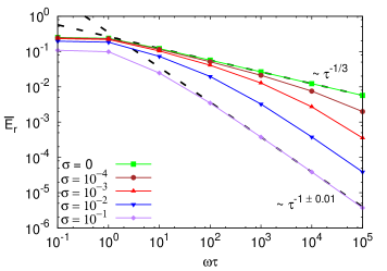
Figure 1: Analyzing adiabaticity in disordered quenches in the quantum Rabi model. The disorder averaged residual energy, $\overline{E}_{r}$, is plotted against $\omega\tau$ of a disordered quench (given in Eq. (17)). For slow quenches $(\omega\tau\gg 1)$ and small standard deviation ($\sigma$) of the disorder, $\overline{E}_{r}$ maintains a power-law scaling with the total time of quench, $\tau$, of the corresponding ordered quench. As $\sigma$ shifts from 0 to 0.1, the scaling exponent shifts from $-\frac{1}{3}$ to $-1\pm 0.01$. For the trend of the scalings with varying $\sigma$, see also Table 2. The degrees of adiabaticity of the quenches increase with the increase in strength of the disorder, as quantified by the standard deviation, $\sigma$, of the disorder. $\overline{E}_{r}$ is plotted in the units of $\hslash\omega$ and $\omega\tau$ is dimensionless.

IV Dynamics with disorder in quench parameter

In this section, we consider the quench given in Eq. (3) with the disorder in the final Hamiltonian, i.e., the final value of the quench parameter, $g$. The disorder is chosen in such a way that it offers resistance to the quench to end at the critical point (while “approaching” from the left, i.e. over lower values), and thus the disordered final value of quench parameter, $g$, is given by

$$g_{f}(\delta)=(1-|\delta|),$$

where, in this case, the disorder parameter, $\delta$, is chosen from a quenched Gaussian distribution of mean zero and standard deviation, $\sigma$. Therefore the quench is given by

$$g(t)=\frac{g_{f}(\delta)}{\tau}t;\hskip 28.45274pt0\leq t\leq\tau.$$ (17)

Also, $\sigma$ is taken in the range $[0,~{}0.1]$, resulting in the system to have $g(t)>0$ satisfied with very high probability. We numerically obtain the disorder averaged residual energy, $\overline{E}_{r}$, and plot it in the units of $\hslash\omega$, with respect to $\omega\tau$, in Fig. 1. It is known that for the case with no disorder, i.e., $\sigma=0$, $\overline{E}_{r}\propto\tau^{-\frac{1}{3}}$, for higher values of $\omega\tau$. For the case with the disorder, it is observed that for $\sigma=0.1$, again a power law appears such that $E_{r}\propto\tau^{\nu}$, where $\nu=-1\pm 0.01$ (see Table 2). Both the cases are depicted by a linear-fit in the Fig. 1. Therefore, as we scan from $\sigma=0$ to $\sigma=0.1$, there is a transition in the $E_{r}$ versus $\omega\tau$ behavior. In order to demonstrate this transition, we estimate the scaling exponents, $\nu$, as a function of $\sigma\in[0,~{}0.1]$, for $\omega\tau\in[10^{3},~{}10^{4}]$ and $\omega\tau\in[10^{4},~{}10^{5}]$. The scaling exponents for various $\sigma$ are presented in Table 2. One can see that as $\sigma$ increases, $\nu$ decreases, indicating the increase in the adiabaticity of the quench. This feature is expected, because if the quench stops farther from (and before reaching) the critical point, then adiabaticity should improve.

Table 2: Response to disorder in quench parameter on scaling exponent of non-adiabaticity. The considerations are the same as in Table 1, except that the disorder is inserted in the quench parameter $g$, and the quench is given by Eq. (17). All quantities in the table are dimensionless.

Standard deviation $\sigma$	Scaling exponent for $\omega\tau\in[10^{3},~{}10^{4}]$	Scaling exponent for $\omega\tau\in[10^{4},~{}10^{5}]$
$0$	-0.33	-0.33
$10^{-4}$	-0.44	-0.57
$10^{-3}$	-0.67	-0.87
$10^{-2}$	-0.93	-0.98
0.1	-0.99	-1.01

In order to analyze the effect of disorder further, we define a quantity which is the disorder average of $g_{f}(\delta)$, i.e.,

$$\overline{g}_{f}(\sigma)=\int_{-\infty}^{\infty}g_{f}(\delta).\frac{1}{\sigma\sqrt{2\pi}}e^{-{\delta^{2}}/{2\sigma^{2}}}d\delta=1-\sqrt{\frac{2}{\pi}}\sigma,$$ (18)

and consider a quench,

$$g^{\prime}(t)=\overline{g}_{f}(\sigma)\frac{t}{\tau};\hskip 28.45274ptt\leq\tau,$$ (19)

in the Hamiltonian $H_{np}(g^{\prime}(t)).$ Note that now the final Hamiltonian of the quench is $H_{np}(\overline{g}_{f}(\sigma))$. Since $\overline{g}_{f}(\sigma)<1$ for non-zero $\sigma$, this is also, therefore, a case of quench ending before reaching the critical point. The standard deviation $\sigma$ plays the role of distance between the end point of the quench parameter, $\overline{g}_{f}(\sigma)$, and the critical point $g^{\prime}(t)=1$. Let us denote the scaling exponent in this case to be $\nu^{\prime}$ for $\omega\tau\in[10^{3},~{}10^{4}]$. It is observed that the scaling exponent $\nu^{\prime}<\nu$ for non-zero standard deviation $\sigma$ of the disorder. We present the numbers in the Table 3 and Fig. 2. This indicates that the adiabaticity is higher when considering a disorder averaged quench $g^{\prime}(t)$, than the disorder averaged adiabaticity. The difference between the scale exponents of the residual energies for disorder averaged quench and the averaged residual energy for the disordered quench decreases with decrease in the standard deviation, $\sigma$, of the disorder.

Table 3: Scaling of disorder-averaged non-adiabaticity versus the same of non-adiabaticity in disordered quench. We present here a comparison, for different standard deviations, between the scaling exponents $\nu$ and $\nu{{}^{\prime}}$, respectively for the quench, $g(t)$, given by Eq. (17), and $g^{\prime}(t)$, given by Eq. (19). All quantities in the table are dimensionless.

$\sigma$	$\nu$	$\nu^{\prime}$
$0$	-0.33	-0.33
$10^{-4}$	-0.44	-0.46
$10^{-3}$	-0.67	-0.84
$10^{-2}$	-0.93	-1.79
$0.1$	-0.99	-1.98

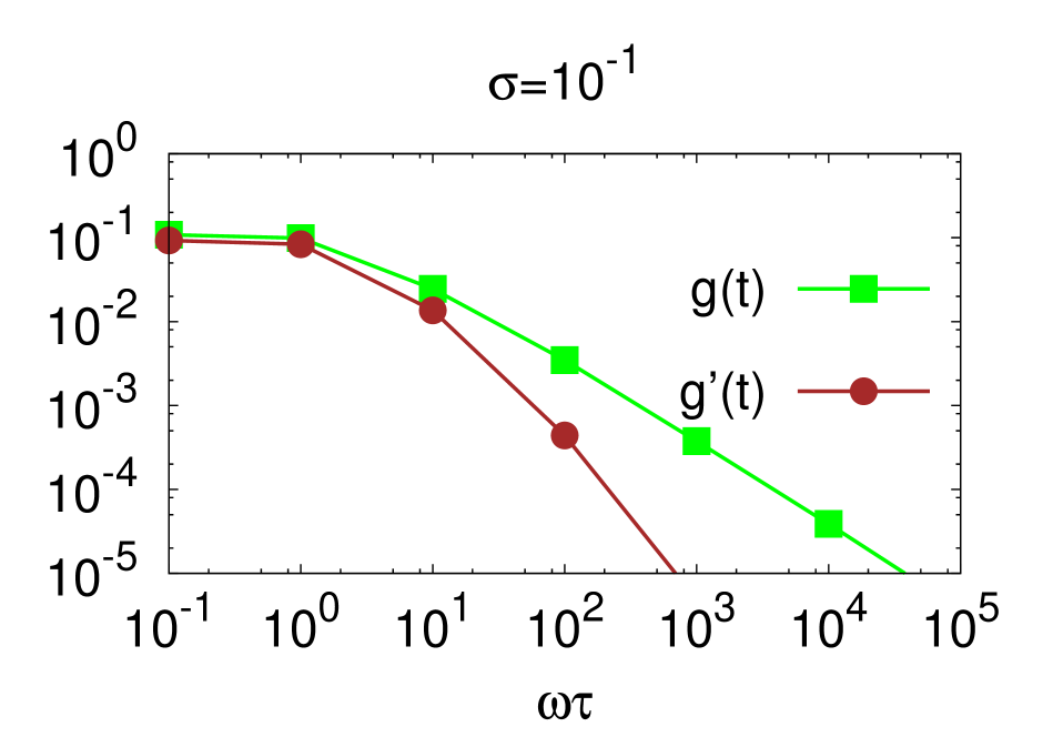
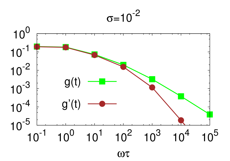
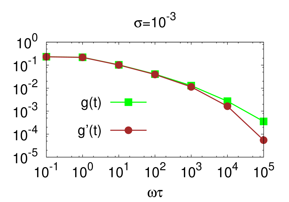
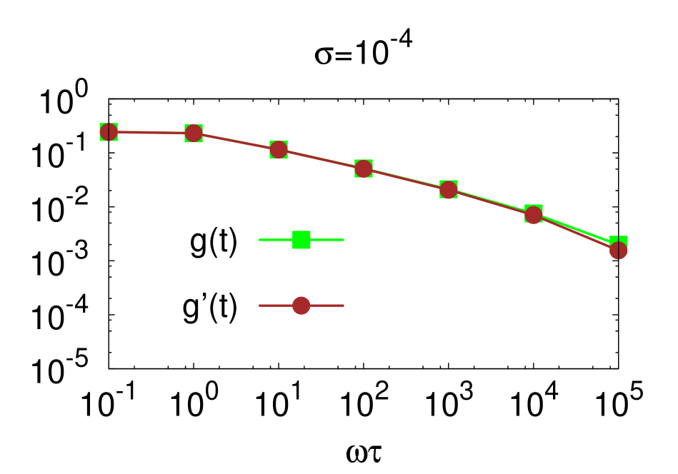
Figure 2: Comparing disorder-averaged non-adiabaticity with non-adiabaticity for disorder-averaged quench parameter. Each panel is for a different standard deviation, $\sigma$, as mentioned above the panel. For a given $\sigma$, the disorder averaged residual energy, $\overline{E}_{r}$, is plotted on the vertical axis, against $\omega\tau$ on the horizontal axis, for the disordered quench, $g(t)$, given by Eq. (17). This is compared with the residual energy (plotted on the same vertical axis) for the disorder-averaged quench, $g^{\prime}(t)$, given by (19). $g^{\prime}(t)$ offers a higher degree of adiabaticity than $g(t)$. The difference in the degree of non-adiabaticities becomes smaller with decrease in $\sigma$. $\overline{E}_{r}$ is in the units of $\hslash\omega$ and $\omega\tau$ is dimensionless.

V Conclusion

Any system driven close to a phase transition unleashes distinct features compared to when its dynamics is considered far away from the same. In particular, a dynamics far away from its critical points of phase transition can be adiabatic for a sufficiently slow quench, whereas this is not possible for quenches near the critical points. Non-adiabaticity for slow quenches in quantum Rabi model has been analyzed in earlier in the literature. The quantum Rabi model, a simplified form of the Dicke model, possesses normal and superradiant phases in the limit when the ratio of atomic transition to cavity field frequencies diverges. We have studied the non-adiabaticity of slow quenches in presence of disorder in the quench of the system governed by the Rabi Hamiltonian. We considered a disordered version of the quench in which system residing in the ground state of an initial Hamiltonian of the normal phase is quenched to the final Hamiltonian corresponding to the critical point. The disorder was assumed to exist either in the total time of the quench or in the quench parameter itself. We numerically simulated the corresponding Schrödinger equations, and obtained that the non-adiabatic effects are unaffected - in terms of the scaling exponents - by the presence of disorder in the total time of the quench. We also independently checked the scaling exponents by using adiabatic perturbation theory and the Kibble-Zurek mechanism. For the case when the disorder is in quench parameter, a monotonic increase in the adiabaticity is reported with the strength of the disorder. We subsequently also considered a quench where the final Hamiltonian is chosen as average over the disordered final Hamiltonians with the disorder being in the quench parameter. We showed that this quench is more adiabatic than the average of the quenches with the disorder in final Hamiltonian quench parameter.

References

- (1) H. Meyer-Ortmanns, Rev. Mod. Phys. 68, 473 (1996).
- (2) L. Amico, R. Fazio, A. Osterloh, and V. Vedral, Rev. Mod. Phys. 80, 517 (2008).
- (3) C. Misbah, O. Pierre-Louis, and Y. Saito, Rev. Mod. Phys. 82, 981 (2010).
- (4) A. Polkovnikov, K. Sengupta, A. Silva, and M. Vengalattore, Rev. Mod. Phys. 83, 863 (2011).
- (5) I. A. Dmitriev, A. D. Mirlin, D. G. Polyakov, and M. A. Zudov Rev. Mod. Phys. 84, 1709 (2012).
- (6) J. Eisert, M. Friesdorf, and C. Gogolin, Nat. Phys. 11, 124 (2015).
- (7) M. Schreiber, S. S. Hodgman, P. Bordia, H. P. Lschen, M. H.Fischer, R. Vosk, E. Altman, U. Schneider, and I. Bloch, Science 349, 842 (2015).
- (8) P. Bordia, H. P. Luschen, S. S. Hodgman, M. Schreiber, I.Bloch, and U. Schneider, Phys. Rev. Lett. 116, 140401 (2016).
- (9) J.-y. Choi, S. Hild, J. Zeiher, P. Schau, A. Rubio-Abadal, T. Yefsah, V. Khemani, D. A. Huse, I. Bloch, and C. Gross, Science 352, 1547 (2016).
- (10) P. Bordia, H. Lüschen, U. Schneider, M. Knap, and I. Bloch, Nat. Phys. 13, 460 (2017).
- (11) P. Bordia, H. Lüschen, S. Scherg, S. Gopalakrishnan, M.Knap, U. Schneider, and I. Bloch, Phys. Rev. X 7, 041047 (2017).
- (12) J. Smith, A. Lee, P. Richerme, B. Neyenhuis, P. W. Hess,P. Hauke, M. Heyl, D. A. Huse, and C. Monroe, Nat. Phys. 12, 907 (2016).
- (13) E. A. Martinez, C. A. Muschik, P. Schindler, D. Nigg, A.Erhard, M. Heyl, P. Hauke, M. Dalmonte, T. Monz, P. Zoller, and R. Blatt, Nature 534, 516 (2016).
- (14) B. Neyenhuis, J. Zhang, P. W. Hess, J. Smith, A. C. Lee, P.Richerme, Z.-X. Gong, A. V. Gorshkov, and C. Monroe, Sci. Adv. 3, e1700672 (2017).
- (15) J. Zhang, G. Pagano, P. W. Hess, A. Kyprianidis, P. Becker,H. Kaplan, A. V. Gorshkov, Z.-X. Gong, and C. Monroe, Nature 551, 601 (2017).
- (16) M. Lewenstein, A. Sanpera, V. Ahufinger, B. Damski, A. Sen(De), and U. Sen, Adv. Phys. 56, 243 (2007).
- (17) I. Buluta and F. Nori, Science 326, 108 (2009).
- (18) M. Lewenstein, A. Sanpera, and V. Ahufinger, Ultracold Atoms in Optical Lattices: Simulating quantum many-body systems (Oxford University Press, 2012).
- (19) I. M. Georgescu, S. Ashhab, and F. Nori, Rev. Mod. Phys. 86, 153 (2014).
- (20) J. I. Cirac and P. Zoller, Nat. Phys. 8, 264 (2012).
- (21) T. Albash and D. A. Lidar, Rev. Mod. Phys. 90, 015002 (2018).
- (22) M. Heyl, A. Polkovnikov, and S. Kehrein, Phys. Rev. Lett. 110, 135704 (2013).
- (23) B. Sciolla and G. Biroli, J. Stat. Mech. (2011) P11003.
- (24) B. Sciolla and G. Biroli, Phys Rev B. 88, 201110(R) (2013).
- (25) A. Gambassi and P. Calabrese, EPL 95, 66007 (2011).
- (26) P. Smacchia, M.l Knap, E. Demler, and A. Silva, Phys. Rev. B 91, 205136 (2015).
- (27) B. Žunkovič, A. Silva, and M. Fabrizio, Phil. Trans. R. Soc. A 374, 20150160 (2016).
- (28) M. Heyl, Rep. Prog. Phys. 81, 054001 (2018).
- (29) J. C. Halimeh, M. Punk, and F. Piazza, Phys. Rev. B 98, 045111 (2018).
- (30) S. Bhattacharjee and A. Dutta, Phys. Rev. B 97, 134306 (2018).
- (31) S. Haldar, S. Roy, T. Chanda, A. Sen(De), and U. Sen, Phys. Rev. B 101, 224304 (2020).
- (32) A. Sehrawat, C. Srivastava, and U. Sen, arXiv:2012.00561.
- (33) M. Born and V. A. Fock, Zeitschrift für Physik A. 51, 165 (1928).
- (34) S. Sachdev, Quantum Phase Transitions (Cambridge University Press, 2011).
- (35) R. H. Dicke, Phys. Rev. 93, 99 (1954).
- (36) R. F. Bishop, N. J. Davidson, R. M. Quick, and D. M. vander Walt, Phys. Rev. A 54, R4657 (1996).
- (37) R. F. Bishop and C. Emary, J. Phys. A 34, 5635 (2001).
- (38) G. Levine and V. N. Muthukumar, Phys. Rev. B 69, 113203 (2004).
- (39) A. P. Hines, C. M. Dawson, R. H. McKenzie, and G. J. Milburn, Phys. Rev. A 70, 022303 (2004).
- (40) L. Bakemeier, A. Alvermann, and H. Fehske, Phys. Rev. A 85, 043821 (2012).
- (41) S. Ashhab and F. Nori, Phys. Rev. A 81, 042311 (2010).
- (42) M.-J. Hwang and M.-S. Choi, Phys. Rev. A 82, 025802 (2010).
- (43) S. Ashhab, Phys. Rev. A 87, 013826 (2013).
- (44) M.-J. Hwang, R. Puebla, and M. B. Plenio, Phys. Rev. Lett. 115, 180404 (2015).
- (45) R. Puebla, M.-J. Hwang, J. Casanova, and M. B. Plenio, Phys. Rev. Lett. 118, 073001 (2017).
- (46) C. De Grandi and A. Polkovnikov, Quantum Quenching, Annealing and Computation, edited by A. K. Chandra, A. Das, and B. K.Chakrabarti (Springer, Heidelberg, 2010).
- (47) T. W. B. Kibble, J. Phys. A 9, 1387 (1976).
- (48) W. H. Zurek, Nature 317, 505 (1985).
- (49) W. H. Zurek, Phys. Rep. 276, 177 (1996).
- (50) P. Laguna and W. H. Zurek, Phys. Rev. Lett. 78, 2519 (1997).
- (51) J. Dziarmaga, Adv. Phys. 59, 1063 (2010).
- (52) A. del Campo and W. H. Zurek, Int. J. Mod. Phys. A 29, 1430018 (2014).
- (53) H. J. Lipkin, N. Meshkov, and A. J. Glick, Nucl. Phys. 62, 188 (1965).
- (54) R. Botet, R. Jullien, and P. Pfeuty, Phys. Rev. Lett. 49, 478 (1982).
- (55) R. Botet and R. Jullien, Phys. Rev. B 28, 3955 (1983).
- (56) A. Polkovnikov, Phys. Rev. B 72, 161201 (2005).
- (57) W. H. Zurek, U. Dorner, and P. Zoller, Phys. Rev. Lett. 95, 105701 (2005).
- (58) J. Dziarmaga, Phys. Rev. Lett. 95, 245701 (2005).
- (59) B. Damski, Phys. Rev. Lett. 95, 035701 (2005).
- (60) B. Damski and W. H. Zurek, Phys. Rev. A 73, 063405 (2006).
- (61) B. Damski and W. H. Zurek, Phys. Rev. Lett. 99, 130402 (2007).
- (62) B. Damski and W. H. Zurek, New J. Phys. 10, 045023 (2008).
- (63) G. Nikoghosyan, R. Nigmatullin, and M. B. Plenio, Phys. Rev. Lett. 116, 080601 (2016).
- (64) D. Braak, Phys. Rev. Lett. 107, 100401 (2011).