Finding nonlinear system equations and complex network structures from data: a sparse optimization approach

Abstract

In applications of nonlinear and complex dynamical systems, a common situation is that the system can be measured but its structure and the detailed rules of dynamical evolution are unknown. The inverse problem is to determine the system equations and structure based solely on measured time series. Recently, methods based on sparse optimization have been developed. For example, the principle of exploiting sparse optimization such as compressive sensing to find the equations of nonlinear dynamical systems from data was articulated in 2011 . This article presents a brief review of the recent progress in this area. The basic idea is to expand the equations governing the dynamical evolution of the system into a power series or a Fourier series of a finite number of terms and then to determine the vector of the expansion coefficients based solely on data through sparse optimization. Examples discussed here include discovering the equations of stationary or nonstationary chaotic systems to enable prediction of dynamical events such as critical transition and system collapse, inferring the full topology of complex networks of dynamical oscillators and social networks hosting evolutionary game dynamics, and identifying partial differential equations for spatiotemporal dynamical systems. Situations where sparse optimization is effective and those in which the method fails are discussed. Comparisons with the traditional method of delay coordinate embedding in nonlinear time series analysis are given and the recent development of model-free, data driven prediction framework based on machine learning is briefly introduced.

I Introduction

In nonlinear dynamics, the traditional solution to the inverse problem, i.e., to analyze time series to probe into the inner “gears” of the system, is based on the paradigm of delay-coordinate embedding Takens (1981); Packard et al. (1980). The research started about four decades ago when Takens Takens (1981) proved that the underlying dynamical system can be faithfully reconstructed from time series with a one-to-one correspondence between the reconstructed and the true but unknown dynamical systems. From the reconstructed system, statistical quantities characterizing the dynamical invariant set of the original system can be assessed Kantz and Schreiber (1997); Hegger et al. (2007). For example, from time series, the fractal dimensions of the underlying chaotic attractor can be estimated Grassberger and Procaccia (1983); Grassberger (1986); Procaccia (1988); Osborne and Provenzale (1989); Lorenz (1991); Ding et al. (1993); Lai et al. (1996); Lai and Lerner (1998), as well as the Lyapunov exponents Wolf et al. (1985); Sano and Sawada (1985); Eckmann and Ruelle (1985); Eckmann et al. (1986); Brown et al. (1991); Sauer et al. (1998); Sauer and Yorke (1999) and some unstable periodic orbits Lathrop and Kostelich (1989); Badii et al. (1994); Pierson and Moss (1995); Pei and Moss (1996); So et al. (1996); Allie and Mees (1997). The continuity and differentiability of the original dynamical system can be tested Pecora et al. (1995); Pecora and Carroll (1996); Pecora et al. (1997); Goodridge et al. (2001); Pecora et al. (2007). Practical issues on determining the basic parameters of delay-coordinate embedding such as the proper time delay Theiler (1986); Liebert and Schuster (1989); Liebert et al. (1991); Buzug and Pfister (1992); Kember and Fowler (1993); Rosenstein et al. (1994); Lai et al. (1996); Lai and Lerner (1998) and the embedding dimension Sauer et al. (1991) were addressed. The Takens’ paradigm was also extended to dynamical systems in the regime of transient chaos Lai and Tél (2011); Jánosi et al. (1994); Jánosi and Tél (1994); Dhamala et al. (2000, 2001); Triandaf et al. (2003) and to systems with a time delay Taylor and Campbell (2007).

There were previous methods on data based identification and forecasting of nonlinear dynamical systems Farmer and Sidorowich (1987); Casdagli (1989); Sugihara et al. (1990); Kurths and Ruzmaikin (1990); Grassberger and Schreiber (1990); Gouesbet (1991); Tsonis and Elsner (1992); Baake et al. (1992); Longtin (1993); Murray (1993); Sauer (1994); Sugihara (1994); Finkenstädt and Kuhbier (1995); Parlitz (1996); Schiff et al. (1996); Szpiro (1997); Hegger et al. (1999, 2000); Sello (2001); Matsumoto et al. (2001); Smith (2002); Judd (2003); Sauer (2004); Tao et al. (2007). One approach is to approximate a nonlinear system by a large collection of linear equations in different regions of the phase space to reconstruct the Jacobian matrices on a proper grid Farmer and Sidorowich (1987); Gouesbet (1991); Sauer (1994) or to fit ordinary differential equations to chaotic data Baake et al. (1992). Approaches based on chaotic synchronization Parlitz (1996) or genetic algorithms Szpiro (1997); Tao et al. (2007) to system-parameter estimation were also investigated. In most studies, short-term predictions can be achieved. For nonstationary systems, the method of over-embedding was introduced Hegger et al. (2000) in which the time-varying parameters were treated as independent dynamical variables so that the essential aspects of determinism of the underlying system can be identified.

Takens’ embedding paradigm, while having evolved into a powerful and effective framework in the past forty years to address the inverse problem in nonlinear dynamical systems, gives only a topological equivalent of the system of interest: it does not give the equations of motion of the original system. As such, the state evolution cannot be predicted, nor critical transitions leading to a possible system collapse upon parameter variations. The inverse problem of determining the system equations from measurements was addressed in 1987 by Crutchfield and McNamara Crutchfield and McNamara (1987), who extended the notion of qualitative information contained in a sequence of observations to deduce the effective equations of motion that give the deterministic portion of the observed behavior. The effective equations, however, may contain additional terms that are not present in the original equations. The idea of using the inverse Frobenius–Perron problem through $L^{\infty}$ to design a dynamical system that is “near” the original system with a desired invariant density was proposed in 2000 by Bollt Bollt (2000). Modeling and nonlinear parameter estimation using the least-squares ($L^{2}$) best approximation (Kronecker product representation) were articulated and analyzed in 2007 by Yao and Bollt Yao and Bollt (2007). In the past decade, the idea of using sparse ($L^{1}$) optimization methods such as compressive sensing Candès et al. (2006a, b); Candes̀ (2006); Donoho (2006); Baraniuk (2007); Candes̀ and Wakin (2008) was articulated Wang et al. (2011a, b, c); Su et al. (2012a, b, 2014a, 2014b); Shen et al. (2014); Su et al. (2016) for discovering the exact equations of motion for certain class of nonlinear and complex dynamical systems EMB . Quite recently, entropic regression for overcoming the problem of outliers in nonlinear system identification was articulated AlMomani et al. (2020).

The principle of sparse optimization for finding the equations of nonlinear dynamical systems from data was first published Wang et al. (2011a) in 2011. The basic idea is that many nonlinear dynamical systems in nature and engineering are governed by smooth functions that can be approximated by series expansions. The inverse problem of determining the system equations then boils down to estimating the coefficients in the series. If the series contain many high-order terms, the total number of coefficients to be estimated will be large. In this case, there is no advantage to use the series expansions and the problem remains as difficult as with the original equations. However, if the system equations are relatively simple in the sense that most coefficients in the series expansions are zero, as in many classical nonlinear dynamical systems, the vector of all the coefficients to be determined will be sparse, rendering applicable and effective sparse optimization methods such as compressive sensing Candès et al. (2006a, b); Donoho (2006); Baraniuk (2007); Candes̀ and Wakin (2008) originally developed in the field of signal processing in engineering and applied mathematics. A virtue common to sparse optimization methods is the low requirement of observation data. In addition to enabling finding equations of nonlinear dynamical systems from data Wang et al. (2011a); Yang et al. (2012), compressive sensing has also been exploited for reconstruction of complex networks with discrete and continuous time nodal dynamics Wang et al. (2011a, c) and evolutionary game dynamics Wang et al. (2011b), for detecting hidden nodes Su et al. (2012b, 2014b), for predicting and controlling network synchronization dynamics Su et al. (2012a), and for reconstructing spreading dynamics based on binary data Shen et al. (2014).

II Principle of discovering system equations from data based on sparse optimization

Compressive sensing solves the following convex optimization problem:

$$\min\|\mathbf{a}\|_{1}\quad\mbox{subject \ to}\quad\mathcal{G}\cdot\mathbf{a}=\mathbf{X},$$ (1)

where $\mathbf{a}$ is a sparse vector to be determined, $\mathcal{G}$ is a known random projection matrix, $\mathbf{X}$ is a measurement vector constructed from the available data, and $\|\mathbf{a}\|_{1}=\sum_{i=1}^{N}|\mathbf{a}_{i}|$ denotes the $L_{1}$ norm of the vector $\mathbf{a}$. Compressive sensing is a paradigm of high-fidelity signal reconstruction using only sparse data Candès et al. (2006a, b); Donoho (2006); Baraniuk (2007); Candes̀ and Wakin (2008), which was originally developed to solve the problem of transmitting massive data sets, such as those collected from a large-scale sensor network. Because of the high dimensionality, direct transmission of such data sets would require a broad bandwidth. However, a common situation with sensor networks is that, most of the time, majority of the sensors are inactive so that the data set collected from the entire network at a time is sparse. For example, say a data set of $N$ points is represented by an $N\times 1$ vector ${\bf a}$, where $N$ is a large integer. Since ${\bf a}$ is sparse, most of its entries are zero and only a small number of $k$ entries are non-zero, where $k\ll N$. One can use a Gaussian random matrix $\mathcal{G}$ of dimension $M\times N$ to obtain an $M\times 1$ vector ${\bf X}$: ${\bf X}=\mathcal{G}\cdot{\bf a}$, where $M\sim k$. Because the dimension of ${\bf X}$ is much smaller than that of the original vector ${\bf a}$, transmitting ${\bf X}$ would require a much smaller bandwidth, provided that ${\bf a}$ can be reconstructed at the receiver end of the communication channel.

The problem of reconstructing the equations of a nonlinear dynamical system from data can be formulated in the compressive sensing framework Wang et al. (2011a); Yang et al. (2012). Consider a general dynamical system described by

$$\frac{d\mathbf{x}}{dt}=\mathbf{F}(\mathbf{x}),$$ (2)

where $\mathbf{x}$ is an $m$-dimensional vector: $\mathbf{x}\equiv\left(x_{1},x_{2},\ldots,x_{m}\right)^{T}$, and $\mathbf{F}(\mathbf{x})$ represents the velocity (vector) field of the system with $m$ components: $\mathbf{F}(\mathbf{x})=\left[F_{1}(\mathbf{x}),F_{2}(\mathbf{x}),\ldots,F_{m}(\mathbf{x})\right]^{T}$. The goal is to determine $\mathbf{F}(\mathbf{x})$ from limited measured time series $\mathbf{x}(t)$. The basic idea Wang et al. (2011a) is to expand the velocity field as a multi-dimensional power series. In particular, the $j$th component of the velocity field can be expanded to order $q$ as

$$F_{j}(\mathbf{x})=\sum^{q}_{l_{1}=0}\sum^{q}_{l_{2}=0}\ldots\sum^{q}_{l_{m}=0}(a_{j})_{l_{1}l_{2}\ldots l_{m}}x_{1}^{l_{1}}x_{2}^{l_{2}}\ldots x_{m}^{l_{m}},$$ (3)

where $(a_{j})_{l_{1}l_{2}\ldots l_{m}}$ ($l_{1},\ldots,l_{m}=1,\ldots,q$) constitute the set of $(1+q)^{m}$ coefficients to be determined from the measurements. If this set of coefficients is dense in the sense that most of them are nontrivial, then resorting to the power series expansion as in Eq. (3) does not lead to any step closer to the solution because the coefficients cannot be determined based on limited measurements. However, if the coefficient set is sparse in that most of its elements are zero, then it would be possible to use compressive sensing to uniquely solve for the nontrivial coefficients. Some well studied nonlinear dynamical systems, such as the classic Lorenz Lorenz (1963) and Rössler Rössler (1976) oscillators, fall into this “sparse” category because their vector fields contain only a few power series terms.

To better understand the mathematical structure of the problem formulation, consider the concrete case of a three-dimensional phase space ($m=3$) and power series expansion up to order three ($n=3$). In this case, the total number of unknown coefficients is $(1+n)^{m}=64$. For convenience, let the dynamical variables be $\mathbf{x}(t)\equiv[x(t),y(t),z(t)]^{T}$. The first component of the vector field can be written as

$$F_{1}(\mathbf{x})=(a_{1})_{000}x^{0}y^{0}z^{0}+(a_{1})_{100}x^{1}y^{0}z^{0}+\ldots+(a_{1})_{333}x^{3}y^{3}z^{3}.$$ (4)

The $N=64$ coefficients to be determined can be organized into a vector, a $N\times 1$-dimensional column vector:

$$\mathbf{a}_{1}\equiv\left(\begin{array}[]{c}(a_{1})_{000}\\ (a_{1})_{100}\\ \ldots\\ (a_{1})_{333}\end{array}\right).$$ (5)

Defining all the combinations of the powers of the dynamical variables in Eq. (4) as a $1\times 64$-dimensional row vector:

$$\mathbf{g}(t)\equiv\left[x^{0}(t)y^{0}(t)z^{0}(t),x^{1}(t)y^{0}(t)z^{0}(t),\ldots,x^{3}(t)y^{3}(t)z^{3}(t)\right],$$ (6)

we can write Eq. (4) as

$$F_{1}[\mathbf{x}(t)]=\mathbf{g}(t)\cdot\mathbf{a}_{1}.$$ (7)

Suppose measurements of the dynamical variables $\mathbf{x}(t)$ are available at $(M+1)$ time instants $t_{0},t_{1},\ldots,t_{M}$, where $M\ll N$. We have

$$\begin{array}[]{c}dx(t_{1})/dt=F_{1}[\mathbf{x}(t_{1})]=\mathbf{g}(t_{1})\cdot\mathbf{a}_{1}\\ dx(t_{2})/dt=F_{1}[\mathbf{x}(t_{2})]=\mathbf{g}(t_{2})\cdot\mathbf{a}_{1}\\ \ldots\\ dx(t_{M})/dt=F_{1}[\mathbf{x}(t_{M})]=\mathbf{g}(t_{M})\cdot\mathbf{a}_{1}.\end{array}$$ (8)

The derivatives can be estimated from the measurements:

$$\frac{dx(t_{i})}{dt}\approx\frac{x(t_{i})-x(t_{i-1})}{\delta t},$$

for $i=1,\ldots,M$. All the $M$ derivatives can be organized into an measurement vector that is $M\times 1$-dimensional:

$$\mathbf{X}=\left(\begin{array}[]{c}dx(t_{1})/dt\\ dx(t_{2})/dt\\ \ldots\\ dx(t_{M})/dt\end{array}\right).$$ (9)

Likewise, the $M$ row vectors $\mathbf{g}(t_{1}),\ldots,\mathbf{g}(t_{M})$, each being $1\times N$ dimensional, can be organized into an $M\times N$ dimensional matrix as

$$\mathcal{G}=\left(\begin{array}[]{c}\mathbf{g}(t_{1})\\ \mathbf{g}(t_{2})\\ \ldots\\ \mathbf{g}(t_{M})\end{array}\right).$$ (10)

Equation (8) can then be written as

$$\mathbf{X}_{M\times 1}=\mathcal{G}_{M\times N}\cdot(\mathbf{a}_{1})_{N\times 1}.$$ (11)

The structure of Eq. (11) is shown in Fig. 1, where $\mathcal{G}$ is the projection matrix. Suppose that the coefficient vector $\mathbf{a}_{1}$ is sparse: it has $k$ nontrivial elements, where $k\ll N$. If the inequality $k\leq M\ll N$ holds, then Eq. (11) is in the standard form of compressive sensing Candès et al. (2006a, b); Donoho (2006); Baraniuk (2007); Candes̀ and Wakin (2008), which is Eq. (1).

Figure 1: Standard form of compressive sensing. The goal is to obtain the optimal solution of the $N$-dimensional coefficient vector $\mathbf{a}$ from the $M$-dimensional measurement vector $\mathbf{X}$ through the projection matrix $\mathcal{G}$ that is $M\times N$ dimensional, where $M\ll N$. The mathematical framework of compressive sensing guarantees an optimal solution insofar as the coefficient vector to be solved is sparse: it has only $k$ nontrivial elements, where $k\leq M$, provided that the projection matrix is random.

Two remarks are in order.

Firstly, the coefficient vector $\mathbf{a}_{1}$ is associated with the velocity field of the first dynamical variable $x$. For any other dynamical variable in Eq. (2), a similar expansion procedure can be carried out. For example, for the second dynamical variable $y$, the coefficient vector $\mathbf{a}_{2}$ of its velocity field can be solved through:

$$\mathbf{Y}_{M\times 1}=\mathcal{G}_{M\times N}\cdot(\mathbf{a}_{2})_{N\times 1},$$ (12)

where $\mathbf{Y}_{M\times 1}$ is the measurement vector constituting the derivatives of $y$ at the measurement points. Note that the projection matrix $\mathcal{G}_{M\times N}$ has the same form in Eqs. (11) and (12).

Secondly, in the mathematical framework of compressive sensing, a requirement is that the projection matrix $\mathcal{G}$ be random with zero correlation among its elements. However, in the power series expansion formulation, the elements of this matrix are distinct combinations of the powers of all the dynamical variables in the system. Since the system is deterministic, nonzero correlations among the matrix elements are inevitable. For chaotic systems, this violation of the randomness condition may not be as severe, since the time evolution of the dynamical variables is effectively random, insofar as the time interval between the adjacent measurement points is reasonably large. Nonetheless, there is no mathematical guarantee that an optimal solution can be obtained for solving the inverse problem in nonlinear dynamical systems through the compressive sensing approach, in spite of previously demonstrated successes Wang et al. (2011a); Yang et al. (2012); Wang et al. (2011c, b); Su et al. (2012b, 2014b, a); Shen et al. (2014).

III Applications

A number of applications of the compressive-sensing based solutions of inverse problems in nonlinear and complex dynamical systems are described.

III.1 Predicting system collapse

When some parameter of a nonlinear dynamical system changes, a bifurcation that leads to the collapse of the system can occur. For example, in a global bifurcation called crisis Grebogi et al. (1983), at the bifurcation point a chaotic attractor collides with its own basin boundary and is destroyed. Let $p$ be the bifurcation parameter and $p_{c}$ be the crisis point. Before the crisis, i.e., $p<p_{c}$, the system functions normally with a sustained chaotic behavior in its time evolution, as shown in Fig. 2(a), where the ordinate represents a typical dynamical variable of the system. Beyond the bifurcation point, the system collapses eventually after exhibiting transient chaos, as shown in Fig. 2(b). The bifurcation is thus a catastrophe that must be prevented. In natural and engineering systems, catastrophic collapse is always a possibility. For example, in electrical power systems, voltage collapse Dhamala and Lai (1999) can occur after the system enters into the state of transient chaos Grebogi et al. (1983); Lai and Tél (2011). In ecology, slow parameter drift caused by environmental deterioration can induce a transition into transient chaos, followed by species extinction McCann and Yodzis (1994); Hastings et al. (2018). For a dynamical system of interest, predicting a catastrophe in advance of its occurrence is of paramount importance. This is a challenging problem when the system equations are unknown and the only available information that one can rely on to make the prediction is time series measured while the system still functions normally.

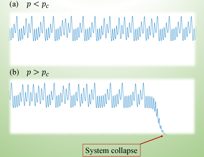
Figure 2: Dynamical behaviors before and after a crisis bifurcation. The bifurcation occurs at the critical parameter value $p_{c}$. (a) Before the crisis ($p<p_{c}$), the system functions normally, as the average values of its dynamical variables maintain at a healthy level, in spite of chaotic fluctuations. (b) After the bifurcation, the system exhibits transient chaos and eventually collapses.

If the underlying equations of the system have a simple mathematical structure, e.g., if its velocity field consists of a few power-series or Fourier-series terms only, then sparse optimization methods such as compressive sensing can be exploited to identify the system equations Wang et al. (2011a, 2016) and consequently to predict transitions. In particular, based on the time series, one first predicts the system equations and then identifies the pertinent parameter of the system that can potentially lead to a collapse. With such information, one can perform a computational bifurcation analysis to locate potential catastrophic events in the parameter space so as to determine the likelihood of system’s drifting into a catastrophic regime. For example, if it is determined that the system currently operates in a parameter region close to the crisis bifurcation, a catastrophe may be imminent as a small parameter change or a random perturbation can push the system into the regime of transient chaos where collapse is inevitable.

The principle of compressive-sensing based prediction of system collapse has been demonstrated with a number of nonlinear dynamical systems Wang et al. (2011a, 2016).

III.2 Predicting future attractors in time-varying dynamical systems

Physical systems are constantly under external influences that can lead to parameter drifting. If the the time scale of the internal dynamics of the system is much faster than that of the external perturbation, the resulting drift in the parameter can be regarded as adiabatic. In this case, in a time window of duration much longer than the internal but shorter than the external time scale, the system can be viewed to be in a kind of “asymptotic state” or an “attractor,” as for the case of a stationary dynamical system with no time-varying parameters. However, in a long time scale, the attractor does depend on time. A problem of significant interest is to forecast the “future” attractor of the system. For example, consider the climate system. It is under random disturbances all the time but adiabatic parameter drifting is also present, such as that induced by the injection of CO₂ into the atmosphere due to human activities. The time scale for any appreciable increase in the CO₂ level (e.g., months or years) is typically much slower than the intrinsic time scales of the system (e.g., days). The climate system can thus be regarded as an adiabatically time-varying, nonlinear dynamical system. To forecast the possible future attractor of the system is key to sustainability, an issue that is critical to many other natural and engineering systems.

It was demonstrated Yang et al. (2012) that predicting the future attractor of an adiabatically time-varying dynamical system can be formulated as a problem solvable by compressive sensing. In particular, let the system be described by

$$d\mathbf{x}/dt=\mathbf{F}[\mathbf{x},\mathbf{p}(t)],$$ (13)

where $\mathbf{x}$ is the set of dynamical variables of the system in the $m$-dimensional phase space and $\mathbf{p}(t)\equiv[p_{1}(t),\ldots,p_{K}(t)]$ denotes $K$ independent, time-varying parameters. The tacit assumption is that both the velocity field $\mathbf{F}$ and the vector parameter function $\mathbf{p}(t)$ are unknown, but only time series $\mathbf{x}(t)$ measured from the system in the time interval $t_{M}-T_{M}\leq t\leq t_{M}$ are available, where $t_{M}$ is the current time. The goal is to determine the precise mathematical forms of $\mathbf{F}$ and $\mathbf{p}(t)$ from the available time series at $t_{M}$ so that the dynamical evolution of the system and the likely attractors for $t>t_{M}$ can be computationally assessed.

As for the case of predicting system collapse discussed in Sec. III.1, the first step is to expand all components of the time-dependent vector field $\mathbf{F}[\mathbf{x},\mathbf{p}(t)]$ into a power series in terms of both dynamical variables $\mathbf{x}$ and time $t$. The $i$th component $\mathbf{F}[\mathbf{x},\mathbf{p}(t)]_{i}$ of the vector field can be written as

$$\sum_{l_{1},\cdots,l_{m}=1}^{n}[(\alpha_{i})_{l_{1},\cdots,l_{m}}x_{1}^{l_{1}}\cdots x_{m}^{l_{m}}\cdot\sum_{w=0}^{v}(\beta_{i})_{w}t^{w}]\equiv\sum_{l_{1},\cdots,l_{m}=1}^{n}\sum_{w=0}^{v}(a_{i})_{l_{1},\cdots,l_{m};w}x_{1}^{l_{1}}\cdots x_{m}^{l_{m}}\cdot t^{w}$$ (14)

where $x_{k}$ ($k=1,\cdots,m$) is the $k$th component of the dynamical variable, $a_{i}$ is the $i$th component of the coefficient vector to be determined, and the time evolution of each term can be approximated by the power series expansion in time, i.e., $\sum_{w=0}^{v}(\beta_{i})_{w}t^{w}$. The power-series expansion can then be cast into the standard form of compressive sensing Eq. (1). If every combined scalar coefficient $(a_{i})_{l_{1},\cdots,l_{m};w}$ associated with the corresponding term in Eq. (14) can be determined from time series for $t\leq t_{M}$, the vector-field component $[{\bf F}({\bf x},{\bf p}(t))]_{i}$ becomes known. Repeating the procedure for all components, the entire vector field for $t>t_{M}$ can be identified.

Note that, the predicted form of $\mathbf{F}$ and $\mathbf{p}(t)$ at time $t_{M}$ would contain errors that in general will increase with time. In addition, for $t>t_{M}$ new perturbations can occur to the system so that the forms of $\mathbf{F}$ and $\mathbf{p}(t)$ may be further changed. It is thus necessary to execute the prediction algorithm frequently using time series available at the time. For example, the system could be monitored at all times so that time series can be collected, and predictions can be carried out at $t_{i}$’s, where $\ldots>t_{i}>\ldots>t_{M+2}>t_{M+1}>t_{M}$. For any $t_{i}$, the prediction algorithm is to be performed based on available time series in a suitable window prior to $t_{i}$.

III.3 Finding complex network structure from data

A class of inverse problems in complex dynamical networks can be stated as follows. Suppose that the connecting structure of a sparse network and the nodal dynamical equations are not known but oscillatory time series can be measured from all nodes in the network. Can the network structure and all the equations of motion of the system be inferred from the measurements? Complex networks in the real world are typically sparse Newman (2010). It turns out that the compressive sensing based approach can be exploited for deciphering the connection structure and the equations of complex oscillator networks Wang et al. (2011c).

An oscillator network can be viewed as a high-dimensional dynamical system that generates oscillatory time series at various nodes, where the local dynamics at a node are described by

$$\dot{\mathbf{x}}_{i}=\mathbf{F}_{i}(\mathbf{x}_{i})+\sum_{j=1,j\neq i}^{n}{\bf C}_{ij}(\mathbf{x}_{j}-\mathbf{x}_{i}),\ \ (i=1,\cdots,n),$$ (15)

where $\mathbf{x}_{i}\in R^{d}$ represents the set of externally accessible dynamical variables of node $i$, $n$ is the number of nodes, and $\mathcal{C}_{ij}$ is the $d\times d$ coupling matrix between the dynamical variables at nodes $i$ and $j$ denoted by

$$\mathcal{C}_{ij}=\left(\begin{array}[]{cccc}c_{ij}^{1,1}&c_{ij}^{1,2}&\cdots&c_{ij}^{1,d}\\ c_{ij}^{2,1}&c_{ij}^{2,2}&\cdots&c_{ij}^{2,d}\\ \cdots&\cdots&\cdots&\cdots\\ c_{ij}^{d,1}&c_{ij}^{d,2}&\cdots&c_{ij}^{d,d}\\ \end{array}\right).$$ (16)

In $\mathcal{C}_{ij}$, the superscripts $kl$ ($k,l=1,2,...,d$) stand for the coupling from the $k$th component of the dynamical variable at node $i$ to the $l$th component of the dynamical variable at node $j$. For any two nodes, the number of possible coupling terms is $d^{2}$. If there is at least one nonzero element in the matrix $\mathcal{C}_{ij}$, nodes $i$ and $j$ are coupled and, as a result, there is a link (or an edge) between them in the network. Generally, more than one element in $\mathcal{C}_{ij}$ can be nonzero. On the contrary, if all the elements of $\mathcal{C}_{ij}$ are zero, there is no coupling between nodes $i$ and $j$. The connecting structure and the interaction strengths among various nodes of the network can be identified if the coupling matrix $\mathcal{C}_{ij}$ can be determined from time-series measurements.

To formulate a solution of the network inverse problem in terms of sparse optimization, the first step is to rewrite Eq. (15) as

$$\dot{\mathbf{x}}_{i}=[\mathbf{F}_{i}(\mathbf{x}_{i})-\sum_{j=1,j\neq i}^{n}\mathcal{C}_{ij}\mathbf{x}_{i}]+\sum_{j=1,j\neq i}^{n}\mathcal{C}_{ij}\mathbf{x}_{j},$$ (17)

where the first term on the right side is exclusively a function of $\mathbf{x}_{i}$ and the second term is a function of variables of other nodes (couplings). The first term can be conveniently denoted as $\mathbf{\Gamma}_{i}(\mathbf{x}_{i})$, which is unknown. The $k$th component of $\mathbf{\Gamma}_{i}(\mathbf{x}_{i})$ can be represented by a power series of order up to $q$:

$$\left[\mathbf{\Gamma}_{i}(\mathbf{x}_{i})\right]_{k}\equiv\left[\mathbf{F}_{i}(\mathbf{x}_{i})-\sum_{j=1,j\neq i}^{n}\mathcal{C}_{ij}\mathbf{x}_{i}\right]_{k}=\sum_{l_{1}=0}^{q}\sum_{l_{2}=0}^{q}\cdots\sum_{l_{d}=0}^{q}[(\mathbf{\alpha}_{i})_{k}]_{l_{1},\cdots,l_{d}}[(\mathbf{x}_{i})_{1}]^{l_{1}}[(\mathbf{x}_{i})_{2}]^{l_{2}}\cdots[(\mathbf{x}_{i})_{d}]^{l_{d}},$$ (18)

where $(\mathbf{x}_{i})_{k}$ ($k=1,\cdots,d$) is the $k$th component of the dynamical variable at node $i$, the total number of products is $(1+q)^{d}$, and $[(\mathbf{\alpha}_{i})_{k}]_{l_{1},\cdots,l_{m}}\in R^{m}$ is the coefficient scalar of each product term, which is to be determined from measurements as well. Note that terms in Eq. (18) are all possible products of different components with different power of exponents. As an example, for $d=2$ (the components are $x$ and $y$) and $q=2$, the power series expansion is

$$\alpha_{0,0}+\alpha_{1,0}x+\alpha_{0,1}y+\alpha_{2,0}x^{2}+\alpha_{0,2}y^{2}+\alpha_{1,1}xy+\alpha_{2,1}x^{2}y+\alpha_{1,2}xy^{2}+\alpha_{2,2}x^{2}y^{2}.$$

The second step is to rewrite Eq. (17) as

$$\dot{\mathbf{x}}_{i}=\mathbf{\Gamma}_{i}(\mathbf{x}_{i})+\mathcal{C}_{i1}\mathbf{x}_{1}+\mathcal{C}_{i2}\mathbf{x}_{2}+\cdots+\mathcal{C}_{in}\mathbf{\bf x}_{n}.$$ (19)

The goal is to estimate the various coupling matrices $\mathcal{C}_{ij}$ $(j=1,\cdots,i-1,i+1,\cdots,n)$ and the coefficients of $\mathbf{\Gamma}_{i}({\bf x}_{i})$ from sparse measurements. The sparsity requirement of the compressive sensing theory stipulates that, to reconstruct the coefficients of Eq. (19) from measurements, most coefficients must be zero. To include as many coupling forms as possible, one can write each term $\mathcal{C}_{ij}\mathbf{x}_{j}$ in Eq. (19) as a power series in the same form of $\mathbf{\Gamma}_{i}(\mathbf{x}_{i})$ but with different coefficients:

$$\dot{\mathbf{x}}_{i}=\mathbf{\Gamma}_{1}(\mathbf{x}_{1})+\mathbf{\Gamma}_{2}(\mathbf{x}_{2})+\cdots+\mathbf{\Gamma}_{n}(\mathbf{x}_{n}).$$ (20)

This setting not only includes many possible coupling forms but also ensures that the sparsity condition is satisfied so that the prediction problem can be formulated in the compressive-sensing framework. For an arbitrary node $i$, information about the node-to-node coupling, or about the network connectivity, is contained completely in $\mathbf{\Gamma}_{j}(j\neq i)$. For example, if in the equation of $i$, a term in $\mathbf{\Gamma}_{j}(j\neq i)$ is not zero, there then exists a coupling between $i$ and $j$ with the strength given by the coefficient of the term. Subtracting the coupling terms $-\sum_{j=1,j\neq i}^{n}\mathcal{C}_{ij}{\bf x}_{i}$ from $\mathbf{\Gamma}_{i}$ in Eq. (18), which is the sum of the coupling coefficients of all $\mathbf{\Gamma}_{j}$ $(j\neq i)$, the local system equations $\mathbf{F}_{i}(\mathbf{x}_{i})$ can be obtained. Therefore, once the coefficients of Eq. (20) have been determined, the nodal dynamical equations and the couplings among the nodes are all known. As explained in Sec. (III.1), the power series expansion coefficients of Eq. (20) can be determined through compressive sensing.

III.4 Finding social network structure from evolutionary game data

In the summer of 2011, a small social network experiment was conducted at Arizona State University, where 22 students from different Schools were invited to test the effectiveness of a sparse-optimization based approach to mapping out the structure of social networks. In particular, the 22 participants constituted a social network, where any individual has a few acquaintances/friends in the group, but many participants had not known each other prior to the experiment. The network is thus sparse. During the experiment, all participants were asked to play an evolutionary game, the prisoner’s dilemma game, with their friends for about 30 runs. That is, each and every agent (node) in the network was asked to play the game but only with his/her direct neighbors. For each run of the play, the strategies used by the opponents of each and every pair of players were recorded, together with the outcome (i.e., the winner and loser). Based on the data from all 30 runs, a compressive sensing based algorithm was executed, yielding a network structure that matches exactly with that of the actual social network. In fact, it was demonstrated that data from about 15 runs were already sufficient to infer the underlying network structure with $100\%$ accuracy Wang et al. (2011b).

The theoretical underpinning of this successful experiment lies in formulating the dynamical process of evolutionary game on a network as a problem of sparse optimization. Specifically, in an evolutionary game, the players use different strategies in order to gain the maximum payoff which, in general, can be divided into two types: cooperation and defection. It was shown Wang et al. (2011b) that, with limited data on each player’s strategy and payoff, a compressive-sensing based framework can be developed to yield precise knowledge of the node-to-node interaction patterns in an efficient manner.

A sketch of the principle underlying the compressive sensing framework is as follows. In an evolutionary game, at any time a player can choose one of the two strategies $S$: cooperation (C) or defection (D), which can be expressed as $\mathbf{S}(C)=(1,0)^{T}$ and $\mathbf{S}(D)=(0,1)^{T}$. The payoffs of two players in a game are determined by their strategies and the payoff matrix of the specific game. For example, for the prisoner’s dilemma game (PDG) Nowak and May (1992) and the snowdrift games (SG) Hauert and Doebeli (2004), the payoff matrices are given, respectively, by

$$\mathcal{P}_{PDG}=\left(\begin{array}[]{cc}1&0\\ b&0\\ \end{array}\right)\ \ \hbox{or}\ \ \mathcal{P}_{SG}=\left(\begin{array}[]{cc}1&1-r\\ 1+r&0\\ \end{array}\right),$$ (25)

where $b$ ($1<b<2$) and $r$ ($0<r<1$) are parameters characterizing the temptation to defect. When a defector encounters a cooperator, the defector gains payoff $b$ in the PDG and payoff $1+r$ in the SG, but the cooperator gains the sucker payoff 0 in the PDG and payoff $1-r$ in the SG. At each time step, all agents play the game with their neighbors and gain payoffs. For agent $i$, the payoff is

$$P_{i}=\sum_{j\in\Gamma_{i}}\mathbf{S}_{i}^{T}\cdot\mathcal{P}\cdot\mathbf{S}_{j},$$ (26)

where $\mathbf{S}_{i}$ and $\mathbf{S}_{j}$ are the strategies of agents $i$ and $j$ at the time and the sum is over the neighboring set $\Gamma_{i}$ of $i$. After obtaining its payoff, an agent updates its strategy according to its own and neighbors’ payoffs, attempting to maximize its payoff at the next round. Possible mathematical prescriptions to describe quantitatively an agent’s decision making process include the best-take-over rule Nowak and May (1992), the Fermi rule Szabó and Tőke (1998), and one based on the payoff-difference-determined updating probability Santos et al. (2008). For example, the Fermi rule is defined, as follows. After player $i$ randomly chooses a neighbor $j$, $i$ adopts $j$’s strategy $\mathbf{S}_{j}$ with the probability Szabó and Tőke (1998):

$$W(\mathbf{S}_{i}\leftarrow\mathbf{S}_{j})=\frac{1}{1+\exp{[(P_{i}-P_{j})/\kappa]}},$$ (27)

where $\kappa$ characterizes the stochastic uncertainties in the evolutionary game dynamics: $\kappa=0$ corresponds to absolute rationality where the probability is zero if $P_{j}<P_{i}$ and one if $P_{i}<P_{j}$, and $\kappa\rightarrow\infty$ indicates completely random decision making. The probability $W$ thus characterizes the bounded rationality of agents in society and the natural selection based on the relative fitness in evolution.

The key to solving the inverse problem of network reconstruction is the relationship between agents’ payoffs and strategies. The interactions among the agents in the network can be characterized by an $n\times n$ adjacency matrix $\mathcal{A}$ with elements $a_{ij}=1$ if agents $i$ and $j$ are connected and $a_{ij}=0$ otherwise. The payoff of agent $x$ can be expressed by

$$P_{x}(t) = a_{x1}\mathbf{S}_{x}^{T}(t)\cdot\mathcal{P}\cdot\mathbf{S}_{1}(t)+\cdots+a_{x,x-1}\mathbf{S}_{x}^{T}(t)\cdot\mathcal{P}\cdot\mathbf{S}_{x-1}(t)+a_{x,x+1}\mathbf{S}_{x}^{T}(t)\cdot\mathcal{P}\cdot\mathbf{S}_{x+1}(t)$$ (28)

$$+ \cdots+\ a_{xn}\mathbf{S}_{x}^{T}(t)\cdot\mathcal{P}\cdot\mathbf{S}_{n}(t),$$

where $a_{xi}$ ($i=1,\cdots,x-1,x+1,\cdots,n$) represents a possible connection between agent $x$ and its neighbor $i$, $a_{xi}\mathbf{S}_{x}^{T}(t)\cdot\mathbf{P}\cdot\mathbf{S}_{i}(t)$ ($i=1,\cdots,x-1,x+1,\cdots,n$) stands for the possible payoff of agent $x$ from playing the game with $i$ (if there is no connection between $x$ and $i$, the payoff is zero because $a_{xi}=0$), and $t=1,\cdots,M$ is the number of rounds that all agents play the game with their neighbors. This relation provides a base to construct the vector $\mathbf{X}_{x}$ and matrix $\mathcal{G}_{x}$ in a proper compressive-sensing framework to obtain the solution of the neighboring vector $\mathbf{A}_{x}$ of agent $x$. In particular, one can define

$$\mathbf{X}_{x} \equiv (P_{x}(t_{1}),P_{x}(t_{2}),\cdots,P_{x}(t_{M}))^{T},$$

$$\mathbf{A}_{x} \equiv (a_{x1},\cdots,a_{x,x-1},a_{x,x+1},\cdots,a_{xn})^{T},$$ (29)

and

$$\mathcal{G}_{x}\equiv\left(\begin{array}[]{cccccc}F_{x1}(t_{1})&\cdots&F_{x,x-1}(t_{1})&F_{x,x+1}(t_{1})&\cdots&F_{xn}(t_{1})\\ F_{x1}(t_{2})&\cdots&F_{x,x-1}(t_{2})&F_{x,x+1}(t_{2})&\cdots&F_{xn}(t_{2})\\ \vdots&\cdots&\vdots&\vdots&\vdots&\vdots\\ F_{x1}(t_{M})&\cdots&F_{x,x-1}(t_{M})&F_{x,x+1}(t_{M})&\cdots&F_{xn}(t_{M})\\ \end{array}\right),$$ (34)

where $F_{xy}(t_{i})=\mathbf{S}_{x}^{T}(t_{i})\cdot\mathcal{P}\cdot\mathbf{S}_{y}(t_{i})$. The relation among the vectors $\mathbf{X}_{x}$, $\mathbf{A}_{x}$, and the matrix $\mathcal{G}_{x}$ is given by exactly the same form as of compressive sensing Eq. (1):

$$\mathbf{X}_{x}=\mathcal{G}_{x}\cdot\mathbf{A}_{x},$$ (35)

where $\mathbf{A}_{x}$ is sparse due to the sparsity of the underlying network, making the compressive-sensing framework applicable. Since $\mathbf{S}_{x}^{T}(t_{i})$ and $\mathbf{S}_{y}(t_{i})$ in $F_{xy}(t_{i})$ come from data and $\mathcal{P}$ is known, the vector $\mathbf{X}_{x}$ can be obtained directly while the matrix $\mathcal{G}_{x}$ can be calculated from the strategy and payoff data. The vector $\mathbf{A}_{x}$ can thus be predicted based solely on the time series game data. Since the self-interaction terms $a_{xx}$ are not included in the vector $\mathbf{A}_{x}$ and the self-column $[F_{xx}(t_{1}),\cdots,F_{xx}(t_{M})]^{T}$ is excluded from the matrix $\mathcal{G}_{x}$, the computation required for compressive sensing can be reduced. In a similar fashion, the neighboring vectors of all other agents can be predicted, yielding the network adjacency matrix

$$\mathcal{A}=(\mathbf{A}_{1},\mathbf{A}_{2},\cdots,\mathbf{A}_{n})$$

and, hence, the connection structure of the underlying social network.

III.5 Sparse optimization based on LASSO and applications in reconstructing complex networks with binary-state dynamics

A generalization of the compressive sensing approach to inverse problems in nonlinear and complex dynamical systems is sparse optimization based on LASSO (Least Absolute Shrinkage and Selection Operator) Han et al. (2015); Li et al. (2017). In statistical and machine learning, LASSO is a regression method that embodies both variable selection and regularization to enhance the prediction accuracy and interpretability of the statistical model it produces Santosa and Symes (1986); Friedman et al. (2001). In particular, LASSO incorporates an $L_{1}$-norm and an error control term to solve the sparse vector $\mathbf{a}$ according to the constraint $\mathcal{G}\cdot\mathbf{a}=\mathbf{X}$ [as in Eq. (1)] from a small amount of data by optimizing

$$\min_{{\bf a}}\Bigl{\{}\dfrac{1}{2M}\|\mathcal{G}\cdot\mathbf{a}-\mathbf{X}\|_{2}^{2}+\lambda\|\mathbf{a}\|_{1}\Bigr{\}}\text{,}$$ (36)

where $\|\mathbf{a}\|_{1}$ is the $L_{1}$ norm of $\mathbf{X}$ assuring the sparsity of the solution, the least squares term $\|\mathcal{G}\cdot\mathbf{a}-\mathbf{X}\|_{2}^{2}$ guarantees the robustness of the solution against noise in the data, and $\lambda$ is a nonnegative regularization parameter that affects the reconstruction performance in terms of the sparsity of the network, which can be determined by a cross-validation method Pedregosa et al. (2011). The advantage of LASSO is similar to that of compressive sensing: the number $M$ of bases (measurements) needed can be much less than the length of $\mathbf{a}$. The LASSO-based sparse optimization method was successfully applied to reconstructing the structures of complex networks Han et al. (2015).

In data based reconstruction of complex networks, a difficult problem is when the nodal dynamical states are discrete and are of the binary type - a situation that arises commonly in nature, technology, and society Barrat et al. (2008). In a networked system hosting binary nodal dynamics, each node can be in one of the two possible states, e.g., being active or inactive in neuronal and gene regulatory networks Kumar et al. (2010), cooperation or defection in networks hosting evolutionary game dynamics Szabó and Fath (2007), being susceptible or infected in epidemic spreading on social and technological networks Pastor-Satorras et al. (2015), and two competing opinions in social communities Shao et al. (2009), etc. The interactions among the nodes are complex and a state change can be triggered either deterministically (e.g., depending on the states of their neighbors) or randomly. Indeed, deterministic and stochastic state changes can account for a variety of emergent phenomena, such as the outbreak of epidemic spreading Granell et al. (2013), cooperation among selfish individuals Santos and Pacheco (2005), oscillations in biological systems Koseska et al. (2013), power blackout Buldyrev et al. (2010), financial crisis Galbiati et al. (2013), and phase transitions in natural systems Balcan and Vespignani (2011). A variety of models have been introduced to gain insights into binary-state dynamics on complex networks Newman (2010), such as the voter models for competition of two opinions Sood and Redner (2005), stochastic propagation models for epidemic spreading Pastor-Satorras and Vespignani (2001), models of rumor diffusion and adoption of new technologies Castellano et al. (2009), cascading failure models Bashan et al. (2013), Ising spin models for ferromagnetic phase transition Krapivsky et al. (2010), and evolutionary games for cooperation and altruism Santos et al. (2008). A general theoretical approach to dealing with networks hosting binary state dynamics was developed Gleeson (2013) based on the pair approximation and the master equations, providing a good understanding of the effect of the network structure on the emergent phenomena.

The problem of reconstructing complex networks with binary-state dynamics is challenging, for three reasons. Firstly, the basic nodal dynamics are governed by the probability to transition between the two states - the switching probability of a node, which depends on the states of its neighbors according to a variety of functions that can be linear, nonlinear, piecewise, or stochastic. If the function that governs the switching probability is unknown, it would be difficult to obtain a solution of the reconstruction problem. Secondly, structural information is often hidden in the binary states of the nodes in an unknown manner and the dimension of the solution space can be high, rendering impractical (computationally prohibitive) brute-force enumeration of all possible network configurations. Thirdly, the presence of measurement noise, missing data, and stochastic effects in the switching probability make the reconstruction task even more challenging, calling for the development of effective methods that are robust against internal and external random effects.

in 2017, a general and robust framework for reconstructing complex networks based solely on the binary states of the nodes without any knowledge about the switching functions was developed Li et al. (2017). The idea was centered about developing a general method to linearize the switching functions from binary data. The data-based linearization method was demonstrated to be applicable to linear, nonlinear, piecewise, or stochastic switching functions. The method allows one to convert the network reconstruction problem into a sparse signal reconstruction problem for local structures associated with each node. In particular, because of the natural sparsity of complex networks, LASSO was used Han et al. (2015); Li et al. (2017) to identify the neighbors of each node in the network from sparse binary data contaminated by noise. The linearization procedure was justified through a number of linear, nonlinear and piecewise binary-state dynamics on a large number of model and real complex networks. For all the models tested, universally high reconstruction accuracy was achieved Li et al. (2017) even for small data amount with noise. Because of its high accuracy, efficiency and robustness against noise and missing data, the reconstruction framework can serve as a general solution to the inverse problem of network reconstruction from binary-state time series, which is key to articulating effective strategies to control complex networks with binary state dynamics.

III.6 Discovering models of spatiotemporal dynamical systems from data

There was an early work on modeling and parameter estimation for coupled oscillators and spatiotemporal dynamical systems based on the Kronecker product presentation Yao and Bollt (2007). In recent years, sparse optimization or learning has been applied to discovering models of spatiotemporal systems described by partial differential equations (PDEs) Rudy et al. (2017); Li et al. (2019); Reinbold and Grigoriev (2019); Gurevich et al. (2019); Reinbold et al. (2020). PDEs for spatiotemporal systems in science and engineering have the general form:

$$\sum^{n}_{i=0}c_{i}\mathbf{f}_{i}(\mathbf{u},\partial_{t}\mathbf{u},\nabla\mathbf{u},\nabla^{2}\mathbf{u},\ldots)=0,$$ (37)

where $c_{i}$’s are constant coefficients and $\mathbf{f}_{i}$’s are vector functions of time and space derivatives of various orders of the vector field $\mathbf{u}$. Usually, symmetry and physical considerations can be used to reduce the number of terms in Eq. (37) and to narrow down the possible functional forms of $\mathbf{f}_{i}$. From the measurement (noisy) spatiotemporal data $\mathbf{u}$, sparse optimization can be used to remove the unnecessary terms and yield a model that contains a small number of terms Rudy et al. (2017); Li et al. (2019); Reinbold and Grigoriev (2019); Gurevich et al. (2019); Reinbold et al. (2020).

In Ref. Reinbold et al. (2020), the following procedure was devised. Consider a system that contains only a single term of the first-order time derivative of the vector field, written as

$$\partial_{t}\mathbf{u}=\sum^{n}_{i=1}c_{i}\mathbf{f}_{i}(\mathbf{u},\nabla\mathbf{u},\nabla^{2}\mathbf{u},\ldots).$$ (38)

To obtain a set of linear equations for sparse optimization, one multiplies a weight vector $\mathbf{w}$ to Eq. (38) and integrates both sides over a number of distinct spatiotemporal domains $\Omega_{l}$ ($l=1,\ldots,L$) to convert Eq. (38) to

$$\mathbf{q}_{0}=\sum^{n}_{i=1}c_{i}\mathbf{q}_{i}=\mathcal{Q}\cdot\mathbf{c},$$ (39)

where $\mathbf{c}\equiv(c_{1},\ldots,c_{n})^{T}$ is the coefficient vector to be determined from data, $\mathbf{q}_{i}$ is an $L$-dimensional column vector with entries given by:

$$q_{i}^{l}=\int_{\Omega_{l}}\mathbf{q}\cdot\mathbf{f}_{i}d\Omega,$$ (40)

and $\mathcal{Q}\equiv(\mathbf{q}_{1},\ldots,\mathbf{q}_{n})$ constitutes the “library” of possible terms $\mathbf{q}_{i}$’s. Note that, the integral in Eq. (40) involves derivatives of the vector field $\mathbf{u}$. If the measurements of $\mathbf{u}$ are noisy, evaluating these derivatives can be problematic. However, performing integration by parts entails transferring the derivatives to the weight vector $\mathbf{w}$, which can be chosen to be smooth.

For $L\geq n$, an iterative sparse regression algorithm can be used to solve Reinbold et al. (2020) the coefficient vector in Eq. (40). Each iteration involves the following form of the solution that minimizes the residual in Eq. (40):

$$\bar{\mathbf{c}}=\mathcal{Q}^{+}\cdot\mathbf{q}_{0},$$ (41)

where $\mathcal{Q}^{+}$ is the pseudoinverse of the matrix $\mathcal{Q}$. Using an empirical thresholding procedure to eliminate dynamically irrelevant terms $\mathbf{q}_{i}$, with the solved sparse coefficient vector $\mathbf{c}$, one can obtain a minimal PDE model from the measurements $\mathbf{u}$. The method was tested Reinbold et al. (2020) with the one-dimensional Kuramoto-Sivashinsky model that has in its solutions spatiotemporal chaos, the two-dimensional Navier-Stokes equation, and the reaction-diffusion equation.

IV Discussion

The principle of exploiting sparse optimization such as compressive sensing to find the equations of nonlinear dynamical systems from data was first articulated Wang et al. (2011a) in 2011. The basic idea is to expand the equations (the velocity field for a continuous time dynamical system or the map function for a discrete time system) of the underlying system into a power series or a Fourier series of a finite number of terms and then to determine the vector of the expansion coefficients based on data through sparse optimization. The sparse optimization principle has been demonstrated to be effective for finding the governing equations of certain types of nonlinear dynamical systems for inferring the detailed connection structures of complex dynamical networks such as oscillator networks and social networks hosting evolutionary game dynamics. In spite of the demonstrated success, limitation and open questions remain.

A key requirement is that the coefficient vector to be determined must be sparse. If the vector field or the map function contains a few power series terms, such as the classical Lorenz Lorenz (1963) or Rössler Rössler (1976) chaotic oscillator, or contains a few Fourier series terms, such as the standard map Chirikov and Izraelev (1973); Chirikov (1979), then sparse optimization can be quite effective and computationally efficient for finding the system equations Wang et al. (2011a). However, if the vector field or the map function contains a large number of terms in its power series or Fourier series expansion so that the coefficient vector to be determined is dense, then the sparse optimization methodology will fail. One such example is the classical Ikeda map Ikeda (1979); Hammel et al. (1985) that describes the propagation of a laser pulse in an optical cavity:

$$\mathbf{F}(x,y)=\left(\begin{array}[]{c}a+b(x\cos{\phi}-y\sin{\phi}\\ b(x\sin{\phi}+y\cos{\phi}\end{array}\right),$$ (42)

with the nonlinear phase variable $\phi$ given by

$$\phi\equiv p-\frac{k}{1+x^{2}+y^{2}},$$ (43)

where $a$, $b$, $k$, and $p$ are parameters. It can be seen that both components of the map function contain an infinite number of power series terms, rendering inapplicable sparse optimization for finding the system equations from data.

In the mathematical formulation of compressive sensing Eq. (1), a requirement is that the projection matrix $\mathcal{G}$ be random, e.g., Gaussian type of random matrices with no correlations among the matrix elements Candès et al. (2006a, b); Donoho (2006); Baraniuk (2007); Candes̀ and Wakin (2008). However, in the power series formulation, e.g., Eq. (11), the elements of the projection matrix are different combinations of the powers of the dynamical variables, which are correlated even for a chaotic system. The demonstrated success in finding the system equations as reviewed in this article thus has no mathematical guarantee. It may also be possible that the “workable” domain of sparse optimization is larger than that guaranteed by rigorous mathematics. To possibly relax the conditions under which sparse optimization is effective remains an open mathematical issue.

Another difficulty with the application of sparse optimization to find system equations from data is the need to collect time series from all dynamical variables of the system. In real world applications, situations are common where only a limited set of the intrinsic dynamical variables of the system are externally accessible. The requirement of observing all dynamical variables thus represents a formidable obstacle to actual application of the sparse optimization methods. This should be contrasted to the traditional delay coordinate embedding paradigm Takens (1981); Packard et al. (1980) where, in principle, measurements from a single dynamical variable are sufficient to reconstruct the phase space of the underlying system. The capability of the embedding paradigm in uncovering the topological and statistical properties of the dynamical invariant set responsible for the observed data notwithstanding, it is unable to yield the system equations.

In the past two or three years, machine learning has emerged as a promising paradigm for predicting the state evolution of nonlinear dynamical systems. In particular, a class of recurrent neural networks Jaeger (2001); Mass et al. (2002); Jaeger and Haas (2004); Manjunath and Jaeger (2013), the so-called reservoir computing machines, have attracted considerable attention since 2017 as a powerful paradigm for model-free, fully data driven prediction of nonlinear and chaotic dynamical systems Haynes et al. (2015); Larger et al. (2017); Pathak et al. (2017); Lu et al. (2017, 2018); Pathak et al. (2018a, b); Carroll (2018); Nakai and Saiki (2018); Roland and Parlitz (2018); Weng et al. (2019); Griffith et al. (2019); Jiang and Lai (2019); Vlachas et al. (2019); Fan et al. (2020); Zhang et al. (2020). A typical reservoir computing machine consists of an input layer, a hidden layer that is usually a complex dynamical network, and an output layer. Time series data from the dynamical system to be predicted are used to train the machine through a series of adjustments to the weights that connect the hidden layer with the output layer. Once the machine has been trained, it can predict the state evolution of the target system for certain duration of time. A well trained reservoir computing machine can thus be viewed as a “replica” of the target system, where temporal synchronization between the two can be maintained Fan et al. (2020). While the machine learning approach does not yield the equations of the system, it can be used to predict the system behavior especially for those that do not meet the sparsity condition.

References

- Takens (1981) F. Takens, “Detecting strange attractors in fluid turbulence,” in Dynamical Systems and Turbulence, Lecture Notes in Mathematics, Vol. 898, edited by D. Rand and L. S. Young (Springer-Verlag, Berlin, 1981) pp. 366–381.
- Packard et al. (1980) N. H. Packard, J. P. Crutchfield, J. D. Farmer, and R. S. Shaw, “Geometry from a time series,” Phys. Rev. Lett. 45, 712 (1980).
- Kantz and Schreiber (1997) H. Kantz and T. Schreiber, Nonlinear Time Series Analysis, 1st ed. (Cambridge University Press, Cambridge, UK, 1997).
- Hegger et al. (2007) R. Hegger, H. Kantz, and R. Schreiber, TISEAN, e-book ed., Hegger:book (http:www.mpipks-dresden.mpg.de tiseanTISEA3.01 index.html, Dresden, 2007).
- Grassberger and Procaccia (1983) P. Grassberger and I. Procaccia, “Measuring the strangeness of strange attractors,” Physica D 9, 189 (1983).
- Grassberger (1986) P. Grassberger, “Do climatic attractors exist?” Nature (London) 323, 609 (1986).
- Procaccia (1988) I. Procaccia, “Complex or just complicated?” Nature (London) 333, 498 (1988).
- Osborne and Provenzale (1989) A. Osborne and A. Provenzale, “Finite correlation dimension for stochastic systems with power-law spectra,” Physica D 35, 357 (1989).
- Lorenz (1991) E. Lorenz, “Dimension of weather and climate attractors,” Nature (London) 353, 241 (1991).
- Ding et al. (1993) M. Ding, C. Grebogi, E. Ott, T. D. Sauer, and J. A. Yorke, “Plateau onset for correlation dimension: when does it occur?” Phys. Rev. Lett. 70, 3872 (1993).
- Lai et al. (1996) Y.-C. Lai, D. Lerner, and R. Hayden, “An upper bound for the proper delay time in chaotic time series analysis,” Phys. Lett. A 218, 30 (1996).
- Lai and Lerner (1998) Y.-C. Lai and D. Lerner, “Effective scaling regime for computing the correlation dimension in chaotic time series analysis,” Physica D 115, 1 (1998).
- Wolf et al. (1985) A. Wolf, J. B. Swift, H. L. Swinney, and J. A. Vastano, “Determining Lyapunov exponents from a time series,” Physica D 16, 285 (1985).
- Sano and Sawada (1985) M. Sano and Y. Sawada, “Measurement of the Lyapunov spectrum from a chaotic time series,” Phys. Rev. Lett. 55, 1082 (1985).
- Eckmann and Ruelle (1985) J. P. Eckmann and D. Ruelle, “Ergodic theory of chaos and strange attractors,” Rev. Mod. Phys. 57, 617 (1985).
- Eckmann et al. (1986) J. P. Eckmann, S. O. Kamphorst, D. Ruelle, and S. Ciliberto, “Liapunov exponents from time series,” Phys. Rev. A 34, 4971 (1986).
- Brown et al. (1991) R. Brown, P. Bryant, and H. D. I. Abarbanel, “Computing the Lyapunov spectrum of a dynamical system from an observed time series,” Phys. Rev. A 43, 2787 (1991).
- Sauer et al. (1998) T. D. Sauer, J. A. Tempkin, and J. A. Yorke, “Spurious Lyapunov exponents in attractor reconstruction,” Phys. Rev. Lett. 81, 4341 (1998).
- Sauer and Yorke (1999) T. D. Sauer and J. A. Yorke, “Reconstructing the Jacobian from data with observational noise,” Phys. Rev. Lett. 83, 1331 (1999).
- Lathrop and Kostelich (1989) D. P. Lathrop and E. J. Kostelich, “Characterization of an experimental strange attractor by periodic orbits,” Phys. Rev. A 40, 4028 (1989).
- Badii et al. (1994) R. Badii, E. Brun, M. Finardi, L. Flepp, R. Holzner, J. Pariso, C. Reyl, and J. Simonet, “Progress in the analysis of experimental chaos through periodic orbits,” Rev. Mod. Phys. 66, 1389 (1994).
- Pierson and Moss (1995) D. Pierson and F. Moss, “Detecting periodic unstable points in noisy chaotic and limit-cycle attractors with applications to biology,” Phys. Rev. Lett. 75, 2124 (1995).
- Pei and Moss (1996) X. Pei and F. Moss, “Characterization of low-dimensional dynamics in the crayfish caudal photoreceptor,” Nature (London) 379, 618 (1996).
- So et al. (1996) P. So, E. Ott, S. J. Schiff, D. T. Kaplan, T. D. Sauer, and C. Grebogi, “Detecting unstable periodic orbits in chaotic experimental data,” Phys. Rev. Lett. 76, 4705 (1996).
- Allie and Mees (1997) S. Allie and A. Mees, “Finding periodic points from short time series,” Phys. Rev. E 56, 346 (1997).
- Pecora et al. (1995) L. M. Pecora, T. L. Carroll, and J. F. Heagy, “Statistics for mathematical properties of maps between time series embeddings,” Phys. Rev. E 52, 3420 (1995).
- Pecora and Carroll (1996) L. M. Pecora and T. L. Carroll, “Discontinuous and nondifferentiable functions and dimension increase induced by filtering chaotic data,” Chaos 6, 432 (1996).
- Pecora et al. (1997) L. M. Pecora, T. L. Carroll, and J. F. Heagy, “Statistics for continuity and differentiability: an application to attractor reconstruction from time series,” Fields Inst. Commun. 11, 49 (1997).
- Goodridge et al. (2001) C. L. Goodridge, L. M. Pecora, T. L. Carroll, and F. J. Rachford, “Detecting functional relationships between simultaneous time series,” Phys. Rev. E 64, 026221 (2001).
- Pecora et al. (2007) L. M. Pecora, L. Moniz, J. Nichols, and T. Carroll, “A unified approach to attractor reconstruction,” Chaos 17, 013110 (2007).
- Theiler (1986) J. Theiler, “Spurious dimension from correlation algorithms applied to limited time series data,” Phys. Rev. A 34, 2427 (1986).
- Liebert and Schuster (1989) W. Liebert and H. G. Schuster, “Proper choice of the time-delay for the analysis of chaotic time-series,” Phys. Lett. A 142, 107 (1989).
- Liebert et al. (1991) W. Liebert, K. Pawelzik, and H. G. Schuster, “Optimal embeddings of chaotic attractors from topological considerations,” Europhys. Lett. 14, 521 (1991).
- Buzug and Pfister (1992) T. Buzug and G. Pfister, “Optimal delay time and embedding dimension for delay-time coordinates by analysis of the glocal static and local dynamic behavior of strange attractors,” Phys. Rev. A 45, 7073 (1992).
- Kember and Fowler (1993) G. Kember and A. C. Fowler, “A correlation-function for choosing time delays in-phase portrait reconstructions,” Phys. Lett. A 179, 72 (1993).
- Rosenstein et al. (1994) M. T. Rosenstein, J. J. Collins, and C. J. D. Luca, “Reconstruction expansion as a geometry-based framework for choosing proper delay times,” Physica D 73, 82 (1994).
- Sauer et al. (1991) T. D. Sauer, J. A. Yorke, and M. Casdagli, “Embedology,” J. Stat. Phys. 65, 579 (1991).
- Lai and Tél (2011) Y.-C. Lai and T. Tél, Transient Chaos - Complex Dynamics on Finite Time Scales, 1st ed. (Springer, New York, 2011).
- Jánosi et al. (1994) J. Jánosi, L. Flepp, and T. Tél, “Exploring transient chaos in an NMR-laser experiment,” Phys. Rev. Lett. 73, 529 (1994).
- Jánosi and Tél (1994) J. Jánosi and T. Tél, “Time-series analysis of transient chaos,” Phys. Rev. E 49, 2756 (1994).
- Dhamala et al. (2000) M. Dhamala, Y.-C. Lai, and E. J. Kostelich, “Detecting unstable periodic orbits from transient chaotic time series,” Phys. Rev. E 61, 6485 (2000).
- Dhamala et al. (2001) M. Dhamala, Y.-C. Lai, and E. J. Kostelich, “Analysis of transient chaotic time series,” Phys. Rev. E 64, 056207 (2001).
- Triandaf et al. (2003) I. Triandaf, E. Bollt, and I. B. Schwartz, “Approximating stable and unstable manifolds in experiments,” Phys. Rev. E 67, 037201 (2003).
- Taylor and Campbell (2007) S. R. Taylor and S. A. Campbell, “Approximating chaotic saddles in delay differential equations,” Phys. Rev. E 75, 046215 (2007).
- Farmer and Sidorowich (1987) J. D. Farmer and J. J. Sidorowich, “Predicting chaotic time series,” Phys. Rev. Lett. 59, 845 (1987).
- Casdagli (1989) M. Casdagli, “Nonlinear prediction of chaotic time series,” Physica D 35, 335 (1989).
- Sugihara et al. (1990) G. Sugihara, B. Grenfell, R. M. May, P. Chesson, H. M. Platt, and M. Williamson, “Distinguishing error from chaos in ecological time series,” Phil. Trans. Roy. Soc. London B 330, 235 (1990).
- Kurths and Ruzmaikin (1990) J. Kurths and A. A. Ruzmaikin, “On forecasting the sunspot numbers,” Solar Phys. 126, 407 (1990).
- Grassberger and Schreiber (1990) P. Grassberger and T. Schreiber, “Nonlinear time sequence analysis,” Int. J. Bif. Chaos 1, 521 (1990).
- Gouesbet (1991) G. Gouesbet, “Reconstruction of standard and inverse vector fields equivalent to a Rössler system,” Phys. Rev. A 44, 6264 (1991).
- Tsonis and Elsner (1992) A. A. Tsonis and J. B. Elsner, “Nonlinear prediction as a way of distinguishing chaos from random fractal sequences,” Nature (London) 358, 217 (1992).
- Baake et al. (1992) E. Baake, M. Baake, H. G. Bock, and K. M. Briggs, “Fitting ordinary differential equations to chaotic data,” Phys. Rev. A 45, 5524 (1992).
- Longtin (1993) A. Longtin, “Nonlinear forecasting of spike trains from sensory neurons,” Int. J. Bif. Chaos 3, 651 (1993).
- Murray (1993) D. B. Murray, “Forecasting a chaotic time series using an improved metric for embedding space,” Physica D 68, 318 (1993).
- Sauer (1994) T. Sauer, “Reconstruction of dynamical systems from interspike intervals,” Phys. Rev. Lett. 72, 3811 (1994).
- Sugihara (1994) G. Sugihara, “Nonlinear forecasting for the classification of natural time series,” Philos. T. Roy. Soc. A. 348, 477 (1994).
- Finkenstädt and Kuhbier (1995) B. Finkenstädt and P. Kuhbier, “Forecasting nonlinear economic time series: A simple test to accompany the nearest neighbor approach,” Empiri. Econ. 20, 243 (1995).
- Parlitz (1996) U. Parlitz, “Estimating model parameters from time series by autosynchronization,” Phys. Rev. Lett. 76, 1232 (1996).
- Schiff et al. (1996) S. J. Schiff, P. So, T. Chang, R. E. Burke, and T. Sauer, “Detecting dynamical interdependence and generalized synchrony through mutual prediction in a neural ensemble,” Phys. Rev. E 54, 6708 (1996).
- Szpiro (1997) G. G. Szpiro, “Forecasting chaotic time series with genetic algorithms,” Phys. Rev. E 55, 2557 (1997).
- Hegger et al. (1999) R. Hegger, H. Kantz, and T. Schreiber, “Practical implementation of nonlinear time series methods: The tisean package,” Chaos 9, 413 (1999).
- Hegger et al. (2000) R. Hegger, H. Kantz, L. Matassini, and T. Schreiber, “Coping with nonstationarity by overembedding,” Phys. Rev. Lett. 84, 4092 (2000).
- Sello (2001) S. Sello, “Solar cycle forecasting: a nonlinear dynamics approach,” Astron. Astrophys. 377, 312 (2001).
- Matsumoto et al. (2001) T. Matsumoto, Y. Nakajima, M. Saito, J. Sugi, and H. Hamagishi, “Reconstructions and predictions of nonlinear dynamical systems: a hierarchical bayesian approach,” IEEE Trans. Signal Proc. 49, 2138 (2001).
- Smith (2002) L. A. Smith, “What might we learn from climate forecasts?” Proc. Nat. Acad. Sci. (USA) 19, 2487 (2002).
- Judd (2003) K. Judd, “Nonlinear state estimation, indistinguishable states, and the extended kalman filter,” Physica D 183, 273 (2003).
- Sauer (2004) T. D. Sauer, “Reconstruction of shared nonlinear dynamics in a network,” Phys. Rev. Lett. 93, 198701 (2004).
- Tao et al. (2007) C. Tao, Y. Zhang, and J. J. Jiang, “Estimating system parameters from chaotic time series with synchronization optimized by a genetic algorithm,” Phys. Rev. E 76, 016209 (2007).
- Crutchfield and McNamara (1987) J. P. Crutchfield and B. McNamara, “Equations of motion from a data series,” Complex Sys. 1, 417 (1987).
- Bollt (2000) E. M. Bollt, “Controlling chaos and the inverse frobenius-perron problem: global stabilization of arbitrary invariant measures,” Int. J. Bif. Chaos 10, 1033 (2000).
- Yao and Bollt (2007) C. Yao and E. M. Bollt, “Modeling and nonlinear parameter estimation with Kronecker product representation for coupled oscillators and spatiotemporal systems,” Physica D 227, 78 (2007).
- Candès et al. (2006a) E. Candès, J. Romberg, and T. Tao, “Robust uncertainty principles: exact signal reconstruction from highly incomplete frequency information,” IEEE Trans. Info. Theory 52, 489 (2006a).
- Candès et al. (2006b) E. Candès, J. Romberg, and T. Tao, “Stable signal recovery from incomplete and inaccurate measurements,” Comm. Pure Appl. Math. 59, 1207 (2006b).
- Candes̀ (2006) E. Candes̀, “Compressive sampling,” in Proceedings of the International Congress of Mathematicians, Vol. 3 (Madrid, Spain, 2006) pp. 1433–1452.
- Donoho (2006) D. Donoho, “Compressed sensing,” IEEE Trans. Info. Theory 52, 1289 (2006).
- Baraniuk (2007) R. G. Baraniuk, “Compressed sensing,” IEEE Signal Process. Mag. 24, 118 (2007).
- Candes̀ and Wakin (2008) E. Candes̀ and M. Wakin, “An introduction to compressive sampling,” IEEE Signal Process. Mag. 25, 21 (2008).
- Wang et al. (2011a) W.-X. Wang, R. Yang, Y.-C. Lai, V. Kovanis, and C. Grebogi, “Predicting catastrophes in nonlinear dynamical systems by compressive sensing,” Phys. Rev. Lett. 106, 154101 (2011a).
- Wang et al. (2011b) W.-X. Wang, Y.-C. Lai, C. Grebogi, and J.-P. Ye, “Network reconstruction based on evolutionary-game data via compressive sensing,” Phys. Rev. X 1, 021021 (2011b).
- Wang et al. (2011c) W.-X. Wang, R. Yang, Y.-C. Lai, V. Kovanis, and M. A. F. Harrison, “Time-series-based prediction of complex oscillator networks via compressive sensing,” EPL (Europhys. Lett.) 94, 48006 (2011c).
- Su et al. (2012a) R.-Q. Su, X. Ni, W.-X. Wang, and Y.-C. Lai, “Forecasting synchronizability of complex networks from data,” Phys. Rev. E 85, 056220 (2012a).
- Su et al. (2012b) R.-Q. Su, W.-X. Wang, and Y.-C. Lai, “Detecting hidden nodes in complex networks from time series,” Phys. Rev. E 85, 065201 (2012b).
- Su et al. (2014a) R.-Q. Su, Y.-C. Lai, and X. Wang, “Identifying chaotic fitzhugh-nagumo neurons using compressive sensing,” Entropy 16, 3889 (2014a).
- Su et al. (2014b) R.-Q. Su, Y.-C. Lai, X. Wang, and Y.-H. Do, “Uncovering hidden nodes in complex networks in the presence of noise,” Sci. Rep. 4, 3944 (2014b).
- Shen et al. (2014) Z. Shen, W.-X. Wang, Y. Fan, Z. Di, and Y.-C. Lai, “Reconstructing propagation networks with natural diversity and identifying hidden sources,” Nat. Commun. 5, 4323 (2014).
- Su et al. (2016) R.-Q. Su, W.-W. Wang, X. Wang, and Y.-C. Lai, “Data based reconstruction of complex geospatial networks, nodal positioning, and detection of hidden node,” R. Soc. Open Sci. 3, 150577 (2016).
- (87) Professor E. M. Bollt from Clarkson University conceived the same idea of exploiting sparse optimization for discovering system equations from data (unpublished, private communication) .
- AlMomani et al. (2020) A. A. R. AlMomani, S. Jie, and E. M. Bollt, “How entropic regression beats the outliers problem in nonlinear system identification,” Chaos 30, 013107 (2020).
- Yang et al. (2012) R. Yang, Y.-C. Lai, and C. Grebogi, “Forecasting the future: is it possible for time-varying nonlinear dynamical systems?” Chaos 22, 033119 (2012).
- Lorenz (1963) E. N. Lorenz, “Deterministic nonperiodic flow,” J. Atmos. Sci. 20, 130 (1963).
- Rössler (1976) O. E. Rössler, “Equation for continuous chaos,” Phys. Lett. A 57, 397 (1976).
- Grebogi et al. (1983) C. Grebogi, E. Ott, and J. A. Yorke, “Crises, sudden changes in chaotic attractors and chaotic transients,” Physica D 7, 181 (1983).
- Dhamala and Lai (1999) M. Dhamala and Y.-C. Lai, “Controlling transient chaos in deterministic flows with applications to electrical power systems and ecology,” Phys. Rev. E 59, 1646 (1999).
- McCann and Yodzis (1994) K. McCann and P. Yodzis, “Nonlinear dynamics and population disappearances,” Ame. Naturalist 144, 873 (1994).
- Hastings et al. (2018) A. Hastings, K. C. Abbott, K. Cuddington, T. Francis, G. Gellner, Y.-C. Lai, A. Morozov, S. Petrivskii, K. Scranton, and M. L. Zeeman, “Transient phenomena in ecology,” Science 361, eaat6412 (2018).
- Wang et al. (2016) W. Wang, Y.-C. Lai, and C. Grebogi, “Data based identification and prediction of nonlinear and complex dynamical systems,” Phys. Rep. 644, 1 (2016).
- Newman (2010) M. E. J. Newman, Networks: An Introduction (Oxford University Press, Oxford, UK, 2010).
- Nowak and May (1992) M. A. Nowak and R. M. May, “Evolutionary games and spatial chaos,” Nature (London) 359, 826 (1992).
- Hauert and Doebeli (2004) C. Hauert and M. Doebeli, “Spatial structure often inhibits the evolution of cooperation in the snowdrift game,” Nature (London) 428, 643 (2004).
- Szabó and Tőke (1998) G. Szabó and C. Tőke, “Evolutionary prisoner’s dilemma game on a square lattice,” Phys. Rev. E 58, 69 (1998).
- Santos et al. (2008) F. C. Santos, M. D. Santos, and J. M. Pacheco, “Social diversity promotes the emergence of cooperation in public goods games,” Nature 454, 213 (2008).
- Han et al. (2015) X. Han, Z. Shen, W.-X. Wang, and Z. Di, “Robust reconstruction of complex networks from sparse data,” Phys. Rev. Lett. 114, 028701 (2015).
- Li et al. (2017) J. Li, Z. Shen, W.-X. Wang, C. Grebogi, and Y.-C. Lai, “Universal data-based method for reconstructing complex networks with binary-state dynamics,” Phys. Rev. E 95, 032303 (2017).
- Santosa and Symes (1986) F. Santosa and W. W. Symes, “Linear inversion of band-limited reflection seismograms,” SIAM J. Sci. Stat. Comp. 7, 1307 (1986).
- Friedman et al. (2001) J. Friedman, T. Hastie, and R. Tibshirani, The Elements of Statistical Learning (Springer, Berlin, 2001).
- Pedregosa et al. (2011) F. Pedregosa, G. Varoquaux, A. Gramfort, V. Michel, B. Thirion, O. Grisel, M. Blondel, P. Prettenhofer, R. Weiss, V. Dubourg, et al., “Scikit-learn: Machine learning in python,” J. Mach. Learn. Res. 12, 2825 (2011).
- Barrat et al. (2008) A. Barrat, M. Barthelemy, and A. Vespignani, Dynamical Processes on Complex Networks (Cambridge University Press, 2008).
- Kumar et al. (2010) A. Kumar, S. Rotter, and A. Aertsen, “Spiking activity propagation in neuronal networks: reconciling different perspectives on neural coding,” Nature Rev. Neuro. 11, 615 (2010).
- Szabó and Fath (2007) G. Szabó and G. Fath, “Evolutionary games on graphs,” Phys. Rep. 446, 97 (2007).
- Pastor-Satorras et al. (2015) R. Pastor-Satorras, C. Castellano, P. Van Mieghem, and A. Vespignani, “Epidemic processes in complex networks,” Rev. Mod. Phys. 87, 925 (2015).
- Shao et al. (2009) J. Shao, S. Havlin, and H. E. Stanley, “Dynamic opinion model and invasion percolation,” Phys. Rev. Lett. 103, 018701 (2009).
- Granell et al. (2013) C. Granell, S. Gómez, and A. Arenas, “Dynamical interplay between awareness and epidemic spreading in multiplex networks,” Phys. Rev. Lett. 111, 128701 (2013).
- Santos and Pacheco (2005) F. C. Santos and J. M. Pacheco, “Scale-free networks provide a unifying framework for the emergence of cooperation,” Phys. Rev. Lett. 95, 098104 (2005).
- Koseska et al. (2013) A. Koseska, E. Volkov, and J. Kurths, “Oscillation quenching mechanisms: Amplitude vs. oscillation death,” Phys. Rep. 531, 173 (2013).
- Buldyrev et al. (2010) S. V. Buldyrev, R. Parshani, G. Paul, H. E. Stanley, and S. Havlin, “Catastrophic cascade of failures in interdependent networks,” Nature 464, 1025 (2010).
- Galbiati et al. (2013) M. Galbiati, D. Delpini, and S. Battiston, “The power to control,” Nat. Phys. 9, 126 (2013).
- Balcan and Vespignani (2011) D. Balcan and A. Vespignani, “Phase transitions in contagion processes mediated by recurrent mobility patterns,” Nat. Phys. 7, 581 (2011).
- Sood and Redner (2005) V. Sood and S. Redner, “Voter model on heterogeneous graphs,” Phys. Rev. Lett. 94, 178701 (2005).
- Pastor-Satorras and Vespignani (2001) R. Pastor-Satorras and A. Vespignani, “Epidemic spreading in scale-free networks,” Phys. Rev. Lett. 86, 3200 (2001).
- Castellano et al. (2009) C. Castellano, S. Fortunato, and V. Loreto, “Statistical physics of social dynamics,” Rev. Mod. Phys. 81, 591 (2009).
- Bashan et al. (2013) A. Bashan, Y. Berezin, S. V. Buldyrev, and S. Havlin, “The extreme vulnerability of interdependent spatially embedded networks,” Nat. Phys. 9, 667 (2013).
- Krapivsky et al. (2010) P. L. Krapivsky, S. Redner, and E. Ben-Naim, A Kinetic View of Statistical Physics (Cambridge University Press, 2010).
- Gleeson (2013) J. P. Gleeson, “Binary-state dynamics on complex networks: pair approximation and beyond,” Phys. Rev. X 3, 021004 (2013).
- Rudy et al. (2017) S. Rudy, S. L. Brunton, J. L. Proctor, and J. N. Kutz, “Data-driven discovery of partial differential equations,” Sci. Adv. 3, e1602614 (2017).
- Li et al. (2019) X. Li, L. Li, Z. Yue, X. Tang, H. U. Voss, J. Kurths, and Y. Y., “Sparse learning of partial differential equations with structured dictionary matrix,” Chaos 29, 043130 (2019).
- Reinbold and Grigoriev (2019) P. A. K. Reinbold and R. O. Grigoriev, “Data-driven discovery of partial differential equation models with latent variables,” Phys. Rev. E 100, 022219 (2019).
- Gurevich et al. (2019) D. R. Gurevich, P. A. K. Reinbold, and R. O. Grigoriev, “Robust and optimal sparse regression for nonlinear pde models,” Chaos 29, 103113 (2019).
- Reinbold et al. (2020) P. A. K. Reinbold, D. R. Gurevich, and R. O. Grigoriev, “Using noisy or incomplete data to discover models of spatiotemporal dynamics,” Phys. Rev. E 101, 010203 (2020).
- Chirikov and Izraelev (1973) B. V. Chirikov and F. M. Izraelev, “Some numerical experiments with a nonlinear mapping: Stochastic component,” Colloques. Int. du CNRS 229, 409 (1973).
- Chirikov (1979) B. V. Chirikov, “A universal instability of many-dimensional oscillator systems,” Phys. Rep. 52, 263 (1979).
- Ikeda (1979) K. Ikeda, “Multiple-valued stationary state and its instability of the transmitted light by a ring cavity system,” Opt. Commun. 30, 257 (1979).
- Hammel et al. (1985) S. M. Hammel, C. K. R. T. Jones, and J. V. Moloney, “Global dynamical behavior of the optical field in a ring cavity,” J. Opt. Soc. Am. B 2, 552 (1985).
- Jaeger (2001) H. Jaeger, “The “echo state” approach to analysing and training recurrent neural networks-with an erratum note,” Bonn, Germany: German National Research Center for Information Technology GMD Technical Report 148, 13 (2001).
- Mass et al. (2002) W. Mass, T. Nachtschlaeger, and H. Markram, “Real-time computing without stable states: A new framework for neural computation based on perturbations,” Neur. Comp. 14, 2531 (2002).
- Jaeger and Haas (2004) H. Jaeger and H. Haas, “Harnessing nonlinearity: Predicting chaotic systems and saving energy in wireless communication,” Science 304, 78 (2004).
- Manjunath and Jaeger (2013) G. Manjunath and H. Jaeger, “Echo state property linked to an input: Exploring a fundamental characteristic of recurrent neural networks,” Neur. Comp. 25, 671 (2013).
- Haynes et al. (2015) N. D. Haynes, M. C. Soriano, D. P. Rosin, I. Fischer, and D. J. Gauthier, “Reservoir computing with a single time-delay autonomous Boolean node,” Phys. Rev. E 91, 020801 (2015).
- Larger et al. (2017) L. Larger, A. Baylón-Fuentes, R. Martinenghi, V. S. Udaltsov, Y. K. Chembo, and M. Jacquot, “High-speed photonic reservoir computing using a time-delay-based architecture: Million words per second classification,” Phys. Rev. X 7, 011015 (2017).
- Pathak et al. (2017) J. Pathak, Z. Lu, B. Hunt, M. Girvan, and E. Ott, “Using machine learning to replicate chaotic attractors and calculate Lyapunov exponents from data,” Chaos 27, 121102 (2017).
- Lu et al. (2017) Z. Lu, J. Pathak, B. Hunt, M. Girvan, R. Brockett, and E. Ott, “Reservoir observers: Model-free inference of unmeasured variables in chaotic systems,” Chaos 27, 041102 (2017).
- Lu et al. (2018) Z. Lu, B. R. Hunt, and E. Ott, “Attractor reconstruction by machine learning,” Chaos 28, 061104 (2018).
- Pathak et al. (2018a) J. Pathak, A. Wilner, R. Fussell, S. Chandra, B. Hunt, M. Girvan, Z. Lu, and E. Ott, “Hybrid forecasting of chaotic processes: Using machine learning in conjunction with a knowledge-based model,” Chaos 28, 041101 (2018a).
- Pathak et al. (2018b) J. Pathak, B. Hunt, M. Girvan, Z. Lu, and E. Ott, “Model-free prediction of large spatiotemporally chaotic systems from data: A reservoir computing approach,” Phys. Rev. Lett. 120, 024102 (2018b).
- Carroll (2018) T. L. Carroll, “Using reservoir computers to distinguish chaotic signals,” Phys. Rev. E 98, 052209 (2018).
- Nakai and Saiki (2018) K. Nakai and Y. Saiki, “Machine-learning inference of fluid variables from data using reservoir computing,” Phys. Rev. E 98, 023111 (2018).
- Roland and Parlitz (2018) Z. S. Roland and U. Parlitz, “Observing spatio-temporal dynamics of excitable media using reservoir computing,” Chaos 28, 043118 (2018).
- Weng et al. (2019) T. Weng, H. Yang, C. Gu, J. Zhang, and M. Small, “Synchronization of chaotic systems and their machine-learning models,” Phys. Rev. E 99, 042203 (2019).
- Griffith et al. (2019) A. Griffith, A. Pomerance, and D. J. Gauthier, “Forecasting chaotic systems with very low connectivity reservoir computers,” Chaos 29, 123108 (2019).
- Jiang and Lai (2019) J. Jiang and Y.-C. Lai, “Irrelevance of linear controllability to nonlinear dynamical networks,” Nat. Commun. 10, 3961 (2019).
- Vlachas et al. (2019) P. R. Vlachas, J. Pathak, B. R. Hunt, T. P. Sapsis, M. Girvan, E. Ott, and P. Koumoutsakos, “Forecasting of spatio-temporal chaotic dynamics with recurrent neural networks: A comparative study of reservoir computing and backpropagation algorithms,” arXiv preprint arXiv:1910.05266 (2019).
- Fan et al. (2020) H. Fan, J. Jiang, C. Zhang, X. Wang, and Y.-C. Lai, “Long-term prediction of chaotic systems with machine learning,” Phys. Rev. Research 2, 012080 (2020).
- Zhang et al. (2020) C. Zhang, J. Jiang, S.-X. Qu, and Y.-C. Lai, “Predicting phase and sensing phase coherence in chaotic systems with machine learning,” Chaos 30, 083114 (2020).