Quantifying vegetation biophysical variables from imaging spectroscopy data: a review on retrieval methods

Abstract

An unprecedented spectroscopic data stream will soon become available with forthcoming Earth-observing satellite missions equipped with imaging spectroradiometers. This data stream will open up a vast array of opportunities to quantify a diversity of biochemical and structural vegetation properties. The processing requirements for such large data streams require reliable retrieval techniques enabling the spatio-temporally explicit quantification of biophysical variables. With the aim of preparing for this new era of Earth observation, this review summarizes the state-of-the-art retrieval methods that have been applied in experimental imaging spectroscopy studies inferring all kinds of vegetation biophysical variables. Identified retrieval methods are categorized into: (1) parametric regression, including vegetation indices, shape indices and spectral transformations; (2) non-parametric regression, including linear and non-linear machine learning regression algorithms; (3) physically-based, including inversion of radiative transfer models (RTMs) using numerical optimization and look-up table approaches; and (4) hybrid regression methods, which combine RTM simulations with machine learning regression methods. For each of these categories, an overview of widely applied methods with application to mapping vegetation properties is given. In view of processing imaging spectroscopy data, a critical aspect involves the challenge of dealing with spectral multicollinearity. The ability to provide robust estimates, retrieval uncertainties and acceptable retrieval processing speed are other important aspects in view of operational processing. Recommendations towards new-generation spectroscopy-based processing chains for operational production of biophysical variables are given.

Keywords: Imaging spectroscopy, Retrieval, Vegetation products, Parametric and non-parametric regression, Machine learning, Radiative transfer models, Inversion, Uncertainties

1 Introduction

Quantitative vegetation variable extraction is fundamental to assess the dynamic response of vegetation to changing environmental conditions. Earth observation sensors in the optical domain enable the spatiotemporally-explicit retrieval of plant biophysical variables. This data stream has never been so rich as is foreseen with the new generation imaging spectrometer missions. The forthcoming EnMAP (Guanter et al, 2015), HyspIRI (Lee et al, 2015), PRISMA (Labate et al, 2009) and FLEX (Drusch et al, 2017) satellite missions will produce large spectroscopic data streams for land monitoring, which will soon become available to a diverse user community. This upcoming vast data stream will not only be standardized (e.g. atmospherically-corrected), but will also require reliable and efficient retrieval processing techniques that are accurate, robust and fast.

Since the advent of optical remote sensing science, a variety of retrieval methods for vegetation attribute extraction emerged. Most of these methods have been applied to the data of traditional multispectral sensors (Verrelst et al, 2015), but increasingly they are also applied within imaging spectroscopy studies. This review provides a summary of recently developed methodologies to infer per-pixel biophysical variables from imaging spectroscopy data, covering the visible, near-infrared (NIR) and shortwave infrared spectral regions. Essentially, quantification of surface biophysical variables from spectral data always relies on a model, enabling the interpretation of spectral observations and their translation into a surface biophysical variable. Biophysical variable retrievals, as traditionally described in terrestrial remote sensing literature, are grouped into two categories: (1) the statistical (or variable-driven) category; and (2) the physical (or radiometric data-driven) category (Baret and Buis, 2008). Over the last decade, however, both methodological categories expanded into subcategories and combinations thereof. Exemplary is the increasing number of elements of both categories which have been integrated into hybrid approaches. This methodological expansion, therefore, demands for a more systematic categorization. From an optical remote sensing point of view, and in line with an earlier, more general review paper (Verrelst et al, 2015), retrieval methods can be classified in the following four methodological categories:

1. Parametric regression methods: Parametric methods assume an explicit relationship between spectral observations and a specific biophysical variable. Thus, explicit parameterized expressions are built usually based on some physical knowledge of absorption and scattering properties and statistical relationship between the variable and the spectral response. Typically a band arithmetic formulation is defined (e.g., a spectral index) and then linked to the variable of interest based on a fitting function.

2. Non-parametric regression methods: Non-parametric methods directly define regression functions according to information from the given spectral data and associated variable, i.e., they are data-driven methods. Hence, in contrast to parametric regression methods, a non-explicit choice is to be made on spectral band relationships, transformation(s) or fitting function. Non-parametric methods can further be split into linear or nonlinear regression methods.

3. Physically-based model inversion methods: Physically-based algorithms are applications of physical laws establishing photon interaction cause-effect relationships. Model variables are inferred based on specific knowledge, typically obtained with radiative transfer functions.

4. Hybrid regression methods: A hybrid-method combines elements of non-parametric statistics and physically-based methods. Hybrid models rely on the generic properties of physically-based methods combined with the flexibility and computational efficiency of non-parametric nonlinear regression methods.

These categories provide a theoretical framework to organize the myriad of retrieval methods, as well to overview the diversity of published imaging spectroscopy applications based on these methods. However, a few remarks must be considered. One should be aware that the boundaries of these categories are not always clearly defined; for instance, spectral indices are also often used as input into non-parametric methods. Another important aspect is that the majority of the here reviewed methods is not exclusively designed for retrieval of biophysical variables. This especially holds for the statistical methods, whereby a regression model is used to link spectral data with a biophysical variable. In optical remote sensing science these methods are commonly applied to map any feasible continuous variable, as well in the domains of snow, water or soil properties (see Matthews (2011), Mulder et al (2011) and Dietz et al (2012) for reviews). Nevertheless, to keep this review comprehensive, it is limited to retrieval methods with applications in the domain of vegetation properties mapping. On the other hand, even within these boundaries each of the above methodological categories continue to be expanded with all kinds of spectroscopic data processing applications (e.g. Gewali et al, 2018). The drivers behind this methodological expansion can be found in the: (1) interminable increase of computational power, (2) the increasing availability and democratizing of spectroscopic data, and (3) the steady progress in imaging spectroscopy sensor technology, which produces each time more sensitive sensors. This progress in imaging spectroscopy technology enables to infer each time more subtle and highly dynamic vegetation properties from spectral data. For instance, the forthcoming FLEX mission aims to deliver a portfolio of dynamic plant stress and productivity variables based on, among others, the exploitation of sun-induced chlorophyll fluorescence emitted by terrestrial vegetation (Drusch et al, 2017). Hence, this underlines the fact that the list of biophysical variables that can be extracted from imaging spectroscopy is not closed, but instead continues to grow with ongoing progress in spectrometer technology. Consequently, biophysical variables are in this review paper defined as any vegetation property that can be quantified, i.e. any pigments, chemical constituents, structural variables, but also variables related to plant photosynthesis, productivity or diseases. Altogether, the drivers behind methodological expansion are not mutually exclusive, but they strengthen each other, which leads to a rapid progress in the development of advanced retrieval methods that goes hand in hand with improved capabilities to quantify a broad diversity of biophysical variables. As will be demonstrated throughout this review, these trends are resulting in an unprecedented richness of imaging spectroscopy mapping applications.

Regardless of the used methodology or the targeted application, the principal characteristic of spectroscopic data lies in their dense information content embedded in a few hundred spectrally narrow bands. Although such spectrally dense data source proved to be beneficial for the majority of targeted mapping applications, a key challenge for many retrieval methods is how to deal with spectral multicollinearity, i.e. band redundancy. Special attention, therefore, will be devoted to address common spectroscopic data processing challenges, and solutions will be given how to overcome them. Finally, while imaging spectrometers are so far mostly applied in an experimental context, the developments towards operational systems have manifestly taken off – and undoubtedly will lead to new directions and possibilities of Earth observation. In view of getting prepared for these upcoming global spectroscopic data streams, we will close this review with recommendations about the possibilities of integrating promising retrieval approaches into operational schemes.

2 Parametric regression methods

Parametric regression methods have long been the most popular method to quantify biophysical variables in optical remote sensing; and the field of imaging spectroscopy is no exception to that. This simplest way of developing a regression model explicitly determines parameterized expressions relating a limited number of spectral bands with a biophysical variable of interest. The empirical models rely on a selection of bands with high sensitivity towards the variable of interest, typically in combination with subtle spectral features to reduce undesired effects; related to variations of, for instance, other leaf or canopy properties, background soil reflectance, solar illumination and sensor viewing geometry and atmospheric composition (e.g. Verrelst et al, 2008, 2010). In the following overview we present common parametric regression methods, which are based on (1) vegetation indices, (2) shape indices, and (3) spectral transformations.

Figure 1: Principles of parametric regression. Left: RGB subset of a hyperspectral HyMap image (125 bands) over Barrax agricultural site (Spain). Right: illustrative map of a vegetation property (LAI, m²/m²) as obtained by a 2-band normalized difference index and linear regression. The model was validated with a R² of 0.89 (RMSE: 0.63; NRMSE 10.1%). It took 0.2 seconds to produce the map using ARTMO’s SI toolbox (Rivera et al, 2014). No uncertainty estimates are provided.

2.1 Discrete spectral band approaches: vegetation indices

Parametric regression models based on vegetation indices (VIs) are by far the oldest and largest group of variable estimation approaches. VIs are defined to enhance spectral features sensitive to a vegetation property, while reducing disturbances by combining some spectral bands into a VI (Glenn et al, 2008; Clevers, 2014). The main advantage of VIs is their intrinsic simplicity. VI-based methods found their origin in the first applications of broadband sensor satellites. During the pioneering years of optical remote sensing only a small set of spectral bands were available and computational power was limited. It led to a long tradition of the development of simple two-bands, or at most three to four band indices that continues until today (e.g. Kira et al, 2016). New possibilities have opened with the advent of imaging spectrometers. Optimized narrowband information extraction algorithms were developed based on adaptations of established index formulations, such as simple ratio, normalized difference (see reviews Glenn et al (2008); Clevers (2014); Xue and Su (2017)). On the other hand, the possibilities to develop spectral indices based on a few band combinations grew exponentially, and it demanded for more systematic band evaluation methods.

A popular solution involves correlating all possible band combinations according to established index formulations. For two-band index formulations, such as simple ratio or normalized difference, this approach leads to 2D correlation matrices, which enables to visually identify optimal band combinations (e.g. Thenkabail et al, 2000; le Maire et al, 2004, 2008; Atzberger et al, 2010; Mariotto et al, 2013; Rivera et al, 2014). Subsequently, given all possible combinations permits to select a ’best performing index’. Nevertheless, while being mathematically simple, this method is not only tedious – especially when evaluating all possible combinations of more than two bands – but also keeps on being restricted to formulations that make use of a few bands only, with at most using three or four bands. Thus, although the approach is systematic, it continues to underexploit the comprehensive information content hidden in the contiguous spectral data. Moreover, when applying this technique in mapping applications making use of imaging spectroscopy, identical best performing spectral band combinations for the same biophysical variable have rarely been reported. This suggests that optimized narrowband VIs are strongly case specific and seem to lack generic capacity (Gonsamo, 2011; Heiskanen et al, 2013; Mariotto et al, 2013).

More fundamentally, it remains dubious whether relying on transformed data originating from a few discrete bands fully captures the complexity of real world observation conditions as has been observed by a spectroradiometer. Reducing full-spectrum datasets into simple indices formulations intrinsically leads to remaining spectral information left unexploited. Accordingly, the following two aspects should be considered to ensure optimized use of VIs in a spectroscopic context: (1) Band selection. Spectral indices are mathematical functions based on discrete bands, or at best a subset of full spectral information. Thus, the question arises: how do we assess with high enough accuracy whether the most sensitive spectral bands – with respect to biophysical variable retrieval – have been selected? (2) Formulation. Enhancing spectral information according to a mathematical transformation should lead to an optimal sensitivity of the spectral signal with respect to the variable of interest. While established formulations such as the simple ratio or normalized difference are commonly used, here the question arises again: how can we be sure whether these linear formulations are the most powerful ones with respect to biophysical variable retrieval? These two questions are almost impossible to resolve considering the unlimited possibilities of band selections together with designing index formulations. Consequently, given their inherent constraints, it can be be concluded that VI-based regression models exploit spectroscopic data suboptimally.

2.2 Parametric approaches based on spectral shapes and spectral transformations

Because none of the above few-band indices methods take full advantage of spectroscopic datasets, alternative methods were pursued with the advent of hyperspectral spectroradiometers that allow to exploit specific absorption regions of the reflectance spectrum. It led to the development of so-called shape indices and spectral transformation methods. Shape indices, listed below, extract shape-related information from contiguous spectral signatures for a specific spectral region that is then correlated with a biophysical variable. These types of parametric methods are therefore exclusively applicable to spectroscopic data. The following categories can be identified:

• Red-edge position (REP) calculations. Mathematically, the REP inflection point is the position of a wavelength defined as the maximum of the first derivative reflectance between the red and NIR regions, i.e., between 670 and 780 nm (Kanke et al, 2016). The red-edge position is known to be sensitive to multiple biophysical variable variations, both chlorophyll pigments (Delegido et al, 2011) as well as structural variables, for instance the leaf area index (LAI) (Delegido et al, 2013). Therefore, REP-related methods are typically used to derive canopy chlorophyll content, being the product of LAI and leaf chlorophyll content (Clevers and Kooistra, 2012; Li et al, 2017). Many mathematical approaches have been proposed to exploit this region as a sensitive indicator, including: (1) high-order curve fitting (Broge and Leblanc, 2001; Clevers et al, 2004); (2) inverted Gaussian models (Miller et al, 1990; Cho and Skidmore, 2006; Cho et al, 2008); (3) linear interpolation and extrapolation methods (Cho et al, 2008; Tian et al, 2011); (4) Lagrangian interpolation (Dawson et al, 1998; Pu et al, 2003); (5) rational function application (Baranoski and Rokne, 2005); and more recently, (6) a wavelet-based technique (Li et al, 2017).

• Derivative-based indices. Although several of the above-described methods make use of derivatives, e.g. linear extrapolation (Cho and Skidmore, 2006) and Lagrangian technique (Dawson et al, 1998), the calculation of a derivative does not have to be restricted to the red edge. The derivative of any spectral region can be calculated and transformed into an index (Penuelas et al, 1994; Elvidge and Chen, 1995; Sims and Gamon, 2002; Zarco-Tejada et al, 2002). A systematic comparison of first derivative-based indices and conventional indices was performed by le Maire et al (2004) using the leaf optical model PROSPECT. Interestingly, the authors concluded that derivative-based indices are not necessarily better than conventional and properly elaborated indices.

• Integration-based indices. Alternatively, some authors proposed to calculate finite integrals of specific spectral regions, typically covering a part of the visible and the red-edge region for LAI or chlorophyll content estimations, into a (normalized) index (Broge and Leblanc, 2001; Oppelt and Mauser, 2004; Mutanga et al, 2005; Malenovský et al, 2006, 2015; Delegido et al, 2010). Likewise, in a recent study of Pasqualotto et al (2018) this method exploited the water absorption spectral regions to quantify canopy water content. In these studies, integration-based indices were demonstrated to perform superior to classical vegetation indices, as they exploit more optimally absorption regions embedded in spectroscopic data than indices relying on a reflectance intensity of few individual bands (Kováč et al, 2013). It can be expected that with the upcoming free availability of imaging spectroscopy data more of this kind of methods that explicitly exploit absorption features related to foliar constituents and pigments will emerge.

• Continuum removal. Whereas the above techniques focus on one or more specific spectral regions, continuum removal is a spectral transformation that can be applied over the full spectrum. This technique normalizes reflectance spectra, allowing comparison of individual absorption features with a common baseline (Clark and Roush, 1984). The continuum removal transformation enhances and standardizes the specific absorption features related to vegetation properties. Continuum removal can be considered as a standard spectroscopic data processing technique and has found its way in various image processing software packages. Spectroscopic examples of applications include mapping of chlorophyll (Broge and Leblanc, 2001; Malenovský et al, 2013, 2017), numerous studies on mapping nitrogen content (Huang et al, 2004; Mutanga and Skidmore, 2004; Mutanga and Kumar, 2007; Schlerf et al, 2010; Mitchell et al, 2012; Yao et al, 2015), foliar water condition (Stimson et al, 2005), plant stress (Sanches et al, 2014) and grassland biomass (Cho et al, 2007; Buchhorn et al, 2013).

• Wavelet transform. Wavelet analysis has been increasingly used to extract information from spectral data, e.g. related to vegetation properties (Rivard et al, 2008). Processing of reflectance spectra with wavelets can be performed as discrete or continuous (CWT) transforms. CWT outputs are directly comparable to the original spectrum and are simple to interpret. In this case, the original spectrum is represented by a set of spectra from small (narrow bandwidth absorption feature and noise) to larger scales (broad features, continuum). By selecting small scale spectra (i.e. discarding the smallest scale, which contains white noise and high scales related to the continuum), the absorption features of the components are enhanced, preserving the spectral information of the original data (Scafutto et al, 2016). Based on the type of wavelet transform, specific bands sensitive to the targeted variable are then selected (Bao et al, 2017). CWT is often compared in spectroscopic studies against spectral indices and was found to be capable of delivering stronger correlations, e.g. in the detection of wheat aphid pests (Luo et al, 2013), LAI estimation (Huang et al, 2014), nitrogen content and chlorophyll content estimation (Luo et al, 2013; Kalacska et al, 2015; He et al, 2015) and in amplifying spectral separability of alpine wetland grass species. (Bao et al, 2017).

Altogether, correlations based on shape indices and spectral transformations are undoubtedly more sophisticated normalization approaches than traditional spectral indices for exploiting the spectral information embedded in spectroscopic data. Moreover, their relatively simple mathematical formulation ensures fast processing. It seems thus logical that these spectral transformation methods became standard spectroscopy image processing techniques. However, these methods alone provide nothing more than spectral transformations and enhancements. When aiming to estimate a biophysical variable, a fitting function – typically a linear least squares fitting, but also exponential, power and polynomial – is still required. Yet it remains questionable whether the selected fitting function is the most suitable one. Moreover, since parametric approaches are based on relatively simple mathematical definitions – as opposed to more advanced methods – no associated uncertainty intervals are provided. Although their strengths lie in their straightforward use and fast processing, with the absence of a per-pixel uncertainty estimate, the performance quality of parametric regression methods as a mapping method is hard to judge. Given the surface diversity captured in a single airborne or spaceborne image, and despite a standard validation exercise for a number of pixels, it still remains unknown how the retrieval quality evolves throughout a complete image. The absence of a quality indicator is, therefore, in our view the main reason why parametric regression methods are not recommendable for operational quantification of biophysical variables.

(a) Spectral indices	(b) REP calculation	(c) Derivative-based indices
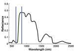
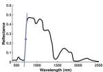
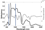
(d) Integral-based indices	(e) Continuum removal	(f) Wavelet transform

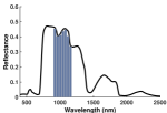
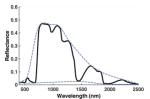
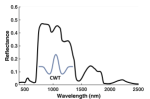
Figure 2: Schematic illustrations of parametric regression methods: Spectral indices (a), Red-edge position (REP) calculation (b), derivative-based indices (c), integral-based indices (d) continuum removal (e), and wavelet transform (f). Note that a fitting function is still required to convert transformations towards a biophysical variable.

3 Non-parametric regression methods

Contrary to parametric methods, non-parametric methods optimize the regression algorithm by means of an inherent learning phase based on training data. Essentially, the non-parametric model develops weights (coefficients) adjusted to minimize the estimation error of the variables extracted. This means that no explicit parametrization is required, which practically simplifies the model development, but more expert knowledge to understand and execute these models may be required. Another important advantage of non-parametric methods is the possibility of training with the full-spectrum information. Hence, an explicit selection of spectral bands or transformations is in principle not required. A flexible model is able to combine different data structure features in a nonlinear manner to conform requirements; however model definition with a too flexible capacity may incur the problem of over-fitting the training dataset. To avoid this pitfall, model weights are defined by jointly minimizing the training set approximation error while limiting the model complexity. In view of processing spectroscopic data, a more prevalent problem lies in the so-called curse of dimensionality (Hughes phenomenon) (Hughes, 1968). Adjacent, contiguous bands carry highly intercorrelated information, which may result in redundant data and possible noise and potentially suboptimal regression performances. As discussed further on, band selection or dimensionality reduction methods that transform the spectral data to lower-dimensional space, while containing the vast majority of the original information can overcome this problem.

Figure 3: Principles of non-parametric regression. Left: RGB subset of a hyperspectral HyMap image (125 bands) over Barrax agricultural site (Spain). Right: illustrative map of a vegetation property (LAI, m²/m²) as obtained by PROSAIL with Gaussian processes regression (GPR). The model was validated with a R² of 0.94 (RMSE: 0.39; NRMSE: 6.3%). It took 5.7 seconds to produce the map using ARTMO’s MLRA toolbox (Rivera Caicedo et al, 2014). With GPR also uncertainty estimates are provided (not shown).

3.1 Linear non-parametric methods

Non-parametric regression algorithms that apply linear transformations are attractive because of their fast performance. These methods became standard methods in chemometric and in image processing software packages. Multivariable linear regression methods can cope with spectroscopic data and typically rely on the estimation of co-variances. When moving towards spectroscopic data, however, this can become problematic when input data quantity is limited with respect to the dimensionality of the dataset. To alleviate collinearity, often linear non-parametric methods are applied in combination with a dimensionality reduction step. Some methods are even intrinsically based on this principle, i.e. principal component regression (PCR) (Wold et al, 1987), and partial least squares regression (PLSR) (Geladi and Kowalski, 1986). Common linear non-parametric regression approaches are provided in table 1 and imaging spectroscopy applications are discussed below.

Table 1: Linear non-parametric regression methods applicable to spectroscopic data.

Method	Description	Ref.
Stepwise multiple linear regression (SMLR)	SMLR recursively applies multiple regression a number of times. Each step removes a variable eliciting the weakest correlation. At the end of the recursive process, a variable set is obtained that is optimally explaining the spectral data distribution.	Draper and Smith (2014)
Principal components regression (PCR)	PCR is a regression analysis method based on principal components analysis (PCA) estimating regression coefficients. Solutions from PCR are generated performing linear regression of the most relevant components (called scores) obtained after applying PCA.	Wold et al (1987)
Partial least squares regression (PLSR)	PLSR is similar as PCR but tackles the co-linearity problem differently than PCR. Applying PCR, regression is performed using PCA scores. These projections are obtained using only input patterns, not outputs. In contrast, PLSR builds the regression model on projections obtained using the partial least squares (PLS) approach. It elicits the directions of maximum input-output cross-covariance. Therefore, PLSR takes both input patterns and output variables into account.	Geladi and Kowalski (1986)
Ridge (regulated) regression (RR)	RR is the most commonly used method of regularization for ill-posed problems, which are problems that do not have a unique solution. RR deals with co-linearity by allowing a degree of bias in the estimates. Therefore, RR adds a small positive value $\lambda$ to the diagonal elements of the input data covariance matrix. Hence, RR requires finding an optimal value for $\lambda$. Typically, cross-validation is used to reach near optimal values. An important fact about RR is that it enforces the regression coefficients to be lower, but it does not enforce them to be zero. That is, it will not get rid of irrelevant features (bands) but rather minimize their impact on the trained model.	Geladi and Kowalski (1986)
Least absolute shrinkage and selection operator (LASSO)	Lasso is an extension built on RR, but with a small twist. It also penalizes the regression coefficients absolute size. By this penalization some of the variable estimates may be exactly zero. The larger the penalty, the more the estimates will tend toward zero. This is a convenient approach to automatically perform feature selection, or to deal with correlated predictors.	Tibshirani (1996)

On the application side, stepwise multiple linear regression (SMLR) is a classical multivariable regression algorithm commonly applied in chemometrics (Atzberger et al, 2010). To evaluate its predictive power, SMLR has been often compared with alternative regression techniques such as PLSR and some studies concluded that PLSR yielded better results when estimating LAI (Darvishzadeh et al, 2008) and canopy chlorophyll content (Atzberger et al, 2010). Also Ramoelo et al (2011) compared both regression algorithms to estimate foliar nitrogen and phosphorus in combination with continuum removal using field spectrometry. By estimating canopy nitrogen, Miphokasap et al (2012) demonstrated that the model developed by SMLR led to a higher correlation coefficient and lower errors than model applications based on narrowband VIs. This suggests that non-parametric (full-spectrum) models tend to be more powerful than parametric models. Likewise, Yi et al (2014) compared SMLR with PLSR and spectral indices for carotenoid estimation in cotton and concluded that best estimations were obtained with PLSR. Likewise, SMLR was compared with PLSR and (nonlinear) machine learning regression algorithms for estimating leaf nitrogen content (Yao et al, 2015). Because of their enhanced flexibility, it may not be a surprise that the nonlinear methods outperformed SMLR and PLSR. This was also observed by various similar studies, as will be addressed in section 3.2.

PCR seems to be more effective in the conversion of spectroscopic data into the estimation of vegetation properties, because the PCA-based dimensionality reduction method is embedded in the method in combination with a linear regression function. Hence, by converting the spectral data to a lower dimensional space automatically overcomes the band redundancy problem. This method has been improved with PLSR, where the projections are optimized in view of the regression. It is, therefore, not a surprise that only few spectroscopic studies examined the predictive power of PCR. Those studies compared PCR against PLSR or against VIs (Atzberger et al, 2010; Fu et al, 2012; Rivera Caicedo et al, 2014; Marshall and Thenkabail, 2014; Wang et al, 2017b). Although PCR generally outperformed VIs in explaining variability of a vegetation attribute, in all cases PLSR or any other non-parametric method overran PCR.

PLSR found its way in a broad diversity of imaging spectroscopy applications, especially in the mapping of biochemicals, pigments and vegetation density properties. For instance, PLSR was used in several spectroscopic studies applied to estimate foliage nitrogen content (Hansen and Schjoerring, 2003; Coops et al, 2003; Huang et al, 2004). Also Gianelle and Guastella (2007) used PLSR to derive grassland phytomass and its total (percentage) nitrogen content from spectroscopic data. Similarly, Cho et al (2007) and Im et al (2009) applied PLSR to estimate a diversity of grass and crop biophysical variables (LAI, stem biomass and leaf nutrient concentrations), and Ye et al (2007) applied PLSR for yield prediction purposes. Beyond individual vegetation attributes, PLSR was recently used to predict landscape-scale fluxes of net ecosystem exchange (NEE) and gross primary productivity (GPP) across multiple timescales (Matthes et al, 2015), and also for the estimation of floristic composition of grassland ecosystems (Harris et al, 2015; Roth et al, 2015; Neumann et al, 2016). At the same time, thanks to its PLS-vectors, PLSR is also increasingly applied for band sensitivity analysis of spectroscopic datasets in view of the targeted application (e.g. Li et al, 2014a; Feilhauer et al, 2015; Neumann et al, 2016; Kiala et al, 2016; Kira et al, 2016). Various experimental studies demonstrated the superior predictive power of PLSR as opposed to VIs for the prediction of multiple vegetation properties, including above-ground biomass, LAI, leaf pigments (chlorophyll, carotenoids), GPP and NEE fluxes, leaf rust disease detection and nutrients concentration (nitrogen and phosphorus concentrations) (Hansen and Schjoerring, 2003; Dreccer et al, 2014; Capolupo et al, 2015; Matthes et al, 2015; Foster et al, 2017; Yue et al, 2017; Wang et al, 2017a). However, when compared against machine learning methods, then PLSR no longer appeared to be top performing (Yao et al, 2015; Wang et al, 2015; Kiala et al, 2016; Ashourloo et al, 2016). As will be addressed in section 3.2, this is due to the nonlinear transformation conducted in machine learning methods.

Other linear non-parametric regression methods, such as ridge regression (RR) and LASSO, hardly made it into applications for vegetation properties mapping. Yet a few spectroscopic examples are worth mentioning. For instance, Addink et al (2007) used RR to map LAI and biomass, and more recently Bratsch et al (2017) applied LASSO to estimate above-ground biomass quantities among different plant tissue type categories in Alaska. In another biomass estimation study, both RR and LASSO were compared against PLSR (Lazaridis et al, 2010) and also random forests (Zandler et al, 2015). Interestingly, RR and LASSO appeared to be top performing. One may, therefore, wonder why these techniques have not been applied more often. On the other hand, these linear methods are increasingly replaced by their nonlinear counterparts. For instance, RR has been replaced by kernel ridge regression (KRR) (Suykens and Vandewalle, 1999), and also PLSR has been redesigned into a kernel version, i.e. the KPLSR, which proved to be more powerful than PLSR for chlorophyll concentration estimation (Arenas-García and Camps-Valls, 2008). The family of kernel methods is addressed in section 3.2. That none of these linear methods deliver uncertainty estimates is another drawback. Similar as in case of parametric regression, without uncertainty estimates it remains questionable whether these methods can deliver consistent mapping quality throughout a complete image, or are applicable to other images in space and time.

(a) PCR	(b) PLSR	(c) RR & LASSO

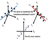
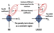
Figure 4: Schematic illustrations of principal component (PC) (a), partial least squares (PLS) (B), ridge regression and LASSO (c). PC and PLS is combined with a linear regression model.

3.2 Nonlinear non-parametric models

When advancing beyond linear transformation techniques, a diversity of nonlinear non-parametric models has been developed during last few decades. These methods, also referred to as machine learning regression algorithms, apply nonlinear transformations. An important methodological advantage is their capability to capture nonlinear relationships of image features without explicitly knowing the underlying data distribution. Hence, they are developed without assuming a particular probability density distribution, which is the reason why they work well with all kinds of data types. Machine learning methods also offer the possibility to incorporate a prior knowledge and the flexibility to include different data types into the analysis. In principle they are perfectly suited to process spectroscopic data. In the following sections, examples of the families of (1) decision trees, (2) artificial neural networks and (3) kernel-based regression are explained.

3.2.1 Decision trees

Table 2: Decision tree regression methods applicable to spectroscopic data.

Method	Description	Ref.
Decision trees (DT)	DT learning is based on decision tree predictive modeling. A decision tree is based on a set of hierarchical connected nodes. Each node represents a linear decision based on a specific input feature.	Breiman et al (1984)
Boosted trees (BoT)	BoT Incrementally builds an ensemble by training each new instance to emphasize the training instances previously mis-modeled.	Friedman et al (2000)
Bagging trees (BaT)	BaT an early ensemble method based on building multiple decision trees by iteratively replacing resampled training data and voting for the decision trees leading to a consensus prediction.	Breiman (1996)
Random Forests (RF)	RF is a specific type of BaT that in constructs a collection of decision trees with controlled variance.	Breiman (2001)

Decision tree algorithms use a branching method to illustrate every possible outcome of a decision (for examples see Table 2). They are more frequently applied in classification than in regression. Only a few decision tree feasibility studies dealing with imaging spectroscopy data are presented in the scientific literature (e.g. Im et al, 2009) most likely because boosted and bagging trees hardly found their way to regression applications. They might be considered as obsolete with the improvements introduced into random forests (RF), which is essentially a specific type of bagging trees. RF builds an ensemble of individual decision trees working with different subsets of features (bands) and eventually different training data points both selected randomly, from which a final prediction is made using particular combination schemes. RF can handle a large number of training samples, does not suffer from overfitting and is robust to outliers and noise (Belgiu and Drăguţ, 2016), which makes it an attractive method for spectroscopic mapping applications. RF has recently been made available in various software packages and proved to be a competent regression algorithm. It therefore comes as no surprise that RF gained rapid popularity in imaging spectroscopy mapping of a diverse range of vegetation attributes, including biomass (Adam et al, 2014; Vaglio Laurin et al, 2014), canopy nitrogen (Li et al, 2014b) and as indicator of plant species composition (Feilhauer et al, 2017). Some of these studies have compared RF with support vector regression (SVR) or neural networks, but no strong preference towards one or the other method was found, which suggests that all three methods are competitive (Han et al, 2016; Pullanagari et al, 2016). However, just like other machine learning regression methods, RF can face difficulties coping with the collinearity of the spectroscopic data (Rivera-Caicedo et al, 2017). To overcome this problem, RF is often used in combination with sensitive bands or simple transformations in the form of VIs that are known to be sensitive to the targeted vegetation property (Adam et al, 2014; Liang et al, 2016; Han et al, 2016). Alternatively, RF is inherently able to identify sensitive spectral bands, and selection of only those sensitive bands can subsequently improve the regression model (Feilhauer et al, 2015; Balzarolo et al, 2015). Whether applying a band selection method is the most successful strategy, however, remains an open question. Rather than seeking for optimized individual bands, a more elegant solution may lie in firstly applying dimensionality reduction method, and then inputting the features of the lower-dimensional space (i.e., components) into the decision tree (Rivera-Caicedo et al, 2017).

3.2.2 Artificial neural networks

Table 3: Artificial neural network regression methods applicable to spectroscopic data.

Method	Description	Ref.
Artificial neural networks (ANN)	ANNs in their basic form are essentially fully connected layered structures of artificial neurons (AN). An AN is basically a pointwise nonlinear function (e.g., a sigmoid or Gaussian function) applied to the output of a linear regression. ANs with different neural layers are interconnected with weighted links. The most common ANN structure is a feed-forward ANN, where information flows in a unidirectional forward mode. From the input nodes, data pass hidden nodes (if any) toward the output nodes.	Haykin (1999)
Back-propagation ANN (BPANN)	The he basic type of neural network is multi-layer perceptron, which is feed-forward back-propagation ANN. BPANN consists of 2 steps: 1) feed forward the values, and 2) calculate the error and propagate it back to the earlier layers. So to be precise, forward-propagation is part of the backpropagation algorithm but comes before back-propagating. This is the most common used algorithm when referring to ANN. In many papers using ANN these standard designs are not explicitly mentioned.	Haykin (1999)
Radial basis function ANN (RBFANN)	RBFANN is a type of ANN that uses non-linear radial basis functions (RBF) as activation functions in the hidden layer. The output of the network is a linear combination of RBFs of the inputs and neuron parameters.	Broomhead and Lowe (1988)
Recurrent ANN (RANN)	A RANN is a type of ANN that make use of sequential information by introducing loops in the network.	Hochreiter and Schmidhuber (1997)
Bayesian regularized ANN (BRANN)	BRANNs are more robust than standard BPANNs and can reduce or eliminate the need for lengthy cross-validation. Bayesian regularization is a mathematical process that converts a nonlinear regression into a "well-posed" statistical problem in the manner of a ridge regression.	Burden and Winkler (1999)

Artificial neural networks (ANNs) methods are listed in table 3. Since the early 90s, feed-forward and back-propagation ANNs thrived in all kinds of mapping applications, including vegetation properties mapping (Paruelo and Tomasel, 1997; Francl and Panigrahi, 1997; Kimes et al, 1998). Their strengths lie in their adaptability that can lead to excellent performances. The superiority of ANNs in vegetation properties mapping compared to parametric models (e.g. those based on VIs) has been demonstrated repeatedly in experimental studies (Uno et al, 2005; Wang et al, 2013; Malenovský et al, 2013; Kalacska et al, 2015). Examples of successful spectroscopic applications include the estimation of foliage nitrogen concentrations (Huang et al, 2004) and LAI (Jensen et al, 2012; Neinavaz et al, 2016). In both cited studies, ANN outperformed other linear non-parametric models (e.g. PLSR). Alternative powerful structures involve RBFANNs, BRANNs and RANNs (for explanation see table 3). Although these advanced ANNs have been primarily used for classification applications, only recently they were explored to map vegetation properties from spectroscopic data (Wang et al, 2013; Chen et al, 2015; Feng et al, 2016; Pôças et al, 2017). Some of these studies mention the superiority of these advanced ANN designs as compared to standard ANN designs or other machine learning approaches in estimating vegetation properties (Du et al, 2016; Pham et al, 2017; Li et al, 2017).

Applying ANNs to spectroscopic data, nonetheless, can be quite challenging due to the multicollinearity. Feeding many bands into an ANN requires a complex design and consequently a long training time. Just as with decision trees, a popular approach is applying a band selection or the calculation of several sensitive VIs or shape indices such as red edge position that are then entered either individually or as a combination into the ANN. Various of these band selection studies investigated combinations of VIs that led to best prediction models (Schlerf and Atzberger, 2006; Mutanga and Kumar, 2007; Jia et al, 2013; Chen et al, 2015; Liang et al, 2015; Feng et al, 2016; Pôças et al, 2017). As discussed before, it remains questionable whether the selected indices preserve a maximum amount of useful information. In contrary, when compressing the spectral data using dimensionality reduction methods into a lower-dimensional space, then it is ensured that a maximum amount of spectral information is preserved. This approach was applied e.g. to assess corn yield (Uno et al, 2005) and phosphorus and nitrogen concentrations (Knox et al, 2011). It is therefore not surprising that a study comparing PCA vs. indices inputted into ANNs concluded that the PCA-ANN design outperformed VI-ANN designs (Liu and Pan, 2017). Moreover, given that only linear transformations are applied in PCA, it may even be that more adaptive dimensionality reduction methods yield superior accuracies when combined with ANN, e.g. partial least squares (PLS), or in the field of nonlinear kernel-based dimensionality reduction methods, e.g. kernel PCA (KPCA) or kernel PLS (KPLS). To ascertain this hypothesis, PCA was compared against 10 alternative dimensionality reduction methods in combination with ANN to carry out LAI estimation. As expected, various alternative dimensionality reduction methods outperformed PCA in developing accurate models (e.g., PLS, KPLS, KPCA) (Rivera-Caicedo et al, 2017).

3.2.3 Kernel-based machine learning regression methods

Table 4: Kernel-based regression methods applicable to spectroscopic data.

Method	Description	Ref.
Support vector regression (SVR)	The Support Vector Machine (SVM) is a supervised machine learning technique that was invented in the context of the statistical learning theory. It was not until the mid-90s that an algorithm implementation of the SVM was proposed with the introduction of the kernel trick and the generalization to the non-separable case. SVR is built on the principle of SVM: a non-linear function is learned by linear learning machine mapping into high dimensional kernel induced feature space. The capacity of the system is controlled by parameters that do not depend on the dimensionality of feature (bands) space.	Vapnik et al (1997)
Kernel ridge regression (KRR)	KRR combines RR with the kernel trick. It thus learns a linear function in the space induced by the respective kernel and the data. For non-linear kernels, this corresponds to a non-linear function in the original space. The form of the model learned by KR is identical to SVR. However, different loss functions are used: KRR uses squared error loss while SVR uses $\epsilon$-insensitive loss combined with RR regularization.	Suykens and Vandewalle (1999)
Gaussian process regression (GPR)	GPR is based on Gaussian processes (GPs), which generalize Gaussian probability distributions in a function’s space. A GP is stochastic since it describes the properties of functions. As in Gaussian distributions, a GP is described by its mean (which for GPs is a function) and covariance (a kernel function). This represents an expected covariance between function values at a given point. Because a GPR model is probabilistic, it is possible to compute the prediction intervals using the trained model.	Rasmussen and Williams (2006)

Kernel-based regression methods solve nonlinear regression problems by transferring the data to a higher-dimensional space by a kernel function (Table 4). The flexibility offered by kernel methods allows to transform almost any linear algorithm that can be expressed in terms of dot products, while still using only linear algebra operations. Kernel methods provide a consistent theoretical framework for developing nonlinear techniques and have useful properties when dealing with a low number of (potentially high dimensional) training samples, and outliers and noise in the data (Gómez-Chova et al, 2011; Tuia et al, 2018). Given these attractive properties, kernel-based regression methods seem perfectly suited to extract nonlinear information related to vegetation properties from imaging spectroscopy data. Developed in the mid-90s, among the most popular kernel-based method for classification purposes involves SVMs. Its regression version (SVR) gained popularity for the retrieval of continuous vegetation attributes from imaging spectroscopy data in the last decade. Examples include plant height, leaf nitrogen content, and leaf chlorophyll content (Karimi et al, 2008; Yang et al, 2011). A multi-output version of SVR was presented by Tuia et al (2011), with LAI, leaf chlorophyll content and fractional vegetation content being simultaneously estimated. Recently, SVR was used for processing spectroscopic images of sub-decimeter spatial resolution as acquired by low-altitude unmanned aircraft system to infer Antarctic moss vigour (Malenovský et al, 2017). Yet just as with the other advanced regression methods, SVR face the same difficulties of coping with multicollinearity. Therefore, SVR has been commonly applied in combination with specific spectral subsets or VIs (Marabel and Alvarez-Taboada, 2013; Lin et al, 2013), or with wavelet transforms (He et al, 2015). To deal with spectroscopic band redundancy, an advantage of SVR is that it allows band selection (analogous as PLSR and RF), which in principle allows the development of more optimized models (Feilhauer et al, 2015). On the other hand, it is likely that the combination with dimensionality reduction methods will lead to more powerful models (Rivera-Caicedo et al, 2017). To assess its predictive power, various spectroscopic studies compared SVR against similar methods such as SMLR or PLSR, although some band selection method appeared to be essential (Wang et al, 2015; Yao et al, 2015; Kiala et al, 2016). Conversely, when comparing SVR against other machine learning methods such as RF or GPR, then SVR no longer excelled (Pullanagari et al, 2016).

Kernel ridge regression (KRR) emerged as one of the promising upcoming kernel-based regression methods, although only a few spectroscopic studies have used it. For instance, Wang et al (2011) compared KRR with linear non-parametric methods (multiple linear regression and PLSR) for LAI estimation. The authors concluded that KRR yielded the most accurate estimates. Also Peng et al (2011) used KRR for the detection of chlorophyll content. Apart from these two studies, the spectroscopy vegetation community may not yet be familiar with this method. Solely Rivera Caicedo et al (2014) had compared KRR against other machine learning algorithms applied to CHRIS (62 bands) and HyMap (125 bands) spectroscopic data for LAI mapping. In that study, KRR not only proved to be a very competitive regression algorithm, but also proved to be extremely fast. This is due to its relatively simple design that requires only one hyperparameter to be tuned. Because of its simplicity, another advantage is that KRR is capable to deal with collinearity; the method can cope with thousands of contiguous bands. In fact, in the dimensionality reduction comparison study tested with simulated (2100 bands) and HyMap data (Rivera-Caicedo et al, 2017), KRR was the only regression method where dimensionality reduction methods did not lead to improvements as compared to using all bands. In conclusion, KRR emerged as an attractive regression method due to its competitive performance, fast processing and easiness to deal with spectroscopic data.

From all machine learning regression algorithms, probably the most exciting one is Gaussian process regression (GPR). Contrary to other methods, the training phase in GPR takes place in a Bayesian framework, leading to probabilistic outputs (Rasmussen and Williams, 2006; Camps-Valls et al, 2016). GPR applied to spectroscopic data started only recently, e.g. for airborne HyMap mapping of leaf chlorophyll content (Verrelst et al, 2013a), and for spaceborne CHRIS mapping of leaf chlorophyll content, LAI and fractional vegetation content (Verrelst et al, 2012a). Of interest is that along with these maps also maps of associated uncertainties (prediction intervals) were provided. Also with an Airborne Hyperspectral Scanner (Roelofsen et al, 2014) applied GPR to map salinity, moisture and nutrient concentrations that in turn were used as inputs for plant association mapping. In the Rivera Caicedo et al (2014) comparison paper, GPR outperformed the majority of other tested machine learning methods for the prediction of leaf chlorophyll content and LAI from various spectroscopic datasets. Similarly, Ashourloo et al (2016) concluded that GPR yielded most accurate leaf rust disease detection as compared to VIs, PLSR and SVR. However, GPR is no exception in suffering from radiometric collinearity when many bands are included; and related spectroscopic studies demonstrated that results can be further improved by combining GPR with band selection (Verrelst et al, 2016b) or with dimensionality reduction methods (Rivera-Caicedo et al, 2017). At the same time, alternative GPR versions continue to be developed within the machine learning community. For instance, Lazaro-Gredilla et al (2014) refined the GPR method by proposing a non-standard variable approximation allowing for accurate inferences in signal-dependent noise scenarios. The so-called variational heteroscedastic GPR (VHGPR) appears to be an excellent alternative for standard GPR, which was demonstrated on a CHRIS dataset where VHGPR outperformed GPR in leaf chlorophyll content estimation.

(a) RF	(b) NN	(c) SVR	(d) GPR

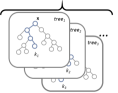
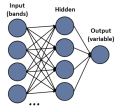
Figure 5: Schematic illustrations of Random forest (RF) (a), Neural networks (NN) (b), Support vector regression (SVR) (c), and Gaussian processes regression (GPR) (d).

4 Physically-based model inversion methods

Physically-based model inversion is based on physical laws establishing cause-effect relationships. Inferences on model variables are based on generally accepted knowledge embedded in radiative transfer models (RTMs). RTMs are deterministic models that describe absorption and multiple scattering, and some of them even describe the microwave region, thermal emission or sun-induced chlorophyll fluorescence emitted by vegetation (e.g., see Table 5). A diversity of canopy RTMs have been developed over the last three decades with varying degrees of complexity. Gradual increase in RTMs accuracy, yet in complexity too, have diversified RTMs from simple turbid medium RTMs to advanced Monte Carlo RTMs that allow for explicit 3D representations of complex canopy architectures (e.g., see the RAMI exercises (Pinty et al, 2001, 2004; Widlowski et al, 2007, 2011, 2015) for a thorough comparison). This evolution has resulted in an increase in the computational requirements to run the model, which bears implications towards practical applications. From a computational point of view, RTMs can be categorized as either (1) economically invertible (or computationally cheap); or as (2) non-economically invertible models (or computationally expensive). These terms refer to the model complexity and associated run-time constraining the mathematical inversion of such models. Economically invertible models are models with relatively few input parameters and fast processing that enables fast calculations and consequently fast model inversion or rendering of simulated scenes. A well-known example of this category includes the widely used leaf RTM PROSPECT (Feret et al, 2008) coupled with the canopy RTM SAIL (Verhoef, 1984a) (combined named as PROSAIL (Jacquemoud et al, 2009a)).

Non-economically invertible RTMs refer to advanced, computationally-expensive RTMs, often with a large number of input variables and sophisticated computational and mathematical modelling. These type of RTMs enable the generation of complex or detailed scenes, but at the expense of a significant computational load. In short, the following families of RTMs can be considered as non-economically invertible: (1) Monte Carlo ray tracing models (e.g., Raytran (Govaerts and Verstraete, 1998), FLIGHT (North, 1996) and librat (Lewis, 1999)); (2) voxel-based models (e.g., DART (Gastellu-Etchegorry et al, 1996)) and (3) advanced integrated vegetation and atmospheric transfer models (e.g., SCOPE (Van Der Tol et al, 2009) and MODTRAN (Berk et al, 2006)). Descriptions of advanced canopy RTM models and their latest developments are provided in Table 5. Although these advanced RTMs serve perfectly as virtual laboratories for fundamental research on light-vegetation interactions, they are in general less suitable for retrieval applications, because of either a large number of input variables or a long processing time. Nevertheless, as outlined below, some experimental studies demonstrated that they can as well be applied into inversion schemes, e.g. based on look-up tables and in hybrid strategies.

Regardless of their complexity, they all deliver spectroscopic outputs, typically at 1 nm resolution. Hence, RTMs outputs can fit perfectly into inversion schemes of imaging spectroscopy data, while at the same time the simulated data can be resampled to reassemble the band settings of multispectral sensors. Because inversion strategies are usually based on spectral fitting (i.e. only radiometric information is used), the drawback of collinearity complicating regression is not an issue here; however, removal of noisy bands is still a standard and much-needed preprocessing step to enable adequate spectral fitting. Another point to be mentioned is that inversion scheme can only retrieve the RTM input variables. Hence, using this strategy implies that only RTM state variables can be mapped. Yet because the RTM input variables drive the canopy absorbance and scattering mechanisms, the resulting output maps are considered to be physically sound (Myneni et al, 1995; Knyazikhin et al, 2013).

Figure 6: Principles of RTM inversion. Left: RGB subset of a hyperspectral HyMap image (125 bands) over Barrax agricultural site (Spain). Right: illustrative map of a vegetation property (LAI, m²/m²) as obtained by RMSE inversion against a 100000 PROSAIL LUT (5% noise added, mean of 5% multiple solutions). The model was validated with a R² of 0.44 (RMSE: 1.85; NRMSE: 31.9%). A systematic underestimation occurred, which in principle implies that the RTM simulated LUT needs to be better parameterized.

It took 2315 seconds to produce the map using ARTMO’s LUT-based inversion toolbox (Rivera et al, 2013). Also uncertainty estimates are provided, e.g. in the form of residuals (not shown).

Table 5: Advanded canopy RTMs commonly used in imaging spectroscopy applications.

RTM	Description
SCOPE(Soil-Canopy-Observation of Photosynthesis and Energy fluxes)	SCOPE (Van Der Tol et al, 2009) is a Soil-Vegetation-Atmosphere (SVAT) scheme that includes RTMs along with a micrometeorological model for simulating turbulent heat exchange, and a plant physiological model for photosynthesis (Van Der Tol et al, 2014). The radiative transfer scheme is based on SAIL (Verhoef, 1984b, 1985), extended with a similar radiative transfer for emitted radiation. The emitted radiation includes chlorophyll fluorescence and thermal radiation. Leaf radiative transfer is calculated with Fluspect (Vilfan et al, 2016) which also includes emitted fluorescence radiation. SCOPE is intended as tool to scale processes from leaf to canopy, and to analyse the effects of light scattering. Recent developments include vertical heterogeneity (Yang et al, 2017) and the zeaxanthin-violaxanthin pigment cycles.
Discrete Anisotropic Radiative Transfer (DART)	DART model is being developed since 1992 as a physically based 3D computer programme (Gastellu-Etchegorry et al, 1996), which simulates radiative budget and remote sensing (airborne and space-borne) optical image data of natural and urban landscapes for any wavelengths from the ultraviolet to the thermal infrared part of the electromagnetic spectrum (Gastellu-Etchegorry et al, 1999; Guillevic et al, 2003). It computes and provides bottom and top of the atmosphere spectral quantities (i.e., irradiance, exitance and radiance) that are transformed into reflectance or brightness temperature depending on the user DART mode preferences (Gastellu-Etchegorry et al, 2004). Simulated scenes may include the atmosphere, topography and any natural or anthropogenic objects at any geographical location (Grau and Gastellu-Etchegorry, 2013). The latest DART optical development includes also the specular reflectance and the light polarization (Gastellu-Etchegorry et al, 2015). Apart of passive remote sensing data, it also simulates active terrestrial and air-/space-borne light detection and ranging (LiDAR) discrete return, full waveform, multi-pulse and photon counting measurements (Gastellu-Etchegorry et al, 2016; Yin et al, 2016). In case of vegetation, it can also simulate radiative transfer of the solar-induced chlorophyll fluorescence for any virtual 3D Earth scene numerically and as images (Gastellu-Etchegorry et al, 2017).
librat	librat is a 3D Monte Carlo ray tracing radiative transfer model developed as a library interface to the original ararat (Advanced RAdiometric RAy Tracer) model. The first version of ararat was published in 1992 (Lewis and Muller, 1993) as part of the Botanical Plant Modelling System (BPMS) (Lewis and Muller, 1990; Lewis, 1999). Subsequently, the sampling scheme was improved as reported in Saich et al (2002), and the codes developed into a library in recent years. librat reads a 3D description of (canopy/soil/topographic) geometry, along with associated information on material scattering properties. The main function in the library then is that a ray is launched from some origin in 3D space, in a specified direction, and the code returns all information about the associated scattering paths and interactions, separated as direct and diffuse components. This core functionality, along with a set of associated sensor models but integrating paths fired into some volume. It allows for a wide range of radiative transfer calculations, including time-resolved/lidar, splitting of the radiometric information per scattering order etc. as well as straightforward raflectance/transmittance calculations (e.g. Disney et al, 2006; Hancock et al, 2012).
FLIGHT	FLIGHT (North, 1996; Barton and North, 2001) is a Monte Carlo ray tracing model designed to rapidly simulate light interaction with 3D vegetation canopies at high spectral resolution, and produce reflectance spectra for both forward simulation and for use in inversion (Leonenko et al, 2013). Foliage is represented by structural properties of leaf area, leaf angle distribution, crown dimensions and fractional cover, and the optical properties of leaves, branch, shoot and ground components. The model represents multiple scattering and absorption of light within the canopy and with the ground surface. It has been developed to model 3D canopy photosynthesis (Alton et al, 2007), to simulate waveform and photon counting lidar (North et al, 2010; Montesano et al, 2015) and emitted fluorescence radiation (Hernández-Clemente et al, 2017). Structural data may be specified as a statistical distribution, derived from field measurements (Morton et al, 2014) or by direct inversion from LiDAR data (Bye et al, 2017).

Given that in principle only a coupled leaf-canopy RTM and an inversion routine are required for the retrieval of RTM state variables, the approach is generic and generally applicable. Nevertheless, these approaches are not straightforward. First, an RTM has to be selected, whereby a trade-off between the realism and inversion possibility of the RTM has to be made. As discussed above, typically, complex models are more realistic, but they have many variables and consequently challenging to invert, whereas simpler models may be less realistic but easier to invert. Secondly, according to the Hadamard postulates, RTMs are invertible only when an inversion solution is unique and dependent – in a continuous mode – on the variables to be extracted. Unfortunately, this boundary condition is often not met. The inversion of canopy RTMs is frequently under-determined and ill-posed. The number of unknowns can be much larger than the number of independent observations. This makes physically-based retrievals of vegetation properties a challenging task. Several strategies have been proposed to cope with the under-determined problem of optimizing the inversion process, including (1) iterative numerical optimization methods, (2) lookup-table (LUT) based inversion, or (3) hybrid approaches in which LUTs are generated as input for machine learning approaches (see section 5). Below we briefly review some common RTM inversion techniques in view of converting spectroscopic data into maps of RTM leaf and canopy input variables.

Numerical optimization: Iterative optimization is a classical technique to invert RTMs in image processing (Jacquemoud et al, 1995; Zarco-Tejada et al, 2001; Botha et al, 2007). The optimization is minimizing a cost function, which estimates the difference between measured and estimated variables by successive input variable iteration. Optimization algorithms are computationally demanding and hence potentially time-consuming depending on the complexity of the RTM and the numbers of image pixels to be processed. However, with the ongoing increase in computational power and open-source availability of optimization libraries, a renaissance of numerical approaches is emerging. Examples of numerical inversion against spectroscopic data include: PROSPECT inversion to retrieve leaf chlorophyll content (Zhang and Wang, 2015), retrieval of leaf biochemistry against an improved version of PROSPECT (COSINE) (Jay et al, 2016), and PROSAIL leaf and canopy variables (Bayat et al, 2016; van der Tol et al, 2016). Despite a gain in computational power, numerical inversion algorithms applied to images are still time-consuming given the many per-pixel iterations and a high number of pixels involved. Hence, in its current form this method stays restricted to computationally fast RTMs in merely experimental settings.

Look-up table (LUT) strategies are based on the generation of simulated spectral reflectance scenarios for a high number of plausible combinations of variable value ranges. As such, the inversion problem is reduced to the identification of the modeled reflectance set that resembles most closely the measured one. This process is based on querying the LUT and applying a cost function. A cost function minimizes the summed differences between simulated and measured reflectances for all wavelengths. The main advantage of LUT-based inversion routines over numerical optimization is their computational speed, since the computationally most demanding part of the inversion procedure is completed before the inversion itself (Dorigo et al, 2007). Consequently, LUT-based inversion methods are typically used as a preferred solution in RTM inversion studies. The classical LUT-based inversion approach is based on a RMSE cost function, which continues to be applied until today. This approach proved to be especially successful for chlorophyll (Zhang et al, 2008; Kempeneers et al, 2008; Omari et al, 2013) and LAI mapping. For instance, by using LUT-based inversion routines imaging spectroscopy data has been processed for the mapping of forest LAI (Banskota et al, 2013, 2015), grassland LAI (Atzberger et al, 2015) and LAI over agricultural crops based on UAVs (Duan et al, 2014). To further mitigate the ill-posed problem and optimize the robustness of the LUT-based inversion routines, a diversity of regularization strategies have been explored in inversion applications against spectroscopic data:

• The use of prior knowledge to constrain model variables in the development of a LUT (Koetz et al, 2005; Darvishzadeh et al, 2008; Baret and Buis, 2008). Prior knowledge typically involves information on the feasible variable ranges for involved vegetation types (Dorigo et al, 2009; Verrelst et al, 2012c). Prior information together with prior distributions are also increasingly applied into a Bayesian context, whereby the inverted values are generated based on likelihoods (Laurent et al, 2013, 2014; Shiklomanov et al, 2016). The advantage of a Bayesian framework is its capability to quantify an inversion uncertainty around an inversion variable.

• Selection of cost function. The inverse problem of a nonlinear RTM is based on the minimization of a cost function concurrently measuring the discrepancy between (i) observed and simulated reflectance, and (ii) variables to estimate and the associated prior information (Jacquemoud et al, 2009b). To avoid solutions reaching fixed boundaries, a modified cost function in the LUT search that takes uncertainty of provided prior information into account is sometimes used, e.g. by means of the above-mentioned Bayesian approach. Alternatively, Leonenko et al (2013) proposed and evaluated over 60 different cost functions dealing with different error distributions. Some more spectroscopic studies have evaluated among others the role of cost function (Locherer et al, 2015; Danner et al, 2017) in LUT-based inversion. Although the classical RMSE is a robust cost function, sometimes improvements can be gained with alternative cost functions, e.g. when the LUTs are non-normal distributed.

• The use of multiple best solutions in the inversion (mean or median), as opposed to a single best solution (Koetz et al, 2005; Locherer et al, 2015; Banskota et al, 2015; Kattenborn et al, 2017).

• The addition of artificial noise (additive or inverse multiplicative white noise) to account for uncertainties linked to measurements and models (Koetz et al, 2005; Locherer et al, 2015; Danner et al, 2017).

• Several spectroscopic studies reported that the relationship between measured and estimated variable perceptibly improves when only specific (sensitive) spectral ranges are selected for model inversion (Meroni et al, 2004; Schlerf et al, 2005; Darvishzadeh et al, 2012). To account for noise in the observations, other spectroscopic studies instead manipulated the observed spectra by applying a smoothing filter (Arellano et al, 2017) or wavelet transforms (Banskota et al, 2013; Ali et al, 2016; Kattenborn et al, 2017). Spectral selection and spectral polishing methods can be applied at the same time in order to enhance the resemblance with the usually more spectrally smooth simulated spectra.

Because of taking sun-target-sensor geometry into account, the use of RTM-based methods has been demonstrated to improve robustness to solar and view angle effects, compared to index-based methods (Kempeneers et al, 2008). Another advantage of RTM inversion routines is that uncertainties are provided as spectral residuals (Rivera et al, 2013) or standard deviations, when mapping multiple solution means (Verrelst et al, 2014). Yet the main drawback lies in its computational burden resulting from too many per-pixel iterations. Although LUT-inversion approaches may speed-up the inversion process as opposed to numerical inversion, these inversion routines are still computationally expensive due to the iterative calls of LUT entries on a per-pixel basis. Consequently, despite attempts to optimize inversion algorithms in order to save-up computational time for solving inverse radiative transfer problems (Gastellu-Etchegorry et al, 2003; Favennec et al, 2016), in terms of processing speed the RTM inversion routines run still behind statistical methods.

(a) Numerical inversion	(b) LUT-based inversion

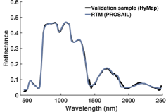
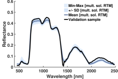
Figure 7: Examples of numerical inversion (a) and LUT-based inversion (b). A HyMaP spectrum was inverted against PROSAIL. In case of LUT-inversion, overview statistics of 5% best multiple solutions are shown.

5 Hybrid regression methods

Having discussed the more fundamental categories of retrieval methods, this section addresses hybrid regression methods. Hybrid methods combine the generalization level of physically-based methods with the flexibility and computational efficiency of advanced machine learning methods. This approach replaces the ground data needed for training of the parametric or non-parametric models by RTM input variables, which makes it computationally efficient. It is important to note that the hybrid approach does not alleviate the main issues of RTMs, notably that they only include existing knowledge and concepts. Similarly as in case of LUT-based inversion, RTM simulations build a LUT representing a broad set of canopy realizations and the hybrid approach uses all available data stored in LUT to train a machine learning regression model.

Figure 8: Principles of hybrid regression. Left: RGB subset of a hyperspectral HyMap image (125 bands) over Barrax agricultural site (Spain). Right: illustrative map of a vegetation property (LAI, m²/m²) as obtained by PROSAIL with Gaussian processes regression (GPR) and 15% white noise added. The model was validated with a R² of 0.88 (RMSE: 0.70; NRMSE: 10.1%)

. It took 6.3 seconds to produce the map using ARTMO’s MLRA toolbox (Rivera Caicedo et al, 2014). With GPR also uncertainty estimates are provided (not shown). Because not being trained with bare soil spectra, LAI over the non-irrigated parcels is overestimated.

The awareness in the mid 90’s that ANNs are excellent algorithms to deal with large datasets led to the introduction of hybrid methods based on ANNs trained with generically applicable RTM-generated data. It led to operational retrieval algorithms for datastreams acquired by multispectral and superspectral sensors (see Verrelst et al (2015)). Although this approach is less straightforward in the context of imaging spectroscopy, because of the challenge of collinearity, some recent efforts have been undertaken in exploring this research direction. Noteworthy is the work of Vohland et al (2010) comparing a numerically optimized ANN with a LUT-based inversion using PROSAIL RTM simulations. Prediction accuracies generally decreased in the following sequence: numerical optimization > LUT > ANN. This would indicate that an ANN may not always be the best choice for inversion applications. However, no dimensionality reduction method was applied, which suggests that the regression model suffered from band collinearity effects. Also Fei et al (2012) compared a PROSAIL-ANN hybrid approach with a PCA approach. The authors concluded that a PCA transformation into a regression function can mitigate the known reflectance saturation effect of dense canopies to some extent. This PROSAIL-ANN strategy was revisited by Rivera-Caicedo et al (2017) with alternative dimensionality reduction methods. Although PCA improved accuracies as opposed of using all bands, substantially more improvements were achieved when converting the spectra into components by means canonical correlation analysis (CCA) or orthonormalized PLS (OPLS).

Likewise, inputs from more advanced RTMs were explored to develop specialized hybrid structures. In Malenovský et al (2013) an ANN was trained based on PROSPECT-DART simulations that explicitly took 3D canopy structures into account to estimate forest leaf chlorophyll content from hyperspectral airborne AISA data. In this approach the DART simulations went first through a continuum removal transformation. Alternatively, some studies have attempted to move away from ANN models by exploring hybrid structures on the basis of kernel-based machine learning regression algorithms, particularly the popular SVR. For instance, leaf chlorophyll content was estimated based on a PROSAIL-SVR model and applied to imaging spectroscopy (Preidl and Doktor, 2011). An analogous concept was applied for a SVR that was trained by PROSPECT-DART simulations in combination with continuum removal transformations, with the purpose of quantifying forest biochemical and structural properties (Homolová et al, 2016). Similarly, Doktor et al (2014) used a PROSAIL dataset to train a random forests (RF) model to predict LAI and leaf chlorophyll content, and Liang et al (2016) compared PROSAIL-based hybrid models with SVR and RF for leaf and canopy chlorophyll content estimation from CHRIS data. Finally, (Rivera-Caicedo et al, 2017) analyzed ensembles of regression algorithms with dimensionality reduction methods to consolidate the most ideal PROSAIL-based (2101 bands) hybrid regression model. This study concluded that compressing PROSAIL data into CCA or OPLS components led to highest accuracies when trained with a GPR model. Altogether, although these studies have only been developed in experimental settings – similar as the operational multispectral hybrid algorithms (e.g. Bacour et al, 2006; Baret et al, 2013) – the hybrid structures can be perfectly implemented into global mapping schemes. When combined with a dimensionality reduction method to suppress collinearity, hybrid methods have a great potential to advance towards operational spectroscopy-based processing schemes.

6 Discussion

The mapping of spatially continuous biophysical variables from imaging spectroscopy data is a progressively expanding field of research and development thanks to advances in spectrometer technology and in specialized methods interpreting the acquired spectral data. As a follow-up of an earlier, more general review on retrieval methods applicable to optical remote sensing (Verrelst et al, 2015), here a summary on retrieval methods specifically applied to spectroscopic data has been compiled. Four categories have been summarized: (1) parametric, (2) non-parametric, (3) RTM inversion, and (4) hybrid methods. The first two categories are statistical methods commonly used with experimental (field) data, whereas the latter two rely on RTM simulations. A schematic flowchart of the main retrieval methods and their hierarchy is provided in Figure 9.

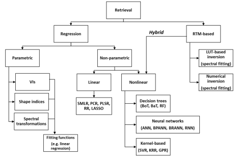
Figure 9: Schematic overview main retrieval methods.

While pros and cons of each of these methodological categories have been earlier discussed (Verrelst et al, 2015), here we discuss these categories from the perspective of forthcoming routinely-acquired and standardized (e.g., atmospherically-corrected) imaging spectroscopy data streams. First of all, the choice of a method bears implications; not only on the retrievability and processing time of mappable vegetation properties, but also on the purpose of the retrieval. Parametric and non-parametric methods rely on ground data for training, which obviously need to be available in order to apply these methods. If they are available, they are the ’shortest’ way to the variables of interest, because especially the non-parametric methods do no impose any limitation on the relationship between the spectrum and the variable of interest. In contrast, RTMs describe radiative transfer processes, i.e. they use existing knowledge (as materialized in the models) rather than ground measured data. Retrieval from an RTM through inversion is most useful if one is more interested in the underlying radiative transfer processes (scattering, sun- and shade foliage fractions, light distribution within vegetation canopies, relationships between canopy structure and photosynthesis), rather than in merely extracting a specific variable. However, strategies relying on RTM simulations are inherently limited by the input variables of the RTM and, as discussed in section 4, ancillary data and regularization methods may be required to optimize their inversions.

Statistical approaches, on the other hand, possess the flexibility to relate reflectance data with any measured biophysical variable – state variable or not. As has been demonstrated in sections 2 and 3, this can be any quantifiable attribute, typically in the domains of leaf biochemical constituents (e.g., nitrogen, phosphorus), pigments (e.g., chlorophyll, cartenoids, xanthophylls) or higher-level structural variables (e.g., above-ground biomass, grain yield). The strength of the correlation with validation data typically determines the validity and transferrability of the statistical model. While this ’seeking for best correlations’ can be criticized, because of the absence of a physical basis (Knyazikhin et al, 2013), statistical approaches are becoming increasingly powerful to extract biochemical variables through complex and often indirect relationships. Particularly, machine learning models are powerful in extracting information from subtle variations in spectroscopic data through adaptive, nonlinear relationships. The advantage of these statistical models is that not only variable-specific absorption features can be used for information extraction, but also secondary relationships with variables related to other absorption features that co-vary with the variable of interest can be exploited (Ollinger, 2011; Verrelst et al, 2012b). Since high accuracies are often obtained with these methods, they are gaining popularity, not only for quantification of a diversity of vegetation properties, but also in mapping of floristic composition (Roth et al, 2015; Harris et al, 2015; Neumann et al, 2016; Feilhauer et al, 2017).

Regardless of the nature of retrieval method, in view of mapping larger areas, and especially in an operational and global context, what matters is the possibility to provide associated information on the retrieval quality. The characterization of uncertainty is a fundamental requirement for postulating correct scientific conclusions from results and for assimilating results into statistical or mechanistic higher-level models (Cressie et al, 2009). As addressed in section 2, parametric regression methods, i.e. spectral transformation methods in combination with a fitting function, do not provide uncertainty estimates, which undermine their applicability to other images in space and time. Subsequently, while valid when locally calibrated and validated, parametric methods are of little use in an operational context. With regard to inversion routines, uncertainties can be provided as spectral residuals (Rivera et al, 2013) or standard deviations when mapping multiple solution means (Verrelst et al, 2014). Lately, inversion approaches were proposed in a Bayesian framework (Shiklomanov et al, 2016), whereby uncertainties are delivered along with the retrievals. In case of traditional statistical models, uncertainty estimation has been a complex exercise. Statistical models developed within a Bayesian framework, such as GPR, provide uncertainties together with the predictions (Verrelst et al, 2013b; Camps-Valls et al, 2016), which indicate the probability interval of an estimation relative to the samples used during the training phase. These uncertainties can be used to evaluate GPR model transferability. For example, by mapping the uncertainties (Verrelst et al, 2013b) demonstrated that a locally developed regression model can be successfully transported to other images in space and time for the large majority of pixels (i.e., the uncertainty maps were not systematically worse). Similarly, uncertainties can inform about the model performance. It was demonstrated that dimensionality reduction methods applied in GPR models for LAI mapping not only largely sped up the processing, but they also led to lower per-pixel uncertainties as opposed to mapping using all bands (Rivera-Caicedo et al, 2017). In conclusion, in the view of an operational processing need, just as important as the variable retrieval itself is the provision of an associated uncertainty estimate. Uncertainty estimates allow evaluating the method’s per-pixel performance, and consequently allow evaluating the method’s capability to process routinely acquired imaging data. They thus provide a measure of the retrieval fidelity, which can be used to identify and mask out the highly uncertain and non-reliable results.

Another important aspect for operational production of vegetation properties from typically bulky imaging spectroscopy data streams implies computational speed. Generally, the lower the complexity of a model the faster it will be able to produce maps. This highly favors the application of parametric regression approaches since they consist of only few transformations and equations. Also non-parametric regression algorithms, once trained, can be applied to process an images almost instantaneously. Training of machine learning models is frequently related to the tuning of several free variables with costly cross-validation approaches. These scale poorly with the number of samples (such as in kernel machines) or with the data dimensions (such as in ANNs). Although a trained ANN converts an image into a map quasi-instantly, kernel-based methods require more processing time, because the similarity between each test pixel in the image and those used to train the model has to be estimated. Training can be computationally costly, especially when using a big training dataset, e.g. as in hybrid strategies. A solution to shorten training time could be in size reduction of the training data in a way that maximal relevant information is preserved. This can be achieved by means of dimensionality reduction methods in the spectral domain (Rivera-Caicedo et al, 2017), or by means of intelligent sampling in the sampling domain, e.g. through active learning (Verrelst et al, 2016a).

Considerably longer run-time is expected in case of inversion routines. Since RTMs take some time to generate simulations, especially for computationally expensive models, and also the evaluation takes place on a per-pixel basis, the iterative inversion routines are computationally expensive leading to relatively slow mapping speeds. In an attempt to accelerate their mapping speed, it has been proposed to approximate the functioning of the original RTM by means of statistical learning called emulation (Gómez-Dans et al, 2016; Rivera et al, 2015). Initial experiments to emulate leaf, canopy and atmospheric RTMs demonstrated that emulators can successfully generate spectral output from a limited set of input variable almost instantly, thereby preserving sufficient accuracy as compared to the original RTM (Verrelst et al, 2016c, 2017). Although an emulator reproduces RTM simulations instantly, application of a per-pixel spectral fitting requires many repetitions, which implies that these methods still do not reach the speed of statistical methods.

All in all, having the purpose of advancing towards operational imaging spectroscopy data processing in mind, i.e., reaching globally-applicable, accurate and fast estimates, we end up with the following recommendations:

• To enable model transferability to routinely-acquired images, retrieval methods must provide associated per-pixel uncertainties as a quality indicator whether the model can perform adequately in another space and time.

• Regarding the computational speed, e.g. in case of repetitive image processing, statistical (i.e. regression) methods are multiple times faster than physically-based methods, capable to process full images in the order of minutes or even seconds.

• In case of regression methods (experimental or hybrid), multicollinearity of spectroscopic data complicates the development of powerful models. Physically-based methods using spectral fitting do not suffer from this problem.

• To mitigate the problem of multicollinearity in regression methods, either band selection or dimensionality reduction methods can be applied before entering the regression. Although band selection is a common practice, likely more powerful regression models can be obtained when using a dimensionality reduction method.

7 Conclusions

With forthcoming imaging spectrometer satellite missions, an unprecedented stream of datasets on the terrestrial biosphere will become available. This will require powerful processing techniques enabling quantification of vegetation variables in an operational and global setting. Four categories of retrieval methods have been discussed in this review paper: (1) parametric regression; (2) non-parametric regression; (3) physically-based RTM inversion; and, (4) hybrid methods. For each of these categories, a diversity of methodological approaches are increasingly applied to imaging spectroscopy data. This literature review synthesized the current state-of-the-art in the field of spectroscopy-based vegetation properties mapping.

Although parametric methods, such as shape indices or spectral transformation, deal well with extracting relevant information embedded in spectroscopic data, their lack of uncertainty estimates makes them unsuitable for operational use. Higher accuracies can be reached with nonlinear non-parametric methods; especially those in the field of machine learning that generate probabilistic outputs, e.g. Gaussian process regression. However, an additional step to mitigate their spectral multicollinearity is deemed necessary. A popular strategy in this respect is selecting a set of vegetation indices or applying spectral transformation before training the machine learning algorithm. It remains nevertheless questionable whether such band selection approaches fully capture all relevant information. Instead, dimensionality reduction methods that enable compressing the large majority of spectral variability into a few components tend to lead to more accurate predictions.

On the other hand, the inversion of physically-based RTMs against spectroscopic data is generally applicable and physically sound, but optimizing their inversion strategies is more challenging compared to the regression methods. RTM-based inversion is computationally demanding and ancillary information is usually required as an input or to regulate the inversion algorithm. Hybrid regression methods, based on the coupling of an RTM with a machine learning regression algorithm, overcome the problem of processing speed. Particularly Bayesian kernel-based hybrid strategies possess promising features, as they combine speed, flexibility and the provision of uncertainty estimates. Their accuracies and processing speed can be further improved in combination with dimensionality reduction. Altogether, and in the interest of operational spectroscopy-based mapping of vegetation properties, we recommend to further explore the feasibility and implementation of hybrid strategies into the next-generation data processing chains.

References

- Adam et al (2014) Adam E, Mutanga O, Abdel-Rahman E, Ismail R (2014) Estimating standing biomass in papyrus (Cyperus papyrus L.) swamp: Exploratory of in situ hyperspectral indices and random forest regression. International Journal of Remote Sensing 35(2):693–714
- Addink et al (2007) Addink E, De Jong S, Pebesma E (2007) The importance of scale in object-based mapping of vegetation parameters with hyperspectral imagery. Photogrammetric Engineering and Remote Sensing 73(8):905–912
- Ali et al (2016) Ali A, Skidmore A, Darvishzadeh R, van Duren I, Holzwarth S, Mueller J (2016) Retrieval of forest leaf functional traits from HySpex imagery using radiative transfer models and continuous wavelet analysis. ISPRS Journal of Photogrammetry and Remote Sensing 122:68–80
- Alton et al (2007) Alton P, Ellis R, Los S, North P (2007) Improved global simulations of gross primary product based on a separate and explicit treatment of diffuse and direct sunlight. Journal of Geophysical Research: Atmospheres 112(D7)
- Arellano et al (2017) Arellano P, Tansey K, Balzter H, Tellkamp M (2017) Plant family-specific impacts of petroleum pollution on biodiversity and leaf chlorophyll content in the Amazon rainforest of Ecuador. PLoS ONE 12(1)
- Arenas-García and Camps-Valls (2008) Arenas-García J, Camps-Valls G (2008) Efficient kernel orthonormalized PLS for remote sensing applications. IEEE Transactions on Geoscience and Remote Sensing 46(10):2872–2881
- Ashourloo et al (2016) Ashourloo D, Aghighi H, Matkan A, Mobasheri M, Rad A (2016) An investigation into machine learning regression techniques for the leaf rust disease detection using hyperspectral measurement. IEEE Journal of Selected Topics in Applied Earth Observations and Remote Sensing 9(9):4344–4351
- Atzberger et al (2010) Atzberger C, Guérif M, Baret F, Werner W (2010) Comparative analysis of three chemometric techniques for the spectroradiometric assessment of canopy chlorophyll content in winter wheat. Computers and Electronics in Agriculture 73(2):165–173
- Atzberger et al (2015) Atzberger C, Darvishzadeh R, Immitzer M, Schlerf M, Skidmore A, le Maire G (2015) Comparative analysis of different retrieval methods for mapping grassland leaf area index using airborne imaging spectroscopy. International Journal of Applied Earth Observation and Geoinformation 43:19–31
- Bacour et al (2006) Bacour C, Baret F, Béal D, Weiss M, Pavageau K (2006) Neural network estimation of LAI, fAPAR, fCover and LAICab, from top of canopy MERIS reflectance data: Principles and validation. Remote Sensing of Environment 105(4):313–325
- Balzarolo et al (2015) Balzarolo M, Vescovo L, Hammerle A, Gianelle D, Papale D, Tomelleri E, Wohlfahrt G (2015) On the relationship between ecosystem-scale hyperspectral reflectance and exchange in European mountain grasslands. Biogeosciences 12(10):3089–3108
- Banskota et al (2013) Banskota A, Wynne R, Thomas V, Serbin S, Kayastha N, Gastellu-Etchegorry J, Townsend P (2013) Investigating the utility of wavelet transforms for inverting a 3-D radiative transfer model using hyperspectral data to retrieve forest LAI. Remote Sensing 5(6):2639–2659
- Banskota et al (2015) Banskota A, Serbin S, Wynne R, Thomas V, Falkowski M, Kayastha N, Gastellu-Etchegorry JP, Townsend P (2015) An LUT-Based Inversion of DART Model to Estimate Forest LAI from Hyperspectral Data. IEEE Journal of Selected Topics in Applied Earth Observations and Remote Sensing 8(6):3147–3160
- Bao et al (2017) Bao S, Cao C, Chen W, Tian H (2017) Spectral features and separability of alpine wetland grass species. Spectroscopy Letters 50(5):245–256
- Baranoski and Rokne (2005) Baranoski G, Rokne J (2005) A practical approach for estimating the red edge position of plant leaf reflectance. International Journal of Remote Sensing 26(3):503–521
- Baret and Buis (2008) Baret F, Buis S (2008) Estimating canopy characteristics from remote sensing observations. Review of methods and associated problems. In S Liang (Ed), Advances in Land Remote Sensing: System, Modeling, Inversion and Application, Springer pp 171–200
- Baret et al (2013) Baret F, Weiss M, Lacaze R, Camacho F, Makhmara H, Pacholcyzk P, Smets B (2013) GEOV1: LAI and FAPAR essential climate variables and FCOVER global time series capitalizing over existing products. Part1: Principles of development and production . Remote Sensing of Environment 137(0):299 – 309
- Barton and North (2001) Barton CVM, North P (2001) Remote sensing of canopy light use efficiency using the photochemical reflectance index: Model and sensitivity analysis. Remote Sensing of Environment 78(3):264–273
- Bayat et al (2016) Bayat B, van der Tol C, Verhoef W (2016) Remote sensing of grass response to drought stress using spectroscopic techniques and canopy reflectance model inversion. Remote Sensing 8(7)
- Belgiu and Drăguţ (2016) Belgiu M, Drăguţ L (2016) Random forest in remote sensing: A review of applications and future directions. ISPRS Journal of Photogrammetry and Remote Sensing 114:24–31
- Berk et al (2006) Berk A, Anderson G, Acharya P, Bernstein L, Muratov L, Lee J, Fox M, Adler-Golden S, Chetwynd J, Hoke M, Lockwood R, Gardner J, Cooley T, Borel C, Lewis P, Shettle E (2006) MODTRANTM5: 2006 update. vol 6233 II
- Botha et al (2007) Botha E, Leblon B, Zebarth B, Watmough J (2007) Non-destructive estimation of potato leaf chlorophyll from canopy hyperspectral reflectance using the inverted PROSAIL model. International Journal of Applied Earth Observation and Geoinformation 9(4):360–374
- Bratsch et al (2017) Bratsch S, Epstein H, Buchhorn M, Walker D, Landes H (2017) Relationships between hyperspectral data and components of vegetation biomass in Low Arctic tundra communities at Ivotuk, Alaska. Environmental Research Letters 12(2)
- Breiman (1996) Breiman L (1996) Bagging predictors. Machine Learning 24(2):123–140
- Breiman (2001) Breiman L (2001) Random forests. Machine Learning 45(1):5–32
- Breiman et al (1984) Breiman L, Friedman J, Stone C, Olshen R (1984) Classification and Regression Trees. The Wadsworth and Brooks-Cole statistics-probability series, Taylor & Francis
- Broge and Leblanc (2001) Broge NH, Leblanc E (2001) Comparing prediction power and stability of broadband and hyperspectral vegetation indices for estimation of green leaf area index and canopy chlorophyll density. Remote Sensing of Environment 76(2):156–172
- Broomhead and Lowe (1988) Broomhead DS, Lowe D (1988) Radial basis functions, multi-variable functional interpolation and adaptive networks. Tech. rep., Royal Signals and Radar Establishment Malvern (United Kingdom)
- Buchhorn et al (2013) Buchhorn M, Walker DA, Heim B, Raynolds MK, Epstein HE, Schwieder M (2013) Ground-based hyperspectral characterization of alaska tundra vegetation along environmental gradients. Remote Sensing 5(8):3971–4005
- Burden and Winkler (1999) Burden F, Winkler D (1999) Robust QSAR models using bayesian regularized neural networks. Journal of Medicinal Chemistry 42(16):3183–3187
- Bye et al (2017) Bye I, North P, Los S, Kljun N, Rosette J, Hopkinson C, Chasmer L, Mahoney C (2017) Estimating forest canopy parameters from satellite waveform LiDAR by inversion of the FLIGHT three-dimensional radiative transfer model. Remote Sensing of Environment 188:177–189
- Camps-Valls et al (2016) Camps-Valls G, Verrelst J, Muñoz-Marí J, Laparra V, Mateo-Jiménez F, Gómez-Dans J (2016) A survey on Gaussian processes for earth observation data analysis. IEEE Geoscience and Remote Sensing Magazine 4(2)
- Capolupo et al (2015) Capolupo A, Kooistra L, Berendonk C, Boccia L, Suomalainen J (2015) Estimating plant traits of grasslands from UAV-acquired hyperspectral images: A comparison of statistical approaches. ISPRS International Journal of Geo-Information 4(4):2792–2820
- Chen et al (2015) Chen B, Wu Z, Wang J, Dong J, Guan L, Chen J, Yang K, Xie G (2015) Spatio-temporal prediction of leaf area index of rubber plantation using HJ-1A/1B CCD images and recurrent neural network. ISPRS Journal of Photogrammetry and Remote Sensing 102:148–160
- Cho and Skidmore (2006) Cho MA, Skidmore AK (2006) A new technique for extracting the red edge position from hyperspectral data: The linear extrapolation method. Remote sensing of environment 101(2):181–193
- Cho et al (2008) Cho MA, Skidmore AK, Atzberger C (2008) Towards red-edge positions less sensitive to canopy biophysical parameters for leaf chlorophyll estimation using properties optique spectrales des feuilles (PROSPECT) and scattering by arbitrarily inclined leaves (SAILH) simulated data. International Journal of Remote Sensing 29(8):2241–2255
- Cho et al (2007) Cho Mb, Skidmore Ab, Corsi F, van Wieren S, Sobhan Ib (2007) Estimation of green grass/herb biomass from airborne hyperspectral imagery using spectral indices and partial least squares regression. International Journal of Applied Earth Observation and Geoinformation 9(4):414–424
- Clark and Roush (1984) Clark RN, Roush TL (1984) Reflectance spectroscopy: Quantitative analysis techniques for remote sensing applications. Journal of Geophysical Research: Solid Earth 89(B7):6329–6340
- Clevers (2014) Clevers J (2014) Beyond NDVI: Extraction of biophysical variables from remote sensing imagery. Remote Sensing and Digital Image Processing 18:363–381
- Clevers and Kooistra (2012) Clevers J, Kooistra L (2012) Using hyperspectral remote sensing data for retrieving canopy chlorophyll and nitrogen content. IEEE Journal of Selected Topics in Applied Earth Observations and Remote Sensing 5(2):574–583
- Clevers et al (2004) Clevers JGPW, Kooistra L, Salas EAL (2004) Study of heavy metal contamination in river floodplains using the red-edge position in spectroscopic data. International Journal of Remote Sensing 25(19):3883–3895
- Coops et al (2003) Coops NC, Smith ML, Martin M, Ollinger SV (2003) Prediction of eucalypt foliage nitrogen content from satellite-derived hyperspectral data. IEEE Transactions on Geoscience and Remote Sensing 41(6):1338–1346
- Cressie et al (2009) Cressie N, Calder C, Clark J, Ver Hoef J, Wikle C (2009) Accounting for uncertainty in ecological analysis: The strengths and limitations of hierarchical statistical modeling. Ecological Applications 19(3):553–570
- Danner et al (2017) Danner M, Berger K, Wocher M, Mauser W, Hank T (2017) Retrieval of biophysical crop variables from multi-angular canopy spectroscopy. Remote Sensing 9(7)
- Darvishzadeh et al (2008) Darvishzadeh R, Skidmore A, Schlerf M, Atzberger C (2008) Inversion of a radiative transfer model for estimating vegetation LAI and chlorophyll in a heterogeneous grassland. Remote Sensing of Environment 112(5):2592–2604
- Darvishzadeh et al (2012) Darvishzadeh R, Matkan AA, Dashti Ahangar A (2012) Inversion of a radiative transfer model for estimation of rice canopy chlorophyll content using a lookup-table approach. IEEE Journal of Selected Topics in Applied Earth Observations and Remote Sensing PP(99):1 –9
- Dawson et al (1998) Dawson T, Curran P, Plummer S (1998) LIBERTY - Modeling the effects of Leaf Biochemical Concentration on Reflectance Spectra. Remote Sensing of Environment 65(1):50–60
- Delegido et al (2010) Delegido J, Alonso L, González G, Moreno J (2010) Estimating chlorophyll content of crops from hyperspectral data using a normalized area over reflectance curve (NAOC). International Journal of Applied Earth Observation and Geoinformation 12(3):165–174
- Delegido et al (2011) Delegido J, Verrelst J, Alonso L, Moreno J (2011) Evaluation of sentinel-2 red-edge bands for empirical estimation of green LAI and chlorophyll content. Sensors 11(7):7063–7081
- Delegido et al (2013) Delegido J, Verrelst J, Meza C, Rivera J, Alonso L, Moreno J (2013) A red-edge spectral index for remote sensing estimation of green LAI over agroecosystems. European Journal of Agronomy 46:42–52
- Dietz et al (2012) Dietz A, Kuenzer C, Gessner U, Dech S (2012) Remote sensing of snow - a review of available methods. International Journal of Remote Sensing 33(13):4094–4134
- Disney et al (2006) Disney M, Lewis P, Saich P (2006) 3D modelling of forest canopy structure for remote sensing simulations in the optical and microwave domains. Remote Sensing of Environment 100(1):114–132
- Doktor et al (2014) Doktor D, Lausch A, Spengler D, Thurner M (2014) Extraction of plant physiological status from hyperspectral signatures using machine learning methods. Remote Sensing 6(12):12,247–12,274
- Dorigo et al (2009) Dorigo W, Richter R, Baret F, Bamler R, Wagner W (2009) Enhanced automated canopy characterization from hyperspectral data by a novel two step radiative transfer model inversion approach. Remote Sensing 1(4):1139–1170
- Dorigo et al (2007) Dorigo WA, Zurita-Milla R, de Wit AJW, Brazile J, Singh R, Schaepman ME (2007) A review on reflective remote sensing and data assimilation techniques for enhanced agroecosystem modeling. International Journal of Applied Earth Observation and Geoinformation 9(2):165–193
- Draper and Smith (2014) Draper NR, Smith H (2014) Applied regression analysis. John Wiley & Sons
- Dreccer et al (2014) Dreccer M, Barnes L, Meder R (2014) Quantitative dynamics of stem water soluble carbohydrates in wheat can be monitored in the field using hyperspectral reflectance. Field Crops Research 159:70–80
- Drusch et al (2017) Drusch M, Moreno J, Del Bello U, Franco R, Goulas Y, Huth A, Kraft S, Middleton EM, Miglietta F, Mohammed G, et al (2017) The FLuorescence EXplorer Mission Concept-ESA’s Earth Explorer 8. IEEE Transactions on Geoscience and Remote Sensing 55(3):1273–1284
- Du et al (2016) Du L, Shi S, Yang J, Sun J, Gong W (2016) Using different regression methods to estimate leaf nitrogen content in rice by fusing hyperspectral LiDAR data and laser-induced chlorophyll fluorescence data. Remote Sensing 8(6)
- Duan et al (2014) Duan SB, Li ZL, Wu H, Tang BH, Ma L, Zhao E, Li C (2014) Inversion of the prosail model to estimate leaf area index of maize, potato, and sunflower fields from unmanned aerial vehicle hyperspectral data. International Journal of Applied Earth Observation and Geoinformation 26(1):12–20
- Elvidge and Chen (1995) Elvidge CD, Chen Z (1995) Comparison of broad-band and narrow-band red and near-infrared vegetation indices. Remote Sensing of Environment 54(1):38–48
- Favennec et al (2016) Favennec Y, Le Hardy D, Dubot F, Rousseau B, Rousse D (2016) Some speed-up strategies for solving inverse radiative transfer problems. Journal of Physics: Conference Series 676(1)
- Fei et al (2012) Fei Y, Jiulin S, Hongliang F, Zuofang Y, Jiahua Z, Yunqiang Z, Kaishan S, Zongming W, Maogui H (2012) Comparison of different methods for corn LAI estimation over northeastern China. International Journal of Applied Earth Observation and Geoinformation 18:462–471
- Feilhauer et al (2015) Feilhauer H, Asner GP, Martin RE (2015) Multi-method ensemble selection of spectral bands related to leaf biochemistry. Remote Sensing of Environment 164:57 – 65
- Feilhauer et al (2017) Feilhauer H, Somers B, van der Linden S (2017) Optical trait indicators for remote sensing of plant species composition: Predictive power and seasonal variability. Ecological Indicators 73:825–833
- Feng et al (2016) Feng H, Yang F, Li Z, Yang G, Guo J, He P, Wang Y (2016) Hyperspectral estimation of leaf total phosphorus content in apple tree based on optimal weights combination model. Nongye Gongcheng Xuebao/Transactions of the Chinese Society of Agricultural Engineering 32(7):173–180
- Feret et al (2008) Feret JB, François C, Asner GP, Gitelson AA, Martin RE, Bidel LPR, Ustin SL, le Maire G, Jacquemoud S (2008) PROSPECT-4 and 5: Advances in the leaf optical properties model separating photosynthetic pigments. Remote Sensing of Environment 112(6):3030–3043
- Foster et al (2017) Foster A, Kakani V, Mosali J (2017) Estimation of bioenergy crop yield and N status by hyperspectral canopy reflectance and partial least square regression. Precision Agriculture 18(2):192–209
- Francl and Panigrahi (1997) Francl L, Panigrahi S (1997) Artificial neural network models of wheat leaf wetness. Agricultural and Forest Meteorology 88(1-4):57–65
- Friedman et al (2000) Friedman J, Hastie T, Tibshirani R (2000) Additive logistic regression: A statistical view of boosting. Annals of Statistics 28(2):337–407
- Fu et al (2012) Fu Y, Yang G, Feng H, Xu X, Song X, Wang J (2012) Comparison of winter wheat LAI estimation methods based on hyperspectral dimensionality reduction and vegetation index. Nongye Gongcheng Xuebao/Transactions of the Chinese Society of Agricultural Engineering 28(23):107–113
- Gastellu-Etchegorry et al (1996) Gastellu-Etchegorry J, Demarez V, Pinel V, Zagolski F (1996) Modeling radiative transfer in heterogeneous 3-D vegetation canopies. Remote Sensing of Environment 58(2):131–156
- Gastellu-Etchegorry et al (1999) Gastellu-Etchegorry J, Guillevic P, Zagolski F, Demarez V, Trichon V, Deering D, Leroy M (1999) Modeling BRF and radiation regime of boreal and tropical forests: I. BRF. Remote Sensing of Environment 68(3):281–316
- Gastellu-Etchegorry et al (2003) Gastellu-Etchegorry J, Gascon F, Esteve P (2003) An interpolation procedure for generalizing a look-up table inversion method. Remote Sensing of Environment 87(1):55–71
- Gastellu-Etchegorry et al (2004) Gastellu-Etchegorry J, Martin E, Gascon F (2004) DART: a 3D model for simulating satellite images and studying surface radiation budget. International journal of remote sensing 25(1):73–96
- Gastellu-Etchegorry et al (2017) Gastellu-Etchegorry J, Lauret N, Yin T, Landier L, Kallel A, Malenovský Z, Al Bitar A, Aval J, Benhmida S, Qi J, Medjdoub G, Guilleux J, Chavanon E, Cook B, Morton D, Nektarios N, Mitraka Z (2017) DART: Recent advances in remote sensing data modeling with atmosphere, polarization, and chlorophyll fluorescence. IEEE Journal of Selected Topics in Applied Earth Observations and Remote Sensing p In press (accepted 8 March 2017)
- Gastellu-Etchegorry et al (2015) Gastellu-Etchegorry JP, Yin T, Lauret N, Cajgfinger T, Gregoire T, Grau E, Feret JB, Lopes M, Guilleux J, Dedieu G, Malenovský Z, Cook B, Morton D, Rubio J, Durrieu S, Cazanave G, Martin E, Ristorcelli T (2015) Discrete anisotropic radiative transfer (DART 5) for modeling airborne and satellite spectroradiometer and LIDAR acquisitions of natural and urban landscapes. Remote Sensing 7(2):1667–1701
- Gastellu-Etchegorry et al (2016) Gastellu-Etchegorry JP, Yin T, Lauret N, Grau E, Rubio J, Cook B, Morton D, Sun G (2016) Simulation of satellite, airborne and terrestrial LiDAR with DART (I): Waveform simulation with quasi-Monte Carlo ray tracing. Remote Sensing of Environment 184:418–435
- Geladi and Kowalski (1986) Geladi P, Kowalski B (1986) Partial least-squares regression: a tutorial. Analytica Chimica Acta 185(C):1–17
- Gewali et al (2018) Gewali U, Monteiro S, Saber E (2018) Machine learning based hyperspectral image analysis: A survey. ISPRS Journal of Photogrammetry and Remote Sensing (submitted)
- Gianelle and Guastella (2007) Gianelle D, Guastella Fb (2007) Nadir and off-nadir hyperspectral field data: Strengths and limitations in estimating grassland biophysical characteristics. International Journal of Remote Sensing 28(7):1547–1560
- Glenn et al (2008) Glenn E, Huete A, Nagler P, Nelson S (2008) Relationship between remotely-sensed vegetation indices, canopy attributes and plant physiological processes: What vegetation indices can and cannot tell us about the landscape. Sensors 8(4):2136–2160
- Gómez-Chova et al (2011) Gómez-Chova L, Muñoz-Marí J, Laparra V, Malo-López J, Camps-Valls G (2011) A review of kernel methods in remote sensing data analysis. In: Optical Remote Sensing, Springer, pp 171–206
- Gómez-Dans et al (2016) Gómez-Dans JL, Lewis PE, Disney M (2016) Efficient emulation of radiative transfer codes using gaussian processes and application to land surface parameter inferences. Remote Sensing 8(2):119
- Gonsamo (2011) Gonsamo A (2011) Normalized sensitivity measures for leaf area index estimation using three-band spectral vegetation indices. International Journal of Remote Sensing 32(7):2069–2080
- Govaerts and Verstraete (1998) Govaerts YM, Verstraete MM (1998) Raytran: A Monte Carlo ray-tracing model to compute light scattering in three-dimensional heterogeneous media. IEEE Transactions on Geoscience and Remote Sensing 36(2):493–505
- Grau and Gastellu-Etchegorry (2013) Grau E, Gastellu-Etchegorry JP (2013) Radiative transfer modeling in the Earth–Atmosphere system with DART model. Remote sensing of environment 139:149–170
- Guanter et al (2015) Guanter L, Kaufmann H, Segl K, Foerster S, Rogass C, Chabrillat S, Kuester T, Hollstein A, Rossner G, Chlebek C, Straif C, Fischer S, Schrader S, Storch T, Heiden U, Mueller A, Bachmann M, Muhle H, Muller R, Habermeyer M, Ohndorf A, Hill J, Buddenbaum H, Hostert P, van der Linden S, Leitao PJ, Rabe A, Doerffer R, Krasemann H, Xi H, Mauser W, Hank T, Locherer M, Rast M, Staenz K, Sang B (2015) The EnMAP Spaceborne Imaging Spectroscopy Mission for Earth Observation. Remote Sensing 7(7):8830
- Guillevic et al (2003) Guillevic P, Gastellu-Etchegorry J, Demarty J, Prévot L (2003) Thermal infrared radiative transfer within three-dimensional vegetation covers. Journal of Geophysical Research: Atmospheres 108(D8)
- Han et al (2016) Han ZY, Zhu XC, Fang XY, Wang ZY, Wang L, Zhao GX, Jiang YM (2016) Hyperspectral estimation of apple tree canopy LAI based on SVM and RF regression. Guang Pu Xue Yu Guang Pu Fen Xi/Spectroscopy and Spectral Analysis 36(3):800–805
- Hancock et al (2012) Hancock S, Lewis P, Foster M, Disney M, Muller JP (2012) Measuring forests with dual wavelength lidar: A simulation study over topography. Agricultural and Forest Meteorology 161:123–133
- Hansen and Schjoerring (2003) Hansen PM, Schjoerring JK (2003) Reflectance measurement of canopy biomass and nitrogen status in wheat crops using normalized difference vegetation indices and partial least squares regression. Remote Sensing of Environment 86(4):542–553
- Harris et al (2015) Harris A, Charnock R, Lucas R (2015) Hyperspectral remote sensing of peatland floristic gradients. Remote Sensing of Environment 162:99–111
- Haykin (1999) Haykin S (1999) Neural Networks – A Comprehensive Foundation, 2nd edn. Prentice Hall
- He et al (2015) He R, Qiao X, Jiang J, Guo H (2015) Retrieving canopy leaf total nitrogen content of winter wheat by continuous wavelet transform. Nongye Gongcheng Xuebao/Transactions of the Chinese Society of Agricultural Engineering 31(2):141–146
- Heiskanen et al (2013) Heiskanen J, Rautiainen M, Stenberg P, Mõttus M, Vesanto VH (2013) Sensitivity of narrowband vegetation indices to boreal forest LAI, reflectance seasonality and species composition. ISPRS Journal of Photogrammetry and Remote Sensing 78:1–14
- Hernández-Clemente et al (2017) Hernández-Clemente R, North P, Hornero A, Zarco-Tejada P (2017) Assessing the effects of forest health on sun-induced chlorophyll fluorescence using the FluorFLIGHT 3-D radiative transfer model to account for forest structure. Remote Sensing of Environment 193:165–179
- Hochreiter and Schmidhuber (1997) Hochreiter S, Schmidhuber J (1997) Long short-term memory. Neural Computation 9(8):1735–1780
- Homolová et al (2016) Homolová L, Janoutová R, Malenovský Z (2016) Evaluation of various spectral inputs for estimation of forest biochemical and structural properties from airborne imaging spectroscopy data. vol 41, pp 961–966
- Huang et al (2014) Huang Y, Tian Q, Wang L, Geng J, Lyu C (2014) Estimating canopy leaf area index in the late stages of wheat growth using continuous wavelet transform. Journal of Applied Remote Sensing 8(1)
- Huang et al (2004) Huang Z, Turner BJ, Dury SJ, Wallis IR, Foley WJ (2004) Estimating foliage nitrogen concentration from HYMAP data using continuum removal analysis. Remote Sensing of Environment 93(1):18–29
- Hughes (1968) Hughes G (1968) On the mean accuracy of statistical pattern recognizers. IEEE Transactions on Information Theory 14(1):55–63
- Im et al (2009) Im J, Jensen JR, Coleman M, Nelson E (2009) Hyperspectral remote sensing analysis of short rotation woody crops grown with controlled nutrient and irrigation treatments. Geocarto International 24(4):293–312
- Jacquemoud et al (1995) Jacquemoud S, Baret F, Andrieu B, Danson FM, Jaggard K (1995) Extraction of vegetation biophysical parameters by inversion of the PROSPECT+SAIL models on sugar beet canopy reflectance data. Application to TM and AVIRIS sensors. Remote Sensing of Environment 52(3):163–172
- Jacquemoud et al (2009a) Jacquemoud S, Verhoef W, Baret F, Bacour C, Zarco-Tejada P, Asner G, François C, Ustin S (2009a) PROSPECT + SAIL models: A review of use for vegetation characterization. Remote Sensing of Environment 113(SUPPL. 1):S56–S66
- Jacquemoud et al (2009b) Jacquemoud S, Verhoef W, Baret F, Bacour C, Zarco-Tejada P, Asner G, François C, Ustin S (2009b) PROSPECT + SAIL models: A review of use for vegetation characterization. Remote Sensing of Environment 113(SUPPL. 1):S56–S66
- Jay et al (2016) Jay S, Bendoula R, Hadoux X, Féret JB, Gorretta N (2016) A physically-based model for retrieving foliar biochemistry and leaf orientation using close-range imaging spectroscopy. Remote Sensing of Environment 177:220–236
- Jensen et al (2012) Jensen R, Hardin P, Hardin A (2012) Estimating urban leaf area index (LAI) of individual trees with hyperspectral data. Photogrammetric Engineering and Remote Sensing 78(5):495–504
- Jia et al (2013) Jia F, Liu G, Liu D, Zhang Y, Fan W, Xing X (2013) Comparison of different methods for estimating nitrogen concentration in flue-cured tobacco leaves based on hyperspectral reflectance. Field Crops Research 150:108–114
- Kalacska et al (2015) Kalacska M, Lalonde M, Moore T (2015) Estimation of foliar chlorophyll and nitrogen content in an ombrotrophic bog from hyperspectral data: Scaling from leaf to image. Remote Sensing of Environment 169:270–279
- Kanke et al (2016) Kanke Y, Tubaña B, Dalen M, Harrell D (2016) Evaluation of red and red-edge reflectance-based vegetation indices for rice biomass and grain yield prediction models in paddy fields. Precision Agriculture 17(5):507–530
- Karimi et al (2008) Karimi Y, Prasher S, Madani A, Kim S (2008) Application of support vector machine technology for the estimation of crop biophysical parameters using aerial hyperspectral observations. Canadian Biosystems Engineering / Le Genie des biosystems au Canada 50:7.13–7.20
- Kattenborn et al (2017) Kattenborn T, Fassnacht F, Pierce S, Lopatin J, Grime J, Schmidtlein S (2017) Linking plant strategies and plant traits derived by radiative transfer modelling. Journal of Vegetation Science 28(4):717–727
- Kempeneers et al (2008) Kempeneers P, Zarco-Tejada PJ, North PRJ, de Backer S, Delalieux S, Sepulcre-Cantó G, Morales F, van Aardt JAN, Sagardoy R, Coppin P, Scheunders P (2008) Model inversion for chlorophyll estimation in open canopies from hyperspectral imagery. International Journal of Remote Sensing 29(17-18):5093–5111
- Kiala et al (2016) Kiala Z, Odindi J, Mutanga O, Peerbhay K (2016) Comparison of partial least squares and support vector regressions for predicting leaf area index on a tropical grassland using hyperspectral data. Journal of Applied Remote Sensing 10(3)
- Kimes et al (1998) Kimes DS, Nelson RF, Manry MT, Fung AK (1998) Attributes of neural networks for extracting continuous vegetation variables from optical and radar measurements. International Journal of Remote Sensing 19(14):2639–2662
- Kira et al (2016) Kira O, Nguy-Robertson A, Arkebauer T, Linker R, Gitelson A (2016) Informative spectral bands for remote green LAI estimation in C3 and C4 crops. Agricultural and Forest Meteorology 218-219:243–249
- Knox et al (2011) Knox N, Skidmore A, Prins H, Asner G, van der Werff H, de Boer W, van der Waal C, de Knegt H, Kohi E, Slotow R, Grant R (2011) Dry season mapping of savanna forage quality, using the hyperspectral carnegie airborne observatory sensor. Remote Sensing of Environment 115(6):1478–1488
- Knyazikhin et al (2013) Knyazikhin Y, Schull MA, Stenberg P, Mõttus M, Rautiainen M, Yang Y, Marshak A, Carmona PL, Kaufmann RK, Lewis P, et al (2013) Hyperspectral remote sensing of foliar nitrogen content. Proceedings of the National Academy of Sciences 110(3):E185–E192
- Koetz et al (2005) Koetz B, Baret F, Poilvé H, Hill J (2005) Use of coupled canopy structure dynamic and radiative transfer models to estimate biophysical canopy characteristics. Remote Sensing of Environment 95(1):115–124
- Kováč et al (2013) Kováč D, Malenovský Z, Urban O, Špunda V, Kalina J, Ač A, Kaplan V, Hanuš J (2013) Response of green reflectance continuum removal index to the xanthophyll de-epoxidation cycle in norway spruce needles. Journal of experimental botany 64(7):1817–1827
- Labate et al (2009) Labate D, Ceccherini M, Cisbani A, De Cosmo V, Galeazzi C, Giunti L, Melozzi M, Pieraccini S, Stagi M (2009) The PRISMA payload optomechanical design, a high performance instrument for a new hyperspectral mission. Acta Astronautica 65(9-10):1429–1436
- Laurent et al (2013) Laurent V, Verhoef W, Damm A, Schaepman M, Clevers J (2013) A Bayesian object-based approach for estimating vegetation biophysical and biochemical variables from APEX at-sensor radiance data. Remote Sensing of Environment 139:6–17
- Laurent et al (2014) Laurent V, Schaepman M, Verhoef W, Weyermann J, Chávez R (2014) Bayesian object-based estimation of LAI and chlorophyll from a simulated Sentinel-2 top-of-atmosphere radiance image. Remote Sensing of Environment 140:318–329
- Lazaridis et al (2010) Lazaridis DC, Verbesselt J, Robinson AP (2010) Penalized regression techniques for prediction: a case study for predicting tree mortality using remotely sensed vegetation indices. Canadian journal of forest research 41(1):24–34
- Lazaro-Gredilla et al (2014) Lazaro-Gredilla M, Titsias M, Verrelst J, Camps-Valls G (2014) Retrieval of biophysical parameters with heteroscedastic Gaussian processes. IEEE Geoscience and Remote Sensing Letters 11(4):838–842
- Lee et al (2015) Lee CM, Cable ML, Hook SJ, Green RO, Ustin SL, Mandl DJ, Middleton EM (2015) An introduction to the nasa hyperspectral infrared imager (hyspiri) mission and preparatory activities. Remote Sensing of Environment 167:6 – 19, DOI https://doi.org/10.1016/j.rse.2015.06.012, special Issue on the Hyperspectral Infrared Imager (HyspIRI)
- Leonenko et al (2013) Leonenko G, North P, Los S (2013) Statistical distances and their applications to biophysical parameter estimation: Information measures, M-estimates, and minimum contrast methods. Remote Sensing 5(3):1355–1388
- Lewis (1999) Lewis P (1999) Three-dimensional plant modelling for remote sensing simulation studies using the botanical plant modelling system. Agronomie 19(3-4):185–210
- Lewis and Muller (1990) Lewis P, Muller J (1990) Botanical plant modelling for remote sensing simulation studies. In: Geoscience and Remote Sensing Symposium, 1990. IGARSS’90.’Remote Sensing Science for the Nineties’., 10th Annual International, IEEE, pp 1739–1742
- Lewis and Muller (1993) Lewis P, Muller J (1993) The advanced radiometric ray tracer: Ararat for plant canopy reflectance simulation. International Archives of Photogrammetry and Remote Sensing 29:26–26
- Li et al (2017) Li D, Cheng T, Zhou K, Zheng H, Yao X, Tian Y, Zhu Y, Cao W (2017) WREP: A wavelet-based technique for extracting the red edge position from reflectance spectra for estimating leaf and canopy chlorophyll contents of cereal crops. ISPRS Journal of Photogrammetry and Remote Sensing 129:103–117
- Li et al (2014a) Li L, Zhang Q, Huang D (2014a) A review of imaging techniques for plant phenotyping. Sensors (Switzerland) 14(11):20,078–20,111
- Li et al (2014b) Li X, Liu X, Liu M, Wu L (2014b) Random forest algorithm and regional applications of spectral inversion model for estimating canopy nitrogen concentration in rice. Yaogan Xuebao/Journal of Remote Sensing 18(4):934–945
- Liang et al (2015) Liang L, Di L, Zhang L, Deng M, Qin Z, Zhao S, Lin H (2015) Estimation of crop LAI using hyperspectral vegetation indices and a hybrid inversion method. Remote Sensing of Environment 165:123–134
- Liang et al (2016) Liang L, Qin Z, Zhao S, Di L, Zhang C, Deng M, Lin H, Zhang L, Wang L, Liu Z (2016) Estimating crop chlorophyll content with hyperspectral vegetation indices and the hybrid inversion method. International Journal of Remote Sensing 37(13):2923–2949
- Lin et al (2013) Lin H, Liang L, Zhang L, Du P (2013) Wheat leaf area index inversion with hyperspectral remote sensing based on support vector regression algorithm. Nongye Gongcheng Xuebao/Transactions of the Chinese Society of Agricultural Engineering 29(11):139–146
- Liu and Pan (2017) Liu WY, Pan J (2017) A hyperspectral assessment model for leaf chlorophyll content of Pinus massoniana based on neural network. Chinese Journal of Applied Ecology 28(4):1128–1136
- Locherer et al (2015) Locherer M, Hank T, Danner M, Mauser W (2015) Retrieval of seasonal leaf area index from simulated EnMAP data through optimized LUT-based inversion of the PROSAIL model. Remote Sensing 7(8):10,321–10,346
- Luo et al (2013) Luo J, Huang W, Zhao J, Zhang J, Zhao C, Ma R (2013) Detecting aphid density of winter wheat leaf using hyperspectral measurements. IEEE Journal of Selected Topics in Applied Earth Observations and Remote Sensing 6(2):690–698
- le Maire et al (2004) le Maire G, François C, Dufrene E (2004) Towards universal broad leaf chlorophyll indices using PROSPECT simulated database and hyperspectral reflectance measurements. Remote Sensing of Environment 89(1):1–28
- le Maire et al (2008) le Maire G, François C, Soudani K, Berveiller D, Pontailler JY, Bréda N, Genet H, Davi H, Dufrêne E (2008) Calibration and validation of hyperspectral indices for the estimation of broadleaved forest leaf chlorophyll content, leaf mass per area, leaf area index and leaf canopy biomass. Remote Sensing of Environment 112(10):3846–3864
- Malenovský et al (2006) Malenovský Z, Ufer C, Lhotakova Z, Clevers J, Schaepman M, Albrechtova J, Cudlin P (2006) A new hyperspectral index for chlorophyll estimation of a forest canopy: Area under curve normalised to maximal band depth between 650-725 nm. EARSeL EProceedings 5(2):161–172, cited By 25
- Malenovský et al (2013) Malenovský Z, Homolová L, Zurita-Milla R, Lukeš P, Kaplan V, Hanuš J, Gastellu-Etchegorry JP, Schaepman ME (2013) Retrieval of spruce leaf chlorophyll content from airborne image data using continuum removal and radiative transfer. Remote Sensing of Environment 131:85–102
- Malenovský et al (2015) Malenovský Z, Turnbull JD, Lucieer A, Robinson SA (2015) Antarctic moss stress assessment based on chlorophyll content and leaf density retrieved from imaging spectroscopy data. New Phytologist 208(2):608–624
- Malenovský et al (2017) Malenovský Z, Lucieer A, King D, Turnbull J, Robinson S (2017) Unmanned aircraft system advances health mapping of fragile polar vegetation. Methods in Ecology and Evolution
- Marabel and Alvarez-Taboada (2013) Marabel M, Alvarez-Taboada F (2013) Spectroscopic determination of aboveground biomass in grasslands using spectral transformations, support vector machine and partial least squares regression. Sensors (Switzerland) 13(8):10,027–10,051
- Mariotto et al (2013) Mariotto I, Thenkabail P, Huete A, Slonecker E, Platonov A (2013) Hyperspectral versus multispectral crop-productivity modeling and type discrimination for the HyspIRI mission. Remote Sensing of Environment 139:291–305
- Marshall and Thenkabail (2014) Marshall M, Thenkabail P (2014) Biomass modeling of four leading world crops using hyperspectral narrowbands in support of HyspIRI mission. Photogrammetric Engineering and Remote Sensing 80(8):757–772
- Matthes et al (2015) Matthes J, Knox S, Sturtevant C, Sonnentag O, Verfaillie J, Baldocchi D (2015) Predicting landscape-scale CO2 flux at a pasture and rice paddy with long-term hyperspectral canopy reflectance measurements. Biogeosciences 12(15):4577–4594
- Matthews (2011) Matthews M (2011) A current review of empirical procedures of remote sensing in inland and near-coastal transitional waters. International Journal of Remote Sensing 32(21):6855–6899
- Meroni et al (2004) Meroni M, Colombo R, Panigada C (2004) Inversion of a radiative transfer model with hyperspectral observations for LAI mapping in poplar plantations. Remote Sensing of Environment 92(2):195–206
- Miller et al (1990) Miller J, Hare E, Wu J (1990) Quantitative characterization of the vegetation red edge reflectance 1. An inverted-Gaussian reflectance model. Remote Sensing 11(10):1755–1773
- Miphokasap et al (2012) Miphokasap P, Honda K, Vaiphasa C, Souris M, Nagai M (2012) Estimating canopy nitrogen concentration in sugarcane using field imaging spectroscopy. Remote Sensing 4(6):1651–1670
- Mitchell et al (2012) Mitchell JJ, Glenn NF, Sankey TT, Derryberry DR, Germino MJ (2012) Remote sensing of sagebrush canopy nitrogen. Remote sensing of environment 124:217–223
- Montesano et al (2015) Montesano P, Rosette J, Sun G, North P, Nelson R, Dubayah R, Ranson K, Kharuk V (2015) The uncertainty of biomass estimates from modeled ICESat-2 returns across a boreal forest gradient. Remote Sensing of Environment 158:95–109
- Morton et al (2014) Morton DC, Nagol J, Carabajal CC, Rosette J, Palace M, Cook BD, Vermote EF, Harding DJ, North PR (2014) Amazon forests maintain consistent canopy structure and greenness during the dry season. Nature 506(7487):221–224
- Mulder et al (2011) Mulder V, de Bruin S, Schaepman M, Mayr T (2011) The use of remote sensing in soil and terrain mapping - a review. Geoderma 162(1-2):1–19
- Mutanga and Kumar (2007) Mutanga O, Kumar L (2007) Estimating and mapping grass phosphorus concentration in an African savanna using hyperspectral image data. International Journal of Remote Sensing 28(21):4897–4911
- Mutanga and Skidmore (2004) Mutanga O, Skidmore AK (2004) Narrow band vegetation indices overcome the saturation problem in biomass estimation. International Journal of Remote Sensing 25(19):3999–4014
- Mutanga et al (2005) Mutanga O, Skidmore AK, Kumar L, Ferwerda J (2005) Estimating tropical pasture quality at canopy level using band depth analysis with continuum removal in the visible domain. International Journal of Remote Sensing 26(6):1093–1108
- Myneni et al (1995) Myneni R, Maggion S, Iaquinta J, Privette J, Gobron N, Pinty B, Kimes D, Verstraete M, Williams D (1995) Optical remote sensing of vegetation: Modeling, caveats, and algorithms. Remote Sensing of Environment 51(1):169–188
- Neinavaz et al (2016) Neinavaz E, Skidmore A, Darvishzadeh R, Groen T (2016) Retrieval of leaf area index in different plant species using thermal hyperspectral data. ISPRS Journal of Photogrammetry and Remote Sensing 119:390–401
- Neumann et al (2016) Neumann C, Förster M, Kleinschmit B, Itzerott S (2016) Utilizing a PLSR-Based Band-Selection Procedure for Spectral Feature Characterization of Floristic Gradients. IEEE Journal of Selected Topics in Applied Earth Observations and Remote Sensing 9(9):3982–3996
- North (1996) North P (1996) Three-dimensional forest light interaction model using a monte carlo method. IEEE Transactions on Geoscience and Remote Sensing 34(4):946–956
- North et al (2010) North P, Rosette J, Suárez J, Los S (2010) A Monte Carlo radiative transfer model of satellite waveform LiDAR. International Journal of Remote Sensing 31(5):1343–1358
- Ollinger (2011) Ollinger S (2011) Sources of variability in canopy reflectance and the convergent properties of plants. New Phytologist 189(2):375–394
- Omari et al (2013) Omari K, White H, Staenz K, King D (2013) Retrieval of forest canopy parameters by inversion of the proflair leaf-canopy reflectance model using the lut approach. IEEE Journal of Selected Topics in Applied Earth Observations and Remote Sensing 6(2):715–723
- Oppelt and Mauser (2004) Oppelt N, Mauser W (2004) Hyperspectral monitoring of physiological parameters of wheat during a vegetation period using avis data. International Journal of Remote Sensing 25(1):145–159
- Paruelo and Tomasel (1997) Paruelo J, Tomasel F (1997) Prediction of functional characteristics of ecosystems: a comparison of artificial neural networks and regression models. Ecological Modelling 98(2-3):173–186
- Pasqualotto et al (2018) Pasqualotto N, Delegido J, Wittenberghe SV, Verrelst J, Rivera JP, Moreno J (2018) Retrieval of canopy water content of different crop types with two new hyperspectral indices: Water absorption area index and depth water index. International Journal of Applied Earth Observation and Geoinformation 67:69 – 78
- Peng et al (2011) Peng Y, Huang H, Wang W, Wu J, Wang X (2011) Rapid detection of chlorophyll content in corn leaves by using least squares-support vector machines and hyperspectral images. Jiangsu Daxue Xuebao (Ziran Kexue Ban)/Journal of Jiangsu University (Natural Science Edition) 32(2):125–128+174
- Penuelas et al (1994) Penuelas J, Gamon JA, Fredeen AL, Merino J, Field CB (1994) Reflectance indices associated with physiological changes in nitrogen- and water-limited sunflower leaves. Remote Sensing of Environment 48(2):135–146
- Pham et al (2017) Pham T, Yoshino K, Bui D (2017) Biomass estimation of Sonneratia caseolaris (l.) Engler at a coastal area of Hai Phong city (Vietnam) using ALOS-2 PALSAR imagery and GIS-based multi-layer perceptron neural networks. GIScience and Remote Sensing 54(3):329–353
- Pinty et al (2001) Pinty B, Gobron N, Widlowski JL, Gerstl S, Verstraete M, Antunes M, Bacour C, Gascon F, Gastellu JP, Goel N, Jacquemoud S, North P, Qin W, Thompson R (2001) Radiation transfer model intercomparison (RAMI) exercise. Journal of Geophysical Research D: Atmospheres 106(D11):11,937–11,956
- Pinty et al (2004) Pinty B, Widlowski JL, Taberner M, Gobron N, Verstraete M, Disney M, Gascon F, Gastellu JP, Jiang L, Kuusk A, Lewis P, Li X, Ni-Meister W, Nilson T, North P, Qin W, Su L, Tang S, Thompson R, Verhoef W, Wang H, Wang J, Yan G, Zang H (2004) Radiation Transfer Model Intercomparison (RAMI) exercise: Results from the second phase. Journal of Geophysical Research D: Atmospheres 109(6):D06,210 1–19
- Pôças et al (2017) Pôças I, Gonçalves J, Costa P, Gonçalves I, Pereira L, Cunha M (2017) Hyperspectral-based predictive modelling of grapevine water status in the Portuguese Douro wine region. International Journal of Applied Earth Observation and Geoinformation 58:177–190
- Preidl and Doktor (2011) Preidl S, Doktor D (2011) Comparison of radiative transfer model inversions to estimate vegetation physiological status based on hyperspectral data
- Pu et al (2003) Pu R, Gong P, Biging GS, Larrieu MR (2003) Extraction of red edge optical parameters from Hyperion data for estimation of forest leaf area index. IEEE Transactions on Geoscience and Remote Sensing 41(4):916–921
- Pullanagari et al (2016) Pullanagari R, Kereszturi G, Yule I (2016) Mapping of macro and micro nutrients of mixed pastures using airborne AisaFENIX hyperspectral imagery. ISPRS Journal of Photogrammetry and Remote Sensing 117:1–10
- Ramoelo et al (2011) Ramoelo A, Skidmore AK, Schlerf M, Mathieu R, Heitkönig IM (2011) Water-removed spectra increase the retrieval accuracy when estimating savanna grass nitrogen and phosphorus concentrations. ISPRS journal of photogrammetry and remote sensing 66(4):408–417
- Rasmussen and Williams (2006) Rasmussen CE, Williams CKI (2006) Gaussian Processes for Machine Learning. The MIT Press, New York
- Rivard et al (2008) Rivard B, Feng J, Gallie A, Sanchez-Azofeifa A (2008) Continuous wavelets for the improved use of spectral libraries and hyperspectral data. Remote Sensing of Environment 112(6):2850–2862
- Rivera et al (2013) Rivera J, Verrelst J, Leonenko G, Moreno J (2013) Multiple Cost Functions and Regularization Options for Improved Retrieval of Leaf Chlorophyll Content and LAI through Inversion of the PROSAIL Model. Remote Sensing 5(7):3280–3304
- Rivera et al (2014) Rivera J, Verrelst J, Delegido J, Veroustraete F, Moreno J (2014) On the semi-automatic retrieval of biophysical parameters based on spectral index optimization. Remote Sensing 6(6)(6):4924–4951
- Rivera et al (2015) Rivera JP, Verrelst J, Gómez-Dans J, Muñoz Marí J, Moreno J, Camps-Valls G (2015) An emulator toolbox to approximate radiative transfer models with statistical learning. Remote Sensing 7(7):9347
- Rivera Caicedo et al (2014) Rivera Caicedo J, Verrelst J, Muñoz-Marí J, Moreno J, Camps-Valls G (2014) Toward a semiautomatic machine learning retrieval of biophysical parameters. IEEE Journal of Selected Topics in Applied Earth Observations and Remote Sensing 7(4):1249–1259
- Rivera-Caicedo et al (2017) Rivera-Caicedo JP, Verrelst J, Muñoz-Marí J, Camps-Valls G, Moreno J (2017) Hyperspectral dimensionality reduction for biophysical variable statistical retrieval. ISPRS Journal of Photogrammetry and Remote Sensing 132:88–101
- Roelofsen et al (2014) Roelofsen HD, Kooistra L, van Bodegom PM, Verrelst J, Krol J, Witte JPM (2014) Mapping a priori defined plant associations using remotely sensed vegetation characteristics. Remote sensing of environment 140:639–651
- Roth et al (2015) Roth K, Roberts D, Dennison P, Alonzo M, Peterson S, Beland M (2015) Differentiating plant species within and across diverse ecosystems with imaging spectroscopy. Remote Sensing of Environment 167:135–151
- Saich et al (2002) Saich P, Lewis P, Disney M, Thackrah G (2002) Comparison of Hymap/E-SAR data with models for optial reflectance and microwave scattering from vegetation canopies. In: Retrieval of Bio-and Geo-Physical Parameters from SAR Data for Land Applications, vol 475, pp 75–80
- Sanches et al (2014) Sanches I, Souza Filho C, Kokaly R (2014) Spectroscopic remote sensing of plant stress at leaf and canopy levels using the chlorophyll 680nm absorption feature with continuum removal. ISPRS Journal of Photogrammetry and Remote Sensing 97:111–122
- Scafutto et al (2016) Scafutto R, de Souza Filho C, Rivard B (2016) Characterization of mineral substrates impregnated with crude oils using proximal infrared hyperspectral imaging. Remote Sensing of Environment 179:116–130
- Schlerf and Atzberger (2006) Schlerf M, Atzberger C (2006) Inversion of a forest reflectance model to estimate structural canopy variables from hyperspectral remote sensing data. Remote Sensing of Environment 100(3):281–294
- Schlerf et al (2005) Schlerf M, Atzberger C, Hill J (2005) Remote sensing of forest biophysical variables using HyMap imaging spectrometer data. Remote Sensing of Environment 95(2):177–194
- Schlerf et al (2010) Schlerf M, Atzberger C, Hill J, Buddenbaum H, Werner W, Schüler G (2010) Retrieval of chlorophyll and nitrogen in Norway spruce (Picea abies L. Karst.) using imaging spectroscopy. International Journal of Applied Earth Observation and Geoinformation 12(1):17–26
- Shiklomanov et al (2016) Shiklomanov A, Dietze M, Viskari T, Townsend P, Serbin S (2016) Quantifying the influences of spectral resolution on uncertainty in leaf trait estimates through a Bayesian approach to RTM inversion. Remote Sensing of Environment 183:226–238
- Sims and Gamon (2002) Sims DA, Gamon JA (2002) Relationships between leaf pigment content and spectral reflectance across a wide range of species, leaf structures and developmental stages. Remote Sensing of Environment 81(2-3):337–354
- Stimson et al (2005) Stimson HC, Breshears DD, Ustin SL, Kefauver SC (2005) Spectral sensing of foliar water conditions in two co-occurring conifer species: Pinus edulis and Juniperus monosperma. Remote Sensing of Environment 96(1):108–118
- Suykens and Vandewalle (1999) Suykens J, Vandewalle J (1999) Least squares support vector machine classifiers. Neural Processing Letters 9(3):293–300
- Thenkabail et al (2000) Thenkabail P, Smith R, De Pauw E (2000) Hyperspectral vegetation indices and their relationships with agricultural crop characteristics. Remote Sensing of Environment 71(2):158–182
- Tian et al (2011) Tian Y, Yao X, Yang J, Cao W, Zhu Y (2011) Extracting red edge position parameters from ground- and space-based hyperspectral data for estimation of canopy leaf nitrogen concentration in rice. Plant Production Science 14(3):270–281
- Tibshirani (1996) Tibshirani R (1996) Regression shrinkage and selection via the lasso. Journal of the Royal Statistical Society Series B (Methodological) pp 267–288
- van der Tol et al (2016) van der Tol C, Rossini M, Cogliati S, Verhoef W, Colombo R, Rascher U, Mohammed G (2016) A model and measurement comparison of diurnal cycles of sun-induced chlorophyll fluorescence of crops. Remote Sensing of Environment 186:663–677
- Tuia et al (2011) Tuia D, Verrelst J, Alonso L, Pérez-Cruz F, Camps-Valls G (2011) Multioutput support vector regression for remote sensing biophysical parameter estimation. IEEE Geoscience and Remote Sensing Letters 8(4):804–808
- Tuia et al (2018) Tuia D, Volpi M, Verrelst J, Camps-Valls G (2018) Advances in kernel machines for image classification and biophysical parameter retrieval. In: Mathematical Models for Remote Sensing Image Processing, Springer, pp 399–441
- Uno et al (2005) Uno Y, Prasher S, Lacroix R, Goel P, Karimi Y, Viau A, Patel R (2005) Artificial neural networks to predict corn yield from compact airborne spectrographic imager data. Computers and Electronics in Agriculture 47(2):149–161
- Vaglio Laurin et al (2014) Vaglio Laurin G, Cheung-Wai Chan J, Chen Q, Lindsell J, Coomes D, Guerriero L, Del Frate F, Miglietta F, Valentini R (2014) Biodiversity mapping in a tropical West African forest with airborne hyperspectral data. PLoS ONE 9(6)
- Van Der Tol et al (2009) Van Der Tol C, Verhoef W, Timmermans J, Verhoef A, Su Z (2009) An integrated model of soil-canopy spectral radiances, photosynthesis, fluorescence, temperature and energy balance. Biogeosciences 6(12):3109–3129
- Van Der Tol et al (2014) Van Der Tol C, Berry J, Campbell P, Rascher U (2014) Models of fluorescence and photosynthesis for interpreting measurements of solar-induced chlorophyll fluorescence. Journal of Geophysical Research: Biogeosciences 119:2312–2327
- Vapnik et al (1997) Vapnik V, Golowich S, Smola A (1997) Support vector method for function approximation, regression estimation, and signal processing. Advances in Neural Information Processing Systems 9:281–287
- Verhoef (1984a) Verhoef W (1984a) Light scattering by leaf layers with application to canopy reflectance modeling: The SAIL model. Remote Sensing of Environment 16(2):125–141
- Verhoef (1984b) Verhoef W (1984b) Light scattering by leaf layers with application to canopy reflectance modeling: The SAIL model. Remote Sensing of Environment 16(2):125–141
- Verhoef (1985) Verhoef W (1985) Earth observation modeling based on layer scattering matrices. Remote sensing of environment 17(2):165–178
- Verrelst et al (2008) Verrelst J, Schaepman M, Koetz B, Kneubuhler M (2008) Angular sensitivity analysis of vegetation indices derived from CHRIS/PROBA data. Remote Sensing of Environment 112(5):2341–2353
- Verrelst et al (2010) Verrelst J, Schaepman ME, Malenovský Z, Clevers JGPW (2010) Effects of woody elements on simulated canopy reflectance: Implications for forest chlorophyll content retrieval. Remote Sensing of Environment 114(3):647–656
- Verrelst et al (2012a) Verrelst J, Alonso L, Camps-Valls G, Delegido J, Moreno J (2012a) Retrieval of vegetation biophysical parameters using Gaussian process techniques. IEEE Transactions on Geoscience and Remote Sensing 50(5 PART 2):1832–1843
- Verrelst et al (2012b) Verrelst J, Alonso L, Camps-Valls G, Delegido J, Moreno J (2012b) Retrieval of vegetation biophysical parameters using Gaussian process techniques. IEEE Transactions on Geoscience and Remote Sensing 50(5 PART 2):1832–1843
- Verrelst et al (2012c) Verrelst J, Romijn E, Kooistra L (2012c) Mapping vegetation density in a heterogeneous river floodplain ecosystem using pointable CHRIS/PROBA data. Remote Sensing 4(9):2866–2889
- Verrelst et al (2013a) Verrelst J, Alonso L, Rivera Caicedo J, Moreno J, Camps-Valls G (2013a) Gaussian process retrieval of chlorophyll content from imaging spectroscopy data. IEEE Journal of Selected Topics in Applied Earth Observations and Remote Sensing 6(2):867–874
- Verrelst et al (2013b) Verrelst J, Rivera J, Moreno J, Camps-Valls G (2013b) Gaussian processes uncertainty estimates in experimental Sentinel-2 LAI and leaf chlorophyll content retrieval. ISPRS Journal of Photogrammetry and Remote Sensing 86:157–167
- Verrelst et al (2014) Verrelst J, Rivera J, Leonenko G, Alonso L, Moreno J (2014) Optimizing LUT-Based RTM Inversion for Semiautomatic Mapping of Crop Biophysical Parameters from Sentinel-2 and -3 Data: Role of Cost Functions. IEEE Transactions on Geoscience and Remote Sensing 52(1):257–269
- Verrelst et al (2015) Verrelst J, Camps-Valls G, Muñoz Marí J, Rivera J, Veroustraete F, Clevers J, Moreno J (2015) Optical remote sensing and the retrieval of terrestrial vegetation bio-geophysical properties - A review. ISPRS Journal of Photogrammetry and Remote Sensing (108):273–290
- Verrelst et al (2016a) Verrelst J, Dethier S, Rivera JP, Munoz-Mari J, Camps-Valls G, Moreno J (2016a) Active learning methods for efficient hybrid biophysical variable retrieval. IEEE Geoscience and Remote Sensing Letters 13(7):1012–1016
- Verrelst et al (2016b) Verrelst J, Rivera JP, Gitelson A, Delegido J, Moreno J, Camps-Valls G (2016b) Spectral band selection for vegetation properties retrieval using Gaussian processes regression. International Journal of Applied Earth Observation and Geoinformation 52:554–567
- Verrelst et al (2016c) Verrelst J, Sabater N, Rivera JP, Muñoz Marí J, Vicent J, Camps-Valls G, Moreno J (2016c) Emulation of leaf, canopy and atmosphere radiative transfer models for fast global sensitivity analysis. Remote Sensing 8(8):673
- Verrelst et al (2017) Verrelst J, Rivera Caicedo J, Muñoz Marí J, Camps-Valls G, Moreno J (2017) SCOPE-based emulators for fast generation of synthetic canopy reflectance and sun-induced fluorescence Spectra. Remote Sensing 9(9)
- Vilfan et al (2016) Vilfan N, van der Tol C, Muller O, Rascher U, W V (2016) Fluspect-B: A model for leaf fluorescence, reflectance and transmittance spectra. Remote Sensing of Environment 186:596 – 615
- Vohland et al (2010) Vohland M, Mader S, Dorigo W (2010) Applying different inversion techniques to retrieve stand variables of summer barley with PROSPECT + SAIL. International Journal of Applied Earth Observation and Geoinformation 12(2):71–80
- Wang et al (2017a) Wang B, Chen J, Ju W, Qiu F, Zhang Q, Fang M, Chen F (2017a) Limited effects of water absorption on reducing the accuracy of leaf nitrogen estimation. Remote Sensing 9(3)
- Wang et al (2011) Wang F, Huang J, Lou Z (2011) A comparison of three methods for estimating leaf area index of paddy rice from optimal hyperspectral bands. Precision Agriculture 12(3):439–447
- Wang et al (2013) Wang F, Huang J, Wang Y, Liu Z, Peng D, Cao F (2013) Monitoring nitrogen concentration of oilseed rape from hyperspectral data using radial basis function. International Journal of Digital Earth 6(6):550–562
- Wang et al (2015) Wang J, Wang T, Skidmore A, Shi T, Wu G (2015) Evaluating different methods for grass nutrient estimation from canopy hyperspectral reflectance. Remote Sensing 7(5):5901–5917
- Wang et al (2017b) Wang J, Shen C, Liu N, Jin X, Fan X, Dong C, Xu Y (2017b) Non-Destructive evaluation of the leaf nitrogen concentration by In-Field visible/Near-Infrared spectroscopy in pear orchards. Sensors (Switzerland) 17(3)
- Widlowski et al (2007) Widlowski JL, Taberner M, Pinty B, Bruniquel-Pinel V, Disney M, Fernandes R, Gastellu-Etchegorry JP, Gobron N, Kuusk A, Lavergne T, Leblanc S, Lewis P, Martin E, Mättus M, North P, Qin W, Robustelli M, Rochdi N, Ruiloba R, Soler C, Thompson R, Verhoef W, Verstraete M, Xie D (2007) Third Radiation Transfer Model Intercomparison (RAMI) exercise: Documenting progress in canopy reflectance models. Journal of Geophysical Research D: Atmospheres 112(9)
- Widlowski et al (2011) Widlowski JL, Pinty B, Clerici M, Dai Y, De Kauwe M, De Ridder K, Kallel A, Kobayashi H, Lavergne T, Ni-Meister W, Olchev A, Quaife T, Wang S, Yang W, Yang Y, Yuan H (2011) RAMI4PILPS: An intercomparison of formulations for the partitioning of solar radiation in land surface models. Journal of Geophysical Research G: Biogeosciences 116(2)
- Widlowski et al (2015) Widlowski JL, Mio C, Disney M, Adams J, Andredakis I, Atzberger C, Brennan J, Busetto L, Chelle M, Ceccherini G, et al (2015) The fourth phase of the radiative transfer model intercomparison (RAMI) exercise: Actual canopy scenarios and conformity testing. Remote Sensing of Environment 169:418–437
- Wold et al (1987) Wold S, Esbensen K, Geladi P (1987) Principal component analysis. Chemometrics and Intelligent Laboratory Systems 2(1-3):37–52
- Xue and Su (2017) Xue J, Su B (2017) Significant remote sensing vegetation indices: A review of developments and applications. Journal of Sensors 2017
- Yang et al (2017) Yang P, Verhoef W, van der Tol C (2017) The mSCOPE model: A simple adaptation to the SCOPE model to describe reflectance, fluorescence and photosynthesis of vertically heterogeneous canopies. Remote Sensing of Environment 201:1–11
- Yang et al (2011) Yang X, Huang J, Wu Y, Wang J, Wang P, Wang X, Huete A (2011) Estimating biophysical parameters of rice with remote sensing data using support vector machines. Science China Life Sciences 54(3):272–281
- Yao et al (2015) Yao X, Huang Y, Shang G, Zhou C, Cheng T, Tian Y, Cao W, Zhu Y (2015) Evaluation of six algorithms to monitor wheat leaf nitrogen concentration. Remote Sensing 7(11):14,939–14,966
- Ye et al (2007) Ye X, Sakai K, Manago M, Asada SI, Sasao A (2007) Prediction of citrus yield from airborne hyperspectral imagery. Precision Agriculture 8(3):111–125
- Yi et al (2014) Yi Q, Jiapaer G, Chen J, Bao A, Wang F (2014) Different units of measurement of carotenoids estimation in cotton using hyperspectral indices and partial least square regression. ISPRS Journal of Photogrammetry and Remote Sensing 91:72–84
- Yin et al (2016) Yin T, Lauret N, Gastellu-Etchegorry JP (2016) Simulation of satellite, airborne and terrestrial LiDAR with DART (II): ALS and TLS multi-pulse acquisitions, photon counting, and solar noise. Remote Sensing of Environment 184:454–468
- Yue et al (2017) Yue J, Yang G, Li C, Li Z, Wang Y, Feng H, Xu B (2017) Estimation of winter wheat above-ground biomass using unmanned aerial vehicle-based snapshot hyperspectral sensor and crop height improved models. Remote Sensing 9(7)
- Zandler et al (2015) Zandler H, Brenning A, Samimi C (2015) Quantifying dwarf shrub biomass in an arid environment: Comparing empirical methods in a high dimensional setting. Remote Sensing of Environment 158:140–155
- Zarco-Tejada et al (2001) Zarco-Tejada P, Miller J, Noland T, Mohammed G, Sampson P (2001) Scaling-up and model inversion methods with narrowband optical indices for chlorophyll content estimation in closed forest canopies with hyperspectral data. IEEE Transactions on Geoscience and Remote Sensing 39(7):1491–1507
- Zarco-Tejada et al (2002) Zarco-Tejada P, Miller J, Mohammed G, Noland T, Sampson P (2002) Vegetation stress detection through chlorophyll+ estimation and fluorescence effects on hyperspectral imagery. Journal of environmental quality 31(5):1433–1441
- Zhang and Wang (2015) Zhang S, Wang Q (2015) Inverse retrieval of chlorophyll from reflected spectra for assimilating branches of drought-tolerant Tamarix ramosissima. IEEE Journal of Selected Topics in Applied Earth Observations and Remote Sensing 8(4):1498–1505
- Zhang et al (2008) Zhang Y, Chen J, Miller J, Noland T (2008) Leaf chlorophyll content retrieval from airborne hyperspectral remote sensing imagery. Remote Sensing of Environment 112(7):3234–3247