A Surrogate-model-based Approach for Estimating the First and Second-order Moments of Offshore Wind Power

Abstract

Power curve, the functional relationship that governs the process of converting a set of weather variables experienced by a wind turbine into electric power, is widely used in the wind industry to estimate power output for planning and operational purposes. Existing methods for power curve estimation have three main limitations: (i) they mostly rely on wind speed as the sole input, thus ignoring the secondary, yet possibly significant effects of other environmental factors, (ii) they largely overlook the complex marine environment in which offshore turbines operate, potentially compromising their value in offshore wind energy applications, and (ii) they solely focus on the first-order properties of wind power, with little (or null) information about the variation around the mean behavior, which is important for ensuring reliable grid integration, asset health monitoring, and energy storage, among others. In light of that, this study investigates the impact of several wind- and wave-related factors on offshore wind power variability, with the ultimate goal of accurately predicting its first two moments. Our approach couples OpenFAST—a high-fidelity stochastic multi-physics simulator—with Gaussian Process (GP) regression to reveal the underlying relationships governing offshore weather-to-power conversion. We first find that a multi-input power curve which captures the combined impact of wind speed, direction, and air density, can provide double-digit improvements, in terms of prediction accuracy, relative to univariate methods which rely on wind speed as the sole explanatory variable (e.g. the standard method of bins). Wave-related variables are found not important for predicting the average power output, but interestingly, appear to be extremely relevant in describing the fluctuation of the offshore power around its mean. Tested on real-world data collected at the New York/New Jersey bight, our proposed multi-input models demonstrate a high explanatory power in predicting the first two moments of offshore wind generation, testifying their potential value to the offshore wind industry.

Nomenclature
$A$	Area of Turbine Rotor [m2]		Greek symbols
$C_{p}$	Power Coefficient [-]
$H$	Wave Height [m]		$\beta$	Wave Direction [deg]
$P$	Generator Power [kW]		$\theta$	Relative Wind Direction/Yaw Misalignment [deg]
$P_{m}$	Mean Generator Power [kW]		$\rho$	Air Density [m3/kg]
$P_{sd}$	Generator Power Standard Deviation [kW]		$\phi$	Relative Humidity [%]
$P_{a}$	Partial Pressure of Dry Air [Pa]
$P_{sat}$	Pressure of Water Vapor [Pa]		Abbreviations
$R_{d}$	Specific Gas Constant for Dry Air [J/kg.K]
$R_{v}$	Specific Gas Constant for Water Vapor [J/kg.K]		GP	Gaussian Process
$T$	Temperature [°C]		MAE	Mean Absolute Error
$V$	Wind Speed [m/s]		NRMSE	Normalized Root Mean Squared Error
			RMSE	Root Mean Square Error

1 Introduction

Offshore wind is rapidly maturing into a major source of renewable energy, which is projected to grow by $13$% in the next two decades and fifteen-fold by 2040 to become a $$1$ trillion industry, matching the capital spending on gas- and coal-fired power generation [1]. In the U.S., for instance, New York and New Jersey have recently awarded two offshore wind energy contracts, in total of $3$ GW, to achieve their targets of renewable energy integration. Similar, and even more ambitious projects are under planning [2]. This progress unveils a new age of offshore wind energy revolution. The key to support this offshore wind energy growth is to develop reliable tools to assess, and further predict, offshore wind energy potential in order to effectively inform project planning, and support offshore operations and maintenance. On the other hand, a growing concern about the reliability of renewable-dominant electricity systems, especially after the 2019 Hornsea offshore wind farm blackout in England [3] and 2021 Texas Power Crisis [4], motivates an urgent need to develop powerful models to estimate/predict the environmental uncertainty of wind power generation.

Perhaps the most common tool to estimate power generation is the so-called “power curve”, which is the functional relationship that governs the process of converting a set of weather variables experienced by a wind turbine into electric power. Each turbine model comes with a theoretical power curve, also known as the manufacturer’s power curve or nominal power curve, which is often attained under idealistic operational and environmental conditions. In practice, such idealistic conditions are seldom realized, and hence, actual power curves often depart from theoretical power curves due to a combination of environmental and operational factors. It is thus important to statistically construct actual power curves by leveraging the turbine-specific weather and power data. For wind farm developers and operators, an accurate estimate of a power curve is of vital importance, owing to its relevance to several critical planning and operational decisions including but not limited to turbine productivity and efficiency assessment [5], asset health monitoring and prognostics [6], power output assessment [7], forecasting [8], and optimization [9], turbine control and wake steering [10], maintenance scheduling [11], among others.

The current industrial standard for estimating actual power curves is through the method of bins, also known as the binning method [12]. The essence of the binning method is to divide the wind speed domain into a number of bins, and then take the average power output within each bin as the estimated power output. While simple and practical, the binning method suffers from a number of limitations. First, it only takes the wind speed as input. While wind speed is the major determinant of wind power, other environmental and operational variables may have secondary, yet significant effects on the turbine power output. In fact, this is evident by the physical law governing the wind power generation expressed as $P=\frac{1}{2}C_{p}\rho AV^{3}$, where $P$ is the power output, $C_{p}$ is the power coefficient, $\rho$ is the air density, $A$ is the area of turbine’s rotor, and $V$ is the wind speed. This physical law suggests that wind speed is not the sole determinant of wind power, albeit being the most important. Other factors such as air density, which, in turn, is governed by the values of temperature and pressure, may play an important role. In addition, the power coefficient, $C_{p}$ is, in itself, a function of the turbine’s design and operational parameters.

Second, the method of bins is designed to solely describe the “average” behavior or first-order properties of wind power, but fails, in its standard form, to provide information about higher-order moments, e.g., the variability around the mean behavior. A turbine system, including the rotor, nacelle, tower, foundations, etc., is a dynamic system that exhibits continuous vibration due to the periodic movements of its connected components. Such vibrations may cause the power output to exhibit sizeable fluctuations, which in turn can have serious implications on the compatibility and stability of power storage and grid integration. These second-moment properties, i.e., the power output variation around the mean behavior, are believed to be more relevant in offshore than in onshore wind farms due to the compounded impact of marine conditions, from one hand, and to the increasing scale of offshore wind turbines from the other.

Third, most existing studies are targeted at estimating power curves in onshore settings. Offshore wind turbines operate in a different and less understood marine environment compared to their onshore counterparts, so the marine environmental factors are rarely considered. For instance, it is not yet clear what the offshore-specific variables such as wave height, direction, and air-sea interactions would impact on the first- and second-order properties of offshore wind power. Up to our knowledge, there is no offshore-specific power curve estimation methodology which systematically examines the effect of environmental and operational uncertainties in offshore settings. The present paper is targeted to fill this gap by proposing a data-driven offshore-specific power curve estimation method which accurately reconstructs the multi-input weather-to-power conversion in an offshore setting, hence facilitating its application to the growing offshore-specific industry.

Motivated by the aforementioned observations, an active line of research in recent years is concerned with proposing data-driven methods to construct what we call hereinafter as multi-input power curves, i.e., power curves that, in addition to wind speed, take into account other environmental and operational factors in determining a turbine’s power output. For instance, incorporating hub-height air density measurements using a multi-input Gaussian Process has been recently shown to benefit wind power curve estimation [13]. A bivariate kernel density estimation based on wind speed and direction has also been shown to yield significant improvements in prediction accuracy relative to the binning method [14]. Other factors such as air density, turbulence intensity, and wind shear were also proven to be useful for estimating multi-input power curves [15]. Overall, these methods have successfully tackled the first limitation of the binning method mentioned above, i.e. the inability to account for several environmental variables, but not the other two, i.e., characterization of higher-order moments, and amenability to offshore environments.

To support the development of the multi-input power curve, we need turbine-specific data. There are potentially two methods to acquire such data: field observation and numerical simulation. In this study, we focus on the latter approach, which enables us to construct a large and diverse database of all relevant weather variables and associated power generation, following a planned experimental design allowing for wider exploratory coverage of the input-output relationship. This is in contrast with field observations that are often incomplete in variety and limited in frequency and coverage and difficult to access due to technical or security reasons. In particular, we make use of OpenFAST, which is a high-fidelity, open-source wind turbine simulation tool developed by the National Renewable Energy Laboratory (NREL) via support from the United States Department of Energy [16]. OpenFAST is a multi-physics simulator, i.e., it couples the aero-hydro-servo-elastic sub-models to simulate the time-domain physical interaction among the wind turbine, environment, and control systems [16]. In addition, OpenFAST is able to conduct the structure vibration analysis, support control system design, analyze structure stability, and provide gradients for optimization [17]. To date OpenFAST (and its earlier version of “FAST”) has been used to design offshore floating wind turbines [16], estimate wind energy resources [18], analyze wake effects [19], test new generator compatibility [20], optimize wind farm layouts [21] and turbine control systems [22]. Because OpenFAST allows us to perform a comprehensive study to explore the impact of several wind- and wave-related variables on offshore wind power, we employ it to model offshore wind energy systems to inform the sensitivity of the power curve to a variety of environmental factors. Particularly, we choose the $15$ MW offshore reference turbine developed by the IEA Wind Task 37 [23]. Although it has not yet been deployed in any wind farm, this ultra-scale wind turbine is projected to become popular in the world due to its high efficiency.

In summary, the aim of this study is to bridge the gap between the high-fidelity OpenFAST simulator and probabilistic statistical learning approaches to accurately characterize and predict the power output variability in complex offshore environments. A unique feature of this study is to explore the impact of seven variables, including wind- and wave-related factors, on the first- and second-order moments of offshore power generation. Up to the authors’ knowledge, this constitutes the most comprehensive examination of the environmental impact on offshore wind power variability. Moreover, this is the first study to adopt the $15$ MW turbine design as the target turbine system for analysis.

2 Research Methods

To achieve the research goals, we first design the parameters space covering the common situations in offshore wind areas, then simulate the performance of the 15 MW wind turbine using OpenFAST within the widely covered database, and finally develop surrogate models using Gaussian Processes (GPs) to achieve high and multi-input accuracy in the complex offshore environment.

2.1 Input Design Generation

Seven environmental variables are considered in this study, namely: wind speed, relative wind direction, wave height, wave direction, air temperature, atmospheric pressure, and relative humidity. We do not consider water depth in this analysis since OpenFAST decouples the structure dynamics above and below the water surface. The ranges of the seven variables are determined by the operational and environmental conditions typical for offshore wind farms. The cut-out speed of the $15$ MW offshore reference turbine is $25$ m/s, and hence, is used as the upper limit of the wind speed variable $(V)$. The wave height $(H)$ and wave direction $(\beta)$ are limited to the ranges of $0$-$20$ m and $0$-$180^{\circ}$, respectively, while the air temperature $(T)$ and relative humidity $(\phi)$ are limited to $-20$°C to $40$°C, and $0$% to $100$%, respectively. Schlechtingen et al. [24] reported that the hub-height air pressure can vary by up to $10$% depending on the weather phenomena. Hence, the range of atmospheric pressure, $(P_{a})$ is set to a range of 10% from $101,325$ Pa. Combining the values of $T$, $\phi$, and $P_{a}$, we can obtain air density $(\rho)$ using the following equation:

$$\rho=\frac{P_{a}-\phi P_{sat}}{R_{d}(T+273.3)}+\frac{\phi P_{sat}}{R_{v}(T+273.3)},$$ (1)

where $P_{a}$ and $P_{sat}$ are the partial pressure of dry air and pressure of water vapor, $R_{d}$, and $R_{v}$ are specific gas constant for dry air and water vapor with the unit of $\mbox{J}\cdot\mbox{kg}^{-1}\cdot\mbox{K}^{-1}$.

We also consider relative wind direction or yaw misalignment, denoted by $\theta$, to incorporate the effect caused by the difference between absolute wind direction and the turbine’s yaw position. As reported in the IEC 61400-1 standard, yaw misalignment in practice varies in the range of $\pm$30° [25]. Thus, we set the range of yaw misalignment to be $0$-$30^{\circ}$. Using the aforementioned ranges, we implement the Sobol sequence sampling method [26] to generate $1000$ samples to uniformly exhaust the design parameter space. Note that the Sobol sequence method is a widely recognized space-filling sampling approach which generates quasi-random, low-discrepancy samples to uniformly “fill” the multi-dimensional input space [27, 28, 29].

2.2 Modeling and Simulation with OpenFAST

In this study, OpenFAST is employed to simulate the high-fidelity behaviors of the wind turbine in complex environments. In particular, OpenFAST is designed to simulate the complex interactions between the environment and wind turbines. It couples aerodynamics (aero) models, hydrodynamics (hydro) models, control and electrical system (servo) dynamics models, and structural (elastic) dynamics models to reproduce the nonlinear aero-hydro-servo-elastic coupling dynamics in the time domain. The aerodynamic models use wind-inflow data to resolve the rotor-wake effects and blade-element aerodynamic loads; the hydrodynamics models simulate the regular or irregular incident waves and currents to resolve the hydrostatic, radiation, diffraction, and viscous loads on the offshore substructure; the control and electrical system models simulate the controller logic, sensors, and actuators of the blade-pitch, generator-torque, nacelle-yaw, and other control devices, in addition to the generator and power-converter components of the electrical drive; and the structural-dynamics models apply the control and electrical system reactions, apply the aerodynamic and hydrodynamic loads, adds gravitational loads, and simulate the elasticity of the rotor, drivetrain, and support structure. Coupling among all models is achieved through a modular interface and coupler. More details about the models can be found in [30].

The history of reference wind turbine models dates back to early 2000s when NREL and partners developed the $1.5$ and $3$ MW reference turbines [23]. The $5$ MW model was added to the family and is still one of the most popular models in literature. Recently, offshore turbines of large capacities are introduced to the market such as the General Electric (GE) $12$-MW Haliade-X offshore wind turbine. This turbine has a rotor diameter of $218$ m, and is expected to be installed in 2021 in the ongoing offshore project of New Jersey in the United States. In light of that, we focus on the new wind turbine model of $15$ MW power rating released by the IEA Wind Task 3 [23]. This reference turbine has a rotor diameter of $240$ m and a hub height of $150$ m with a monopile foundation (a semi-submersible floating platform is also available) (See Fig. 1 for a schematic). This turbine can be seen as the future design of offshore wind turbine in the new era. The primary design parameters of this reference design are shown in Table 1.

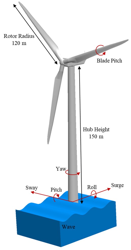
Figure 1: Rotation and movement axes, and dimensions of the IEA $15$ MW reference wind turbine in an offshore environment.

Table 1: Primary design parameters of the IEA $15$ MW reference wind turbine model

Parameter	IEA 15-MW Turbine	Unit
Power Rating	15	MW
Specific Rating	332	W/m2
Number of Blades	3	-
Cut-in Wind Speed	3	m/s
Rated Wind Speed	10.59	m/s
Cut-out Wind Speed	25	m/s
Rotor Diameter	240	m
Airfoil Series	FFA-W3	-
Hub Height	150	m
Hub Diameter	7.94	m
Hub Overhang	11.35	m
Drivetrain	Low Speed Direct Drive	-
Design Tip-Speed Ratio	90	-
Minimum Rotor Speed	5	rpm
Maximum Rotor Speed	7.56	rpm
Maximum Tip Speed	95	m/s
Blade Mass	65	t
Rotor Nacelle Assembly Mass	1017	t
Tower Mass	860	t
Tower Base Diameter	10	m
Monopile Base Diameter	10	m
Monopile Mass	1318	t
Monopile Embedment Depth	15	m

2.3 Surrogate Modeling of Stochastic Simulators Using Gaussian Process Regression

The stochastic simulation results of OpenFAST are analyzed using Gaussian process (GP) regression. GPs have shown tremendous successes in the last decade to model the outputs from complex computer simulations in physical and engineering sciences, mostly owing to their flexibility to characterize complex nonlinear response surfaces [31]. For example, they have been used as surrogates to approximate the response of hydrodynamics in San Francisco Bay for coastal protection infrastructure [27, 28], and to forecast local wind fields in onshore wind farms [32]. Here, we employed a GP with automatic relevance determination [33], which naturally factors in the relative importance of the input variables into the regression model. Details about the mathematical foundations of GPs, and model training procedure, are deferred to Appendix B.

3 Results

We first present our model validation diagnostics of the OpenFAST simulations for the $15$ MW reference turbine, then proceed to conduct an exploratory analysis on the resulting stochastic simulations. An exhaustive sensitivity analysis is then performed to infer the impact of several environmental inputs on the offshore power and identify the most informative combination of inputs in light of the out-of-sample prediction accuracy. Finally, a case study is presented, wherein the trained models are evaluated using real-world offshore measurements from the New York/New Jersey Bight.

3.1 Validation of OpenFAST for the $15$ MW Reference Turbine Design

While OpenFAST has been validated in numerous studies for the $5$ MW NREL reference offshore wind turbine, its applicability to the new IEA $15$ MW turbine is not yet established. Here, we validate our OpenFAST simulation results using the nominal power curve for the steady-state performance of the turbine rotor presented in the NREL technical report [23]. As the simulations in OpenFAST are transient, a total of $300$ seconds is modeled for each case and we only select the last $60$ seconds for analysis. The results have been visually examined for each case to ensure the spin-up time was not included in the data analysis. An example for the power output is illustrated in Fig. 2. In Fig. 3, the time-averaging results are compared with the NREL technical data. As shown in Fig. 3(a) and (b), the variations of generator power and torque with wind speed obtained from the stochastic simulations are in good agreement with the NREL data. In addition, the variations of rotor angular speed and blade pitch angle with the wind speed are plotted in Fig. 3(c) and (d).

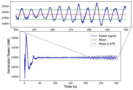
Figure 2: Generator power variations during a $300$-second simulation. As depicted, we only select the mean and standard deviation for the last $60$ seconds.

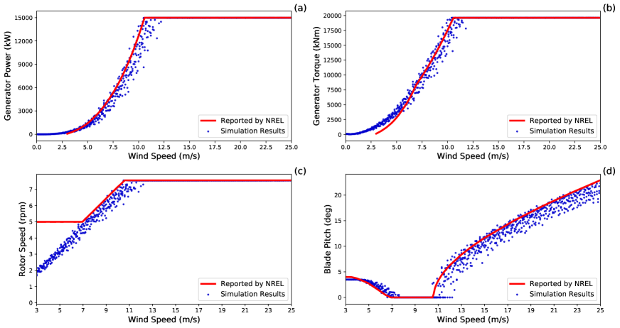
Figure 3: Comparison of steady-state values of the (a) generator power, (b) generator torque, (c) rotor speed, and (d) blade pitch angle with the data reported by NREL [23].

It can be seen that for the rotor speed variations, there is a discrepancy between NREL data and steady-state results for wind speeds less than $7$ m/s. This difference can be attributed to the performance of the NREL Reference Open-Source Controller (ROSCO) [34] implemented in OpenFAST. In ROSCO, two proportional integral (PI) controllers for generator torque and blade pitch angle are actively running to ensure the wind turbine is operating within safe conditions under the design constraints, so the rotational speed of the turbine rotor is constrained to $5$ rpm and above [23].

3.2 Exploratory Analysis of Wind Power Variability in Complex Environments

Wind speed is known to be the major determinant of offshore wind power, but other factors may exhibit a secondary, yet significant effect. This secondary effect is often overshadowed by the significant impact of wind speed variability on wind power. To examine the impact of other environmental factors, we specifically highlight four cases which have similar (almost identical) wind speeds of approximately $10.9$ m/s. Those are denoted hereinafter as Cases 1-4, and are depicted in Fig. 4. The environmental conditions for these cases are listed in Table 2.

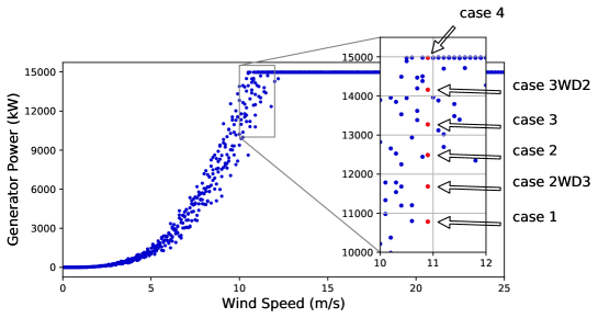
Figure 4: Results from OpenFast simulations depicting wind speed versus the resulting wind power. Inset highlights Cases $1$-$4$ which have similar wind speeds, but substantially different environmental conditions

Table 2: The environmental conditions for the four cases used for time series comparison

Case	Wind	Wind	Wave	Wave	Air	Air	Relative	Air
	Speed	Direction	Height	Direction	Pressure	Temperature	Humidity	Density
	(m/s)	(deg)	(m)	(deg)	(Pa)	(∘C)	(%)	(kg/m3)
1	10.9	28.3	2.4	111.4	97011	13.6	48.2	1.1756
2	10.9	16.9	1.3	78.8	97525	36.2	81.2	1.0778
3	10.9	20.8	5.2	129.6	111319	39.9	62.0	1.2200
4	10.9	5.8	13.3	70.1	104234	2.3	77.4	1.3162
3WD2	10.9	16.9	5.2	129.6	111319	39.9	62.0	1.2200
2WD3	10.9	20.8	1.3	78.8	97525	36.2	81.2	1.0778

OpenFAST results for these cases show that the generated power ranges from $10.8$ to as high as $15.0$ MW, with the maximum being $\sim 39\%$ higher than the minimum, suggesting that other environmental variables, in addition to wind speed, can have a significant impact on offshore power generation. A closer look reveals that two factors (other than wind speed) are dominant in determining the generator power: air density and relative wind direction. Specifically, by ranking the four cases according to their relative wind direction values, we can clearly see from Fig. 4 that Case 4 has the minimal relative wind direction value and the maximum wind power generation. This order is reversed for Case 1, suggesting an inverse relationship between relative wind direction and generated power (contingent on a constant wind speed). Along the spectrum, Cases 2 and 3 have intermediate relative wind direction values and consequently, their correspondent wind power values are both smaller than that of Case 4, but larger than that of Case 1. We note, however, that Case 3 generates higher power than that of Case 2, albeit having a slightly greater relative wind direction value. We conjecture that this can be explained by the difference in air density, mainly driven by a large difference in air pressure. It is noted that the differences in other factors such as air temperature and relative humidity are less significant. To test this conjecture, we added two more cases: Case 3WD2 similar to Case 3, but with the relative wind direction of Case 2, and Case 2WD3 similar to Case 2, but with the relative wind direction of Case 3. It can be seen in Fig. 4 that Case 2WD3 generates less power than Case 2 that is obviously because of greater yaw misalignment; however, Case 3WD2 generates approximately 14% higher power than Case 2 , suggesting that air pressure and temperature (and consequently, density) play key roles in describing offshore power generation even if wind speed and relative wind direction are similar in different conditions. This aligns with the physical knowledge from the power generation law $P=\frac{1}{2}C_{p}\rho AV^{3}$, where the air density depends on air pressure and temperature (See Eq. (1)), and the relative wind direction determines $V$.

Although it is obvious that wind speed is the most significant factor in determining mean power, it is still unclear that whether yaw misalignment or air density is the second important factor under different environmental conditions. Considering the ratio of partial derivative of mean generator power with respect to yaw misalignment to the partial derivative with respect to density, we can examine the relative significance of these factors in describing mean power variability. As detailed in Appendix A (See Eq. (A.10)), it can be shown that the absolute value of this ratio is $|(\partial P/\partial\theta)/(\partial P/\partial\rho)|=3\rho tan(\theta)$. Hence, the importance of the variable depends on whether the ratio is greater or less than 1. Given that widest possible ranges of values are considered in the simulations, if the maximum and minimum air density in our dataset are substituted for in the ratio’s expression, two thresholds can be obtained for yaw misalignment as follows:

$$\theta_{1} =\arctan\left(\frac{1}{3\rho_{max}}\right)=12.34~{}\textrm{deg}$$ (2)

$$\theta_{2} =\arctan\left(\frac{1}{3\rho_{min}}\right)=18.36~{}\textrm{deg},$$

wherein if $\theta$ is less than $\theta_{1}$, it is guaranteed that the significance of density is higher than yaw misalignment, while if $\theta$ is greater than $\theta_{2}$, the generator power variability is more influenced by yaw misalignment rather than density. The cases with relative wind direction values between these two thresholds indicates the significance of density and yaw misalignment in predicting mean power variability are in the same order. It should be noted that in the whole dataset the number of cases with the ratio less than 1 is approximately the same as the number of cases with the ratio greater than 1. Therefore, using this analysis we cannot conclude which factor is the second dominant factor in describing wind power variability throughout the whole dataset. This is one of the limitations in conventional methods, thereby motivating the use of a data-driven approach particularly GP, which is able to infer the relative significance of input variables.

3.3 Global Sensitivity Analysis using GPs

To collectively estimate the impact of all seven environmental variables on the generator power, we seek a statistical data-driven approach using GPs to statistically infer the sensitivity of the power output to the environmental factors. The idea here is to train multiple GP models on different combinations of the environmental variables, using the OpenFAST simulation data. The relative importance of the input variables is inferred by the correspondent change of the GP-based prediction errors with and without a particular variable. We adopt a $10$-fold cross validation scheme and use three error metrics to evaluate the prediction errors, namely: the Mean Absolute Error (MAE), Root Mean Square Error (RMSE), and Normalized Root Mean Squared Error (NRMSE). which are expressed in Eqs (3)-(5).

$$\textrm{MAE}=\frac{1}{n}\displaystyle\sum_{i=1}^{n}|y_{i}-\hat{y}_{i}|,$$ (3)

$$\textrm{RMSE}=\sqrt{\frac{1}{n}\displaystyle\sum_{i=1}^{n}(y_{i}-\hat{y}_{i})^{2}},$$ (4)

$$\textrm{NRMSE}=\frac{1}{\tilde{y}}\sqrt{\frac{1}{n}\displaystyle\sum_{i=1}^{n}(y_{i}-\hat{y}_{i})^{2}},$$ (5)

where $y$ and $\hat{y}$ denote the actual value and prediction of the predictand, respectively, while $\tilde{y}$ is a reference value, which will be specified depending on the response of interest (more details in Sections 3.3.1 and 3.3.2).

Table 3: Prediction errors for different multivariate power curve models in terms of averaged MAE, RMSE, and NRMSE in 10-fold cross validation

No.	Models	$MAE_{avg}$	$RMSE_{avg}$	$NRMSE_{avg}$
		(kw)	(kw)	(%)
1	Simple Binning	243.1	571.3	3.81
2	Method of Bins (IEC Standard 61400–12-1)	207.0	488.0	3.25
3	$GP(V)$	240.6	529.2	3.53
4	$GP(V,\theta)$	149.1	333.7	2.22
5	$GP(V,\theta,T)$	120.5	257.6	1.72
6	$GP(V,\theta,T,P)$	30.9	78.3	0.52
7	$GP(V,\theta,T,P,\phi)$	31.0	78.8	0.53
8	$GP(V,\theta,T,P,\rho)$	23.1	60.3	0.40
9	$GP(V,\theta,T,P,\rho,H)$	24.6	63.7	0.42
10	$GP(V,\theta,T,P,\rho,H,\beta)$	23.3	60.6	0.40
11	$GP(V,\theta,\rho)$	23.1	60.3	0.40

3.3.1 First-order properties: The sensitivity of the mean power output to the environmental variables

To elucidate the effect of individual environmental inputs, a set of GP models is trained to the mean power output from the stochastic simulations, where, in addition to wind speed, we incrementally add the other environmental variables, one by one. We also include two benchmarks to compare against: simple binning and the standard method of bins. Simple binning takes wind speed as the sole input, and divides its domain into bins of $0.5$ m/s, which is the standard bin width in power curve estimation studies, and then takes the average of the power values within each bin as the estimated power. The method of bins, on the other hand, is similar to the binning method, but indirectly takes air density into account by performing a density correction to the wind speed values, as recommended by the IEC standard 61400-12-1 [12].

Table 3 shows the final prediction errors of all models, across the three metrics of Eqs (3)-(5). For NRMSE, we use the rated power as the reference value, that is, $\tilde{y}=P_{rated}=15,000$ kW. In general, as more input variables are added, prediction errors gradually decrease, except for the cases where adding relative humidity, wave height or wave direction, leads to a slight increase in prediction error. This is further illustrated in Fig. 5, which depicts the boxplots of the NRMSEs, across the $10$ folds, for each model. Looking at Table 3 and Fig. 5, we can infer the following key insights.

First, it can be seen that the standard method of bins achieves a noticeable improvement of $14.6\%$ in comparison with simple binning. It is also shown that, by leveraging the local correlation structure in the input space, a GP model with wind speed as the sole input, denoted by $GP(V)$, outperforms the simple binning method ($\sim 7.4\%$ improvement in NRMSE), but still falls short to the standard method of bins, which indirectly augments the input space via its embedded density correction. This finding indicates that, even advanced statistical approaches like GPs may not be able to provide significant competitive advantages over traditional approaches when solely using the wind speed as the only input—a conclusion which is largely overlooked in the literature, barring few recent works [15, 13]. This aligns with our findings from the exploratory analysis in Section 3.2, and highlights the importance of considering other environmental variables in addition to wind speed in characterizing offshore wind power.

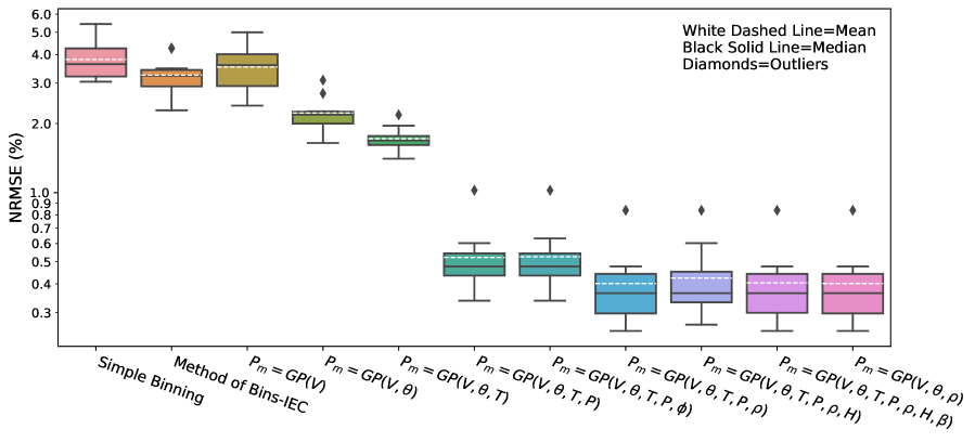
Figure 5: Boxplots of the NRMSEs of the mean power output predictions, across the 10 folds, for the $11$ different models thus considered.

Second, by using a GP model with wind speed and relative wind direction as input variables, a significant improvement ($\sim 31.7\%$) in comparison with the method of bins is observed, indicating that relative wind direction plays a key role in describing the mean power output, which again, coincides with our exploratory analysis in Section 3.2. By training a four-variable GP model and considering air temperature and pressure, $GP(V,\theta,T,P)$, significantly higher accurate predictions are further achieved ($76\%$ improvement in NRMSE relative to the method of bins). The best five-variable model is $GP(V,\theta,T,P,\rho)$, which achieves a final NRMSE of $0.4$, which is $23\%$ better than its four-input predecessor, and up to $88\%$ better than the method of bins. Although density is highly correlated to air pressure and temperature, we speculate that the realized improvement may be attributed to the fact that density can further capture the interaction effects of temperature and pressure. We alo note that adding wave height and wave direction does not lead to any significant improvements in predictive performance, concluding that the wind-related variables are the dominating environmental factors in describing the mean power output, while, on the other hand, the wave properties do not have a significant contribution, which is, perhaps, unsurprising.

Third, as thoroughly described in Appendix B, we employed an ARD-SE covariance function (See Eq. B.12), in which the estimated values for length-scale parameter $(\ell)$ can reveal the importance of each input variable, such that smaller value (or higher inverse values) of $\ell$ suggests higher significance. By normalizing 1/$\ell$ values, the contribution of each variable in three select GP models are listed in Table 4. For all three models, wind speed and yaw misalignment have the first and second highest importance with contributions of about $92\%$ and $5\%$, respectively. Furthermore, it can be inferred that in the $GP(V,\theta,T,P)$ model the importance of air pressure is slightly higher than air temperature. Also, it can be seen that, once density ins included in $GP(V,\theta,T,P,\rho)$ model, its contribution is about $3\%$, while the contributions of air temperature and pressure drop to around zero. This means that density appears to effectively encapsulate the combined impact of air pressure and temperature, and indicates that the best model is $GP(V,\theta,\rho)$, which (i) achieves the best performance in terms of prediction error across all metrics ($\sim 88\%$ reduction in NRMSE relative to the method of bins), (ii) is well aligned with the physical law of power generation, and (iii) is further in line with the law of parsimony in statistical and machine learning, particularly when compared against other model representations with more variables (and hence higher complexity), but offer no competitive advantage in terms of prediction accuracy.

Table 4: Inverse of length-scale parameter $(\ell)$ and the percentage of the importance of input variables in GP regression

	$GP(V,\theta,T,P)$			$GP(V,\theta,T,P,\rho)$			$GP(V,\theta,\rho)$
Input Variable	1/$\ell$	%		1/$\ell$	%		1/$\ell$	%
Wind Speed $(V)$	5.921	92.6		6.656	91.92		6.656	91.92
Yaw Misalignment $(\theta)$	0.309	4.84		0.368	5.09		0.368	5.09
Air Pressure $(P)$	0.091	1.43		$1\text{\times}{10}^{-6}$	$\approx 0$		-	-
Air Temperature $(T)$	0.067	1.06		$5\text{\times}{10}^{-6}$	$\approx 0$		-	-
Air Density $(\rho)$	-	-		0.216	2.99		0.216	2.99

3.3.2 Second-order properties: The sensitivity of the variance in power output to the environmental variables

The second order properties of the power output, defined in this paper as the variation of the power around its mean, is an important, but often overlooked, quantity in power curve estimation studies. As a case in point, the high variance in power output can cause significant disruptions to grid integration and energy storage. Moreover, it contributes to structural fatigue, foundation instability, and marine noise pollution. The IEC Standard 61400–12-2 suggests that the uncertainty in the power curve may be on the order of $10$% or more, depending on site conditions and climate [35]. Understandably, the uncertainty may be affected by a combination of several environmental factors. Here, we seek to infer the impact of these factors on the variation of the power output around its mean behavior by analyzing the results of the stochastic simulations generated by OpenFAST.

To motivate the analysis, we particularly highlight three simulated cases that have identical wind speeds, and approximately the same mean power output, yet they exhibit extremely different behaviors in terms of the variability around that mean. Fig. 6 shows sample results for the time variations in the power output and the three displacements of the turbine platform, namely roll, pitch, and blade pitch angle for these three cases. The definition of the rotational displacements are depicted in Fig. 1. The table in the top panel of Fig. 6 shows the values of the relevant environmental variables for these three cases. As can be seen in Fig. 6, the case in which the turbine experiences stronger displacement fluctuations has larger periodic variations around the mean power output. Interestingly, we observe that the amplitude of these power variations may be positively correlated with wave height, $H$, that is, larger wave heights correspond to more severe power variations.

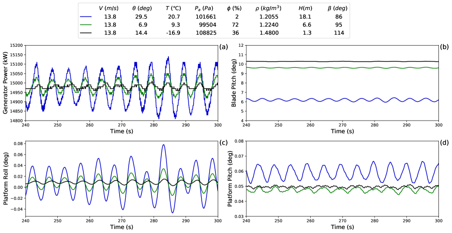
Figure 6: Fluctuations of (a) output power, and the variations of turbine (b) blade pitch, (c) platform roll, and (d) platform pitch during one-minute for three cases with identical wind speed and mean output power

To test this conjecture, we perform a similar sensitivity analysis to that of Section 3.3.1. to study the second-order properties of power output. Here, we use the standard deviation of the generator power, denoted by $P^{sd}$, to quantify the second moment and the reference value used in NRMSE calculations is the maximum observed standard deviation in the training data, i.e. $\tilde{y}=\underset{i=1,...,n}{\max}P^{sd}_{i}$. The results, shown in Fig. 7, indicate that wind-related variables, alone, cannot explain the variance in the power output. Once the wave-related variables are added as inputs, the predictive performance is significantly improved. In particular, the model with wind speed, wave height, and wave direction, denoted by $GP(V,H,\beta)$, achieves $\sim 86\%$ improvement, in terms of NRMSE, over the model which uses wind speed as the sole input, namely $GP(V)$. Minor to null improvements are achieved by adding additional variables beyond those three variables, which, again, is well aligned with the law of parsimony. This analysis interestingly suggests that wave-related variables are significant contributors to the power output uncertainty in offshore environments, whether as individual effects, or as interaction with the wind speed variable. At the first glance, the strong importance of the wave effects may be a little surprising since they are insignificant in characterizing the mean power output, as shown in Section 3.3.1. This finding can be explained by the fact that periodic waves are the only dynamic forcing among all the environmental variables under consideration.

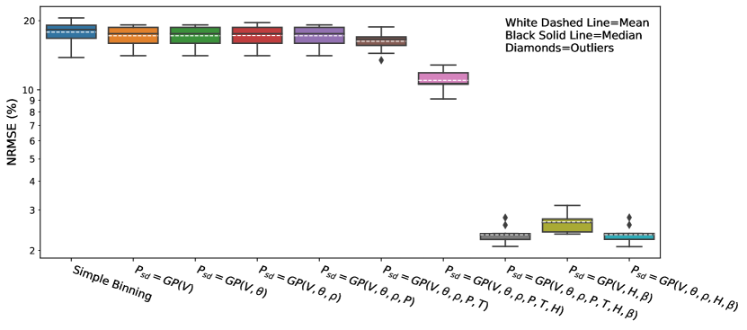
Figure 7: Boxplots for the distributions of normalized root mean square errors in 10-fold cross validation training and predicting generator power standard deviation for different multivariate GP models and simple binning method.

In addition to $GP(V,H,\beta)$ which demonstrates a satisfactory performance in predicting the second order properties of the power output, we develop a second-order effect curve, a counterpart to the “power curve” in Fig. 4, which is based on fractional polynomial regression equation, shown in Eq.(6), for which the parameters are estimated using non linear least squares.

$$\left[\frac{P^{sd}}{\frac{1}{2}{\rho}A{V_{cutout}^{3}}}\right]=-2.63+2.78{\mathit{\left(\frac{V}{V_{cutout}}\right)}}^{0.37}+1.81{\left(\frac{\mathit{H}}{\sqrt{A}}\right)}^{1.21}-{1.02}{\mathit{\beta}}^{4.86},$$ (6)

where $P^{sd}$ is the standard deviation of the generator power. The corresponding $10$-fold NRMSE of this model is $13.44\%$, which is still $\sim 22\%$ better than that of $GP(V)$, albeit substantially higher than $GP(V,H,\beta)$. The main reason of introducing this model is its interpretability and ease of use, which may counterbalance its lower accuracy relative to $GP(V,H,\beta)$. From the fitted equation, we can note that the three factors have notable impact on $P^{sd}$, as evident by the estimated parameter values.

Note that the present study focuses on the seven selected environmental factors, without including the effects of wind turbulence, shearing, and vaning, etc, so the strong wave effect may be less important than those dynamic forces in the offshore environment, which is indeed a topic of future research. We also stress that the present study is restricted to the dynamics that have been implemented in the OpenFAST framework, so any observation here is limited by the assumptions made in the OpenFAST framework. In turn, the developed GPs have the same limitations as OpenFAST, because the GPs are trained based on the OpenFAST results. But the limitations of the GPs are not permanent due to the independence between OpenFAST and GPs – we expect that improved simulations or rich field observation data can reduce the limitation of the GPs. The analysis above reveals the potentially significant impact of ocean waves on the steadiness of the power output. The magnitude of the absolute fluctuation observed here can be compared with future studies focusing on the fluctuation introduced by wind turbulence, shearing, and vaning to identify the most influencing set of environmental variables. To the knowledge of the authors, this is the first attempt in a scientific study to particularly analyze, in depth, the determinants of the uncertainty in offshore power output, which can be potentially instrumental to grid integration and energy storage decisions.

3.4 Case Study: Application to Real-world Data from the New York/New Jersey Bight

In this section, the best-performing models from Sections 3.3.1 and 3.3.2 for the prediction of mean and standard deviation of generator power, respectively, are applied to a real-world dataset collected using the E06 Hudson South LiDAR buoy, which is one of the buoys deployed by NYSERDA (New York State Energy Research & Development Authority), strategically located in proximity to at least 3 future offshore wind farm locations, a few miles off the New Jersey and New York shorelines ($39^{o}32^{\prime}48.38"$N, $73^{o}25^{\prime}44.01"$W). Wind and wave data are collected, at multiple altitudes, since September 2019, and are made publicly available by NYSERDA [36]. Here, we focus on a 7-day period from September 20th to 27th, 2019, which includes $10$-minute measurements of the wind speed at the height of $158$ m (nearest height to the turbine hub height), air temperature, atmospheric pressure, and relative humidity. In addition, $1$-hour measurements of the wave height and wave direction are available during the same period. As shown in Fig. 8(a), the wind speed during this period has a clear daily cycle. The weather experienced an early temperature and humidity rise, accompanied by a low pressure system in the later part of the 7-day period. Wave heights were mostly moderate with a visible shift in wave direction taking place approximately during the fourth day.

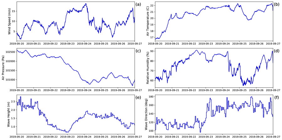
Figure 8: Variations of environmental variables during the $7$-day period recorded from NYSERDA’s buoy dataset, including: a) wind speed, b) air temperature, c) air pressure, d) relative humidity, e) wave height, and d) wave direction.

The input data for OpenFAST can be determined using the buoy’s field data, except for one variable: the relative wind direction (or yaw misalignment), since no wind farms exist yet at this location. Gaumond et al. [37] suggested that the yaw misalignment is highly correlated with the second-order behavior of wind direction. This is due to the design of yaw controllers in modern-day horizontal wind turbines in avoiding the instantaneous tracking of incoming wind directions. In other words, if the wind direction varies more frequently and with higher amplitude, a wind turbine will experience greater yaw misalignment degrees. Hence, to estimate the yaw misalignment, we need to assess the standard deviation within $10$-minute periods (The $10$-min sampling frequency of the NYSERDA data is too coarse). To address this issue, we used an additional database – the 1-Hz dataset collected by AXYS Wind Sentinel Buoy Lidar [38, 39], which was deployed by Pacific Northwest National Laboratory (PNNL) from November 2015 to February 2017 in the New Jersey offshore area about 3 miles off the coast of Atlantic City, relatively near to the NYSERDA buoy location. Specifically, we used this dataset for analyzing wind direction variations in the same 7-day period in 2016, shown in Fig. 9(a). The standard deviation of each 10-minute interval is calculated and plotted in Fig. 9(b), which will be used as a proxy for relative wind direction (or yaw misalignment). The probability density of the yaw misalignment values is shown in Fig. 9(c), where most values are in the range of 0-30 degree.

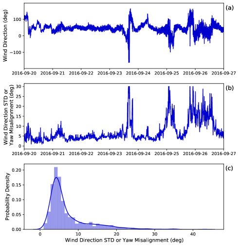
Figure 9: Analysis of the $1$-Hz AXYS Wind Sentinel Buoy data: (a) Time series of the wind direction, b) $10$-min wind direction standard deviation. c) Probability density of the wind direction standard deviation.

3.4.1 Case Study Results

OpenFAST is used to simulate the power generation for the buoy’s location during the $7$-day period of interest. The GP models are then trained to the resulting simulation outputs. Fig. 10(a) and (b) show the power curves obtained by the method of bins and the best-performing GP model, respectively. Fig. 10(b) shows that the generator power values predicted by the best three-variable GP model, namely $GP(V,\theta,\rho)$ are in excellent agreement with those obtained by OpenFAST, meaningfully better than the method-of-bins model, especially in the middle region of the power curve, i.e., at wind speeds less than the turbine rated speed ($10.6$ m/s) and greater than $8.0$ m/s.

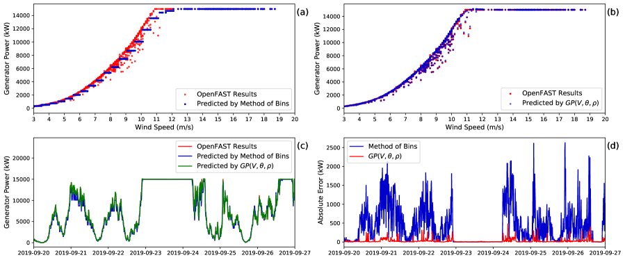
Figure 10: Comparison between OpenFAST simulation results and generator power values predicted by (a) method of bins, and (b) Gaussian Processes model of $GP(V,\theta,\rho)$; (c) Time series of generator power simulated by OpenFAST versus those predicted by the method of bins and $GP(V,\theta,\rho)$; (d) Time series of the absolute errors from $GP(V,\theta,\rho)$ versus those from the method of bins.

Fig. 10(c) shows the time series of the generator power values simulated via OpenFAST, versus those predicted from the method-of-bins and $GP(V,\theta,\rho)$. The times series of the absolute errors of the two models are shown in Fig. 10(d), in which $GP(V,\theta,\rho)$ is shown to be $91\%$ more accurate than the method of bins, in terms of NRMSE. In terms of energy production, the total output energy predicted by OpenFAST over the one-week period is about 1347 MWh, while the total absolute energy error of the GP and method-of-bins relative to the OpenFAST total output energy are $4.6$ and $68.0$ MWh, respectively. Note that the selected period is not necessarily exhaustive nor representative of the life cycle of the wind turbine, and hence, we expect that the total energy prediction error may change in other weeks, seasons, or years. The improvement in predictive performance achieved by the multi-input GP over the method of bins can be significant in industrial applications, and hence, we conclude that considering the environmental variables in addition to the wind speed, particularly the relative wind direction and air density, can significantly improve the prediction of offshore wind power.

In addition, the standard deviation of the generator power is predicted for the same period using $GP(V,H,\beta)$. The power uncertainty counterpart of the power curve for the $7$-day period is shown in Fig. 11(a). The GP-based predictions show a decent agreement with OpenFAST simulations, albeit not as good as those shown for the mean power prediction, which is expected. Particularly, we note that the prediction errors are higher at wind speeds in the range of $6$ to $10$ m/s. In Fig. 11(b), the time series of the generator power standard deviation simulated by OpenFAST are shown against those predicted by the multi-input GP model. By comparing this Figure with Fig. 10(c), it can be seen that during the time when the turbine generates the rated power, the predicted values of power standard deviation have the lowest errors, which, again, is unsurprising.

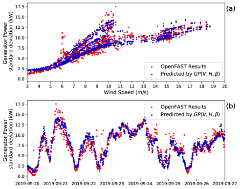
Figure 11: Comparison between the OpenFAST results and GP-based predictions for (a) different wind speeds, and (b) versus time.

The case study shows that the statistical models proposed herein are well-suited to accurately predict the first two moments of the offshore power output. It also suggests that carefully integrating more environmental variables can result in substantial improvements to the prediction accuracy. We envision our analysis to be particularly relevant to the growing offshore wind industry since an accurate prediction of the mean power output is known to be instrumental for productivity assessment, and for turbine- and farm-level operational activities. On the other hand, the capability to accurately assess the variation of the offshore power output around its mean, i.e. its second-order properties, can prove extremely useful to critical farm-level decisions, such as integration steadiness with the grid, and management of energy storage systems, both of which are of increasing importance in light of the growing scale and sophistication of modern-day offshore wind farms.

4 Conclusion

In this study, we performed an exhaustive sensitivity analysis to reveal the impact of atmospheric and marine conditions on the first and second-order properties of offshore wind power. We coupled Gaussian Processes (GPs), a nonparametric statistical learning approach, with OpenFAST, a high-fidelity physics-based simulator, to reproduce, and further predict the design power curve of a 15 MW wind turbine. The analysis revealed that in addition to wind speed, air density and relative wind direction are instrumental in predicting the mean offshore power output, yielding substantial improvements relative to the method of bins. In addition, the impact of wave-related variables on the second-order properties of offshore wind power is, for the first time, elucidated, potentially providing valuable information to power grid integration and storage decisions. OpenFAST is also found suitable to predict the power fluctuation that the traditional power curve cannot capture. Tested on actual offshore measurements from the New York/New Jersey bight, the GP-based models showed significant improvements over the method of bins in predicting the mean and standard deviation of offshore wind power, motivating a need, for both the research community and practitioners in the offshore wind industry, to shift towards multi-input statistical characterizations for offshore wind power assessment and prediction, especially in complex marine environments.

This study will serve as an anchor point for future research along several directions. For instance, few environmental parameters are missing in the presented modeling and analysis. We plan to fill the gap in the future by extending our analysis to include the effects of turbulence characteristics, vaning, and shearing. In addition, due to the limitation of OpenFAST, the coupling among the dynamics of underwater structure, the turbine, and surface structures is still missing. This may lead to an underestimate of the second-moment dynamics due to waves and related parameters. We expect future updates of OpenFAST to improve this aspect to allow a fully coupled modeling study. At last, it will be beneficial to engage field data to further validate the discovery of this paper and our team is currently exploring opportunities along this direction.

Appendix A

Using the derivatives of the fundamental wind power equation, the significance of its input variables in predicting mean wind power can be estimated given the ranges of the input variables.

$$P=\frac{1}{2}C_{p}\rho AV^{3}=\frac{1}{2}C_{p}\rho AV^{3}cos^{3}(\theta)$$ (A.7)

$$\frac{\partial P}{\partial\theta}=-\frac{3}{2}C_{p}\rho AV^{3}sin(\theta)cos^{2}(\theta)$$ (A.8)

$$\frac{\partial P}{\partial\rho}=\frac{1}{2}C_{p}AV^{3}cos^{3}(\theta)$$ (A.9)

The absolute value of the ratio of those derivatives, derived in Eq. (A.10), can reveal insights about the relative importance of density and relative wind direction in predicting mean wind power by Eq. (A.7).

$$\left\lvert\frac{\partial P/\partial\theta}{\partial P/\partial\rho}\right\rvert=\frac{\frac{3}{2}C_{p}\rho AV^{3}sin(\theta)cos^{2}(\theta)}{\frac{1}{2}C_{p}AV^{3}cos^{3}(\theta)}=3\rho\;tan(\theta)$$ (A.10)

Appendix B

The set of environmental inputs, which is used to explain the variability in the offshore power output $P$, is denoted by $\mathbf{x}\in\mathbb{R}^{p}$. At our disposal is a set of input-output training data, wherein $[\mathbf{x}_{1},...,\mathbf{x}_{n}]^{T}$ is the $n\times p$ matrix of training data inputs, and $\mathbf{P}=P(\mathbf{x}_{1},...,\mathbf{x}_{n})=[P_{1},...,P_{n}]^{T}$ is the $n\times 1$ vector of correspondent target values (power mean or standard deviation) collected from the output of the stochastic simulations. The goal of GPs (and of any statistical regression method) is to construct the unknown functional response governing the relationship between $\mathbf{x}\in\mathbb{R}^{p}$ and $P$ using the training data. GPs can be written in the additive form of Eq. (B.11)

$$P_{i}=\mu(\mathbf{x}_{i})+\xi(\mathbf{x}_{i}),$$ (B.11)

where $\mu(\mathbf{x}_{i})$ is often called mean function, while $\xi(\mathbf{x}_{i})$ is a dependent error term. The mean function can be modeled either as a constant, or as a parametric function of the inputs $\mathbf{x}$, such that $\mu(\mathbf{x}_{i})=\mathbf{x}_{i}\boldsymbol{\beta}$, where $\mathbf{x}_{i}$ is the $1\times p$ vector of regression inputs and $\boldsymbol{\beta}$ is a $p\times 1$ vector of regression coefficients.

The dependent error term $\xi(\mathbf{x}_{i})$ is defined as a zero mean Gaussian random field, with an $n\times n$ covariance matrix denoted by $\boldsymbol{\Sigma}$, for which each entry represents a measure of covariance (or similarity) between a pair of data points. The entries of $\boldsymbol{\Sigma}$ can be determined via an isotropic covariance function (or a kernel) $K(\cdot,\cdot)$. Covariance functions play a critical role in GP regression, especially for modeling complex physical processes [40]. A popular choice for $K(\cdot,\cdot)$ is the automatic relevance determination squared exponential (ARD-SE) kernel, which is expressed as in Eq. (B.12).

$$K_{\text{ARD-SE}}(\mathbf{x}_{i},\mathbf{x}_{j})=\sigma_{f}^{2}\exp\bigg{[}-\frac{1}{2}\sum_{k=1}^{p}\frac{(\mathbf{x}_{ik}-\mathbf{x}_{jk})^{2}}{\ell_{k}^{2}}\bigg{]}+\sigma_{n}^{2}\mathbb{I}({i=j}),$$ (B.12)

where $\mathbf{x}_{ik}$ and $\mathbf{x}_{jk}$ denote the value of the $k$th environmental input for data points $i$ and $j$, respectively. The parameter $\sigma_{f}^{2}$ denotes the marginal variance parameter, while $\sigma_{n}^{2}$ denotes the noise variance to reflect the stochastic nature of the simulations, such that $\mathbb{I}(\cdot)$ is the indicator function (i.e. $\mathbb{I}(i=j)=1$ when $i=j$ and $0$ otherwise). The parameters $\ell_{1},...,\ell_{p}$ are called the length-scale parameters, for which the estimated values can be used to infer the importance of input variables, i.e. smaller values indicate higher importance (or relevance), and hence is the term automatic relevance determination in the GP literature [33].

Combined, the regression coefficients of the mean function and the covariance parameters form the vector of GP parameters $\boldsymbol{\Theta}=\{\boldsymbol{\beta},\sigma_{f}^{2},\ell_{1},...,\ell_{p},\sigma_{n}^{2}\}$, which can be estimated in a data-driven way by maximizing (minimizing) the (negative) log-likelihood of the GP model. This can be realized numerically using gradient-descent based optimization. Once the set of parameters has been estimated, encapsulated in the vector $\hat{\boldsymbol{\Theta}}$, they form the basis for the GP-based predictions, which can be expressed as in Eq. (B.13).

$$\hat{P}(\mathbf{x}^{*})=\mathbb{E}[P(\mathbf{x}^{*})|P_{1},...,P_{n}]=\mu(\mathbf{x}^{*})+\hat{\mathbf{k}}^{T}\hat{\boldsymbol{\Sigma}}^{-1}(\mathbf{P}-\boldsymbol{\mu}),$$ (B.13)

where $\hat{P}(\mathbf{x}^{*})$ is the predicted target value at any arbitrary input point $\mathbf{x}^{*}$, while $\hat{\boldsymbol{\Sigma}}$ is the estimated covariance matrix using $\hat{\boldsymbol{\Theta}}$. The $n\times 1$ vector $\hat{\mathbf{k}}$ denotes the vector of covariances between $\mathbf{x}^{*}$ and $[\mathbf{x}_{1},...,\mathbf{x}_{n}]^{T}$, while $\boldsymbol{\mu}=\mu(\mathbf{x}_{1},...,\mathbf{x}_{n})$ is the $n\times 1$ vector of mean function evaluations at the training data.

For the analysis in this paper, we have implemented our own version of the GP regression model. For parameter estimation, the negative log-likelihood was minimized using the gradient descent-based minimization with an iteration limit set at $300$. Setting $\mu(\mathbf{x})$ to zero appeared to return satisfactory predictive performance for all the GP models considered herein.

References

-
[1]
IEA, Offshore Wind Outlook 2019,
(Accessed on 07/20/2020).
URL https://www.iea.org/analysis -
[2]
T. Johnson,
New
York tops NJ with plans for offshore wind, (Accessed on 07/10/2020).
URL https://www.njspotlight.com/2019/07/19-07-18-new-york-tops-nj-with-plans-for-offshore-wind/ - [3] D. Sheppard, N. Thomas, National grid electricity blackout report points to failure at wind farm, https://www.ft.com/content/8b738eac-c024-11e9-89e2-41e555e96722, (Accessed on 03/25/2021) (Aug 2019).
- [4] B. K. Sullivan, N. S. Malik, Texas power outage: 5 million affected after winter storm, https://time.com/5939633/texas-power-outage-blackouts/, (Accessed on 03/25/2021) (Feb 2021).
- [5] B. Niu, H. Hwangbo, L. Zeng, Y. Ding, Evaluation of alternative power production efficiency metrics for offshore wind turbines and farms, Renewable Energy 128 (2018) 81–90.
- [6] S. Gill, B. Stephen, S. Galloway, Wind turbine condition assessment through power curve copula modeling, IEEE Transactions on Sustainable Energy 3 (1) (2011) 94–101.
- [7] T. Ouyang, A. Kusiak, Y. He, Modeling wind-turbine power curve: A data partitioning and mining approach, Renewable Energy 102 (2017) 1–8.
- [8] A. A. Ezzat, M. Jun, Y. Ding, et al., Spatio-temporal short-term wind forecast: a calibrated regime-switching method, The Annals of Applied Statistics 13 (3) (2019) 1484–1510.
- [9] P. Gebraad, J. J. Thomas, A. Ning, P. Fleming, K. Dykes, Maximization of the annual energy production of wind power plants by optimization of layout and yaw-based wake control, Wind Energy 20 (1) (2017) 97–107.
- [10] M. F. Howland, S. K. Lele, J. O. Dabiri, Wind farm power optimization through wake steering, Proceedings of the National Academy of Sciences 116 (29) (2019) 14495–14500.
- [11] P. Papadopoulos, D. Coit, A. A. Ezzat, Seizing opportunity: Maintenance optimization in offshore wind farms considering dispatch, accessibility, and production, Available at https://arxiv.org/abs/2012.00213 (2020). arXiv:2012.00213.
- [12] IEC, Wind turbines-part 12-1: Power performance measurements of electricity producing wind turbinesIEC-International Electrotechnical Commission, IEC-61400-12, Geneva, Switzerland (2005).
- [13] R. K. Pandit, D. Infield, J. Carroll, Incorporating air density into a gaussian process wind turbine power curve model for improving fitting accuracy, Wind Energy 22 (2) (2019) 302–315.
- [14] J. Jeon, J. W. Taylor, Using conditional kernel density estimation for wind power density forecasting, Journal of the American Statistical Association 107 (497) (2012) 66–79.
- [15] G. Lee, Y. Ding, M. G. Genton, L. Xie, Power curve estimation with multivariate environmental factors for inland and offshore wind farms, Journal of the American Statistical Association 110 (509) (2015) 56–67.
- [16] J. M. Jonkman, A. D. Wright, G. J. Hayman, A. N. Robertson, Full-system linearization for floating offshore wind turbines in openfast, in: ASME 2018 1st International Offshore Wind Technical Conference, American Society of Mechanical Engineers Digital Collection, 2018.
- [17] N. Johnson, J. Jonkman, A. Wright, G. Hayman, A. Robertson, Verification of floating offshore wind linearization functionality in openfast, in: Journal of Physics: Conference Series, Vol. 1356, IOP Publishing, 2019, p. 012022.
- [18] R.-Q. Wang, T. N. Miles, J. F. Brodie, Multi-scale interaction between wind turbines and coastal processes: coupling openfast with a regional coupled air-sea modeling system, in: Ocean Sciences Meeting 2020, AGU, 2020.
- [19] A. Wise, E. E. Bachynski, Analysis of wake effects on global responses for a floating two-turbine case, in: Journal of Physics: Conference Series, Vol. 1356, IOP Publishing, 2019, p. 012004.
- [20] R. Fadaeinedjad, M. Moallem, G. Moschopoulos, Simulation of a wind turbine with doubly fed induction generator by fast and simulink, IEEE Transactions on energy conversion 23 (2) (2008) 690–700.
- [21] R. Tran, J. Wu, C. Denison, T. Ackling, M. Wagner, F. Neumann, Fast and effective multi-objective optimisation of wind turbine placement, in: Proceedings of the 15th Annual Conference on Genetic and Evolutionary Computation, GECCO ’13, Association for Computing Machinery, New York, NY, USA, 2013, p. 1381–1388. doi:10.1145/2463372.2463541.
- [22] H. Shariatpanah, R. Fadaeinedjad, M. Rashidinejad, A new model for pmsg-based wind turbine with yaw control, IEEE transactions on energy conversion 28 (4) (2013) 929–937.
-
[23]
E. Gaertner, J. Rinker, L. Sethuraman, F. Zahle, B. Anderson, G. Barter,
N. Abbas, F. Meng, P. Bortolotti, W. Skrzypinski, G. Scott, R. Feil,
H. Bredmose, K. Dykes, M. Sheilds, C. Allen, A. Viselli,
Definition of the IEA
15-megawatt offshore reference wind turbine, Tech. rep., International
Energy Agency (2020).
URL https://www.nrel.gov/docs/fy20osti/75698.pdf - [24] M. Schlechtingen, I. F. Santos, S. Achiche, Using data-mining approaches for wind turbine power curve monitoring: A comparative study, IEEE Transactions on Sustainable Energy 4 (3) (2013) 671–679.
- [25] Wind turbines – Part 1: Design requirements, Standard, IEC-International Electrotechnical Commission (2014).
-
[26]
I. Sobol’,
On
the distribution of points in a cube and the approximate evaluation of
integrals, USSR Computational Mathematics and Mathematical Physics 7 (4)
(1967) 86 – 112.
doi:https://doi.org/10.1016/0041-5553(67)90144-9.
URL http://www.sciencedirect.com/science/article/pii/0041555367901449 - [27] M. Li, R.-Q. Wang, G. Jia, Efficient dimension reduction and surrogate-based sensitivity analysis for expensive models with high-dimensional outputs, Reliability Engineering & System Safety 195 (2020) 106725.
- [28] G. Jia, R.-Q. Wang, M. T. Stacey, Investigation of impact of shoreline alteration on coastal hydrodynamics using dimension reduced surrogate based sensitivity analysis, Advances in Water Resources 126 (2019) 168–175.
- [29] B. Zhao, R.-Q. Wang, S. Cao, Modeling the cleaning cycle dynamics for air cooling condensers of thermal power plants: Optimization and global sensitivity analysis, submitted.
- [30] J. Jonkman, The new modularization framework for the fast wind turbine cae tool, in: 51st AIAA Aerospace Sciences Meeting including the New Horizons Forum and Aerospace Exposition, 2013, p. 202.
- [31] A. A. Ezzat, J. Tang, Y. Ding, A model-based calibration approach for structural fault diagnosis using piezoelectric impedance measurements and a finite element model, Structural Health Monitoring 19 (6) (2020) 1839–1855.
- [32] A. A. Ezzat, M. Jun, Y. Ding, Spatio-temporal asymmetry of local wind fields and its impact on short-term wind forecasting, IEEE transactions on sustainable energy 9 (3) (2018) 1437–1447.
- [33] C. K. Williams, C. E. Rasmussen, Gaussian processes for machine learning, Vol. 2, MIT press Cambridge, MA, 2006.
-
[34]
NREL, ROSCO. Version 1.0.0 (2020).
URL https://github.com/NREL/rosco - [35] IEC, Wind turbines-part 12-2: Power performance of electricity-producing wind turbines based on nacelle anemometryIEC-International Electrotechnical Commission, IEC 61400-12-2, Geneva, Switzerland (2013).
-
[36]
NYSERDA
Floating LiDAR Buoy Data, (Accessed on 03/01/2020) (2020).
URL https://oswbuoysny.resourcepanorama.dnvgl.com/download/f67d14ad-07ab-4652-16d2-08d71f257da1 -
[37]
M. Gaumond, P.-E. Réthoré, S. Ott, A. Peña, A. Bechmann, K. S. Hansen,
Evaluation of
the wind direction uncertainty and its impact on wake modeling at the horns
rev offshore wind farm, Wind Energy 17 (8) (2014) 1169–1178.
arXiv:https://onlinelibrary.wiley.com/doi/pdf/10.1002/we.1625, doi:10.1002/we.1625.
URL https://onlinelibrary.wiley.com/doi/abs/10.1002/we.1625 - [38] K. Burk, Buoy Lidar - New Jersey - Wind Sentinel Vindicator 3 (130) - Raw Data (3 2020). doi:10.21947/1406993.
- [39] W. J. Shaw, J. Draher, G. Garcia Medina, A. M. Gorton, R. Krishnamurthy, R. K. Newsom, M. S. Pekour, L. M. Sheridan, Z. Yang, General analysis of data collected from DOE Lidar buoy deployments off Virginia and New Jersey (2020). doi:10.2172/1632348.
- [40] A. A. Ezzat, Turbine-specific short-term wind speed forecasting considering within-farm wind field dependencies and fluctuations, Applied Energy 269 (2020) 115034.