Remarks on stationary and uniformly-rotating vortex sheets: Rigidity results

Abstract.

In this paper, we show that the only solution of the vortex sheet equation, either stationary or uniformly rotating with negative angular velocity $\Omega$, such that it has positive vorticity and is concentrated in a finite disjoint union of smooth curves with finite length is the trivial one: constant vorticity amplitude supported on a union of nested, concentric circles. The proof follows a desingularization argument and a calculus of variations flavor.

Keywords: incompressible, vortex sheet, stationary, desingularization

1. Introduction

A vortex sheet is a weak solution of the 2D Euler equations:

$$v_{t}+v\cdot\nabla v=-\nabla p,\quad\nabla\cdot v=0,$$ (1.1)

whose vorticity $\omega=\text{curl}(v)$ is a delta function supported on a curve or a finite number of curves $\Gamma_{i}=z_{i}(\alpha,t)$, i.e.

$$\omega(x,t)=\sum_{i}\varpi_{i}(\alpha,t)\delta(x-z_{i}(\alpha,t)).$$ (1.2)

Here $\varpi_{i}(\alpha,t)$ is the vorticity strength on $\Gamma_{i}$ with respect to the parametrization $z_{i}$, and the above equation is understood in the sense that

$$\int_{\mathbb{R}^{2}}\varphi(x)d\omega(x,t)=\sum_{i}\int\varphi(z_{i}(\alpha,t))\varpi_{i}(\alpha,t)d\alpha$$

for all test functions $\varphi(x)\in C_{0}^{\infty}(\mathbb{R}^{2})$.

The motivation of the study of the equation (1.1) with vortex sheet initial data comes from the fact that in fluids with small viscosity, flows separate from rigid walls and corners [24, 32]. To model it, one may think of a solution to (1.1) with one incompressible fluid where the velocity changes sign in a discontinuous (tangential) way across a streamline $z$. This discontinuity induces vorticity in $z$.

The equations of motion of $\varpi_{i}$ and $z_{i}$ can be derived by means of the Birkhoff-Rott operator ([7, 21, 24, 35]), namely:

$$BR(z,\varpi)(x,t)=\frac{1}{2\pi}PV\int\frac{(x-z(\beta,t))^{\bot}}{|x-z(\beta,t)|^{2}}\varpi(\beta,t)d\beta,$$ (1.3)

yielding

$$\partial_{t}z_{i}(\alpha,t) =\sum_{j}BR(z_{j},\varpi_{i})(z_{i}(\alpha,t))+c_{i}(\alpha,t)\partial_{\alpha}z_{i}(\alpha,t)$$ (1.4)

$$\partial_{t}\varpi_{i}(\alpha,t) =\partial_{\alpha}(c_{i}(\alpha,t)\varpi_{i}(\alpha,t)),$$ (1.5)

where the term $c_{i}(\alpha,t)$ accounts for the reparametrization freedom of the curves. See the paper [19] by Izosimov–Khesin where they propose geodesic, group-theoretic, and Hamiltonian frameworks for their description.

The main goal of this paper is to establish radial symmetry properties of stationary/uniformly-rotating vortex sheets to (1.1). To do so, we first define what we mean by a stationary vortex sheet. Assume the initial data $\omega_{0}$ of (1.2) is supported on a finite number of curves parametrized by $z_{i}(\alpha)$, with strength $\varpi_{i}(\alpha)$ (with respect to the parametrization $z_{i}$) respectively. If there exists some reparametrization choice $c_{i}(\alpha)$ such that the right hand sides of (1.4)–(1.5) are both identically zero for every $i$, it gives that $\omega(\cdot,t)$ is invariant in time, and we say $\omega(\cdot,t)=\omega_{0}$ is a stationary vortex sheet.

For any $x\in\mathbb{R}^{2}$ and $\Omega\in\mathbb{R}$, let $R_{\Omega t}x$ denote the rotation of $x$ counter-clockwise by angle $\Omega t$ about the origin. We say $\omega(x,t)=\omega_{0}(R_{\Omega t}x)$ is a uniformly-rotating vortex sheet with angular velocity $\Omega$ if $\omega_{0}$ is stationary in the rotating frame with angular velocity $\Omega$. (Note that in the special case $\Omega=0$, the uniformly-rotating sheet is in fact stationary.) In Lemma 2.1, we will derive the equations satisfied by a stationary/rotating vortex sheet.

It is easy to see that if the $z_{i}$’s are concentric circles with constant $\varpi_{i}$ (with respect to the constant-speed parametrization) for every $i$, the solution is stationary, and it is also uniformly-rotating with any $\Omega\in\mathbb{R}$. We would like to understand the reverse implication, namely:

Question 1.

Under what conditions must a stationary/uniformly-rotating vortex sheet be radially symmetric?

This type of rigidity question has been very lately understood for different equations and different settings such as in the papers by Koch–Nadirashvili–Sverak [20] for Navier-Stokes, Hamel–Nadirashvili [17, 16, 18] for the 2D Euler equation on a strip, punctured disk or the full plane, Gómez-Serrano–Park–Shi–Yao [14] for the 2D Euler and modified SQG in the full plane and Constantin–Drivas–Ginsberg [8] for the 2D and 3D Euler, as well as the 2D Boussinesq and the 3D Magnetohydrostatic (MHS) equations.

The next theorem is the main result of the paper, solving it for the vortex sheet equations:

Theorem 1.1.

Let $\omega(x,t)=\omega_{0}(R_{\Omega t}x)$ be a stationary/uniformly-rotating vortex sheet with angular velocity $\Omega$. Assume that $\omega_{0}$ is concentrated on $\Gamma$, which is a finite union of smooth curves, and $\omega_{0}$ has positive vorticity strength on $\Gamma$. (See (H1)–(H3) in Section 2 for the precise regularity and positivity assumptions.)

If $\Omega\leq 0$, $\Gamma$ must be a union of concentric circles, and $\omega_{0}$ must have constant strength along each circle (with respect to the constant-speed parametrization). In addition, if $\Omega<0$, all circles must be centered at the origin.

We now go first over the history of the equations (1.4)–(1.5), focusing later on the case of steady solutions. The study of those solutions is important due to the ill-posedness of the vortex sheet equation, thus they represent (unstable) structures for which there is global existence.

1.1. Brief history of the dynamical problem

The existence of solutions to (1.4)–(1.5) has been widely studied. The seminal paper of Delort [9] proved global existence of weak solutions of (1.1) for an initial velocity in $L^{2}_{loc}$ and a vorticity a positive Radon measure. Majda [23] provided a simpler proof. See also the works by Schochet [33, 34] and Evans–Muller [13]. All of them use the hypothesis that the vorticity has a definite sign.

If the vorticity does not have a sign, Lopes Filho–Nussenzveig Lopes–Xin proved existence in [22], in the case where the system enjoys reflection symmetry. For the setting in which the curve $z_{i}$ is not closed and represented as a graph, Sulem–Sulem–Bardos–Frisch [35] proved local existence in the case of analytic initial data.

The first sign of singularities with analytic initial data goes back to Moore [26], where he demonstrated that the curvature may blow up in finite time. Ebin [11] showed ill-posedness in Sobolev spaces when $\gamma$ has a distinguished sign, and Duchon–Robert [10] proved global existence for a class of initial data in the unbounded setting. Caflisch–Orellana [6] also showed global existence for a class of initial data, as well as ill-posedness in $H^{s}$ for $s>\frac{3}{2}$ and simplified the analysis of Moore [5]. We also mention here the work of Wu [38], in which she proved the existence of solutions to (1.4)–(1.5) in spaces which are less regular than $H^{s}$. Székelyhidi [36] (resp. Mengual–Székelyhidi [25]) constructed infinitely many admissible weak solutions to (1.1) for vortex sheet initial data with (resp. without necessarily) a distinguished sign.

1.2. Stationary and rotating solutions

Relative equilibria are an important family of solutions of fluid equations since their structures persist for long times. This is specially important when the equations of motion are ill-posed. In the particular case of (1.4)–(1.5), our knowledge is very small and only very few explicit cases are known: the circle and the straight line (with constant $\gamma$), which are stationary, and the segment of length $2a$ and density

$$\gamma(x)=\Omega\sqrt{a^{2}-x^{2}},\qquad x\in[-a,a],$$ (1.6)

which is a rotating solution with angular velocity $\Omega$ [2]. Protas–Sakajo [31] generalized this solution and proved the existence of several others made out of segments rotating about a common center of rotation with endpoints at the vertices of a regular polygon by solving a Riemann-Hilbert problem, even finding some of them analytically.

In the paper [15] we prove the existence of a family of vortex sheet rotating solutions with non-constant vorticity density supported on a non-radial curve, bifurcating from the circle with constant density.

Numerically, some solutions have been computed before. O’Neil [27, 28] used point vortices to approximate the vortex sheet and compute uniformly rotating solutions and Elling [12] constructed numerically self-similar vortex sheets forming cusps. O’Neil [29, 30] also found numerically steady solutions which are combinations of point vortices and vortex sheets.

1.3. Structure of the proof

The proof is inspired by our recent rigidity result in the paper [14] on stationary and rotating solutions of the 2D Euler equations both in the smooth and vortex patch settings. To prove it, we constructed an appropriate functional and showed, on one hand, that any stationary solution had to be a critical point, and on the other, for any curve which is not a circle there existed a vector field along which the first variation was non-zero. This vector field is defined in terms of an elliptic equation in the interior of the patch. In the case of the vortex sheet, this is not possible anymore. Instead, we desingularize the problem by considering patches of thickness $\sim\varepsilon$ which are tubular neighborhoods of the sheet. The drawback is that we lose the property that any stationary solution has to be a critical point if $\varepsilon>0$ and very careful, quantitative estimates need to be done to show that indeed the first variation of a stationary solution tends to 0 as $\varepsilon\to 0$. This setup is also reminiscent of the numerical work by Baker–Shelley [1], where they approximate the motion of a vortex sheet by a vortex patch of very small width. In [3], Benedetto–Pulvirenti proved the stability (for short time) of vortex sheet solutions with respect to solutions to 2D Euler with a thin strip of vorticity around a curve. See also the work by Caflisch–Lombardo–Sammartino [4] for more stability results with a different desingularization.

1.4. Organization of the paper

In Section 2 the equations for the stationary/rotating vortex sheet are derived, and in Section 3 we perform the desingularization procedure. Section 4 is devoted to construct the aforementioned divergence free vector-field along which the first variation is non-zero. Finally in Section 5 we conclude the quantitative estimates and prove the symmetry result from Theorem 1.1.

1.5. Notations

For a bounded domain $D\subset\mathbb{R}^{2}$, we denote $|D|$ by its area (i.e. its Lebesgue measure). For $x\in\mathbb{R}^{2}$ and $r>0$, denote by $B(x,r)$ or $B_{r}(x)$ the open ball centered at $x$ with radius $r$.

Through Section 3-5 of this paper, we will desingularize the vortex sheet into a vortex layer with width $\sim\epsilon$, and obtain various quantitative estimates. In all these estimates, we say a term $f$ is $O(g(\epsilon))$ if $|f|\leq Cg(\epsilon)$ for some constant $C$ independent of $\epsilon$.

For a domain $U\subset\mathbb{R}^{2}$, in the boundary integral $\int_{\partial U}\vec{f}\cdot nd\sigma$, $n$ denotes the outer normal of the domain $U$.

2. Equations for a stationary/rotating vortex sheet

Let $\omega(\cdot,t)=\omega_{0}(R_{\Omega t})$ be a stationary/rotating vortex sheet solution to the incompressible 2D Euler equation, where $\omega_{0}\in\mathcal{M}(\mathbb{R}^{2})\cap H^{-1}(\mathbb{R}^{2})$ is a Radon measure. Here $\Omega=0$ corresponds to a stationary solution, and $\Omega\neq 0$ corresponds to a rotating solution. Assume $\omega_{0}$ is concentrated on $\Gamma$, which is a finite disjoint union of curves. Throughout this paper we assume $\Gamma$ satisfies the following:

(H1) Each connected component of $\Gamma$ is smooth and with finite length, and it is either a simple closed curve (denote them by $\Gamma_{1},\dots,\Gamma_{n})$, or a non-self-intersecting curve with two endpoints (denote them by $\Gamma_{n+1},\dots,\Gamma_{n+m}$). Here we require $n+m\geq 1$, but allow either $n$ or $m$ to be 0.

Let us denote

$$d_{\Gamma}:=\min_{k\neq i}\text{dist}(\Gamma_{i},\Gamma_{k}),$$ (2.1)

which is strictly positive since we assume the curves $\{\Gamma_{i}\}_{i=1}^{n+m}$ are disjoint. For $i=1,\dots,n+m$, denote by $L_{i}$ the length of $\Gamma_{i}$. Let $z_{i}:S_{i}\to\Gamma_{i}$ denote a constant-speed parameterization of $\Gamma_{i}$ (in counter-clockwise direction if $\Gamma_{i}$ is a closed curve), where the parameter domain $S_{i}$ is given by

$$S_{i}:=\begin{cases}\mathbb{R}/\mathbb{Z}&\text{for $i=1,\dots,n$},\\ [0,1]&\text{for $i=n+1,\dots,n+m$}.\end{cases}$$

Note that this gives $|z_{i}^{\prime}|\equiv L_{i}$, and the arc-chord constant

$$F_{\Gamma}:=\max_{i=1,\dots,n+m}\sup_{\alpha\neq\beta\in S_{i}}\frac{|\alpha-\beta|}{|z_{i}(\alpha)-z_{i}(\beta)|}$$ (2.2)

is finite, since $\Gamma$ is non-self-intersecting. Let $\mathbf{s}:\Gamma\to\mathbb{R}^{2}$ be the unit tangential vector on $\Gamma$, given by $\mathbf{s}(z_{i}(\alpha)):=\frac{z_{i}^{\prime}(\alpha)}{|z_{i}^{\prime}(\alpha)|}=\frac{z_{i}^{\prime}(\alpha)}{L_{i}}$, and $\mathbf{n}:\Gamma\to\mathbb{R}^{2}$ be the unit normal vector, given by $\mathbf{n}=\mathbf{s}^{\perp}$. See Figure 1 for an illustration.

For $i=1,\dots,n+m$, let us denote by $\gamma_{i}(\alpha)$ the vorticity strength at $z_{i}(\alpha)$ with respect to the arclength parametrization, which is related to $\varpi_{i}(\alpha)$ by

$$\gamma_{i}(\alpha)=\frac{\varpi_{i}(\alpha)}{|z_{i}^{\prime}(\alpha)|}\quad\text{ for }\alpha\in S_{i}.$$ (2.3)

Throughout this paper we will be working with $\gamma_{i}$, instead of $\varpi_{i}$. We impose the following regularity and positivity assumptions on $\gamma_{i}$:

(H2) Assume that $\gamma_{i}\in C^{2}(S_{i})$ for $i=1,\dots,n$ and $\gamma_{i}\in C^{b}(S_{i})\cap C^{1}(S_{i}^{\circ})$ for some $b\in(0,1)$ for $i=n+1,\dots,n+m$.

(H3) For $i=1,\dots,n$, assume $\gamma_{i}>0$ in $S_{i}$. And for $i=n+1,\dots,n+m$, assume $\gamma_{i}>0$ in $S_{i}^{\circ}$, and $\gamma_{i}(0)=\gamma_{i}(1)=0$.

Note that for a closed curve, (H3) implies that $\gamma_{i}$ is uniformly positive; whereas for an open curve, $\gamma_{i}$ is positive in the interior of $S_{i}$ but vanishes at its endpoints. This is because any stationary/rotating vortex sheet with continuous $\gamma_{i}$ must have it vanishing at the two endpoints of any open curve: if not, one can easily check that $|BR(z_{i}(\alpha))\cdot\mathbf{n}(z_{i}(\alpha))|\to\infty$ as $\alpha$ approaches the endpoint, thus such a vortex sheet cannot be stationary in the rotating frame.

With the above notations of $z_{i}$ and $\gamma_{i}$, the Birkhoff-Rott integral (1.3) along the sheet can now be expressed as

$$BR(z_{i}(\alpha))=\sum_{k=1}^{n+m}BR_{k}(z_{i}(\alpha)):=\sum_{k=1}^{n+m}PV\int_{S_{k}}K_{2}(z_{i}(\alpha)-z_{k}(\alpha^{\prime}))\,\gamma_{k}(\alpha^{\prime})|z_{k}^{\prime}(\alpha^{\prime})|\,d\alpha^{\prime},$$ (2.4)

with the kernel $K_{2}$ given by

$$K_{2}(x):=(2\pi)^{-1}\nabla^{\perp}\log|x|=\frac{x^{\perp}}{2\pi|x|^{2}},$$ (2.5)

and the principal value in (2.4) is only needed for the integral with $k=i$.

Let $\mathbf{v}:\mathbb{R}^{2}\to\mathbb{R}^{2}$ be the velocity field generated by $\omega_{0}$, given by $\mathbf{v}:=\nabla^{\perp}(\omega_{0}*\mathcal{N})$. Note that $\mathbf{v}\in C^{\infty}(\mathbb{R}^{2}\setminus\Gamma)$, but $\mathbf{v}$ is discontinuous across $\Gamma$. Let $\mathbf{v}^{+},\mathbf{v}^{-}:\Gamma\to\mathbb{R}^{2}$ denote the two limits of $\mathbf{v}$ on the two sides of $\Gamma$ (with $\mathbf{v}^{+}$ being the limit on the side that $\mathbf{n}$ points into – see Figure 1 for an illustration), and $[\mathbf{v}]:=\mathbf{v}^{-}-\mathbf{v}^{+}$ the jump in $\mathbf{v}$ across the sheets. $[\mathbf{v}]$ is related to the vortex-sheet strength $\gamma$ as follows (see [24, Eq. (9.8)] for a derivation): $[\mathbf{v}]\cdot\mathbf{n}=0$, and

$$[\mathbf{v}]\times\mathbf{n}=[\mathbf{v}]\cdot\mathbf{s}=\gamma.$$

In addition, the Birkhoff-Rott integral (2.4) is the the average of $\mathbf{v}^{+}$ and $\mathbf{v}^{-}$, namely

$$BR(z_{i}(\alpha))=\frac{1}{2}(\mathbf{v}^{+}(z_{i}(\alpha))+\mathbf{v}^{-}(z_{i}(\alpha)))\quad\text{ for all }\alpha\in S_{i},i=1,\dots,n+m.$$

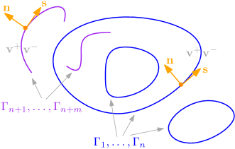
Figure 1. Illustration of the closed curves $\Gamma_{1},\dots,\Gamma_{n}$ and the open curves $\Gamma_{n+1},\dots,\Gamma_{n+m}$, and the definitions of $\mathbf{n}$, $\mathbf{s}$, $\mathbf{v}^{+}$ and $\mathbf{v}^{-}$.

In the following lemma, we derive the equation that the Birkhoff-Rott integral satisfies for a stationary/rotating vortex sheet.

Lemma 2.1.

Assume $\omega(\cdot,t)=\omega_{0}(R_{\Omega t}x)$ is a stationary/uniformly-rotating vortex sheet with angular velocity $\Omega\in\mathbb{R}$, and $\omega_{0}$ is concentrated on $\cup_{i=1}^{n+m}\Gamma_{i}$, with $z_{i}$ and $\gamma_{i}$ defined as above. Then the Birkhoff-Rott integral $BR$ (2.4) and the strength $\gamma_{i}$ satisfy the following two equations:

$$(BR-\Omega x^{\perp})\cdot\mathbf{n}=\mathbf{v}^{+}\cdot\mathbf{n}=\mathbf{v}^{-}\cdot\mathbf{n}=0\quad\text{ on }\Gamma,$$ (2.6)

and

$$(BR(z_{i}(\alpha))-\Omega z_{i}^{\perp}(\alpha))\cdot\mathbf{s}(z_{i}(\alpha))\,\gamma_{i}(\alpha)=\begin{cases}C_{i}&\text{ on }S_{i}\text{ for }i=1,\dots,n,\\ 0&\text{ on }S_{i}\text{ for }i=n+1,\dots,n+m.\end{cases}$$ (2.7)

In particular, the above two equations imply that $BR(z_{i}(\alpha))-\Omega z_{i}^{\perp}(\alpha)\equiv\mathbf{0}$ for $i=n+1,\dots,n+m$.

Proof.

By definition of the stationary/uniformly-rotating solutions, $\omega_{0}$ is a stationary vortex sheet in the rotating frame with angular velocity $\Omega$. In this rotating frame, an extra velocity $-\Omega z_{i}^{\perp}$ should be added to the right hand side of (1.4). Therefore the evolution equations (1.4)–(1.5) become the following in the rotating frame (where we also use (2.4)):

$$\partial_{t}z_{i}(\alpha,t) =BR(z_{i}(\alpha,t))-\Omega z_{i}^{\perp}(\alpha,t)+c_{i}(\alpha,t)\partial_{\alpha}z_{i}(\alpha,t)$$ (2.8)

$$\partial_{t}\varpi_{i}(\alpha,t) =\partial_{\alpha}(c_{i}(\alpha,t)\varpi_{i}(\alpha,t)),$$ (2.9)

where the term $c_{i}(\alpha,t)$ accounts for the reparametrization freedom of the curves. Since $\omega_{0}$ is stationary in the rotating frame, $z_{i}(\cdot,t)$ parametrizes the same curve as $z_{i}(\cdot,0)$. Therefore $\partial_{t}z_{i}(\alpha,t)$ is tangent to the curve $\Gamma_{i}$, and multiplying $\mathbf{n}(z_{i}(\alpha,t))$ to (2.8) gives

$$0=\partial_{t}z_{i}(\alpha,t)\cdot\mathbf{n}(z_{i}(\alpha,t))=(BR(z_{i}(\alpha,t))-\Omega z_{i}^{\perp}(\alpha,t))\cdot\mathbf{n}(z_{i}(\alpha,t)),$$ (2.10)

where we use that $\mathbf{n}(z_{i}(\alpha,t))\cdot\partial_{\alpha}z_{i}(\alpha,t)=0$. This proves (2.6).

Now we prove (2.7). Towards this end, let us choose

$$c_{i}(\alpha,t):=-\frac{(BR(z_{i}(\alpha,t))-\Omega z_{i}^{\perp}(\alpha,t))\cdot\mathbf{s}(z_{i}(\alpha,t))}{|\partial_{\alpha}z_{i}(\alpha,t)|},$$

so that multiplying $\mathbf{s}(z_{i}(\alpha,t))$ to (2.8) gives $\partial_{t}z_{i}(\alpha,t)\cdot\mathbf{s}(z_{i}(\alpha,t))=0$, and combining it with (2.10) gives $\partial_{t}z_{i}(\alpha,t)=0.$ In other words, with such choice of $c_{i}$, the parametrization $z_{i}(\alpha,t)$ remains fixed in time. Since $\omega_{0}$ is stationary in the rotating frame, we know that with a fixed parametrization $z_{i}(\alpha,t)=z_{i}(\alpha,0)$, the strength $\varpi_{i}(\alpha,t)$ must also remain invariant in time. Thus (2.9) becomes

$$c_{i}(\alpha,t)\varpi_{i}(\alpha,t)\equiv C_{i}.$$

Plugging the definition of $c_{i}$ into the equation above and using the fact that $z_{i}$ is invariant in $t$, we have

$$\frac{(BR(z_{i}(\alpha))-\Omega z_{i}^{\perp}(\alpha))\cdot\mathbf{s}(z_{i}(\alpha))\varpi_{i}(\alpha)}{|\partial_{\alpha}z_{i}(\alpha)|}\equiv-C_{i}\quad\text{ for all }\alpha\in S_{i},$$

and finally the relationship between $\gamma_{i}$ and $\varpi_{i}$ in (2.3) yields (2.7) for $i=1,\dots,n$.

And for the open curves $i=n+1,\dots,n+m$, note that we do not have any reparametrization freedom at the two endpoints $\alpha=0,1$, therefore the endpoint velocity $BR(z_{i}(0,t))-\Omega z_{i}^{\perp}(0,t)$ must be 0 to ensure that $\omega_{0}$ is stationary in the rotating frame. This immediately leads to $C_{i}=0$ for $i=n+1,\dots,n+m$, finishing the proof of (2.7). ∎

3. Approximation by a thin vortex layer

Our aim in this section is to desingularize the vortex sheet $\omega_{0}$. Namely, for $0<\epsilon\ll 1$, we will construct a vorticity $\omega^{\epsilon}\in L^{\infty}(\mathbb{R}^{2})\cap L^{1}(\mathbb{R}^{2})$ that only takes values $0$ and $\epsilon^{-1}$, and is supported in an $O(\epsilon)$ neighborhood of $\Gamma$, such that $\omega^{\epsilon}$ weakly converges to $\omega_{0}$ as $\epsilon\to 0^{+}$.

For each $i=1,\dots,n+m$, we will describe a neighborhood of $\Gamma_{i}$ using the following change of coordinates: let $R^{\epsilon}_{i}:S_{i}\times\mathbb{R}\to\mathbb{R}^{2}$ be given by

$$R^{\epsilon}_{i}(\alpha,\eta):=z_{i}(\alpha)+\epsilon\gamma_{i}(\alpha)\mathbf{n}(z_{i}(\alpha))\eta,$$ (3.1)

and let

$$D^{\epsilon}_{i}:=\left\{R^{\epsilon}_{i}(\alpha,\eta):\alpha\in S_{i}^{\circ},\eta\in(-1,0)\right\}.$$

Note that each $D^{\epsilon}_{i}$ is a connected open set, and for all $\epsilon>0$ sufficiently small, the sets $(D^{\epsilon}_{i})_{i=1}^{n+m}$ are disjoint. For $i=1,\dots,n$, the domains $D_{i}^{\epsilon}$ are doubly-connected with smooth boundary, and its inner boundary coincides with $\Gamma_{i}$; see the left of Figure 2 for an illustration. And for $i=n+1,\dots,n+m$, the domains $D_{i}^{\epsilon}$ are simply-connected, and its boundary is smooth except at at most two points; see the right of Figure 2 for an illustration.

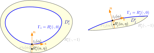
Figure 2. Illustration of the definitions of $R_{i}^{\epsilon}$ and $D_{i}^{\epsilon}$ for a closed curve (left) and an open curve (right).

In addition, for $\epsilon>0$ that is sufficiently small, one can check that $R^{\epsilon}_{i}:S_{i}^{\circ}\times(-1,0)\to D_{i}^{\epsilon}$ is a diffeomorphism. Since $\gamma_{i}\in C^{1}(S_{i})$ and $z_{i}\in C^{2}(S_{i})$, we only need to show $R^{\epsilon}_{i}:S_{i}^{\circ}\times(-1,0)\to D_{i}^{\epsilon}$ is injective. Below we prove this fact in a stronger quantitative version, which will be used later.

Lemma 3.1.

For any $i=1,\dots,n+m$, assume $\Gamma_{i}$ and $\gamma_{i}$ satisfy (H1)–(H2). Then the map $R^{\epsilon}_{i}:S_{i}^{\circ}\times(-1,0)\to D^{\epsilon}_{i}$ given by (3.1) is injective. In addition, there exist some $c_{0},\epsilon_{0}>0$ depending on $\|z_{i}\|_{C^{2}(S_{i})},$ $\rVert\gamma_{i}\rVert_{L^{\infty}(S_{i})}$ and $F_{\Gamma}$, such that for all $\epsilon\in(0,\epsilon_{0})$ we have

$$|R^{\epsilon}_{i}(\alpha^{\prime},\eta^{\prime})-R^{\epsilon}_{i}(\alpha,\eta)|\geq c_{0}\big{(}|\alpha^{\prime}-\alpha|+\epsilon|\gamma_{i}(\alpha)\eta-\gamma_{i}(\alpha^{\prime})\eta^{\prime}|\big{)},$$ (3.2)

for all $\alpha,\alpha^{\prime}\in S_{i}^{\circ},~{}\eta,\eta^{\prime}\in(-1,0)$.

Proof.

To begin with, note that (3.2) immediately implies that $R^{\epsilon}_{i}:S_{i}^{\circ}\times(-1,0)\to D^{\epsilon}_{i}$ is injective, where we used the positivity assumption $\gamma_{i}>0$ in $S_{i}^{\circ}$ in (H2). Thus it suffices to prove (3.2). Throughout the proof, we fix any $i\in\{1,\dots,n+m\}$, and we will omit the subscript $i$ for notational simplicity. Using the definition (3.1), let us break $R^{\epsilon}(\alpha^{\prime},\eta^{\prime})-R^{\epsilon}(\alpha,\eta)$ into

$$R^{\epsilon}(\alpha^{\prime},\eta^{\prime})-R^{\epsilon}(\alpha,\eta)=\underbrace{z(\alpha^{\prime})-z(\alpha)}_{=:T_{1}}+\underbrace{\epsilon\left(\gamma(\alpha^{\prime})\eta^{\prime}-\gamma(\alpha)\eta\right)\mathbf{n}(z(\alpha^{\prime}))}_{=:T_{2}}+\underbrace{\epsilon\gamma(\alpha)\eta\left(\mathbf{n}(z(\alpha^{\prime}))-\mathbf{n}(z(\alpha))\right)}_{=:T_{3}}.$$ (3.3)

For $T_{1}$ and $T_{3}$, we have

$$\begin{split}\left|T_{1}-z^{\prime}(\alpha^{\prime})(\alpha^{\prime}-\alpha)\right|&\leq\rVert z\rVert_{C^{2}(S)}|\alpha-\alpha^{\prime}|^{2},\\ \left|T_{3}\right|&\leq\epsilon\gamma(\alpha)\rVert z\rVert_{C^{2}(S)}|\alpha-\alpha^{\prime}|.\end{split}$$ (3.4)

Also, using that $z^{\prime}(\alpha^{\prime})=L\mathbf{s}(z(\alpha^{\prime}))$ is perpendicular to $\mathbf{n}(z(\alpha^{\prime}))$, we have

$$\begin{split}|z^{\prime}(\alpha^{\prime})(\alpha^{\prime}-\alpha)+T_{2}|&=\left|L(\alpha^{\prime}-\alpha)\mathbf{s}(z(\alpha^{\prime}))+\epsilon\left(\gamma(\alpha^{\prime})\eta^{\prime}-\gamma(\alpha)\eta\right)\mathbf{n}(z(\alpha^{\prime}))\right|\\ &\geq\frac{1}{2}L|\alpha^{\prime}-\alpha|+\frac{1}{2}\epsilon\left|\gamma(\alpha^{\prime})\eta^{\prime}-\gamma(\alpha)\eta\right|,\end{split}$$

where we use that $\sqrt{x^{2}+y^{2}}\geq\frac{1}{2}(|x|+|y|)$. Combining this with (3.4) gives

$$|T_{1}+T_{2}+T_{3}| \geq|\alpha-\alpha^{\prime}|\left(\frac{L}{2}-\rVert z\rVert_{C^{2}(S)}\left(|\alpha-\alpha^{\prime}|+\epsilon\gamma(\alpha)\right)\right)+\frac{1}{2}\epsilon|\gamma(\alpha^{\prime})\eta^{\prime}-\gamma(\alpha)\eta|,$$

thus

$$|R^{\epsilon}(\alpha^{\prime},\eta^{\prime})-R^{\epsilon}(\alpha,\eta)|\geq\frac{L}{4}|\alpha-\alpha^{\prime}|+\frac{1}{2}\epsilon|\gamma(\alpha^{\prime})\eta^{\prime}-\gamma(\alpha)\eta|$$ (3.5)

for all $0<\epsilon<L(8\rVert z\rVert_{C^{2}}\rVert\gamma\rVert_{L^{\infty}})^{-1}$ and $|\alpha-\alpha^{\prime}|\leq\frac{L}{8\rVert z\rVert_{C^{2}}}$.

For $|\alpha-\alpha^{\prime}|>\frac{L}{8\rVert z\rVert_{C^{2}}}$, recall that the definition of $F_{\Gamma}$ in (2.2) gives $|z(\alpha^{\prime})-z(\alpha)|\geq F_{\Gamma}^{-1}|\alpha^{\prime}-\alpha|$. Thus a crude estimate gives

$$|R^{\epsilon}(\alpha^{\prime},\eta^{\prime})-R^{\epsilon}(\alpha,\eta)|\geq|z(\alpha^{\prime})-z(\alpha)|-2\epsilon\|\gamma\|_{L^{\infty}(S)}\geq\frac{1}{2F_{\Gamma}}|\alpha^{\prime}-\alpha|+\epsilon|\gamma(\alpha^{\prime})\eta^{\prime}-\gamma(\alpha)\eta|$$ (3.6)

for $0<\epsilon<L(64F_{\Gamma}\|z\|_{C^{2}}\|\gamma\|_{L^{\infty}})^{-1}$. (Note that for such $\epsilon$ we have $4\epsilon\|\gamma\|_{L^{\infty}}\leq\frac{1}{2F_{\Gamma}}|\alpha^{\prime}-\alpha|$ due to our assumption that $|\alpha-\alpha^{\prime}|>\frac{L}{8\rVert z\rVert_{C^{2}}}$).

Finally, combining (3.5) and (3.6), it follows that (3.2) holds for $c_{0}=\min\{\frac{L}{4},\frac{1}{2F_{\Gamma}},\frac{1}{2}\}$ and $\epsilon_{0}=\min\{L(8\rVert z\rVert_{C^{2}}\rVert\gamma\rVert_{L^{\infty}})^{-1},L(64F_{\Gamma}\|z\|_{C^{2}}\|\gamma\|_{L^{\infty}})^{-1}\}$. This finishes the proof. ∎

In the next lemma we compute the partial derivatives and Jacobian of $R^{\epsilon}_{i}(\alpha,\eta)$, which will be useful later.

Lemma 3.2.

For any $i=1,\dots,n+m$, let $z_{i}$ be a constant-speed parameterization of the curve $\Gamma_{i}$ (with length $L_{i}$), and let $R^{\epsilon}_{i}$ be given by (3.1). Then its partial derivatives are

$$\begin{split}\partial_{\alpha}R^{\epsilon}_{i}(\alpha,\eta)&=z_{i}^{\prime}(\alpha)+\epsilon\left(\gamma_{i}^{\prime}(\alpha)\frac{z_{i}^{\prime}(\alpha)^{\perp}}{L_{i}}\eta+\gamma_{i}(\alpha)\frac{z_{i}^{\prime\prime}(\alpha)^{\perp}}{L_{i}}\eta\right),\\ \partial_{\eta}R^{\epsilon}_{i}(\alpha,\eta)&=\epsilon\gamma_{i}(\alpha)\frac{z_{i}^{\prime}(\alpha)^{\perp}}{L_{i}}.\end{split}$$ (3.7)

Moreover, its Jacobian is given by

$$\begin{split}\det(\nabla_{\alpha,\eta}R^{\epsilon}_{i})&=\epsilon L_{i}\gamma_{i}(\alpha)-\epsilon^{2}L_{i}\gamma_{i}^{2}(\alpha)\kappa_{i}(\alpha)\eta,\end{split}$$ (3.8)

where $\kappa_{i}(\alpha)$ denotes the signed curvature of $\Gamma_{i}$ at $z_{i}(\alpha)$.

Proof.

Since $z_{i}$ is the constant-speed parameterization of $\Gamma_{i}$ (which has length $L_{i}$), we have $|z_{i}^{\prime}|\equiv L_{i}$ and $\mathbf{n}(z_{i}(\alpha))=z_{i}^{\prime}(\alpha)^{\perp}/L_{i}$. Taking the $\alpha$ and $\eta$ partial derivatives of (3.1) directly yields (3.7).

Putting the two partial derivatives into columns of a $2\times 2$ matrix and computing the determinant, we have

$$\begin{split}\det(\nabla_{\alpha,\eta}R_{i}^{\epsilon})&=\epsilon\gamma_{i}(\alpha)\frac{|z_{i}^{\prime}(\alpha)|^{2}}{L_{i}}+\epsilon^{2}\gamma_{i}^{2}(\alpha)\frac{z_{i}^{\prime\prime}(\alpha)^{\perp}\cdot z_{i}^{\prime}(\alpha)}{L_{i}^{2}}\eta\\ &=\epsilon L_{i}\gamma_{i}(\alpha)-\epsilon^{2}L_{i}\gamma_{i}^{2}(\alpha)\kappa_{i}(\alpha)\eta,\end{split}$$

where in the second equality we used that $z_{i}^{\prime\prime}(\alpha)=\kappa_{i}(\alpha)\mathbf{n}(z_{i}(\alpha))L_{i}^{2}$ (recall that $z_{i}$ has constant speed $L_{i}$). This finishes the proof. ∎

Remark 3.3.

We point out that for each $i=1,\dots,n+m$, the determinant formula (3.8) immediately gives the following approximation of $|D^{\epsilon}_{i}|$, which will be helpful in the proofs later:

$$\frac{|D^{\epsilon}_{i}|}{\epsilon}=\frac{1}{\epsilon}\int_{D^{\epsilon}_{i}}1dx=\frac{1}{\epsilon}\int_{S_{i}}\int_{-1}^{0}\det(\nabla_{\alpha,\eta}R^{\epsilon}_{i}(\alpha,\eta))\,d\eta d\alpha=L_{i}\int_{S_{i}}\gamma_{i}(\alpha)d\alpha+O(\epsilon),$$ (3.9)

where the $O(\epsilon)$ error term has its absolute value bounded by $C\epsilon$, with $C$ only depending on $\|z_{i}\|_{C^{2}(S_{i})}$ and $\|\gamma_{i}\|_{L^{\infty}(S_{i})}$.

Finally, let $D^{\epsilon}:=\cup_{i=1}^{n+m}D_{i}^{\epsilon}$, and $\omega^{\epsilon}:\mathbb{R}^{2}\to\mathbb{R}$ is defined as

$$\omega^{\epsilon}(x):=\epsilon^{-1}1_{D^{\epsilon}}(x)=\epsilon^{-1}\sum_{i=1}^{n+m}1_{D_{i}^{\epsilon}}(x),$$

and let

$$\mathbf{v}^{\epsilon}=\nabla^{\perp}(\omega^{\epsilon}*\mathcal{N})$$ (3.10)

be the velocity field generated by $\omega^{\epsilon}$.

In the next lemma we aim to obtain some fine estimate of $\mathbf{v}^{\epsilon}$ in the thin vortex layer $D^{\epsilon}$. Our goal is to show that along each cross section of the thin layer (i.e. fix $i$ and $\alpha$, and let $\eta$ vary in $[-1,0]$), the function $\eta\mapsto\mathbf{v}^{\epsilon}(R_{i}^{\epsilon}(\alpha,\eta))$ is almost a linear function in $\eta$, with the endpoint values (at $\eta=-1$ and $0$) being almost $\mathbf{v}^{-}(z_{i}(\alpha))$ and $\mathbf{v}^{+}(z_{i}(\alpha))$ respectively.

Lemma 3.4.

For $i=1,\dots,n+m$, assume $\Gamma_{i}$ and $\gamma_{i}$ satisfy (H1)–(H3). Let

$$g_{i}(\alpha,\eta):=BR(z_{i}(\alpha))-\Big{(}\eta+\frac{1}{2}\Big{)}[\mathbf{v}](z_{i}(\alpha))\quad\text{ for }\alpha\in S_{i},$$

and note that $g_{i}(\alpha,0)=\mathbf{v}^{+}(z_{i}(\alpha))$ and $g_{i}(\alpha,-1)=\mathbf{v}^{-}(z_{i}(\alpha))$ (see Figure 3 for an illustration of $g_{i}(\alpha,\eta)$). Then for all sufficiently small $\epsilon>0$, for all $i=1,\dots,n+m$ we have

$$|\mathbf{v}^{\epsilon}(R_{i}^{\epsilon}(\alpha,\eta))-g_{i}(\alpha,\eta)|\leq C\epsilon^{b}|\log\epsilon|\quad\text{ for all }\alpha\in S_{i},\eta\in[-1,0],$$ (3.11)

where $b\in(0,1)$ is as in (H2), and $C$ depends on $b$, $\max_{i}\|z_{i}\|_{C^{2}(S_{i})}$, $\max_{i}\|\gamma_{i}\|_{C^{b}(S_{i})}$, $d_{\Gamma}$ and $F_{\Gamma}$.

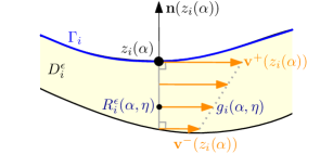
Figure 3. Illustration of the definition of $g_{i}(\alpha,\cdot)$ (the orange arrows).

Proof.

Let $i$ be any fixed index in $1,\dots,n+m$. We begin with breaking $\mathbf{v}^{\epsilon}$ into contributions from different components $\{D_{k}^{\epsilon}\}_{k=1}^{n+m}$, namely

$$\mathbf{v}^{\epsilon}(x)=\sum_{k=1}^{n+m}\mathbf{v}_{k}^{\epsilon}(x):=\sum_{k=1}^{n+m}\epsilon^{-1}\int_{D_{i}^{\epsilon}}K_{2}(x-y)dy,$$

where the kernel $K_{2}$ is given by (2.5). Similarly, we can break $BR(z_{i}(\alpha))$ into $\displaystyle BR(z_{i}(\alpha))=\sum_{k=1}^{n+m}BR_{k}(z_{i}(\alpha)),$ where $BR_{k}$ is the contribution from the $k$-th integral in (2.4), and note that the PV symbol is only needed for $k=i$.

$\bullet$ Estimates for $k\neq i$ terms. For any $k\neq i$, we aim to show that

$$|\mathbf{v}_{k}^{\epsilon}(R_{i}^{\epsilon}(\alpha,\eta))-BR_{k}(z_{i}(\alpha))|\leq C\epsilon,$$ (3.12)

where $C$ depends on $d_{\Gamma},\max_{k}\|z_{k}\|_{C^{2}}$ and $\max_{k}\|\gamma_{k}\|_{L^{\infty}}$. Applying a change of variable $y=R_{k}^{\epsilon}(\alpha^{\prime},\eta^{\prime})$, we can rewrite $\mathbf{v}_{k}^{\epsilon}$ as

$$\begin{split}\mathbf{v}_{k}^{\epsilon}(R_{i}^{\epsilon}(\alpha,\eta))&=\epsilon^{-1}\int_{D_{k}^{\epsilon}}K_{2}(R_{i}^{\epsilon}(\alpha,\eta)-y)\,dy\\ &=\int_{S_{k}}\int_{-1}^{0}\underbrace{K_{2}(R_{i}^{\epsilon}(\alpha,\eta)-R_{k}^{\epsilon}(\alpha^{\prime},\eta^{\prime}))}_{=:T_{1}}\underbrace{\epsilon^{-1}\det(\nabla_{\alpha^{\prime},\eta^{\prime}}R_{k}^{\epsilon}(\alpha^{\prime},\eta^{\prime}))}_{=:T_{2}}\,d\eta^{\prime}d\alpha^{\prime}.\end{split}$$ (3.13)

Using the facts that $R_{i}^{\epsilon}(\alpha,\eta)-R_{k}^{\epsilon}(\alpha^{\prime},\eta^{\prime})=z_{i}(\alpha)-z_{k}(\alpha^{\prime})+O(\epsilon)$ as well as $|z_{i}(\alpha)-z_{k}(\alpha^{\prime})|\geq d_{\Gamma}>0$ (recall that $d_{\Gamma}$ is as given in (2.1)), for all sufficiently small $\epsilon>0$ we have $T_{1}=K_{2}(z_{i}(\alpha)-z_{k}(\alpha^{\prime}))+O(\epsilon).$ For $T_{2}$, the explicit formula (3.8) for the determinant gives $T_{2}=L_{k}\gamma_{k}(\alpha^{\prime})+O(\epsilon).$ Plugging these into the above integral yields

$$\mathbf{v}_{k}^{\epsilon}(R_{i}^{\epsilon}(\alpha,\eta))=\int_{S_{k}}K_{2}(z_{i}(\alpha)-z_{k}(\alpha^{\prime}))L_{k}\gamma_{k}(\alpha^{\prime})\,d\alpha^{\prime}+O(\epsilon)=BR_{k}(z_{i}(\alpha))+O(\epsilon),$$

finishing the proof of (3.12).

$\bullet$ Estimates for the $k=i$ term. It will be more involved to control the $k=i$ term, and our goal is to show that

$$\left|\mathbf{v}_{i}^{\epsilon}(R_{i}^{\epsilon}(\alpha,\eta))-BR_{i}(z_{i}(\alpha))+\Big{(}\eta+\frac{1}{2}\Big{)}[\mathbf{v}](z_{i}(\alpha))\right|\leq C\epsilon^{b}|\log\epsilon|.$$ (3.14)

To begin with, we again rewrite $\mathbf{v}_{i}^{\epsilon}$ as in (3.13) with $k=i$, and plug in the formula (3.8) for the determinant. This leads to

$$\begin{split}\mathbf{v}_{i}^{\epsilon}(R_{i}^{\epsilon}(\alpha,\eta))&=\int_{S_{k}}\int_{-1}^{0}K_{2}(R_{i}^{\epsilon}(\alpha,\eta)-R_{i}^{\epsilon}(\alpha^{\prime},\eta^{\prime}))\left(L_{i}\gamma_{i}(\alpha^{\prime})-\epsilon L_{i}\gamma_{i}^{2}(\alpha^{\prime})\kappa_{i}(\alpha^{\prime})\eta^{\prime}\right)\,d\eta^{\prime}d\alpha^{\prime}\\ &=:I_{1}+I_{2},\end{split}$$

where $I_{1},I_{2}$ are the contributions from the two terms in the last parenthesis respectively. Let us control $I_{2}$ first, and we claim that

$$|I_{2}|\leq C\epsilon|\log\epsilon|.$$ (3.15)

Using (3.2) of Lemma 3.1 and the fact that $|K_{2}(x)|\leq|x|^{-1}$, we can bound $I_{2}$ as

$$\begin{split}|I_{2}|&=\left|\int_{S_{k}}\int_{-1}^{0}K_{2}(R_{i}^{\epsilon}(\alpha,\eta)-R_{i}^{\epsilon}(\alpha^{\prime},\eta^{\prime}))\,\epsilon L_{i}\gamma_{i}^{2}(\alpha^{\prime})\kappa_{i}(\alpha^{\prime})\eta^{\prime}\,d\eta^{\prime}d\alpha^{\prime}\right|\\ &\leq C\epsilon\int_{S_{k}}\int_{-1}^{0}\frac{\gamma_{i}(\alpha^{\prime})}{|\alpha^{\prime}-\alpha|+\epsilon|\gamma_{i}(\alpha^{\prime})\eta^{\prime}-\gamma_{i}(\alpha)\eta|}\,d\eta^{\prime}d\alpha^{\prime}\\ &\leq C\epsilon\int_{S_{k}}\int_{-\|\gamma_{i}\|_{\infty}}^{\|\gamma_{i}\|_{\infty}}\frac{1}{|\alpha^{\prime}-\alpha|+\epsilon|\theta^{\prime}|}\,d\theta^{\prime}d\alpha^{\prime}\quad(\theta^{\prime}:=\gamma_{i}(\alpha^{\prime})\eta^{\prime}-\gamma_{i}(\alpha)\eta)\\ &\leq C\epsilon\int_{-1/\epsilon}^{1/\epsilon}\int_{-\|\gamma_{i}\|_{\infty}}^{\|\gamma_{i}\|_{\infty}}\frac{1}{|\beta^{\prime}|+|\theta^{\prime}|}\,d\theta^{\prime}d\beta^{\prime}\quad(\beta^{\prime}:=\epsilon^{-1}(\alpha^{\prime}-\alpha))\\ &\leq C\epsilon|\log\epsilon|\end{split}$$ (3.16)

where $C$ depends on $\|z_{i}\|_{C^{2}}$ and $\|\gamma_{i}\|_{L^{\infty}}$.

In the rest of the proof we focus on estimating $I_{1}=\displaystyle\int_{S_{k}}\int_{-1}^{0}K_{2}(R_{i}^{\epsilon}(\alpha,\eta)-R_{i}^{\epsilon}(\alpha^{\prime},\eta^{\prime}))L_{i}\gamma_{i}(\alpha^{\prime})\,d\eta^{\prime}d\alpha^{\prime}.$ For $t\in[0,1]$, let us define

$$f(\alpha,\alpha^{\prime},\eta,\eta^{\prime};t):=R_{i}^{\epsilon}(\alpha,\eta-t\eta^{\prime})-R_{i}^{\epsilon}(\alpha^{\prime},\eta^{\prime}-t\eta^{\prime}),$$

$$J(t):=\int_{S_{k}}\int_{-1}^{0}K_{2}(f(\alpha,\alpha^{\prime},\eta,\eta^{\prime};t))L_{i}\gamma_{i}(\alpha^{\prime})\,d\eta^{\prime}d\alpha^{\prime}.$$ (3.17)

Note that in the definition of $f$, the argument $\eta-t\eta^{\prime}$ of $R_{i}^{\epsilon}$ belongs to $[-1,1]$, instead of $[-1,0]$ as in the original definition of (3.1). Here $R_{i}^{\epsilon}(\alpha,\eta-t\eta^{\prime})$ is defined as in the formula (3.1), even though it might not belong to $D^{\epsilon}_{i}$. Clearly, $J(0)=I_{1}$. The motivation for us to define such $f$ and $J(t)$ is that at $t=1$, we have

$$\begin{split}J(1)&=\int_{S_{k}}\int_{-1}^{0}K_{2}(R_{i}^{\epsilon}(\alpha,\eta-\eta^{\prime})-z_{i}(\alpha^{\prime}))L_{i}\gamma_{i}(\alpha^{\prime})\,d\eta^{\prime}d\alpha^{\prime}=\int_{-1}^{0}\mathbf{v}_{i}(R_{i}^{\epsilon}(\alpha,\eta-\eta^{\prime}))\,d\eta^{\prime},\end{split}$$ (3.18)

where $\mathbf{v}_{i}$ is the velocity field generated by the sheet $\Gamma_{i}$. Recall that $\mathbf{v}_{i}$ has a jump across $\Gamma_{i}$, where we denote its limits on two sides by $\mathbf{v}_{i}^{\pm}$. Using Lemma 3.5, which we will prove momentarily, we have

$$\mathbf{v}_{i}(R_{i}^{\epsilon}(\alpha,\eta-\eta^{\prime}))=\begin{cases}\mathbf{v}_{i}^{+}(z_{i}(\alpha))+O(\epsilon^{b}|\log\epsilon|)&\text{ if }\eta-\eta^{\prime}\in(0,2),\\ \mathbf{v}_{i}^{-}(z_{i}(\alpha))+O(\epsilon^{b}|\log\epsilon|)&\text{ if }\eta-\eta^{\prime}\in(-2,0).\end{cases}$$ (3.19)

We can then split the integration domain on the right hand side of (3.18) into $\eta^{\prime}\in(-1,\eta)$ and $\eta^{\prime}\in(\eta,0)$, and use (3.19) to approximate the integrand in each interval. This gives

$$\begin{split}J(1)&=(\eta+1)\mathbf{v}_{i}^{+}(z_{i}(\alpha))-\eta\mathbf{v}_{i}^{-}(z_{i}(\alpha))+O(\epsilon^{b}|\log\epsilon|)\\ &=BR_{i}(z_{i}(\alpha))-\Big{(}\eta+\frac{1}{2}\Big{)}[\mathbf{v}](z_{i}(\alpha))+O(\epsilon^{b}|\log\epsilon|),\end{split}$$ (3.20)

where in the last step we used that $[\mathbf{v}](z_{i}(\alpha))=[\mathbf{v}_{i}](z_{i}(\alpha))$, since all other $\mathbf{v}_{k}$ with $k\neq i$ are continuous across $\Gamma_{i}$.

Finally, it remains to control $|J(0)-J(1)|$. Note that by (3.2), we have

$$f(\alpha,\alpha^{\prime},\eta,\eta^{\prime};t)\geq c_{0}\big{(}|\alpha-\alpha^{\prime}|+\epsilon|\gamma_{i}(\alpha^{\prime})\eta^{\prime}-\gamma_{i}(\alpha)\eta|\big{)}.$$

In addition, we have

$$\left|\frac{\partial}{\partial t}f(\alpha,\alpha^{\prime},\eta,\eta^{\prime};t)\right|=\left|\epsilon\big{(}\gamma_{i}(\alpha)\mathbf{n}(z_{i}(\alpha))-\gamma_{i}(\alpha^{\prime})\mathbf{n}(z_{i}(\alpha^{\prime}))\big{)}\eta^{\prime}\right|\leq C\epsilon|\alpha-\alpha^{\prime}|^{b},$$

where the last inequality follows from (H2) and the fact that $\mathbf{n}(z_{i}(\alpha))\in C^{1}(S_{i})$. Therefore, for any $t\in(0,1)$, taking the $t$ derivative of (3.17) and using that $|\nabla K_{2}(x)|\leq|x|^{-2}$, we have

$$\begin{split}|J^{\prime}(t)|&\leq C\int_{S_{k}}\int_{-1}^{0}\frac{\epsilon|\alpha-\alpha^{\prime}|^{b}\gamma_{i}(\alpha^{\prime})}{\big{(}|\alpha-\alpha^{\prime}|+\epsilon|\gamma_{i}(\alpha^{\prime})\eta^{\prime}-\gamma_{i}(\alpha)\eta|\big{)}^{2}}d\eta^{\prime}d\alpha^{\prime}\\ &\leq C\epsilon\int_{S_{k}}\int_{-1}^{0}\frac{\gamma_{i}(\alpha^{\prime})}{|\alpha-\alpha^{\prime}|^{1-b}\left(|\alpha-\alpha^{\prime}|+\epsilon|\gamma_{i}(\alpha^{\prime})\eta^{\prime}-\gamma_{i}(\alpha)\eta|\right)}d\eta^{\prime}d\alpha^{\prime}\\ &\leq C\epsilon^{b}\int_{-1/\epsilon}^{1/\epsilon}\int_{-\|\gamma_{i}\|_{\infty}}^{\|\gamma_{i}\|_{\infty}}\frac{1}{|\beta^{\prime}|^{1-b}(|\beta^{\prime}|+|\theta^{\prime}|)}\,d\theta^{\prime}d\beta^{\prime}\quad(\theta^{\prime}:=\gamma_{i}(\alpha^{\prime})\eta^{\prime}-\gamma_{i}(\alpha)\eta,\,\beta^{\prime}:=\epsilon^{-1}(\alpha^{\prime}-\alpha))\\ &\leq C\epsilon^{b}\int_{-1/\epsilon}^{1/\epsilon}|\beta^{\prime}|^{b-1}\log\left(1+\frac{\|\gamma_{i}\|_{L^{\infty}}}{|\beta^{\prime}|}\right)d\beta^{\prime}\\ &\leq C\epsilon^{b},\end{split}$$

where $C$ depends on $b$, $\|\gamma_{i}\|_{C^{b}(S_{i})}$, $\|z_{i}\|_{C^{2}(S_{i})}$ and $F_{\Gamma}$. This leads to

$$|J(1)-I_{1}|=|J(1)-J(0)|\leq C\epsilon^{b}|\log\epsilon|.$$

Finally, combining this with (3.20) and (3.15) yields (3.14), finishing the proof of the $k=i$ case. We can then conclude the proof by taking the sum of this estimate with all the $k\neq i$ estimates in (3.12). ∎

The following lemma proves (3.19). Let $\mathbf{v}_{i}$ be the velocity field generated by the sheet $\Gamma_{i}$, which is smooth in $\mathbb{R}^{2}\setminus\Gamma_{i}$, and has a discontinuity across $\Gamma_{i}$. It is known that $\mathbf{v}_{i}$ converges to $\mathbf{v}_{i}^{\pm}$ respectively on the two sides of $\Gamma_{i}$ [24]. However, we were unable to find a quantitative convergence rate (in terms of the distance from the point to $\Gamma_{i}$) in the literature, especially under the assumption that $\gamma_{i}$ is only in $C^{b}(S_{i})$ for the open curves. Below we prove such an estimate.

Lemma 3.5.

For $i=1,\ldots,n+m$, let $\mathbf{v}_{i}$ be the velocity field generated by the sheet $\Gamma_{i}$, given by

$$\mathbf{v}_{i}(x):=\int_{S_{i}}K_{2}(x-z_{i}(\alpha^{\prime}))\,\gamma_{i}(\alpha^{\prime})|z_{i}^{\prime}(\alpha^{\prime})|\,d\alpha^{\prime}\quad\text{ for }x\in\mathbb{R}^{2}\setminus\Gamma_{i}.$$

Then there exist constants $C,\epsilon_{0}>0$ depending on on $b$ (as in (H2)), $\|z_{i}\|_{C^{2}(S_{i})}$, $\|\gamma_{i}\|_{C^{b}(S_{i})}$ and $F_{\Gamma}$, such that for all $\epsilon\in(0,\epsilon_{0})$ and $\eta\in(-2,2)$ we have

$$\left|\mathbf{v}_{i}(R^{\epsilon}_{i}(\alpha,\eta))-\mathbf{v}_{i}^{+}(z_{i}(\alpha))\right|\leq C\epsilon^{b}|\log\epsilon|\quad\text{ if }\eta\in(0,2),$$ (3.21)

$$\left|\mathbf{v}_{i}(R^{\epsilon}_{i}(\alpha,\eta))-\mathbf{v}_{i}^{-}(z_{i}(\alpha))\right|\leq C\epsilon^{b}|\log\epsilon|\quad\text{ if }\eta\in(-2,0),$$ (3.22)

where

$$\mathbf{v}_{i}^{+}=BR_{i}(z_{i}(\alpha))+\frac{\mathbf{n}(z_{i}(\alpha))^{\perp}\gamma_{i}(\alpha)}{2},\quad\mathbf{v}_{i}^{-}=BR_{i}(z_{i}(\alpha))-\frac{\mathbf{n}(z_{i}(\alpha))^{\perp}\gamma_{i}(\alpha)}{2},$$

and $BR_{i}$ is the contribution from the $i$-th integral in (2.4).

Proof.

We will show (3.21) only since (3.22) can be treated in the same way. From the definition of $R^{\epsilon}_{i}$ in (3.1), we have

$$\mathbf{v}_{i}(R^{\epsilon}_{i}(\alpha,\eta)) =\frac{L_{i}}{2\pi}\int_{S_{i}}\frac{\left(z_{i}(\alpha)-z_{i}(\alpha^{\prime})\right)^{\perp}\gamma_{i}(\alpha^{\prime})}{\left|z_{i}(\alpha)-z_{i}(\alpha^{\prime})+\epsilon\eta\mathbf{n}(z_{i}(\alpha))\gamma_{i}(\alpha)\right|^{2}}\,d\alpha^{\prime}+\frac{L_{i}}{2\pi}\int_{S_{i}}\frac{\epsilon\eta\mathbf{n}(z_{i}(\alpha))^{\perp}\gamma_{i}(\alpha)\gamma_{i}(\alpha^{\prime})}{\left|z_{i}(\alpha)-z_{i}(\alpha^{\prime})+\epsilon\eta\mathbf{n}(z_{i}(\alpha))\gamma_{i}(\alpha)\right|^{2}}\,d\alpha^{\prime}$$

$$=:A_{1}+A_{2}.$$

We claim that for all $\epsilon>0$ sufficiently small and $\eta\in[0,2)$, we have

$$|A_{1}-BR_{i}(z(\alpha))|\leq C\epsilon^{b}|\log\epsilon|,$$ (3.23)

$$\left|A_{2}-\frac{\mathbf{n}(z(\alpha))^{\perp}\gamma(\alpha)}{2}\right|\leq C\epsilon^{b},$$ (3.24)

and note that these two claims immediately yield (3.21). From now on, let us fix $i\in\left\{1,\ldots,n+m\right\}$ and omit it in the notation for simplicity. Throughout this proof, let us denote

$$\mathbf{y}(\alpha,\alpha^{\prime}):=z(\alpha)-z(\alpha^{\prime})\quad\text{ and }\quad\mathbf{c}(\alpha):=\epsilon\eta\mathbf{n}(z(\alpha))\gamma(\alpha),$$

so that

$$A_{1}=\frac{L}{2\pi}\int_{S}\frac{\mathbf{y}^{\perp}(\alpha,\alpha^{\prime})\gamma(\alpha^{\prime})}{|\mathbf{y}(\alpha,\alpha^{\prime})+\mathbf{c}(\alpha)|^{2}}d\alpha^{\prime},\quad A_{2}=\frac{L}{2\pi}\int_{S}\frac{\mathbf{c}^{\perp}(\alpha)\gamma(\alpha^{\prime})}{|\mathbf{y}(\alpha,\alpha^{\prime})+\mathbf{c}(\alpha)|^{2}}d\alpha^{\prime}.$$

Note that

$$F_{\Gamma}^{-1}|\alpha-\alpha^{\prime}|\leq|\mathbf{y}(\alpha,\alpha^{\prime})|\leq\|z\|_{C^{1}}|\alpha-\alpha^{\prime}|.$$ (3.25)

For the closed curves with $i=1,\dots,n$, since $z$ has period 1, we can always set $\alpha-\alpha^{\prime}\in[-\frac{1}{2},\frac{1}{2})$ in this proof.

Applying (3.2) (with $\eta^{\prime}=0$), we have

$$|\mathbf{y}(\alpha,\alpha^{\prime})+\mathbf{c}(\alpha)|^{2}\geq c_{0}(|\alpha-\alpha^{\prime}|^{2}+\epsilon^{2}\eta^{2}\gamma^{2}(\alpha))=c_{0}(|\alpha-\alpha^{\prime}|^{2}+|\mathbf{c}(\alpha)|^{2}).$$ (3.26)

Since $z^{\prime}(\alpha)=L\mathbf{s}(z(\alpha))$, let us define

$$\tilde{\mathbf{y}}(\alpha,\alpha^{\prime}):=L\mathbf{s}(z(\alpha))(\alpha-\alpha^{\prime}),$$

which is a close approximation of $\mathbf{y}$ in the sense that

$$|\mathbf{y}(\alpha,\alpha^{\prime})-\tilde{\mathbf{y}}(\alpha,\alpha^{\prime})|\leq\|z\|_{C^{2}}(\alpha-\alpha^{\prime})^{2}.$$ (3.27)

Using $\mathbf{s}(z(\alpha))\perp\mathbf{n}(z(\alpha))$, we have

$$|\tilde{\mathbf{y}}(\alpha,\alpha^{\prime})+\mathbf{c}(\alpha)|^{2}=L^{2}|\alpha-\alpha^{\prime}|^{2}+\epsilon^{2}\eta^{2}\gamma^{2}(\alpha)=L^{2}|\alpha-\alpha^{\prime}|^{2}+|\mathbf{c}(\alpha)|^{2}.$$ (3.28)

From now on, for notational simplicity, we compress the dependence of $\mathbf{y}(\alpha,\alpha^{\prime}),\tilde{\mathbf{y}}(\alpha,\alpha^{\prime}),\mathbf{c}(\alpha)$ on $\alpha$ and $\alpha^{\prime}$ in the rest of the proof.

$\bullet$ Estimate (3.23). Note that $BR_{i}(z(\alpha))$ can also be written using the above notations as

$$BR_{i}(z(\alpha))=\frac{L}{2\pi}PV\int_{S}\frac{\mathbf{y}^{\perp}}{|\mathbf{y}|^{2}}\gamma(\alpha^{\prime})d\alpha,$$

thus $A_{1}-BR_{i}(z(\alpha))$ can be written as follows:

$$\begin{split}A_{1}-BR_{i}(z(\alpha))&=\frac{L}{2\pi}PV\int_{S}\underbrace{\left(\frac{\mathbf{y}^{\perp}}{|\mathbf{y}+\mathbf{c}|^{2}}-\frac{\mathbf{y}^{\perp}}{|\mathbf{y}|^{2}}\right)}_{=:\mathbf{f}(\mathbf{y},\mathbf{c})}\gamma(\alpha^{\prime})d\alpha^{\prime}\\ &=\frac{L}{2\pi}\int_{S}\mathbf{f}(\mathbf{y},\mathbf{c})(\gamma(\alpha^{\prime})-\gamma(\alpha))d\alpha^{\prime}+\frac{L\gamma(\alpha)}{2\pi}PV\int_{S}\mathbf{f}(\mathbf{y},\mathbf{c})d\alpha^{\prime}\\ &=:A_{11}+A_{12}.\end{split}$$

A direct computation gives

$$\mathbf{f}(\mathbf{y},\mathbf{c})=-\frac{\mathbf{y}^{\perp}}{|\mathbf{y}|^{2}}\,\frac{2\mathbf{y}\cdot\mathbf{c}+|\mathbf{c}|^{2}}{|\mathbf{y}+\mathbf{c}|^{2}}.$$ (3.29)

Since $\mathbf{y}\cdot\mathbf{c}=(\mathbf{y}-\tilde{\mathbf{y}})\cdot\mathbf{c}\leq C|\alpha-\alpha^{\prime}|^{2}|\mathbf{c}|,$ (where we use $\tilde{\mathbf{y}}\perp\mathbf{n}(z(\alpha))$ and (3.27)), combining this with (3.25) and (3.26) gives a crude bound

$$|\mathbf{f}(\mathbf{y},\mathbf{c})|\lesssim\frac{|\alpha-\alpha^{\prime}|^{2}|\mathbf{c}|+|\mathbf{c}|^{2}}{|\alpha-\alpha^{\prime}|(|\alpha-\alpha^{\prime}|^{2}+|\mathbf{c}|^{2})}.$$

Plugging this into $A_{11}$ and using the Hölder continuity of $\gamma$, we have

$$\begin{split}|A_{11}|&\lesssim\int_{S}\frac{|\alpha-\alpha^{\prime}|^{2}|\mathbf{c}|+|\mathbf{c}|^{2}}{|\alpha-\alpha^{\prime}|(|\alpha-\alpha^{\prime}|^{2}+|\mathbf{c}|^{2})}|\alpha-\alpha^{\prime}|^{b}d\alpha^{\prime}\\ &\lesssim\int_{|\theta|<|\mathbf{c}|}(|\theta|^{1+b}|\mathbf{c}|^{-1}+|\theta|^{b-1})d\theta+\int_{|\mathbf{c}|\leq|\theta|\leq 1}(|\mathbf{c}||\theta|^{b-1}+|\mathbf{c}|^{2}|\theta|^{b-3})d\theta\quad(\theta:=\alpha^{\prime}-\alpha)\\ &\lesssim|\mathbf{c}|^{b}\leq C\epsilon^{b},\end{split}$$

where the last step follows from the fact that $|\mathbf{c}|\leq 2\epsilon\|\gamma\|_{\infty}$. Now let us turn to $A_{12}$, which requires a more delicate estimate of $\mathbf{f}(\mathbf{y},\mathbf{c})$. Let us break $A_{12}$ as

$$\begin{split}A_{12}&=\frac{L\gamma(\alpha)}{2\pi}\int_{S}(\mathbf{f}(\mathbf{y},\mathbf{c})-\mathbf{f}(\tilde{\mathbf{y}},\mathbf{c}))d\alpha^{\prime}+\frac{L\gamma(\alpha)}{2\pi}PV\int_{S}\mathbf{f}(\tilde{\mathbf{y}},\mathbf{c})d\alpha^{\prime}=:B_{1}+B_{2}.\end{split}$$

For $B_{1}$, let us take the gradient of $\mathbf{f}(\mathbf{y},\mathbf{c})$ (as in (3.29)) in the first variable. An elementary computation yields that

$$|\nabla_{\mathbf{x}}\mathbf{f}(\mathbf{x},\mathbf{c})|\leq C|\mathbf{x}|^{-2}\min\Big{\{}1,\frac{|\mathbf{c}|}{|\mathbf{x}|}\Big{\}}$$ (3.30)

as long as $\mathbf{x}$ satisfies

$$|\mathbf{x}+\mathbf{c}|^{2}\geq c_{0}(|\mathbf{x}|^{2}+|\mathbf{c}|^{2}).$$ (3.31)

We point out that $\mathbf{x}=\xi\mathbf{y}+(1-\xi)\tilde{\mathbf{y}}$ indeed satisfies (3.31) for all $\xi\in[0,1]$: to see this, in the proof of Lemma 3.1, if we replace $T_{1}$ in (3.3) by $\xi\mathbf{y}+(1-\xi)\tilde{\mathbf{y}}$, one can easily check the proof still goes through for $\xi\in[0,1]$. In addition, for any $\xi\in[0,1]$ we also have

$$|\xi\mathbf{y}+(1-\xi)\tilde{\mathbf{y}}|\geq c_{0}|\alpha-\alpha^{\prime}|.$$ (3.32)

Thus the gradient estimate (3.30) together with (3.27) and (3.32) yields

$$|f(\mathbf{y},\mathbf{c})-f(\tilde{\mathbf{y}},\mathbf{c})|\lesssim\min\{1,|\mathbf{c}||\alpha-\alpha^{\prime}|^{-1}\}\lesssim\min\{1,\epsilon|\alpha-\alpha^{\prime}|^{-1}\},$$

and plugging this into $B_{1}$ gives

$$\begin{split}|B_{1}|&\lesssim\epsilon+\int_{\epsilon<|\alpha-\alpha^{\prime}|<1}\epsilon|\alpha-\alpha^{\prime}|^{-1}d\alpha^{\prime}\lesssim\epsilon|\log\epsilon|.\end{split}$$

As for $B_{2}$, using the definition of $\tilde{\mathbf{y}}$, the identity (3.28) and the fact that $\tilde{\mathbf{y}}\cdot\mathbf{c}=0$, we have

$$\begin{split}B_{2}&=\frac{L\gamma(\alpha)}{2\pi}PV\int_{S}-\frac{\tilde{\mathbf{y}}^{\perp}}{|\tilde{\mathbf{y}}|^{2}}\,\frac{|\mathbf{c}|^{2}}{|\tilde{\mathbf{y}}+\mathbf{c}|^{2}}d\alpha^{\prime}\\ &=\frac{L\gamma(\alpha)|\mathbf{c}|^{2}\mathbf{n}(z(\alpha))}{2\pi L}PV\int_{S}\frac{\alpha^{\prime}-\alpha}{|\alpha^{\prime}-\alpha|^{2}(L^{2}|\alpha^{\prime}-\alpha|^{2}+|\mathbf{c}|^{2})}d\alpha^{\prime}.\end{split}$$

For the closed curves $i=1,\dots,n$, we immediately have $B_{2}=0$ since $\alpha-\alpha^{\prime}\in[-\frac{1}{2},\frac{1}{2})$, and the integrand is an odd function of $\alpha^{\prime}-\alpha$.

For the open curves $i=n+1,\dots,n+m$, the above integral becomes

$$\begin{split}B_{2}&=\frac{L\gamma(\alpha)|\mathbf{c}|^{2}\mathbf{n}(z(\alpha))}{2\pi L}PV\int_{-\alpha}^{1-\alpha}\frac{\theta}{|\theta|^{2}(L^{2}|\theta|^{2}+|\mathbf{c}|^{2})}d\theta\quad(\theta:=\alpha^{\prime}-\alpha)\\ &=\frac{L\gamma(\alpha)|\mathbf{c}|^{2}\mathbf{n}(z(\alpha))}{2\pi L}\int_{\alpha}^{1-\alpha}\frac{\theta}{\theta^{2}(L^{2}\theta^{2}+|\mathbf{c}|^{2})}d\theta,\end{split}$$

where in the second inequality we used that the integral in $[-\alpha,\alpha]$ gives zero contribution to the principal value, since the integrand is odd.

Next we discuss two cases. If $\alpha>|\mathbf{c}|$, we bound the integrand by $C\theta^{-3}$, which gives

$$|B_{2}|\leq C\gamma(\alpha)|\mathbf{c}|^{2}\alpha^{-2}\leq C|\mathbf{c}|^{2}\alpha^{b-2}\leq C|\mathbf{c}|^{b}\leq C\epsilon^{b}.$$

where the second inequality follows from the assumption $\gamma(0)=0$ for an open curve in (H3), as well as the Hölder continuity of $\gamma$. And if $0<\alpha\leq|\mathbf{c}|$, the integrand can be bounded above by $\theta^{-1}|\mathbf{c}|^{-2}$, which immediately leads to

$$|B_{2}|\leq C\gamma(\alpha)|\log\alpha|\leq C|\mathbf{c}|^{b}|\log|\mathbf{c}||\leq C\epsilon^{b}|\log\epsilon|.$$

In both cases we have $|B_{2}|\leq C\epsilon^{b}|\log\epsilon|,$ and combining it with the $B_{1}$ and $A_{11}$ estimates gives (3.23).

$\bullet$ Estimate (3.24). We break $A_{2}$ into

$$A_{2} =\frac{L\mathbf{c}^{\perp}}{2\pi}\int_{S}\frac{\gamma(\alpha^{\prime})-\gamma(\alpha)}{|\mathbf{y}+\mathbf{c}|^{2}}d\alpha^{\prime}+\frac{L\mathbf{c}^{\perp}\gamma(\alpha)}{2\pi}\int_{S}\left(\frac{1}{|\mathbf{y}+\mathbf{c}|^{2}}-\frac{1}{|\tilde{\mathbf{y}}+\mathbf{c}|^{2}}\right)d\alpha^{\prime}+\frac{L\mathbf{c}^{\perp}\gamma(\alpha)}{2\pi}\int_{S}\frac{1}{|\tilde{\mathbf{y}}+\mathbf{c}|^{2}}d\alpha^{\prime}$$

$$=:A_{21}+A_{22}+A_{23}.$$

For $A_{21}$, (3.26) and the Hölder continuity of $\gamma$ immediately lead to

$$|A_{21}|\leq C|\mathbf{c}|\int_{S}\frac{|\alpha-\alpha^{\prime}|^{b}}{|\alpha-\alpha^{\prime}|^{2}+|\mathbf{c}|^{2}}d\alpha^{\prime}\leq|\mathbf{c}|^{b}\leq C\epsilon^{b}.$$ (3.33)

For $A_{22}$, its integrand can be controlled as

$$\left|\frac{1}{|\mathbf{y}+\mathbf{c}|^{2}}-\frac{1}{|\tilde{\mathbf{y}}+\mathbf{c}|^{2}}\right|\leq\frac{|\mathbf{y}-\mathbf{\tilde{y}}|(|\mathbf{y}+\mathbf{c}|+|\tilde{\mathbf{y}}+\mathbf{c}|)}{|\mathbf{y}+\mathbf{c}|^{2}|\tilde{\mathbf{y}}+\mathbf{c}|^{2}}\leq\frac{C|\alpha-\alpha^{\prime}|^{2}}{(|\alpha-\alpha^{\prime}|^{2}+|\mathbf{c}|^{2})^{3/2}},$$

where the last step follows from (3.26), (3.27) and (3.28). This allows us to control $A_{22}$ as

$$|A_{22}|\leq C|\mathbf{c}|\int_{-1}^{1}\frac{\theta^{2}}{(\theta^{2}+|\mathbf{c}|^{2})^{3/2}}d\theta\leq C|\mathbf{c}|\,\big{|}\log|\mathbf{c}|\big{|}\leq C\epsilon|\log\epsilon|.$$ (3.34)

Finally, for the $A_{23}$ term, (3.28) gives

$$A_{23}=\frac{L\mathbf{c}^{\perp}\gamma(\alpha)}{2\pi}\int_{S}\frac{1}{L^{2}|\alpha^{\prime}-\alpha|^{2}+|\mathbf{c}|^{2}}d\alpha^{\prime}=\frac{\mathbf{n}^{\perp}(\alpha)\gamma(\alpha)}{2\pi}\int_{I}\frac{1}{\theta^{2}+1}d\theta\quad(\text{set }\theta:=\frac{L(\alpha^{\prime}-\alpha)}{|\mathbf{c}|}),$$

where the integration interval $I=(-\frac{L}{2|\mathbf{c}|},\frac{L}{2|\mathbf{c}|})$ for $i=1,\dots,n$, and $I=(-\frac{L\alpha}{|\mathbf{c}|},\frac{L(1-\alpha)}{|\mathbf{c}|})$ for $i=n+1,\dots,n+m$, and in the last equality we also used that $\frac{\mathbf{c}^{\perp}}{|\mathbf{c}|}=\mathbf{n}^{\perp}$. For $i=1,\dots,n$, one can easily check that

$$\left|\int_{I}\frac{1}{\theta^{2}+1}d\theta-\pi\right|=2\int_{\frac{L}{2|\mathbf{c}|}}^{\infty}\frac{1}{\theta^{2}+1}d\theta\leq C|\mathbf{c}|\leq C\epsilon,$$

which immediately leads to

$$\left|A_{23}-\frac{\mathbf{n}(z(\alpha))^{\perp}\gamma(\alpha)}{2}\right|=\left|\frac{\mathbf{n}^{\perp}(\alpha)\gamma(\alpha)}{2\pi}\left(\int_{I}\frac{1}{\theta^{2}+1}d\theta-\pi\right)\right|\leq C\epsilon$$

for $i=1,\dots,n$. Next we turn to the open curves $i=n+1,\dots,n+m$, and let us assume $\alpha\in[0,\frac{1}{2}]$ without loss of generality. In this case we have

$$\left|\int_{I}\frac{1}{\theta^{2}+1}d\theta-\pi\right|=\int^{-\frac{L\alpha}{|\mathbf{c}|}}_{-\infty}\frac{1}{\theta^{2}+1}d\theta+\int_{\frac{L(1-\alpha)}{|\mathbf{c}|}}^{\infty}\frac{1}{\theta^{2}+1}d\theta\leq\min\left\{C\frac{|\mathbf{c}|}{\alpha},\frac{\pi}{2}\right\}+C\epsilon.$$

where we used $1-\alpha>\frac{1}{2}$ to control the second integral by $C\epsilon$. Using the above inequality as well as the fact that $\gamma(\alpha)\leq C\alpha^{b}$ due to (H3), we have

$$\left|A_{23}-\frac{\mathbf{n}(z(\alpha))^{\perp}\gamma(\alpha)}{2}\right|=\frac{\gamma(\alpha)}{2\pi}\left|\int_{I}\frac{1}{\theta^{2}+1}d\theta-\pi\right|\leq C\alpha^{b}\min\left\{\frac{|\mathbf{c}|}{\alpha},1\right\}+C\epsilon\leq C(|\mathbf{c}|^{b}+\epsilon)\leq C\epsilon^{b}$$

for $i=n+1,\dots,n+m$. Finally, combining the $A_{23}$ estimates together with (3.33) and (3.34) yields (3.24). ∎

4. Constructing a divergence-free perturbation

In this section, we aim to construct a divergence-free velocity field $\mathbf{u}^{\epsilon}:D^{\epsilon}\to\mathbb{R}^{2}$, such that $-\mathbf{u}^{\epsilon}$ tends to make each $D_{i}^{\epsilon}$ “more symmetric”. Let $\mathbf{u}^{\epsilon}:D^{\epsilon}\to\mathbb{R}^{2}$ be given by

$$\mathbf{u}^{\epsilon}:=x+\nabla p^{\epsilon}\quad\text{ in }D^{\epsilon},$$ (4.1)

where the function $p^{\epsilon}:\overline{D^{\epsilon}}\to\mathbb{R}$ is chosen such that

$$\nabla\cdot\mathbf{u}^{\epsilon}=0\quad\text{ in }D^{\epsilon},$$ (4.2)

and on each connected component $l$ of $\partial D^{\epsilon}$, $u^{\epsilon}$ satisfies

$$\int_{l}\mathbf{u}^{\epsilon}\cdot n\,d\sigma=0,$$ (4.3)

where $n$ is the unit normal of $l$ pointing outwards of $D^{\epsilon}$. Note that $\partial D^{\epsilon}$ has a total of $2n+m$ connected components: $D_{i}^{\epsilon}$ is doubly-connected for $i=1,\dots,n$ (denote its outer and inner boundaries by $\partial D_{i,\text{out}}^{\epsilon}$ and $\partial D_{i,\text{in}}^{\epsilon}$; note that $\partial D_{i,\text{in}}^{\epsilon}$ coincides with $\Gamma_{i}$), whereas it is simply-connected for $i=n+1,\dots,n+m$ (denote its boundary by $\partial D_{i}^{\epsilon}$).

Next we show that there indeed exists a function $p^{\epsilon}$ so that $\mathbf{u}^{\epsilon}$ satisfies (4.2)–(4.3). Clearly, (4.2) requires that $p^{\epsilon}$ satisfies

$$\Delta p^{\epsilon}=-2\quad\text{ in }D^{\epsilon}.$$ (4.4)

As for the boundary conditions, we let

$$p^{\epsilon}|_{\partial D_{i}^{\epsilon}}=0\quad\text{for }i=n+1,\dots,n+m,$$ (4.5)

so the divergence theorem yields that (4.3) is satisfied for each $l=\partial D_{i}^{\epsilon}$ for $i=n+1,\dots,n+m$. As for $i=1,\dots,n$, we define

$$p^{\epsilon}=\begin{cases}0&\text{ on }\partial D_{i,\text{out}}^{\epsilon}\\ c_{i}^{\epsilon}&\text{ on }\partial D_{i,\text{in}}^{\epsilon}=\Gamma_{i}\end{cases}\quad\text{ for }i=1,\dots,n,$$ (4.6)

where $c_{i}^{\epsilon}>0$ is the unique constant such that

$$\int_{\partial U_{i}}\nabla p^{\epsilon}\cdot nd\sigma=-2|U_{i}|\quad\text{ for }i=1,\dots,n,$$ (4.7)

where $U_{i}$ is the domain enclosed by $\partial D_{i,\text{in}}^{\epsilon}=\Gamma_{i}$ (thus $U_{i}$ is independent of $\epsilon$), and $n$ is the outer normal of $U_{i}$ (thus the inner normal of $D_{i}^{\epsilon}$). The existence of $c_{i}^{\epsilon}$ is guaranteed by [14, Lemma 2.5]. One can then check that $\int_{\partial U_{i}}\mathbf{u}^{\epsilon}\cdot nd\sigma=0$. Applying the divergence theorem in $D^{\epsilon}_{i}$ then gives us that $\int_{\partial D_{i,\text{out}}^{\epsilon}}\mathbf{u}^{\epsilon}\cdot nd\sigma=0$ as well.

In [14] we proved a rearrangement inequality for such $p^{\epsilon}$ in a similar spirit of Talenti’s rearrangement inequality for elliptic equations [37], which we state below.

Lemma 4.1 ([14, Proposition 2.6]).

The function $p^{\epsilon}:\overline{D^{\epsilon}}\to\mathbb{R}$ defined in (4.4)–(4.7) satisfies the following in each $D_{i}^{\epsilon}$ for $i=1,\dots,n+m$:

$$\sup_{D_{i}^{\epsilon}}p^{\epsilon}\leq\frac{|D_{i}^{\epsilon}|}{2\pi},$$ (4.8)

and

$$\int_{D_{i}^{\epsilon}}p^{\epsilon}(x)dx\leq\frac{|D_{i}^{\epsilon}|^{2}}{4\pi}.$$ (4.9)

Moreover, each inequality above achieves equality if and only $D_{i}^{\epsilon}$ is either a disk or an annulus.

Note that the inequalities (4.8)–(4.9) hold for any domain with $C^{1,\alpha}$ boundary. Even though the inequalities are strict when $D_{i}^{\epsilon}$ is non-radial, they are not strong enough to rule out non-radial vortex sheets, as we need quantitative versions of strict inequalities that are still valid in the $\epsilon\to 0^{+}$ limit. As we will see in the proof of Proposition 5.2, the key step is to show that if some $\Gamma_{i}$ is either not a circle or does not have a constant $\gamma_{i}$, then the following quantitative version of (4.9) holds: $\epsilon^{-2}\left(\frac{|D_{i}^{\epsilon}|^{2}}{4\pi}-\int_{D_{i}^{\epsilon}}p^{\epsilon}(x)dx\right)\geq c_{0}>0$, where $c_{0}$ is independent of $\epsilon$.

In order to upgrade (4.9) into a quantitative version, we need to obtain some fine estimates for $p^{\epsilon}$ that take into account the shape of the thin domains $D^{\epsilon}_{i}$. For $i=n+1,\dots,n+m$, since $p^{\epsilon}=0$ on $\partial D_{i}^{\epsilon}$, and the domain $D_{i}^{\epsilon}$ is a thin simply-connected domain with width $\epsilon\ll 1$, intuitively one would expect that $|p^{\epsilon}|\leq C\epsilon^{2}$. The next proposition shows that this crude estimate is indeed true, and its proof is postponed to Section 4.1.

Proposition 4.2.

For any $i=n+1,\dots,n+m$, let $p^{\epsilon}:\overline{D_{i}^{\epsilon}}\to\mathbb{R}$ be given by (4.4)–(4.5). Then there exist $\epsilon_{1}$ and $C$ only depending on $\rVert z_{i}\rVert_{C^{2}(S_{i})},\rVert\gamma_{i}\rVert_{L^{\infty}(S_{i})}$ and $F_{\Gamma}$, such that

$$|p^{\epsilon}|\leq C\epsilon^{2}\quad\text{ in }D_{i}^{\epsilon}$$

for all $\epsilon\in(0,\epsilon_{1})$.

For $i=1,\dots,n$, the estimate is more involved, since $p^{\epsilon}$ takes different values $c^{\epsilon}_{i}$ and $0$ on the inner and outer boundaries of $D^{\epsilon}_{i}$. Heuristically speaking, since $D^{\epsilon}_{i}$ is a doubly-connected thin tubular domain with width $\sim\epsilon$, we would expect that $p^{\epsilon}_{i}$ (in $\alpha,\eta$ coordinate) changes almost linearly from $0$ to $c^{\epsilon}_{i}$ as $\eta$ goes from $-1$ (outer boundary) to $0$ (inner boundary). Next we will show that the error between $p^{\epsilon}(R^{\epsilon}_{i}(\alpha,\eta))$ and the linear-in-$\eta$ function $c^{\epsilon}_{i}(1+\eta)$ is indeed controlled by $O(\epsilon^{2})$. We will also obtain fine estimates of the gradient of the function $c^{\epsilon}_{i}(1+\eta)$, as well as the boundary value $c^{\epsilon}_{i}$. Again, its proof is postponed to Section 4.1.

Proposition 4.3.

For any $i=1,\dots,n$, let $p^{\epsilon}:\overline{D_{i}^{\epsilon}}\to\mathbb{R}$ and $c^{\epsilon}_{i}\in\mathbb{R}$ be given by (4.4) and (4.6)–(4.7). For such $p^{\epsilon}$, let us define $\tilde{p}^{\epsilon}$,$q^{\epsilon}:\overline{D_{i}^{\epsilon}}\mapsto\mathbb{R}$ as follows:

$$\tilde{p}^{\epsilon}(R^{\epsilon}_{i}(\alpha,\eta)) :=c^{\epsilon}_{i}(1+\eta)\quad\text{ for }\alpha\in S_{i},\eta\in[0,-1],$$ (4.10)

$$q^{\epsilon} :=p^{\epsilon}-\tilde{p}^{\epsilon}\quad\quad\text{ in }\overline{D^{\epsilon}_{i}}.$$

Also let

$$\beta_{i}:=\frac{2|U_{i}|}{L_{i}\int_{S_{i}}\gamma_{i}^{-1}(\alpha)d\alpha}.$$ (4.11)

Then there exist $\epsilon_{1}$ and $C$ only depending on $\rVert z_{i}\rVert_{C^{3}(S_{i})},\rVert\gamma_{i}\rVert_{C^{2}(S_{i})}$ and $F_{\Gamma}$, such that for all $\epsilon\in(0,\epsilon_{1})$ we have the following:

$$\begin{cases}|q^{\epsilon}|\leq C\epsilon^{2}&\text{ in }D^{\epsilon}_{i},\\ q^{\epsilon}=0&\text{ on }\partial D^{\epsilon}_{i},\end{cases}$$ (4.12)

$$\left|\frac{c^{\epsilon}_{i}}{\epsilon}-\beta_{i}\right|\leq C\epsilon,$$ (4.13)

$$\left|\nabla\tilde{p}^{\epsilon}(R^{\epsilon}_{i}(\alpha,\eta))-\frac{\beta_{i}}{\gamma_{i}(\alpha)}\mathbf{n}(z_{i}(\alpha))\right|\leq C\epsilon\quad\text{ for }\alpha\in S_{i},\eta\in[0,-1].$$ (4.14)

4.1. Proof of the quantitative lemmas for $p^{\epsilon}$

In this subsection we aim to prove Propositions 4.2 and 4.3. We start with a technical lemma on estimating the solution of Poisson’s equation (with zero boundary condition) in the domain $D^{\epsilon}_{i}$.

Lemma 4.4.

For any $i=1,\dots,n+m$, assume $\Gamma_{i}$ and $\gamma_{i}$ satisfy (H1)–(H3). Let $v^{\epsilon}\in C^{2}(D^{\epsilon}_{i})\cap C(\overline{D^{\epsilon}_{i}})$ solve the Poisson’s equation with zero boundary condition:

$$\begin{cases}\Delta v^{\epsilon}=-1&\text{ in }D^{\epsilon}_{i},\\ v^{\epsilon}=0&\text{ on }\partial D^{\epsilon}_{i}.\end{cases}$$ (4.15)

Then there exist positive constants $\epsilon_{0}=C(\rVert z_{i}\rVert_{C^{2}(S_{i})},\rVert\gamma_{i}\rVert_{L^{\infty}(S_{i})},F_{\Gamma})$ and $C_{1},C_{2}=C(\|\gamma_{i}\|_{L^{\infty}(S_{i})})$, such that for all $\epsilon\in(0,\epsilon_{0})$ we have

$$0\leq v^{\epsilon}\leq C_{1}\epsilon^{2}\quad\text{ in }D^{\epsilon}_{i}$$ (4.16)

and

$$\rVert\nabla v^{\epsilon}\rVert_{L^{\infty}(\Gamma_{i})}\leq C_{2}\epsilon\quad\text{ for }i=1,\ldots,n.$$ (4.17)

Proof.

Throughout the proof, let $i\in\{1,\dots,n+m\}$ be fixed. For notational simplicity, in the rest of the proof we omit the subscript $i$ in $R^{\epsilon}_{i}$, $D^{\epsilon}_{i}$, $S_{i}$, $z_{i}$ and $\gamma_{i}$.

Step 1. We start with a simple geometric result that $D^{\epsilon}$ is “flat” in a small neighborhood of any $z(\alpha)$. For any $\alpha\in S$, let $V^{\epsilon}(\alpha):=D^{\epsilon}\cap B_{6\epsilon\|\gamma\|_{\infty}}(z(\alpha))$, where $\|\cdot\|_{\infty}$ denotes $\|\cdot\|_{L^{\infty}(S)}$. We will show that any $y\in V^{\epsilon}(\alpha)$ satisfies

$$\big{|}(z(\alpha)-y)\cdot\mathbf{n}(z(\alpha))\big{|}\leq 2\epsilon\|\gamma\|_{\infty}$$ (4.18)

for all sufficiently small $\epsilon>0$ (to be quantified in (4.23)). See Figure 4(a) for an illustration.

Since $y\in V^{\epsilon}(\alpha)\subset D^{\epsilon}$, there exist $\beta\in S$ and $\eta\in(-1,0)$ such that $y=R^{\epsilon}(\beta,\eta)=z(\beta)+\epsilon\gamma(\beta)\mathbf{n}(z(\beta))\eta$. It follows that

$$\begin{split}\big{|}(z(\alpha)-y)\cdot\mathbf{n}(z(\alpha))\big{|}&\leq|(z(\alpha)-z(\beta))\cdot\mathbf{n}(z(\alpha))|+\epsilon\rVert\gamma\rVert_{\infty}\\ &\leq\rVert z^{\prime\prime}\rVert_{\infty}(\alpha-\beta)^{2}+\epsilon\rVert\gamma\rVert_{\infty},\end{split}$$ (4.19)

where in the second inequality we used

$$|(z(\alpha)-z(\beta))-z^{\prime}(\alpha)(\alpha-\beta)|\leq\|z^{\prime\prime}\|_{\infty}(\alpha-\beta)^{2}$$ (4.20)

and $z^{\prime}(\alpha)\cdot\mathbf{n}(z(\alpha))=0$. To bound $\alpha-\beta$ on the right hand side of (4.19), the fact that $y\in B_{6\epsilon\|\gamma\|_{\infty}}(z(\alpha))$ gives

$$6\epsilon\rVert\gamma\rVert_{\infty}\geq|z(\alpha)-y|\geq|z(\alpha)-z(\beta)|-\epsilon\gamma(\beta),$$ (4.21)

which implies $|z(\alpha)-z(\beta)|\leq 7\epsilon\rVert\gamma\rVert_{\infty}$. Since the arc-chord constant $F_{\Gamma}$ given in (2.2) is finite, this implies

$$|\alpha-\beta|\leq 7F_{\Gamma}\rVert\gamma\rVert_{\infty}\epsilon.$$ (4.22)

Plugging this into the right hand side of (4.19), we know (4.18) holds for all

$$0<\epsilon\leq(49\|z^{\prime\prime}\|_{\infty}F_{\Gamma}^{2}\|\gamma\|_{\infty})^{-1}.$$ (4.23)

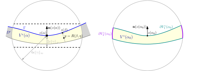
(a)                                                                       (b)

Figure 4. (a) In Step 1, $V^{\epsilon}(\alpha)$ (the yellow set) must lie between the two dashed lines for small $\epsilon$. (b) In Step 2, $\partial V^{\epsilon}(\alpha_{0})$ is decomposed into $\partial V_{1}^{\epsilon}(\alpha_{0})$ (in dark green) and $\partial V_{2}^{\epsilon}(\alpha_{0})$ (in purple).

Step 2. Next we prove (4.16). Note that $v^{\epsilon}$ is superharmonic in $D^{\epsilon}$ and vanishes on the boundary, thus it follows from the maximum principle that $v^{\epsilon}\geq 0$ in $D^{\epsilon}$. Denote $M:=\max_{x\in D^{\epsilon}}v(x)$, and pick $x_{0}=R(\alpha_{0},\eta_{0})\in D^{\epsilon}$ such that $v(x_{0})=M$. Without loss of generality, we can assume that $z(\alpha_{0})=(0,0)$ and $\mathbf{s}(z(\alpha_{0}))=\mathbf{e}_{1}:=(1,0)$, so that $\mathbf{n}(z(\alpha_{0}))=(0,1)$ and $x_{0}=(0,\epsilon\gamma(\alpha_{0})\eta_{0})$. Let us consider a barrier function $b_{1}:\mathbb{R}^{2}\mapsto\mathbb{R}$ given by

$$b_{1}(x_{1},x_{2})=x_{2}^{2}-\frac{x_{1}^{2}}{2}.$$

Clearly $\Delta b_{1}=1$, so $v^{\epsilon}+b_{1}$ is harmonic in $D^{\epsilon}$. It then follows from the maximum principle that $\max_{\overline{V^{\epsilon}(\alpha_{0})}}(v^{\epsilon}+b_{1})$ is achieved at some boundary point $\tilde{x}_{0}\in\partial V^{\epsilon}(\alpha_{0})$. Let us break $\partial V^{\epsilon}(\alpha_{0})$ into $\partial V^{\epsilon}_{1}(\alpha_{0})\cup\partial V^{\epsilon}_{2}(\alpha_{0})$ (see Figure 4(b) for an illustration), given by

$$\partial V^{\epsilon}_{1}(\alpha_{0}):=\partial D^{\epsilon}\cap B_{6\epsilon\rVert\gamma\rVert_{\infty}}(z(\alpha_{0})),\quad\partial V^{\epsilon}_{2}(\alpha_{0}):=\overline{D^{\epsilon}}\cap\partial B_{6\epsilon\rVert\gamma\rVert_{\infty}}(z(\alpha_{0})).$$ (4.24)

We claim that $\tilde{x}_{0}\in\partial V^{\epsilon}_{1}(\alpha_{0})$. To see this, note that any $y=(y_{1},y_{2})\in\partial V^{\epsilon}_{2}(\alpha_{0})$ satisfies $|y|=6\epsilon\rVert\gamma\rVert_{\infty}$ and $|y_{2}|\leq 2\epsilon\rVert\gamma\rVert_{\infty}$, where the latter follows from (4.18) and our assumption that $\mathbf{s}(z(\alpha_{0}))=\mathbf{e}_{1}$. This implies that $|y_{1}|\geq 4\epsilon\rVert\gamma\rVert_{\infty}>|y_{2}|$, thus $b_{1}(y)<0$. Using that $v^{\epsilon}(x_{0})=M\geq v^{\epsilon}(y)$ and $b_{1}(x_{0})=b_{1}(0,\epsilon\gamma(\alpha_{0})\eta_{0})\geq 0$, we have $(v^{\epsilon}+b_{1})(y)<(v^{\epsilon}+b_{1})(x_{0}).$ This shows that $\max_{\overline{V^{\epsilon}(\alpha_{0})}}(v^{\epsilon}+b_{1})$ cannot be achieved on $\partial V^{\epsilon}_{2}(\alpha_{0})$, finishing the proof of the claim.

Since $\tilde{x}_{0}\in\partial V^{\epsilon}_{1}(\alpha_{0})\subset\partial D^{\epsilon}$, the boundary condition in (4.15) yields that $v^{\epsilon}(\tilde{x}_{0})=0$. Thus

$$M+b_{1}(x_{0})=v^{\epsilon}(x_{0})+b_{1}(x_{0})\leq v^{\epsilon}(\tilde{x}_{0})+b_{1}(\tilde{x}_{0})=b_{1}(\tilde{x}_{0}).$$

Using $b_{1}(x_{0})=b_{1}(0,\epsilon\gamma(\alpha_{0})\eta_{0})\geq 0$, the above inequality becomes

$$M\leq b_{1}(\tilde{x}_{0})\leq|\tilde{x}_{0}|^{2}\leq 36\rVert\gamma\rVert_{\infty}^{2}\epsilon^{2},$$ (4.25)

where the second inequality follows from the definition of $b_{1}$. This proves (4.16) for $C_{1}=36\rVert\gamma\rVert_{\infty}^{2}$.

Step 3. It remains to prove (4.17). First note that for $i\in\{1,\dots,n\}$, the assumptions (H1)–(H3) yield that $D_{i}^{\epsilon}$ has $C^{2}$ boundary, therefore $v^{\epsilon}\in C^{2}(D_{i}^{\epsilon})\cap C^{1}(\overline{D_{i}^{\epsilon}})$. Let us fix $i\in\left\{1,\ldots,n\right\}$ and any $\alpha\in S$, and we aim to show that $|\nabla v^{\epsilon}(z(\alpha))|\leq C_{2}\epsilon$. Again, without loss of generality we can assume that $z(\alpha)=(0,0)$ and $\mathbf{s}(z(\alpha))=\mathbf{e}_{1}$. Let us consider a new barrier function $b_{2}:\mathbb{R}^{2}\to\mathbb{R}$

$$b_{2}(x_{1},x_{2}):=x_{2}^{2}+4\epsilon\rVert\gamma\rVert_{\infty}x_{2}-\frac{x_{1}^{2}}{2},$$ (4.26)

which satisfies $b_{2}(0,0)=0$, and one can easily check that its zero level set has horizontal tangent at $(0,0)$ (thus tangent to $\partial D^{\epsilon}$ at $z(\alpha)$).

Again, let us decompose $\partial V^{\epsilon}(\alpha)$ as $\partial V^{\epsilon}_{1}(\alpha)\cup\partial V^{\epsilon}_{2}(\alpha)$ as in (4.24) (except that $\alpha_{0}$ now becomes $\alpha$). We claim that for all sufficiently small $\epsilon>0$, the new barrier function $b_{2}$ satisfies

$$\Delta b_{2}=1~{}~{}~{}\,\text{ in }V^{\epsilon}(\alpha),$$ (4.27)

$$b_{2}\leq 0\quad~{}~{}~{}\text{ on }\partial V^{\epsilon}_{1},$$ (4.28)

$$b_{2}\leq-\epsilon^{2}\quad\text{ on }\partial V^{\epsilon}_{2}.$$ (4.29)

Let us assume for a moment that (4.27)–(4.29) are true. Then it follows that

$$v^{\epsilon}+C_{2}b_{2}\leq 0\text{ in }V^{\epsilon}(\alpha),$$ (4.30)

where $C_{2}:=\max\left\{1,C_{1}\right\}$ and $C_{1}$ is as in (4.16) (in the end of step 2 we have $C_{1}=36\rVert\gamma\rVert_{\infty}^{2}$). To show (4.30), note that $v^{\epsilon}+C_{2}b_{2}$ is subharmonic in $V^{\epsilon}(\alpha)$ due to (4.27) and the definition of $C_{2}$, thus its maximum is attained on its boundary. The boundary conditions in (4.15) and (4.28) yield that $v^{\epsilon}+C_{2}b_{2}\leq 0$ on $\partial V^{\epsilon}_{1}(\alpha)$; whereas (4.16), (4.29) and the definition of $C_{2}$ yield that $v^{\epsilon}+C_{2}b_{2}\leq 0$ on $\partial V^{\epsilon}_{2}(\alpha)$. Thus $v^{\epsilon}+C_{2}b_{2}\leq 0$ on $\partial V^{\epsilon}_{1}(\alpha)\cup\partial V^{\epsilon}_{2}(\alpha)$, implying (4.30).

However, $v^{\epsilon}+C_{2}b_{2}$ is actually zero at $z(\alpha)\in\partial V^{\epsilon}(\alpha)$, therefore Hopf’s Lemma implies that $\nabla\left(v^{\epsilon}+C_{2}b_{2}\right)(z(\alpha))\cdot\vec{n}(z(\alpha))>0$, where $\vec{n}(z(\alpha))$ is the outer normal of $\partial D^{\epsilon}$ at $z(\alpha)$. Hence

$$|\nabla v^{\epsilon}(z(\alpha))|=-\nabla v^{\epsilon}(z(\alpha))\cdot\vec{n}(z(\alpha))<C_{2}\nabla b_{2}(z(\alpha))\cdot\vec{n}(z(\alpha))=4C_{2}\rVert\gamma\rVert_{\infty}\epsilon,$$ (4.31)

where the first equality follows from the fact that $v^{\epsilon}$ is superharmonic in $D^{\epsilon}$ and constant on $\partial D^{\epsilon}$, and the second equality is a direct computation of $\nabla b_{2}$. Thus (4.31) proves (4.17).

To complete the proof, we only need to prove (4.27)–(4.29) for small $\epsilon>0$. Note that (4.27) follows immediately from computing the Laplacian of $b_{2}$. For (4.28), let us pick $y\in\partial V^{\epsilon}_{1}(\alpha)$, and we aim to show that $b_{2}(y)\leq 0$. Note that $y=R^{\epsilon}(\beta,0)$ or $R^{\epsilon}(\beta,-1)$ for some $\beta\in S$. We first deal with the first case.

Let us denote $y=(y_{1},y_{2})$. Rewriting (4.20) into two inequalities for the two components, and using that $z(\alpha)=(0,0)$ and $z^{\prime}(\alpha)=L\mathbf{e}_{1}$ ($L$ is the length of the curve $\Gamma_{i}$), we have

$$|0-y_{1}-L(\alpha-\beta)|\leq\|z^{\prime\prime}\|_{\infty}(\alpha-\beta)^{2}$$ (4.32)

$$|y_{2}|=|0-y_{2}|\leq\|z^{\prime\prime}\|_{\infty}(\alpha-\beta)^{2}.$$ (4.33)

Also, (4.22) gives $|\alpha-\beta|\leq 7F_{\Gamma}\|\gamma\|_{\infty}\epsilon$. Applying it to (4.32), for all $\epsilon>0$ sufficiently small we have that

$$|y_{1}|\geq\frac{L}{2}|\alpha-\beta|.$$ (4.34)

Plugging (4.34) and (4.33) into $b_{2}(y)=-\frac{1}{2}y_{1}^{2}+y_{2}^{2}+4\epsilon\|\gamma\|_{\infty}y_{2}$, we have

$$\begin{split}b_{2}(y)&\leq-\frac{L^{2}}{8}(\alpha-\beta)^{2}+\|z^{\prime\prime}\|_{\infty}^{2}(\alpha-\beta)^{4}+4\epsilon\|\gamma\|_{\infty}\|z^{\prime\prime}\|_{\infty}(\alpha-\beta)^{2}\\ &\leq\left(-\frac{L^{2}}{8}+C\epsilon^{2}+C\epsilon\right)(\alpha-\beta)^{2}\leq 0,\end{split}$$

for all $\epsilon>0$ sufficiently small, where the second inequality follows from (4.22). This finishes the proof of (4.28) for the case $y=R^{\epsilon}(\beta,0)$.

Before we deal with the case $y=R^{\epsilon}(\beta,-1)$, let us prove (4.29) first. For any $y=(y_{1},y_{2})\in\partial V^{\epsilon}_{2}(\alpha)$, (4.18) gives $|y_{2}|\leq 2\epsilon\|\gamma\|_{\infty}$. Combining this with $|y|=6\epsilon\|\gamma\|_{\infty}$ yields $|y_{1}|\geq\sqrt{32}\epsilon\rVert\gamma\rVert_{\infty}$. Thus

$$b_{2}(y)\leq(2\epsilon\|\gamma\|_{\infty})^{2}+4\epsilon\rVert\gamma\rVert_{\infty}(2\epsilon\|\gamma\|_{\infty})-\frac{(\sqrt{32}\epsilon\rVert\gamma\rVert_{\infty})^{2}}{2}\leq-4\epsilon^{2}\|\gamma\|_{\infty}^{2}.$$

Finally we turn to the proof of (4.28) for the case $y=R^{\epsilon}(\beta,-1)$. Note that the curve $\{R^{\epsilon}(\beta,-1):\beta\in S\}\cap B_{6\epsilon\|\gamma\|_{\infty}}(z(\alpha))$ lies in the interior of the region bounded by $\Gamma\cap B_{6\epsilon\|\gamma\|_{\infty}}(z(\alpha))$ on the top, $\partial B_{6\epsilon\|\gamma\|_{\infty}}(z(\alpha))$ on the sides, and $y_{2}=-2\epsilon\|\gamma\|_{\infty}$ on the bottom. (The last one follows from (4.18) and our assumption that $\mathbf{s}(z(\alpha))=\mathbf{e}_{1}$). We have already shown $b_{2}\leq 0$ on $\Gamma\cap B_{6\epsilon\|\gamma\|_{\infty}}(z(\alpha))$ and the lateral boundaries, and it is easy to check that $b_{2}\leq 0$ on $y_{2}=-2\epsilon\|\gamma\|_{\infty}$. Since the set $\{b_{2}\leq 0\}$ is simply-connected, it implies that $b_{2}\leq 0$ in the interior of this region, finishing the proof. ∎

Note that (4.16) of Lemma 4.4 immediately implies Proposition 4.2. (The only difference is that $\Delta v^{\epsilon}=-1$ in Lemma 4.4 whereas $\Delta p^{\epsilon}=-2$ in Proposition 4.2, so the constant $C$ in Proposition 4.2 is twice of that in (4.16)). The lemma also implies the following corollary, which will be helpful in the proof of Proposition 4.3.

Corollary 4.5.

For any $i=1,\dots,n+m$, assume $\Gamma_{i}$ and $\gamma_{i}$ satisfy (H1)–(H3). Assume $v^{\epsilon}\in C^{2}(D^{\epsilon}_{i})\cap C(\overline{D^{\epsilon}_{i}})$ satisfies that

$$\begin{cases}\left|\Delta v^{\epsilon}\right|\leq C_{0}&\text{ in }D^{\epsilon}_{i},\\ v^{\epsilon}=0&\text{ on }\partial D^{\epsilon}_{i},\end{cases}$$

for some constant $C_{0}>0$. Then for the same constants $\epsilon_{0},C_{1},C_{2}$ as in Lemma 4.4, the following holds for all $\epsilon\in(0,\epsilon_{0})$:

$$|v^{\epsilon}|\leq C_{0}C_{1}\epsilon^{2}\quad\text{ in }D^{\epsilon}_{i},$$ (4.35)

and if $v^{\epsilon}\in C^{2}(D^{\epsilon}_{i})\cap C^{1}(\overline{D^{\epsilon}_{i}})$, we have

$$\rVert\nabla v^{\epsilon}\rVert_{L^{\infty}(\Gamma_{i})}\leq C_{0}C_{2}\epsilon\quad\text{ for }\quad i=1,\ldots,n.$$ (4.36)

Proof.

Let $\tilde{v}$ be a solution to

$$\begin{cases}\Delta\tilde{v}=-C_{0}&\text{ in }D^{\epsilon}_{i},\\ \tilde{v}=0&\text{ on }\partial D^{\epsilon}_{i}.\end{cases}$$

It is clear that $v^{\epsilon}+\tilde{v}$ is super-harmonic and $v^{\epsilon}-\tilde{v}$ is sub-harmonic in $D^{\epsilon}_{i}$, and they both vanish on the boundary. Thus the maximum principle implies that

$$-\tilde{v}\leq v^{\epsilon}\leq\tilde{v}\quad\text{ in }D^{\epsilon}_{i}.$$ (4.37)

Applying (4.16) of Lemma 4.4 to $\frac{\tilde{v}}{C_{0}}$, we obtain $0\leq\tilde{v}\leq C_{0}C_{1}\epsilon^{2}$ in $D^{\epsilon}_{i}$ for all $\epsilon\in(0,\epsilon_{0})$, leading to (4.35). Furthermore, (4.37) and the fact that $v^{\epsilon}$ and $v$ both have zero boundary condition imply that

$$|\nabla v^{\epsilon}|\leq|\nabla\tilde{v}|\quad\text{ on }\partial D^{\epsilon}_{i}.$$

We then apply (4.17) of Lemma 4.4 to $\frac{\tilde{v}}{C_{0}}$ and obtain $\rVert\nabla v^{\epsilon}\rVert_{L^{\infty}(\Gamma_{i})}\leq C_{0}C_{2}\epsilon,$ which proves (4.36). ∎

Now we are ready to prove Proposition 4.3.

Proof of Proposition 4.3.

Throughout the proof, let $i\in\{1,\dots,n\}$ be fixed. For notational simplicity, in the rest of the proof we omit the subscript $i$ from all terms.

We claim that

$$\left|\nabla\tilde{p}^{\epsilon}(R^{\epsilon}(\alpha,\eta))-\frac{c^{\epsilon}}{\epsilon\gamma(\alpha)}\mathbf{n}(z(\alpha))\right|\leq C\epsilon\quad\text{ for all }\alpha\in S,\eta\in[0,-1],$$ (4.38)

$$\rVert\Delta q^{\epsilon}\rVert_{L^{\infty}(D^{\epsilon})}\leq C$$ (4.39)

for some constant $C>0$ only depending on $\rVert z_{i}\rVert_{C^{3}(S_{i})},\rVert\gamma_{i}\rVert_{C^{2}(S_{i})}$ and $F_{\Gamma}$. Assuming these are true, let us explain how they lead to (4.12)–(4.14). By (4.6) and (4.10), $p^{\epsilon}$ and $\tilde{p}^{\epsilon}$ have the same boundary condition, thus $q^{\epsilon}=0$ on $\partial D^{\epsilon}$. This and (4.39) allow us to apply Corollary 4.5 to $q^{\epsilon}$ to obtain the estimate (4.35), implying (4.12).

Due to (4.36) of Corollary 4.5, we also have

$$\rVert\nabla q^{\epsilon}\rVert_{L^{\infty}(\Gamma)}\leq C\epsilon.$$ (4.40)

Using (4.7) and $p^{\epsilon}=\tilde{p}^{\epsilon}+q^{\epsilon}$, we have

$$-2|U| =\int_{\partial U}\nabla\tilde{p}^{\epsilon}\cdot{n}d\sigma+\int_{\partial U}\nabla q^{\epsilon}\cdot nd\sigma$$

$$=-\frac{c^{\epsilon}L}{\epsilon}\int_{S}\gamma^{-1}(\alpha)d\alpha+O(\epsilon),$$

where the second equality follows from (4.38) for $\eta=0$, $n(z(\alpha))=-\mathbf{n}(z(\alpha))$ and $d\sigma=Ld\alpha$, as well as (4.40). Rearranging the terms and using the definition of $\beta$ in (4.11) yields (4.13).

Finally, note that (4.13) and (4.38) directly lead to (4.14), where we are using the fact that $\gamma_{i}$ is uniformly positive for $i=1,\dots,n$, due to (H3).

The rest of the proof is devoted to proving the claims (4.38) and (4.39). For (4.38), we compute the gradient of $\tilde{p}^{\epsilon}$. Differentiating (4.10) with respect to $\alpha$ and $\eta$, we obtain

$$(\nabla_{\alpha,\eta}R^{\epsilon}(\alpha,\eta))^{t}\nabla\tilde{p}(R^{\epsilon}(\alpha,\eta))=\begin{pmatrix}0\\ c^{\epsilon}\end{pmatrix},$$ (4.41)

where $(\nabla_{\alpha,\eta}R^{\epsilon})^{t}$ denotes the transpose of the Jacobian matrix of $R^{\epsilon}$. Since $\nabla_{\alpha,\eta}R^{\epsilon}=(\partial_{\alpha}R^{\epsilon},\partial_{\eta}R^{\epsilon})$, using the formula for inverses of $2\times 2$ matrices, we have

$$\left(\left(\nabla_{\alpha,\eta}R^{\epsilon}\right)^{t}\right)^{-1}=\frac{1}{J(\alpha,\eta)}\big{(}\!-\!(\partial_{\eta}R^{\epsilon})^{\perp},(\partial_{\alpha}R^{\epsilon})^{\perp}\big{)}.$$ (4.42)

where $J(\alpha,\eta):=\text{det}(\nabla_{\alpha,\eta}R^{\epsilon})$. Multiplying the inverse matrix on both sides of (4.41), we have

$$\nabla\tilde{p}^{\epsilon}(R^{\epsilon}(\alpha,\eta))=\frac{1}{J}\big{(}\!-\!(\partial_{\eta}R^{\epsilon})^{\perp},(\partial_{\alpha}R^{\epsilon})^{\perp}\big{)}\begin{pmatrix}0\\ c^{\epsilon}\end{pmatrix}=\frac{c^{\epsilon}}{J}(\partial_{\alpha}R^{\epsilon})^{\perp}.$$ (4.43)

Recall that Lemma 3.2 gives $(\partial_{\alpha}R^{\epsilon})^{\perp}=z^{\prime}(\alpha)^{\perp}+O(\epsilon)=L\mathbf{n}(z(\alpha))+O(\epsilon)$, and $J=\epsilon L\gamma+O(\epsilon^{2})$. Plugging these into (4.43) gives

$$\nabla\tilde{p}^{\epsilon}(R(\alpha,\eta))=\frac{c^{\epsilon}}{\epsilon}\left(\frac{\mathbf{n}(z(\alpha))}{\gamma}+O(\epsilon)\right).$$ (4.44)

Note that it follows from (4.8) that $c^{\epsilon}\leq\frac{|D^{\epsilon}|}{2\pi}$, where $|D^{\epsilon}|\leq C\epsilon$ due to (3.9). These imply

$$\frac{c_{\epsilon}}{\epsilon}\leq C,$$ (4.45)

and applying it to (4.44) yields (4.38).

To prove (4.39), since $q^{\epsilon}=p^{\epsilon}-\tilde{p}^{\epsilon}$ and $\Delta p^{\epsilon}=-2$ in $D^{\epsilon}$, it suffices to show that

$$\left|\Delta\tilde{p}^{\epsilon}\right|\leq C\quad\text{ in }D^{\epsilon},$$ (4.46)

and we will begin with an explicit computation of $\partial_{x_{1}x_{1}}\tilde{p}^{\epsilon}$ and $\partial_{x_{2}x_{2}}\tilde{p}^{\epsilon}$. Let us denote $R^{\epsilon}=:(R^{1},R^{2})$. For notational simplicity, in the rest of the proof we will use subscripts on $R^{\epsilon}$, $R^{1}$, $R^{2}$ and $J$ to denote their partial derivative, e.g. $R^{1}_{\alpha}:=\partial_{\alpha}R^{1}$.

From (4.43), it follows that

$$\partial_{x_{1}}\tilde{p}^{\epsilon}(R^{\epsilon}(\alpha,\eta))=-\frac{c^{\epsilon}}{J}R^{2}_{\alpha}.$$

Differentiating in $\alpha$ and $\eta$, we get

$$\begin{split}\nabla\left(\partial_{x_{1}}\tilde{p}^{\epsilon}\right)(R^{\epsilon}(\alpha,\eta))&=\left(\left(\nabla_{\alpha,\eta}R^{\epsilon}\right)^{t}\right)^{-1}\nabla_{\alpha,\eta}\left(-\frac{c^{\epsilon}}{J}R^{2}_{\alpha}\right)\\ &=\frac{c^{\epsilon}}{J}\begin{pmatrix}R_{\eta}^{2}&-R_{\alpha}^{2}\\[2.84544pt] -R_{\eta}^{1}&R_{\alpha}^{1}\end{pmatrix}\begin{pmatrix}\frac{J_{\alpha}}{J^{2}}R^{2}_{\alpha}-\frac{1}{J}R^{2}_{\alpha\alpha}\\[2.84544pt] \frac{J_{\eta}}{J^{2}}R_{\alpha}^{2}-\frac{1}{J}R^{2}_{\alpha\eta}\end{pmatrix},\end{split}$$

thus

$$\partial_{x_{1}x_{1}}\tilde{p}^{\epsilon}(R(\alpha,\eta))=\frac{c^{\epsilon}}{J}\left(\frac{J_{\alpha}}{J^{2}}R^{2}_{\eta}R^{2}_{\alpha}-\frac{1}{J}R^{2}_{\eta}R^{2}_{\alpha\alpha}-\frac{J_{\eta}}{J^{2}}(R_{\alpha}^{2})^{2}+\frac{1}{J}R^{2}_{\alpha}R^{2}_{\alpha\eta}\right).$$

Likewise, $\partial_{x_{2}x_{2}}\tilde{p}(R(\alpha,\eta))$ takes the same expression except every $R^{2}$ is changed into $R^{1}$. Adding them together gives

$$\Delta\tilde{p}^{\epsilon}(R(\alpha,\eta))=\frac{c^{\epsilon}}{J}\left(\frac{J_{\alpha}}{J^{2}}R^{\epsilon}_{\eta}\cdot R^{\epsilon}_{\alpha}-\frac{1}{J}R_{\eta}^{\epsilon}\cdot R^{\epsilon}_{\alpha\alpha}-\frac{J_{\eta}}{J^{2}}R^{\epsilon}_{\alpha}\cdot R^{\epsilon}_{\alpha}+\frac{1}{J}R^{\epsilon}_{\alpha}\cdot R^{\epsilon}_{\alpha\eta}\right).$$ (4.47)

Using the explicit formulae of $R_{\alpha},R_{\eta}$ and $J$ in Lemma 3.2, we directly obtain $|R^{\epsilon}_{\alpha}|,|R^{\epsilon}_{\alpha\alpha}|\leq C$;  $|R^{\epsilon}_{\eta}|,|R^{\epsilon}_{\alpha\eta}|,|J_{\alpha}|\leq C\epsilon$;  $|J_{\eta}|\leq C\epsilon^{2}$;  and $J^{-1}\leq C\epsilon^{-1}$ when $\epsilon$ is sufficiently small, where $C$ depends on $\rVert z_{i}\rVert_{C^{3}(S_{i})}$ and $\rVert\gamma_{i}\rVert_{C^{2}(S_{i})}$. As a result, all the four terms in the parenthesis of (4.47) are bounded by some constant $C$ independent of $\epsilon$. Finally, (4.45) yields $\frac{c_{\epsilon}}{J}\leq C$ as well, thus $|\Delta\tilde{p}^{\epsilon}|\leq C$, and this proves the second claim (4.39). ∎

5. Proof of the symmetry result

In this section we prove that a stationary vortex sheet with positive vorticity must be radially symmetric up to a translation, and a rotating vortex sheet with positive vorticity and angular velocity $\Omega<0$ must be radially symmetric. The key idea of the proof is to define the integral

$$\begin{split}I^{\epsilon}&:=\int_{D^{\epsilon}}\epsilon^{-1}\mathbf{u}^{\epsilon}\cdot\nabla\left(\omega^{\epsilon}*\mathcal{N}-\frac{\Omega}{2}|x|^{2}\right)dx\\ &=\int_{D^{\epsilon}}\epsilon^{-1}(x+\nabla p^{\epsilon})\cdot\nabla\left(\omega^{\epsilon}*\mathcal{N}-\frac{\Omega}{2}|x|^{2}\right)dx,\end{split}$$ (5.1)

and compute it in two different ways. The motivation of the definition is as follows. As discussed in [14, Section 2.1], $I^{\epsilon}$ can be thought of as a first variation of an “energy functional”

$$\mathcal{E}[\omega^{\epsilon}]:=\int\frac{1}{2}\omega^{\epsilon}(\omega^{\epsilon}*\mathcal{N})-\frac{\Omega}{2}\omega^{\epsilon}|x|^{2}\,dx$$

when we perturb $\omega^{\epsilon}$ by a divergence free vector $\mathbf{u}^{\epsilon}$ in $D^{\epsilon}$. (This functional $\mathcal{E}$ only serves as our motivation, and will not appear in the proof.) On the one hand, using that $\omega_{0}$ is stationary in the rotating frame with angular velocity $\Omega$ and $\omega^{\epsilon}$ is a close approximation of $\omega_{0}$, we will show in Proposition 5.1 that $I^{\epsilon}$ is of order $O(\epsilon|\log\epsilon|)$, thus goes to zero as $\epsilon\to 0$. On the other hand, using the particular $\mathbf{u}^{\epsilon}$ that we constructed in Section 4, we will prove in Proposition 5.2 that if $\Omega=0$, $I^{\epsilon}$ is strictly positive independently of $\epsilon$ unless all the vortex sheets are nested circles with constant density; and also prove a similar result in Corollary 5.3 for $\Omega<0$.

Proposition 5.1.

Assume $\omega(\cdot,t)=\omega_{0}(R_{\Omega t}\cdot)$ is a stationary/uniformly-rotating vortex sheet with angular velocity $\Omega\in\mathbb{R}$, where $\omega_{0}$ satisfies (H1)–(H3). Then there exists some $C>0$ only depending on $b$ (as in (H2)), $\max_{i}\|z_{i}\|_{C^{3}(S_{i})}$, $\max_{i\leq n}\|\gamma_{i}\|_{C^{2}(S_{i})}$, $\max_{i>n}\|\gamma_{i}\|_{C^{b}(S_{i})}$, $d_{\Gamma}$ and $F_{\Gamma}$, such that $|I^{\epsilon}|<C\epsilon^{b}|\log\epsilon|$ for all sufficiently small $\epsilon>0$.

Proof.

Let us decompose $I^{\epsilon}=:\sum_{i=1}^{n+m}I^{\epsilon}_{i}$, where $I_{i}^{\epsilon}:=\int_{D^{\epsilon}_{i}}\epsilon^{-1}(x+\nabla p^{\epsilon})\cdot\nabla(\omega^{\epsilon}*\mathcal{N}-\frac{\Omega}{2}|x|^{2})dx.$

We start with showing that $|I^{\epsilon}_{i}|\leq C\epsilon^{b}|\log\epsilon|$ for $i=n+1,\dots,n+m$. For such $i$, $p^{\epsilon}=0$ on $\partial D^{\epsilon}_{i}$, thus the divergence theorem (and the fact that $\omega^{\epsilon}=\epsilon^{-1}$ in $D^{\epsilon}_{i}$) gives

$$I^{\epsilon}_{i}=\underbrace{\int_{D^{\epsilon}_{i}}\epsilon^{-1}x\cdot\nabla\left(\omega^{\epsilon}*\mathcal{N}-\frac{\Omega}{2}|x|^{2}\right)dx}_{=:T_{i}^{\epsilon}}-\int_{D^{\epsilon}_{i}}\epsilon^{-1}(\epsilon^{-1}-2\Omega)p^{\epsilon}(x)dx.$$

Using the estimate $|p^{\epsilon}|\leq C\epsilon^{2}$ in Proposition 4.2 and the fact that $|D^{\epsilon}_{i}|\leq C\epsilon$ from (3.9), we easily bound the second integral by $C\epsilon$. To control the first integral $T_{i}^{\epsilon}$, we rewrite it using the change of variables $x=R^{\epsilon}_{i}(\alpha,\eta)$ and the definition $\mathbf{v}^{\epsilon}:=\nabla^{\perp}(\omega^{\epsilon}*\mathcal{N})$ in (3.10): (also note that on the right hand side we group $\epsilon^{-1}$ with the determinant)

$$\begin{split}T_{i}^{\epsilon}=\int_{S_{i}}\int_{-1}^{0}R_{i}^{\epsilon}(\alpha,\eta)\cdot\underbrace{\Big{(}\!-\!(\mathbf{v}^{\epsilon})^{\perp}(R_{i}^{\epsilon}(\alpha,\eta))-\Omega R_{i}^{\epsilon}(\alpha,\eta)\Big{)}}_{=:J_{i}^{\epsilon}}\underbrace{\epsilon^{-1}\det(\nabla_{\alpha,\eta}R_{i}^{\epsilon}(\alpha,\eta))}_{=:K_{i}^{\epsilon}}\,d\eta d\alpha.\end{split}$$

Let us take a closer look at the integrand, which is a product of 3 terms. Clearly, the definition of $R_{i}^{\epsilon}$ gives $R_{i}^{\epsilon}(\alpha,\eta)=z_{i}(\alpha)+O(\epsilon).$ As for the middle term $J_{i}^{\epsilon}$, Lemma 3.4 yields

$$J_{i}^{\epsilon}(\alpha,\eta)=-BR^{\perp}(z_{i}(\alpha))+\left(\eta+\frac{1}{2}\right)[\mathbf{v}]^{\perp}(z_{i}(\alpha))-\Omega z_{i}(\alpha)+O(\epsilon^{b}|\log\epsilon|).$$ (5.2)

Using the fact that $BR(z_{i}(\alpha))=\Omega z_{i}^{\perp}(\alpha)$ for $i=n+1,\dots,n+m$ (which follows from (2.6) and (2.7)), it becomes

$$J_{i}^{\epsilon}(\alpha,\eta)=\left(\eta+\frac{1}{2}\right)[\mathbf{v}]^{\perp}(z_{i}(\alpha))+O(\epsilon^{b}|\log\epsilon|).$$ (5.3)

Also it follows from (3.8) that $K_{i}^{\epsilon}(\alpha,\eta)=L_{i}\gamma_{i}(\alpha)+O(\epsilon).$ Plugging these three estimates into the above integral gives

$$T_{i}^{\epsilon}=\int_{S_{i}}\int_{-1}^{0}z_{i}(\alpha)\cdot\left(\eta+\frac{1}{2}\right)[\mathbf{v}]^{\perp}(z_{i}(\alpha))L_{i}\gamma_{i}(\alpha)d\eta d\alpha+O(\epsilon^{b}|\log\epsilon|)=O(\epsilon^{b}|\log\epsilon|),$$

where the last step follows from the fact that $\int_{-1}^{0}(\eta+\frac{1}{2})d\eta=0$. This finishes the proof that $|I^{\epsilon}_{i}|\leq C\epsilon^{b}|\log\epsilon|$ for $i=n+1,\dots,n+m$, where $C$ depends on $b$, $\max_{i}\|z_{i}\|_{C^{2}(S_{i})}$, $\max_{i}\|\gamma_{i}\|_{C^{b}(S_{i})}$, $d_{\Gamma}$ and $F_{\Gamma}$.

In the rest of the proof we aim to show $|I^{\epsilon}_{i}|\leq C\epsilon^{b}|\log\epsilon|$ for $i=1,\dots,n$, which is slightly more involved. Recall that in Proposition 4.3 we defined $\tilde{p}^{\epsilon}$ and $q^{\epsilon}$ in $D_{i}^{\epsilon}$ for $i=1,\dots,n$, where they satisfy $p^{\epsilon}=\tilde{p}^{\epsilon}+q^{\epsilon}$ in $D_{i}^{\epsilon}$, and $q^{\epsilon}=0$ on $\partial D_{i}^{\epsilon}$. This allows us to apply the divergence theorem (to the $q^{\epsilon}$ term only) and decompose $I_{i}^{\epsilon}$ as

$$I^{\epsilon}_{i}=\int_{D^{\epsilon}_{i}}\epsilon^{-1}(x+\nabla\tilde{p}_{\epsilon})\cdot\nabla\left(\omega^{\epsilon}*\mathcal{N}-\frac{\Omega}{2}|x|^{2}\right)dx-\int_{D^{\epsilon}_{i}}\epsilon^{-1}(\epsilon^{-1}-2\Omega)q^{\epsilon}(x)dx=:I^{\epsilon}_{i,1}+I^{\epsilon}_{i,2}.$$

We can easily show that $I^{\epsilon}_{i,2}=O(\epsilon)$: (4.12) of Proposition 4.3 gives $|q^{\epsilon}|\leq C\epsilon^{2}$, and combining it with $|D^{\epsilon}_{i}|\leq C\epsilon$ in (3.9) immediately yields the desired estimate.

Next we turn to $I^{\epsilon}_{i,1}$. Again, the change of variables $x=R^{\epsilon}_{i}(\alpha,\eta)$ and the definition $\mathbf{v}^{\epsilon}:=\nabla^{\perp}(\omega^{\epsilon}*\mathcal{N})$ gives

$$I_{i,1}^{\epsilon}=\int_{S_{i}}\int_{-1}^{0}\big{(}R_{i}^{\epsilon}(\alpha,\eta)+\nabla\tilde{p}^{\epsilon}(R_{i}^{\epsilon}(\alpha,\eta))\big{)}\cdot\underbrace{\Big{(}\!-\!(\mathbf{v}^{\epsilon})^{\perp}(R_{i}^{\epsilon}(\alpha,\eta))-\Omega R_{i}^{\epsilon}(\alpha,\eta)\Big{)}}_{=:J_{i}^{\epsilon}}\underbrace{\epsilon^{-1}\det(\nabla_{\alpha,\eta}R_{i}^{\epsilon}(\alpha,\eta))}_{=:K_{i}^{\epsilon}}\,d\eta d\alpha.$$

For the three terms in the product of the integrand, we will approximate the first term using the definition of $R_{i}^{\epsilon}$ and (4.14) of Proposition 4.3:

$$R_{i}^{\epsilon}(\alpha,\eta)+\nabla\tilde{p}^{\epsilon}(R_{i}^{\epsilon}(\alpha,\eta))=z_{i}(\alpha)+\frac{\beta_{i}}{\gamma_{i}(\alpha)}\mathbf{n}(z_{i}(\alpha))+O(\epsilon),$$

where $\beta_{i}:=\frac{2|U_{i}|}{L_{i}\int_{S_{i}}\gamma_{i}^{-1}(\alpha)d\alpha}$ is given by (4.11). Lemma 3.4 allows us to approximate the middle term $J_{i}^{\epsilon}$ as (5.2), however (5.3) no longer holds since for $i=1,\dots,n$ we do not have $BR(z_{i}(\alpha))=\Omega z_{i}^{\perp}(\alpha)$. As for $K_{i}^{\epsilon}$, we again use (3.8) to approximate it by $K_{i}^{\epsilon}(\alpha,\eta)=L_{i}\gamma_{i}(\alpha)+O(\epsilon).$ Plugging these three estimates into the integrand of $I_{i,1}^{\epsilon}$ gives

$$I_{i,1}^{\epsilon}=\int_{S_{i}}\left(z_{i}(\alpha)+\frac{\beta_{i}}{\gamma_{i}(\alpha)}\mathbf{n}(z_{i}(\alpha))\right)\cdot\Big{(}-\!\!BR^{\perp}(z_{i}(\alpha))-\Omega z_{i}(\alpha)\Big{)}L_{i}\gamma_{i}(\alpha)d\alpha+O(\epsilon^{b}|\log\epsilon|),$$

where we again use the fact that the $(\eta+\frac{1}{2})$ term gives zero contribution since $\int_{-1}^{0}(\eta+\frac{1}{2})d\eta=0$. Next we will show the integral on the right hand side is in fact 0. Since $\omega$ is a rotating solution with angular velocity $\Omega$, the conditions (2.6) and (2.7) yield that

$$-BR^{\perp}(z_{i}(\alpha))-\Omega z_{i}(\alpha)=C_{i}\gamma_{i}^{-1}(\alpha)\mathbf{n}(z_{i}(\alpha)),$$

for some constant $C_{i}$. Plugging this into the above integral gives

$$\begin{split}I_{i,1}^{\epsilon}&=C_{i}L_{i}\int_{S_{i}}\left(z_{i}(\alpha)\cdot\mathbf{n}(z_{i}(\alpha))+\frac{\beta_{i}}{\gamma_{i}(\alpha)}\right)d\alpha+O(\epsilon^{b}|\log\epsilon|)\\ &=C_{i}L_{i}\left(\int_{S_{i}}z_{i}(\alpha)\cdot\mathbf{n}(z_{i}(\alpha))d\alpha+\frac{2|U_{i}|}{L_{i}}\right)+O(\epsilon^{b}|\log\epsilon|),\end{split}$$

where the second step follows from the definition of $\beta_{i}$ in (4.11). Let us compute the integral on the right hand side by changing to arclength parametrization and applying the divergence theorem:

$$\int_{S_{i}}z_{i}(\alpha)\cdot\mathbf{n}(z_{i}(\alpha))d\alpha=-\frac{1}{L_{i}}\int_{\partial U_{i}}x\cdot nd\sigma=-\frac{2|U_{i}|}{L_{i}},$$

which yields $I_{i,1}^{\epsilon}=O(\epsilon^{b}|\log\epsilon|)$, and finishes the proof that $|I_{i}^{\epsilon}|\leq C\epsilon^{b}|\log\epsilon|$ for $i=1,\dots,n$, where $C$ depends on $b$, $\rVert z_{i}\rVert_{C^{3}(S_{i})},\rVert\gamma_{i}\rVert_{C^{2}(S_{i})}$, $d_{\Gamma}$ and $F_{\Gamma}$.

Finally, summing the $I_{i}^{\epsilon}$ estimates for $i=1,\dots,n+m$ gives $|I^{\epsilon}|\leq C\epsilon^{b}|\log\epsilon|$ for all sufficiently small $\epsilon>0$, thus we can conclude. ∎

Now we will use a different way to compute $I^{\epsilon}$. Let us first define a new integral $\tilde{I}^{\epsilon}$ that is the same as $I^{\epsilon}$ except with $\Omega$ set to zero:

$$\begin{split}\tilde{I}^{\epsilon}&:=\int_{D^{\epsilon}}\epsilon^{-1}(x+\nabla p^{\epsilon})\cdot\nabla\left(\omega^{\epsilon}*\mathcal{N}\right)dx.\end{split}$$ (5.4)

Next we will prove that $\tilde{I}^{\epsilon}$ is strictly positive independently of $\epsilon$ unless all the vortex sheets are nested circles with constant density. As we will see in the proof, the key step is to show that if some $\Gamma_{i}$ is either not a circle or does not have a constant $\gamma_{i}$, then the estimates on $p^{\epsilon}$ in Propositions 4.2–4.3 lead to the following quantitative version of (4.9): $\epsilon^{-2}\left(\frac{|D_{i}^{\epsilon}|^{2}}{4\pi}-\int_{D_{i}^{\epsilon}}p^{\epsilon}(x)dx\right)\geq c_{0}>0$, where $c_{0}$ is independent of $\epsilon$.

Proposition 5.2.

Let $\tilde{I}^{\epsilon}$ be defined as in (5.4). Assume that $\Gamma_{i}$ and $\gamma_{i}$ satisfy (H1)–(H3) for $i=1,\dots,n+m$. Then we have $\tilde{I}^{\epsilon}\geq 0$ for all sufficiently small $\epsilon>0$.

In addition, if $\Gamma$ is not a union of nested circles with constant $\gamma_{i}$’s on each connected component, there exists some $c_{0}>0$ independent of $\epsilon$, such that $\tilde{I}^{\epsilon}>c_{0}>0$ for all sufficiently small $\epsilon>0$.

Proof.

We start by decomposing $\tilde{I}^{\epsilon}$ as

$$\tilde{I}^{\epsilon}=\int_{D^{\epsilon}}\epsilon^{-1}x\cdot\nabla(\omega^{\epsilon}*\mathcal{N})dx+\int_{D^{\epsilon}}\epsilon^{-1}\nabla p^{\epsilon}\cdot\nabla(\omega^{\epsilon}*\mathcal{N})dx=:I^{\epsilon}_{1}+I^{\epsilon}_{2}.$$

$I^{\epsilon}_{1}$ can be easily computed as

$$\begin{split}I^{\epsilon}_{1}&=\frac{1}{2\pi\epsilon^{2}}\int_{D^{\epsilon}}\int_{D^{\epsilon}}\frac{x\cdot(x-y)}{|x-y|^{2}}dxdy=\frac{|D^{\epsilon}|^{2}}{4\pi\epsilon^{2}}=\frac{1}{4\pi\epsilon^{2}}\left(\sum_{i=1}^{n+m}|D^{\epsilon}_{i}|\right)^{2}\end{split}$$ (5.5)

where the second equality is obtained by exchanging $x$ with $y$ and taking the average with the original integral. As for $I^{\epsilon}_{2}$, we have

$$\begin{split}I^{\epsilon}_{2}&=\frac{1}{\epsilon}\int_{\partial D^{\epsilon}}p^{\epsilon}\nabla(\omega^{\epsilon}*\mathcal{N})\cdot nd\sigma-\frac{1}{\epsilon}\int_{D^{\epsilon}}p^{\epsilon}\omega^{\epsilon}dx\\ &=-\frac{1}{\epsilon}\sum_{i=1}^{n}c^{\epsilon}_{i}\int_{\partial U_{i}}\nabla(\omega^{\epsilon}*\mathcal{N})\cdot nd\sigma-\frac{1}{\epsilon^{2}}\int_{D^{\epsilon}}p^{\epsilon}dx\\ &\geq-\frac{1}{\epsilon^{2}}\sum_{i=1}^{n}\sum_{j=1}^{n+m}\frac{|D^{\epsilon}_{i}|}{2\pi}\int_{U_{i}}1_{D^{\epsilon}_{j}}dx-\frac{1}{\epsilon^{2}}\sum_{i=1}^{n+m}\int_{D^{\epsilon}_{i}}p^{\epsilon}dx,\end{split}$$ (5.6)

where the first equality follows from the divergence theorem, the second equality follows from the boundary conditions (4.5) and (4.6) for $p^{\epsilon}$ (as well as the fact that $\partial U_{i}$ and $\partial D^{\epsilon}_{i}$ have opposite outer normals), and the last inequality follows from the divergence theorem as well as the inequality $c_{i}^{\epsilon}\leq\sup_{D^{\epsilon}_{i}}p\leq\frac{|D^{\epsilon}_{i}|}{2\pi}$ due to (4.8).

Let us denote $j\prec i$ if $i\in\left\{1,\ldots,n\right\},j\in\{1,\dots,n+m\}$, $j\neq i$ and $\Gamma_{j}$ lies in the interior of the domain enclosed by $\Gamma_{i}$ (that is, $\Gamma_{j}\subset U_{i}$). If not, we denote $j\nprec i$. Note that for sufficiently small $\epsilon>0$, we have

$$\int_{U_{i}}1_{D^{\epsilon}_{j}}dx=\begin{cases}|D^{\epsilon}_{j}|&\text{ if }j\prec i,\\ 0&\text{ otherwise.}\end{cases}$$ (5.7)

Applying this to (5.6) yields

$$\begin{split}I^{\epsilon}_{2}&\geq-\frac{1}{2\pi\epsilon^{2}}\sum_{i,j=1}^{n+m}\mathbbm{1}_{j\prec i}\,|D^{\epsilon}_{i}||D^{\epsilon}_{j}|-\frac{1}{\epsilon^{2}}\sum_{i=1}^{n+m}\int_{D^{\epsilon}_{i}}p^{\epsilon}_{i}dx\\ &=-\frac{1}{4\pi\epsilon^{2}}\sum_{i,j=1}^{n+m}(\mathbbm{1}_{j\prec i}+\mathbbm{1}_{i\prec j})\,|D^{\epsilon}_{i}||D^{\epsilon}_{j}|-\frac{1}{\epsilon^{2}}\sum_{i=1}^{n+m}\int_{D^{\epsilon}_{i}}p^{\epsilon}_{i}dx\end{split}$$ (5.8)

where in the first step we used that the $i=n+1,\dots,n+m$ terms have zero contribution in the first sum, due to the definition of $j\prec i$.

Adding (5.5) and (5.8) together, we obtain

$$\tilde{I}^{\epsilon}\geq\sum_{i=1}^{n+m}\underbrace{\frac{1}{\epsilon^{2}}\left(\frac{|D^{\epsilon}_{i}|^{2}}{4\pi}-\int_{D^{\epsilon}_{i}}p^{\epsilon}_{i}dx\right)}_{=:A_{i}^{\epsilon}}+\sum_{i,j=1}^{n+m}\underbrace{\frac{1}{\epsilon^{2}}\left(\mathbbm{1}_{i\neq j}-\left(\mathbbm{1}_{j\prec i}+\mathbbm{1}_{i\prec j}\right)\right)\frac{|D^{\epsilon}_{i}||D^{\epsilon}_{j}|}{4\pi}}_{=:B_{i,j}^{\epsilon}},$$ (5.9)

From (4.9), it follows that $A_{i}^{\epsilon}\geq 0$ for all $i=1,\dots,n+m$, with equality achieved if and only if each $D^{\epsilon}_{i}$ is a disk or an annulus. Note that $B_{i,j}^{\epsilon}\geq 0$ as well for all $i$ and $j$, since for any $i\neq j$, at most one of $i\prec j$ and $j\prec i$ can hold. Putting these together yields that $\tilde{I}^{\epsilon}\geq 0$ for any sufficiently small $\epsilon>0$.

In the rest of the proof, we assume $\Gamma$ is not a union of nested circles with constant $\gamma_{i}$’s on each connected component. Therefore at least one of the following 3 cases must be true. In each case we aim to show that $\tilde{I}_{\epsilon}\geq c_{0}>0$, where $c_{0}$ is independent of $\epsilon$ for all sufficiently small $\epsilon>0$.

Case 1. There exists some open curve $\Gamma_{i}$ that is not a loop. In this case $D^{\epsilon}_{i}$ is simply-connected, and $p^{\epsilon}=0$ on $\partial D^{\epsilon}_{i}$ by (4.5). Applying Proposition 4.2 to $p^{\epsilon}$ in $D^{\epsilon}_{i}$, we have $\sup_{D^{\epsilon}_{i}}p^{\epsilon}\leq C\epsilon^{2}$, where $C$ is independent of $\epsilon$. This leads to $\int_{D^{\epsilon}_{i}}p^{\epsilon}dx\leq C\epsilon^{3}$, since $|D^{\epsilon}_{i}|=O(\epsilon)$ by (3.9). As a result, for the index $i$ we have

$$A_{i}^{\epsilon}=\frac{|D^{\epsilon}_{i}|^{2}}{4\pi\epsilon^{2}}-\epsilon^{-2}\int_{D^{\epsilon}_{i}}p^{\epsilon}_{i}dx\geq\frac{L_{i}^{2}}{4\pi}\left(\int_{S_{i}}\gamma_{i}(\alpha)d\alpha\right)^{2}-C\epsilon,$$

where we again used (3.9) in the second inequality. This gives that $A_{i}^{\epsilon}\geq\frac{L_{i}^{2}}{8\pi}(\int_{S_{i}}\gamma_{i}(\alpha)d\alpha)^{2}>0$ for all sufficiently small $\epsilon>0$.

Case 2. There exists some closed curve $\Gamma_{i}$ that is either not a circle, or $\gamma_{i}$ is not a constant. In this case we aim to show that $A_{i}^{\epsilon}\geq c_{0}>0$, and this will be done by finding good approximations (independent of $\epsilon$) for both terms in $A_{i}^{\epsilon}$. For the first term $\frac{|D^{\epsilon}_{i}|^{2}}{4\pi\epsilon^{2}}$, using (3.9) we again have

$$\frac{|D^{\epsilon}_{i}|^{2}}{4\pi\epsilon^{2}}\geq\frac{L_{i}^{2}}{4\pi}\left(\int_{S_{i}}\gamma_{i}(\alpha)d\alpha\right)^{2}-C\epsilon=:J_{i}-C\epsilon,$$ (5.10)

where $J_{i}>0$ is independent of $\epsilon$. For the second term $\epsilon^{-2}\int_{D_{i}^{\epsilon}}p_{i}^{\epsilon}dx$, rewriting the integral using the change of variables $x=R_{i}^{\epsilon}(a,\eta)$ gives

$$\epsilon^{-2}\int_{D_{i}^{\epsilon}}p_{i}^{\epsilon}dx=\int_{S_{i}}\int_{-1}^{0}\frac{p^{\epsilon}(R_{i}^{\epsilon}(\alpha,\eta))}{\epsilon}\frac{\det(\nabla_{\alpha,\eta}R_{i}^{\epsilon})}{\epsilon}d\eta d\alpha.$$

Recall that in Proposition 4.3 we defined $\tilde{p}^{\epsilon}(R^{\epsilon}_{i}(\alpha,\eta)):=c^{\epsilon}_{i}(1+\eta)$ and $q_{\epsilon}$ such that $p^{\epsilon}-\tilde{p}_{\epsilon}=q_{\epsilon}$. By (4.12) and (4.13), for all $\alpha\in S_{i}$ and $\eta\in(-1,0)$ we have

$$\left|\frac{p^{\epsilon}(R_{i}^{\epsilon}(\alpha,\eta))}{\epsilon}-\beta_{i}(1+\eta)\right|\leq\left|\frac{p^{\epsilon}(R_{i}^{\epsilon}(\alpha,\eta))}{\epsilon}-\frac{c_{i}^{\epsilon}}{\epsilon}(1+\eta)\right|+\left|\frac{c_{i}^{\epsilon}}{\epsilon}-\beta_{i}\right|\leq C\epsilon,$$

where $\beta_{i}:=\frac{2|U_{i}|}{L_{i}\int_{S_{i}}\gamma_{i}^{-1}(\alpha)d\alpha}$ is defined in (4.11). Combining this with the expression of the determinant in (3.8), we have

$$\begin{split}\epsilon^{-2}\int_{D_{i}^{\epsilon}}p_{i}^{\epsilon}dx&=\int_{S_{i}}\int_{-1}^{0}(\beta_{i}(1+\eta)+O(\epsilon))(L_{i}\gamma_{i}(\alpha)+O(\epsilon))d\eta d\alpha\\ &\leq\frac{|U_{i}|}{\int_{S_{i}}\gamma_{i}^{-1}(\alpha)d\alpha}\int_{S_{i}}\gamma_{i}(\alpha)d\alpha+C\epsilon=:K_{i}+C\epsilon,\end{split}$$

where $K_{i}$ is independent of $\epsilon$. Putting this together with (5.10) yields the following:

$$\begin{split}A_{i}^{\epsilon}&\geq J_{i}-K_{i}-C\epsilon\\ &=\frac{L_{i}^{2}}{4\pi}\frac{\int_{S_{i}}\gamma_{i}(\alpha)d\alpha}{\int_{S_{i}}\gamma_{i}^{-1}(\alpha)d\alpha}\left(\int_{S_{i}}\gamma_{i}^{-1}(\alpha)d\alpha\int_{S_{i}}\gamma_{i}(\alpha)d\alpha-\frac{4\pi|U_{i}|}{L_{i}^{2}}\right)-C\epsilon.\end{split}$$ (5.11)

Let us take a closer look at the two terms inside the parenthesis. For the first term, Cauchy-Schwarz inequality gives

$$\int_{S_{i}}\gamma_{i}^{-1}(\alpha)d\alpha\int_{S_{i}}\gamma_{i}(\alpha)d\alpha\geq 1,$$

with equality achieved if and only if $\gamma_{i}$ is a constant. For the second term, the isoperimetric inequality yields

$$\frac{4\pi|U_{i}|}{L_{i}^{2}}\leq 1,$$

(recall that $L_{i}=|\partial U_{i}|$), with equality achieved if and only $U_{i}$ is a disk. By the assumption of Case 2, at least one of the inequalities must be strict, thus the parenthesis on the right hand side of (5.11) is strictly positive (and independent of $\epsilon$). Therefore there exists some constant $c_{0}>0$ such that $\tilde{I}^{\epsilon}\geq A_{i}^{\epsilon}\geq c_{0}$ for all sufficiently small $\epsilon$.

Case 3. There exist $i\neq j$ such that $i\nprec j$ and $j\nprec i$. Then it is clear that for such $i,j$, $B_{i,j}^{\epsilon}$ in (5.9) is given by $B_{i,j}^{\epsilon}=\frac{|D^{\epsilon}_{i}||D^{\epsilon}_{j}|}{4\pi\epsilon^{2}}$. Hence (3.9) gives

$$B_{i,j}^{\epsilon}\geq L_{i}L_{j}\bigg{(}\int_{S_{i}}\gamma_{i}(\alpha)d\alpha\bigg{)}\bigg{(}\int_{S_{j}}\gamma_{j}(\alpha)d\alpha\bigg{)}-C\epsilon,$$

which yields $\tilde{I}^{\epsilon}\geq\frac{1}{2}L_{i}L_{j}(\int_{S_{i}}\gamma_{i}d\alpha)(\int_{S_{j}}\gamma_{j}d\alpha)>0$ for all sufficiently small $\epsilon>0$.

This finishes our discussion on all 3 cases. To conclude, since $\Gamma$ is not a union of nested circles with constant $\gamma_{i}$’s on each connected component, at least one of the 3 cases must hold, and all of them lead to $\tilde{I}^{\epsilon}\geq c_{0}>0$. ∎

The above proposition immediately leads to the following corollary for the $\Omega<0$ case.

Corollary 5.3.

Assume that $\Gamma_{i}$ and $\gamma_{i}$ satisfy (H1)–(H3) for $i=1,\dots,n+m$. Let $I^{\epsilon}$ be defined as in (5.1), and assume $\Omega<0$. Then we have $I^{\epsilon}\geq 0$ for all sufficiently small $\epsilon>0$. In addition, if $\Gamma$ is not a union of concentric circles all centered at the origin with constant $\gamma_{i}$’s, there exists some $c_{0}>0$ independent of $\epsilon$, such that $I^{\epsilon}>c_{0}>0$ for all sufficiently small $\epsilon>0$.

Proof.

Let us decompose $I^{\epsilon}$ as follows (recall the definition of $\tilde{I}^{\epsilon}$ in (5.4))

$$I^{\epsilon}=\tilde{I}^{\epsilon}+(-\Omega)\left(\epsilon^{-1}\int_{D^{\epsilon}}(|x|^{2}+\nabla p^{\epsilon}\cdot x)dx\right)=:\tilde{I}^{\epsilon}+\underbrace{(-\Omega)}_{>0}J^{\epsilon}.$$ (5.12)

Recall that Proposition 5.2 gives $\tilde{I}_{\epsilon}\geq c_{0}>0$ as long as $\Gamma$ is not a union of nested circles with constant $\gamma_{i}$’s. By [14, Lemma 2.11], we have

$$\int_{D_{i}^{\epsilon}}(|x|^{2}+\nabla p^{\epsilon}\cdot x)dx\geq 0\quad\text{ for any $i=1,\dots,n+m$,}$$

thus $J^{\epsilon}\geq 0$. Putting them together, and using the fact that $\Omega<0$, we know $I^{\epsilon}\geq c_{0}>0$ if $\Gamma$ is not a union of nested circles with constant $\gamma_{i}$’s.

To finish the proof, we only need to focus on the case that the $\Gamma_{i}$’s are nested circles with constant $\gamma_{i}$’s, but not all of them are centered at the origin. Assume that there exists $k\in\{1,\dots,n\}$ such that $\Gamma_{k}$ is a circle with radius $r_{k}$ centered at $x_{k}\neq 0$. Since $\gamma_{k}$ is a constant, $D_{k}^{\epsilon}$ is an annulus given by $B(x_{k},r_{k}+\epsilon\gamma_{k})\setminus B(x_{k},r_{k})$. The symmetry of $D_{k}^{\epsilon}$ about $x_{k}$ immediately leads to $p^{\epsilon}|_{D_{k}^{\epsilon}}=-\frac{1}{2}|x-x_{k}|^{2}+\frac{1}{2}(r_{k}+\epsilon\gamma_{k})^{2}.$ An elementary computation gives

$$\epsilon^{-1}\int_{D^{\epsilon}_{k}}(|x|^{2}+\nabla p^{\epsilon}\cdot x)dx=\epsilon^{-1}\int_{D^{\epsilon}_{k}}|x|^{2}-(x-x_{k})\cdot xdx=\epsilon^{-1}|x_{k}|^{2}|D_{k}^{\epsilon}|\geq 2\pi r_{k}\gamma_{k}|x_{k}|^{2}>0,$$

where in the second-to-last step we used that $|D_{k}^{\epsilon}|=2\pi\epsilon r_{k}\gamma_{k}+\pi\epsilon^{2}\gamma_{k}^{2}$. Setting $c_{0}:=2\pi r_{k}\gamma_{k}|x_{k}|^{2}$ gives $I^{\epsilon}\geq c_{0}>0$, thus we can conclude.∎

Now we are ready to prove Theorem 1.1. Note that for $\Omega<0$, the symmetry result immediately follows from Proposition 5.1 and Corollary 5.3. For $\Omega=0$, Proposition 5.1–5.2 already imply that a stationary vortex sheet with positive strength must be a union of nested circles with constant strength on each of them. To finish the proof, we only need to show that these nested circles must be concentric.

Proof of Theorem 1.1.

For a uniformly-rotating vortex sheet with $\Omega<0$, the symmetry result for $\Omega<0$ is a direct consequence of Proposition 5.1 and Corollary 5.3. Next we focus on the stationary (i.e. $\Omega=0$) case.

Combining Propsitions 5.1–5.2, we obtain that $\Gamma$ is a union of nested circles, and $\gamma_{i}$ is constant on $\Gamma_{i}$ for all $i=1\ldots,n$. It remains to show that all $\Gamma_{i}$’s are concentric. Let us denote by $\mathbf{v}_{i}$ the contribution to the velocity field by $\Gamma_{i}$. Since $\Gamma_{i}$ is a circle with constant strength $\gamma_{i}$, a quick application of the divergence theorem yields that $\mathbf{v}_{i}\equiv 0$ in the open disk enclosed by $\Gamma_{i}$, whereas $\mathbf{v}_{i}(x)=\dfrac{\gamma_{i}L_{i}(x-x^{0}_{i})^{\perp}}{2\pi|x-x^{0}_{i}|^{2}}$ in the open set outside $\Gamma_{i}$, where $x^{0}_{i}$ is the center of the circle $\Gamma_{i}$.

Without loss of generality, let us reorder the indices such that $\Gamma_{i}$ is nested inside $\Gamma_{j}$ for $i<j$. Towards a contradiction, let $k>1$ be such that $\Gamma_{k}$ is the first circle that is not concentric with $\Gamma_{1}$. From the above discussion, we know that $\mathbf{v}_{i}=0$ on $\Gamma_{k}$ for $i=k+1,\dots,n$ (since $\Gamma_{k}$ is nested inside $\Gamma_{i}$), whereas for $i=1,\dots,k-1$ we have $\mathbf{v}_{i}=\dfrac{\gamma_{i}L_{i}(x-x^{0}_{1})^{\perp}}{2\pi|x-x^{0}_{1}|^{2}}$ on $\Gamma_{k}$, since all these $\Gamma_{i}$’s have the same center $x^{0}_{1}$ and are nested inside $\Gamma_{k}$. Summing them up (and also using the fact that $\Gamma_{k}$ contributes zero normal velocity on itself, since it is a circle with constant strength), we have

$$BR(x)\cdot\mathbf{n}=\sum_{i=1}^{n}\mathbf{v}_{i}(x)\cdot\mathbf{n}=\left(\sum_{i=1}^{k-1}\gamma_{i}L_{i}\right)\frac{(x-x^{0}_{1})^{\perp}\cdot\mathbf{n}}{2\pi|x-x^{0}_{1}|^{2}}\quad\text{ on }\Gamma_{k},$$

where the right hand side is not a zero function since $\Gamma_{k}$ has a different center from $x_{1}^{0}$. This causes a contradiction with the fact that $\omega=\omega_{0}$ is stationary. As a result, all $\Gamma_{1},\dots,\Gamma_{n}$ must be concentric circles, finishing the proof. ∎

Javier Gómez-Serrano

Department of Mathematics

Brown University

Kassar House, 151 Thayer St.

Providence, RI 02912, USA

and

Departament de Matem$\grave{a}$tiques i Inform$\grave{a}$tica

Universitat de Barcelona

Gran Via de les Corts Catalanes, 585

08007, Barcelona, Spain

Email: javier_gomez_serrano@brown.edu, jgomezserrano@ub.edu

Jaemin Park

School of Mathematics, Georgia Tech

686 Cherry Street, Atlanta, GA 30332

Email: jpark776@gatech.edu

Jia Shi

Department of Mathematics

Princeton University

409 Fine Hall, Washington Rd,

Princeton, NJ 08544, USA

e-mail: jiashi@math.princeton.edu

Yao Yao

School of Mathematics, Georgia Tech

686 Cherry Street, Atlanta, GA 30332

Email: yaoyao@math.gatech.edu

References

- [1] G. R. Baker and M. J. Shelley. On the connection between thin vortex layers and vortex sheets. Journal of Fluid Mechanics, 215:161–194, 1990.
- [2] G. K. Batchelor. An introduction to fluid dynamics. Cambridge Mathematical Library. Cambridge University Press, Cambridge, paperback edition, 1999.
- [3] D. Benedetto and M. Pulvirenti. From vortex layers to vortex sheets. SIAM J. Appl. Math., 52(4):1041–1056, 1992.
- [4] R. E. Caflisch, M. C. Lombardo, and M. M. L. Sammartino. Vortex layers of small thickness. Communications on Pure and Applied Mathematics, 73(10):2104–2179, 2020.
- [5] R. E. Caflisch and O. F. Orellana. Long time existence for a slightly perturbed vortex sheet. Comm. Pure Appl. Math., 39(6):807–838, 1986.
- [6] R. E. Caflisch and O. F. Orellana. Singular solutions and ill-posedness for the evolution of vortex sheets. SIAM J. Math. Anal., 20(2):293–307, 1989.
- [7] A. Castro, D. Córdoba, and F. Gancedo. A naive parametrization for the vortex-sheet problem. In J. C. Robinson, J. L. Rodrigo, and W. Sadowski, editors, Mathematical Aspects of Fluid Mechanics, volume 402 of London Mathematical Society Lecture Note Series, pages 88–115. Cambridge University Press, 2012.
- [8] P. Constantin, T. D. Drivas, and D. Ginsberg. Flexibility and rigidity in steady fluid motion. Arxiv preprint arXiv:2007.09103, 2020.
- [9] J.-M. Delort. Existence de nappes de tourbillon en dimension deux. J. Amer. Math. Soc., 4(3):553–586, 1991.
- [10] J. Duchon and R. Robert. Global vortex sheet solutions of Euler equations in the plane. J. Differential Equations, 73(2):215–224, 1988.
- [11] D. G. Ebin. Ill-posedness of the Rayleigh-Taylor and Helmholtz problems for incompressible fluids. Comm. Partial Differential Equations, 13(10):1265–1295, 1988.
- [12] V. W. Elling. Vortex cusps. Journal of Fluid Mechanics, 882:A17, 2020.
- [13] L. C. Evans and S. Muller. Hardy spaces and the two-dimensional euler equations with nonnegative vorticity. Journal of the American Mathematical Society, 7(1):199–219, 1994.
- [14] J. Gómez-Serrano, J. Park, J. Shi, and Y. Yao. Symmetry in stationary and uniformly-rotating solutions of active scalar equations. arXiv preprint arXiv:1908.01722, 2019.
- [15] J. Gómez-Serrano, J. Park, J. Shi, and Y. Yao. Remarks on stationary and uniformly-rotating vortex sheets: Flexibility results. 2020.
- [16] F. Hamel and N. Nadirashvili. Shear flows of an ideal fluid and elliptic equations in unbounded domains. Comm. Pure Appl. Math., 70(3):590–608, 2017.
- [17] F. Hamel and N. Nadirashvili. Circular flows for the euler equations in two-dimensional annular domains. Arxiv preprint arXiv:1909.01666, 2019.
- [18] F. Hamel and N. Nadirashvili. A Liouville theorem for the Euler equations in the plane. Arch. Ration. Mech. Anal., 233(2):599–642, 2019.
- [19] A. Izosimov and B. Khesin. Vortex sheets and diffeomorphism groupoids. Advances in Mathematics, 338:447 – 501, 2018.
- [20] G. Koch, N. Nadirashvili, G. A. Seregin, and V. Šverák. Liouville theorems for the Navier-Stokes equations and applications. Acta Math., 203(1):83–105, 2009.
- [21] M. C. Lopes Filho, H. J. Nussenzveig Lopes, and S. Schochet. A criterion for the equivalence of the Birkhoff-Rott and Euler descriptions of vortex sheet evolution. Trans. Amer. Math. Soc., 359(9):4125–4142, 2007.
- [22] M. C. Lopes Filho, H. J. Nussenzveig Lopes, and Z. Xin. Existence of vortex sheets with reflection symmetry in two space dimensions. Arch. Ration. Mech. Anal., 158(3):235–257, 2001.
- [23] A. J. Majda. Remarks on weak solutions for vortex sheets with a distinguished sign. Indiana Univ. Math. J., 42(3):921–939, 1993.
- [24] A. J. Majda and A. L. Bertozzi. Vorticity and incompressible flow, volume 27 of Cambridge Texts in Applied Mathematics. Cambridge University Press, Cambridge, 2002.
- [25] F. Mengual and L. Székelyhidi Jr. Dissipative Euler flows for vortex sheet initial data without distinguished sign. Arxiv preprint arXiv:2005.08333, 2020.
- [26] D. W. Moore. The spontaneous appearance of a singularity in the shape of an evolving vortex sheet. Proc. Roy. Soc. London Ser. A, 365(1720):105–119, 1979.
- [27] K. A. O’Neil. Relative equilibria of vortex sheets. Phys. D, 238(4):379–383, 2009.
- [28] K. A. O’Neil. Collapse and concentration of vortex sheets in two-dimensional flow. Theoretical and Computational Fluid Dynamics, 24(1-4, SI):39–44, MAR 2010.
- [29] K. A. O’Neil. Dipole and multipole flows with point vortices and vortex sheets. Regul. Chaotic Dyn., 23(5):519–529, 2018.
- [30] K. A. O’Neil. Relative equilibria of point vortices and linear vortex sheets. Physics of Fluids, 30(10):107101, 2018.
- [31] B. Protas and T. Sakajo. Rotating equilibria of vortex sheets. Phys. D, 403:132286, 9, 2020.
- [32] P. G. Saffman. Vortex dynamics. Cambridge Monographs on Mechanics and Applied Mathematics. Cambridge University Press, New York, 1992.
- [33] S. Schochet. The weak vorticity formulation of the 2-d Euler equations and concentration-cancellation. Communications in Partial Differential Equations, 20(5-6):1077–1104, 1995.
- [34] S. Schochet. The point-vortex method for periodic weak solutions of the 2-d Euler equations. Communications on Pure and Applied Mathematics, 49(9):911–965, 1996.
- [35] C. Sulem, P.-L. Sulem, C. Bardos, and U. Frisch. Finite time analyticity for the two- and three-dimensional Kelvin-Helmholtz instability. Comm. Math. Phys., 80(4):485–516, 1981.
- [36] L. Székelyhidi Jr. Weak solutions to the incompressible euler equations with vortex sheet initial data. Comptes Rendus Mathematique, 349(19-20):1063–1066, 2011.
- [37] G. Talenti. Elliptic equations and rearrangements. Ann. Scuola Norm. Sup. Pisa Cl. Sci. (4), 3(4):697–718, 1976.
- [38] S. Wu. Mathematical analysis of vortex sheets. Comm. Pure Appl. Math., 59(8):1065–1206, 2006.