Occupational segregation in a Roy model
with composition preferences

Abstract.

We propose a model of labor market sector self-selection that combines comparative advantage, as in the Roy model, and sector composition preference. Two groups choose between two sectors based on heterogeneous potential incomes and group compositions in each sector. Potential incomes incorporate group specific human capital accumulation and wage discrimination. Composition preferences are interpreted as reflecting group specific amenity preferences as well as homophily and aversion to minority status. We show that occupational segregation is amplified by the composition preferences and we highlight a resulting tension between redistribution and diversity. The model also exhibits tipping from extreme compositions to more balanced ones. Tipping occurs when a small nudge, associated with affirmative action, pushes the system to a very different equilibrium, and when the set of equilibria changes abruptly when a parameter governing the relative importance of pecuniary and composition preferences crosses a threshold.

Keywords: Roy model, gender composition preferences, occupational segregation, redistribution, tipping, partial identification, women in STEM.

JEL subject classification: C31, C34, C62, J24

introduction

Occupational segregation, particularly the under-representation of women in mathematics intensive (hereafter STEM) fields is well documented (see for instance Kahn and Ginther (2017)). The under-representation of women in STEM fields is an important driver of the gender wage gap (see Daymont and Andrisani (1984), Zafar (2013) and Sloane et al. (2019), Blau and Kahn (2017)). Insofar as it reflects talent misallocation, it has significant growth implications (see Baumol (1990), Murphy et al. (1991), and Hsieh et al. (2019)). Occupational segregation may also affect welfare directly, through composition effects in utility (see Fine et al. (2020)).

Traditional explanations of the self-selection of women out of STEM fields hinge on pecuniary considerations. Differences in labor force participation profiles are blamed. According to Zellner (1975), women weigh early earnings more than career progression. According to Polachek (1981), women minimize the penalty from intermittent workforce participation. Becker (1985) ascribes occupational segregation to differences in productivity, due to differential household responsibilities. Differences in productivity may also arise as a result of differences in field specific human capital accumulation as a result of gender stereotyping of learning and occupations, (see Ellison and Swanson (2010) and Carlana (2019)). Finally, incomes of men and women may differ as a result of wage discrimination in STEM fields (see for instance Buffington et al. (2016)).

Beyond pecuniary considerations, selection into STEM may be driven by composition preferences, either directly, through homophily (see Arrow (1998)) or aversion to being in a small minority, or indirectly, through amenity provision. Minority stress is documented in Meyer (1995). Sexual harassment is more prevalent in male dominated occupations (Gutek and Morasch (1982) and Willness et al. (2007)), and is measured in terms of compensating differentials in Hersch (2011). Shan (2020) shows evidence of increased attrition of women randomly assigned to male dominated groups in experimental settings and Bostwick and Weinberg (2021) shows evidence of increased attrition of women in graduate cohorts with no female peers. Composition preferences may also reflect preferences for amenities, such as workplace flexibility, whose provision depends on gender composition (see Usui (2008), Glauber (2011), Wiswall and Zafar (2018) and Mas and Pallais (2017)).

The model we propose here incorporates both types of forces: monetary and composition preferences. Individuals from two groups (e.g., women and men) choose their sector of activity based on their draw from a joint distribution of potential incomes (which incorporate all pecuniary incentives described above) and a preference for composition (that reflects group specific amenity provision, homophily and aversion to minority status). Potential incomes are heterogenous within and between groups, whereas composition preferences are heterogeneous between groups only. Our model therefore combines the Roy model of self-selection, in Roy (1951), with models where behavior is affected by a group average, as in Cooper and John (1988), Bernheim (1994) and Brock and Durlauf (2001) or compositions, as in Schelling [1969; 1971; 1973; 1978].

We uncover two types of phenomenon associated with the interaction of comparative advantage and composition preference: amplification of occupational segregation and tipping. We show that composition preferences tend to amplify occupational segregation relative to compositions induced by comparative advantage only, i.e., compositions that would arise in a Roy model of sector self-selection without composition preferences. The scale of the amplification effect depends on the relative importance of comparative advantage, on the one hand, and the intensity of composition preferences, on the other. We propose parameterizations of the distribution of comparative advantage and composition preference functions that allow us to quantify the scale of the amplification effect. We highlight the resulting tension between occupational de-segregation and income redistribution, as the latter increases the importance of composition preferences relative to comparative advantage. This is one possible mechanism to explain the positive correlation between Gini and female STEM participation in the European Union (see figure 4). Similar forces are found in Sjögren (1998) and Kumlin (2007).

The combination of comparative advantage and composition preferences also produces tipping phenomena. In contrast with Card et al. (2008) and Pan (2015), there is heterogeneity in potential incomes, and tipping occurs from extreme to more balanced compositions. We document two types of tipping: a shift between two very different equilibria as a result of a very small nudge (see Heal and Kunreuther (2006)), or a sudden change in the set of equilibria, and the disappearance of an equilibrium with extreme compositions as parameters cross a threshold (which corresponds to the notion of tipping point in catastrophe theory). We associate the former with quotas (see Bertrand et al. (2019)), and the latter with regulatory changes in workplace culture.

As is well known (see Heckman and Honoré (1990) and references therein), estimation of Roy models presents challenges, as the distribution of primitive potential incomes $\displaystyle(Y_{1},Y_{2})$ cannot be recovered from observed realized incomes and sector choice. Mourifié et al. (2020) derive sharp bounds on the distribution of potential incomes in a model of sector selection based on incomes only. In the Roy model with composition preferences, we derive sharp bounds on the joint distribution of potential incomes and composition preference functions based on the observation of realized compositions and distributions of realized outcomes by sector and by group. Within the parametric specification of comparative advantage and composition preference functions, this allows us to conduct inference on the relative intensity of composition preferences and pecuniary considerations using existing moment inequality inference procedures.

1. Roy model with composition preferences

1.1. Description of the model

We consider two types of individuals, $\displaystyle w$ and $\displaystyle m$. There are exogenous masses $\displaystyle\mu_{w}$ of type $\displaystyle w$ individuals and $\displaystyle\mu_{m}$ of type $\displaystyle m$ individuals. All individuals simultaneously choose between two sectors of activity: sectors $\displaystyle 1$ and $\displaystyle 2$. Individuals within each type have heterogeneous potential incomes in each sector, which are exogenously determined. Let $\displaystyle(Y_{1t},Y_{2t})$ be the pair of potential incomes of an individual randomly drawn from the type $\displaystyle t$ sub population, $\displaystyle t\in\{w,m\}$. This type $\displaystyle t$ individual will receive income $\displaystyle Y_{1t}$ (resp. $\displaystyle Y_{2t}$) if they choose sector $\displaystyle 1$ (resp. $\displaystyle 2$). This type $\displaystyle t$ individual choses sector $\displaystyle 1$ (resp. $\displaystyle 2$) when $\displaystyle Y_{1t}-h_{t}\left(\mu_{1t}/\mu_{1}\right)$ is larger (resp. smaller) than $\displaystyle Y_{2t}-h_{t}\left(\mu_{2t}/\mu_{2}\right)$, where $\displaystyle\mu_{jt}/\mu_{j}$ is the ratio of the endogenous mass $\displaystyle\mu_{jt}$ of type $\displaystyle t$ individuals employed in sector $\displaystyle j$ over the endogenous total mass $\displaystyle\mu_{j}$ of individuals employed in sector $\displaystyle j$, and $\displaystyle h_{t}$ is a non negative non increasing function. Sector 1 advantage $\displaystyle\Delta_{t}=Y_{1t}-Y_{2t},$ $\displaystyle t\in\{w,m\}$ has cumulative distribution $\displaystyle F_{\Delta_{t}}$. It is assumed invertible, with inverse $\displaystyle F_{\Delta_{t}}^{-1}$.

1.2. Interpretation and structural underpinnings

The model described in section 1.1 treats the vector of potential incomes $\displaystyle(Y_{1i},Y_{2i})$ of an individual $\displaystyle i$ as a primitive. Potential incomes are defined as the incomes individual $\displaystyle i$ would command in each sector of activity. The potential incomes are heterogeneous at the individual level. They incorporate talent, general and sector specific human capital accumulation and their price on the labor market. The distributions of potential incomes are type specific. Different types may have accumulated different amounts of general and sector specific human capital because of differential access to learning, possibly due to type profiling in society. Different types may also face different prices on the labor market because of wage discrimination.

The model focuses on the implications of sector choice. Individuals maximize individual utility, which is assumed quasi-linear, with a non pecuniary component driven by type compositions. Individuals choose between sectors $\displaystyle j\in\{1,2\}$ to maximize utility

$$\displaystyle U_{ji}:=Y_{ji}-h_{t_{i}}\left(\mu_{jt_{i}}/\mu_{j}\right),$$

where $\displaystyle t_{i}$ is individual $\displaystyle i$’s type. The non pecuniary component in preferences depends only on type and sector type compositions, so that, unlike income, there is only type level heterogeneity in preferences. The functions $\displaystyle h_{t}$, $\displaystyle t\in\{w,m\}$, reflect composition preferences. They incorporate pure social interaction effects, where homophily is reflected by non increasing $\displaystyle h$ and aversion to being in a small minority is reflected by large values of $\displaystyle h(u)$, when $\displaystyle u$ is close to $\displaystyle 0$. Composition preferences also reflect type specific preferences for amenities, whose provision depends on composition. Amenities include flexibility of working hours, physical risk on the job, and workplace culture.

1.3. Existence and uniqueness of equilibrium

A type-sector composition is characterized by the vector of masses $\displaystyle(\mu_{1w},\mu_{1m},\mu_{2w},\mu_{2m})$, where $\displaystyle\mu_{jt}$ is the mass of type $\displaystyle t$ individuals in sector $\displaystyle j$, and $\displaystyle\mu_{t}$ is the total mass of type $\displaystyle t$ individuals. For $\displaystyle t\in\{w,m\}$, call $\displaystyle r_{t}:=\mu_{1t}/\mu_{t}$ the share of people in subpopulation $\displaystyle t$ who chose sector $\displaystyle 1$. Since $\displaystyle(\mu_{1w},\mu_{1m},\mu_{2w},\mu_{2m})=(\mu_{w}r_{w},\mu_{m}r_{m},\mu_{w}(1-r_{w}),\mu_{m}(1-r_{m})),$ we see that $\displaystyle(r_{w},r_{m})$ characterizes a type-sector composition. In what follows, we will therefore refer to $\displaystyle(r_{w},r_{m})$ as a composition.

The system is in equilibrium when the type composition in each sector is compatible with individual choices. We define it formally as a composition such that no small positive mass of individuals has an incentive to jointly switch sectors. For an interior equilibrium $\displaystyle(r_{w}^{*},r_{m}^{*})$, i.e., such that $\displaystyle(r_{w}^{*},r_{m}^{*})\in(0,1)^{2}$, this is equivalent to the simple consistency requirement

$$\mu_{1t}^{*}/\mu_{t}=\mbox{Pr}\left[Y_{1t}-h_{t}\left(\mu_{1t}^{*}/\mu_{1}^{*}\right)>Y_{2t}-h_{t}\left(\mu_{2t}^{*}/\mu_{2}^{*}\right)\right],\mbox{ for }t\in\{w,m\},$$

where $\displaystyle\mu_{1t}^{*}=\mu_{t}r_{t}^{*},$ $\displaystyle\mu_{2t}^{*}=\mu_{t}(1-r_{t}^{*})$, $\displaystyle\mu_{j}^{*}=\mu_{jw}^{*}+\mu_{jm}^{*}$, $\displaystyle j\in\{1,2\}$, and where the probability is computed with respect to the distribution of potential incomes. After some rearrangement, this is equivalent to

$$\displaystyle F_{\Delta_{w}}^{-1}(1-r_{w}^{*}) \displaystyle= \displaystyle g_{w}(r_{w}^{*},r_{m}^{*},1/r),$$ (1.1)

$$\displaystyle F_{\Delta_{m}}^{-1}(1-r_{m}^{*}) \displaystyle= \displaystyle g_{m}(r_{m}^{*},r_{w}^{*},r),$$ (1.2)

where $\displaystyle\Delta_{t}:=Y_{1t}-Y_{2t}$, $\displaystyle r_{t}^{*}:=\mu_{1t}^{*}/\mu_{t}$, $\displaystyle r:=\mu_{w}/\mu_{m}$, and $\displaystyle g_{t}$ is defined for each $\displaystyle(x,y,z),$ by

$$\displaystyle g_{t}(x,y,z):=h_{t}\left(\frac{1}{1+z\frac{y}{x}}\right)-h_{t}\left(\frac{1}{1+z\frac{1-y}{1-x}}\right).$$ (1.3)

In the case of a corner equilibrium, the requirement is that the tail of the distribution of sector 1 advantage is not fat enough to overwhelm the disutility of being in a very small minority. For example, $\displaystyle(r_{w}^{*}=0,r_{m}^{*}>0)$ can only be an equilibrium composition if for any small mass $\displaystyle\delta>0$, the tail of type $\displaystyle w$’s sector $\displaystyle 1$ advantage $\displaystyle F_{\Delta_{w}}^{-1}(1-\delta)$ is smaller than the disutility $\displaystyle g_{w}(\delta,r_{m}^{*},1/r)$ of being in a small minority.

Definition 1 (Equilibrium).

An equilibrium in the Roy model with composition preferences is a composition $\displaystyle(r_{w}^{*},r_{m}^{*})$ with the following properties.

1. If $\displaystyle r_{w}^{*}$ (resp. $\displaystyle r_{m}^{*}$) is in $\displaystyle(0,1)$, then (1.1) (resp. (1.2)) holds.

2. If $\displaystyle r_{w}^{*}=0$, then there is $\displaystyle\bar{\delta}>0$ such that for all $\displaystyle 0<\delta<\bar{\delta}$, $\displaystyle F_{\Delta_{w}}^{-1}(1-\delta)\leq g_{w}(\delta,r_{m}^{*},1/r)$.

3. If $\displaystyle r_{m}^{*}=1$, then there is $\displaystyle\bar{\delta}>0$ such that for all $\displaystyle 0<\delta<\bar{\delta}$, $\displaystyle F_{\Delta_{m}}^{-1}(\delta)\geq g_{m}(1-\delta,r_{w}^{*},r)$.

4. Symmetric statements hold for the cases $\displaystyle r_{w}^{*}=1$ and $\displaystyle r_{m}^{*}=0$.

In the case, where $\displaystyle F_{\Delta_{w}}^{-1}(1-r^{*})=F_{\Delta_{m}}^{-1}(1-r^{*})=0,$ composition  $\displaystyle(r^{*},r^{*})$ is an equilibrium. Indeed, from the definition of $\displaystyle g_{t}$, we see that $\displaystyle g_{t}(x,y,z)=0$ in that case. In other words, if the median sector $\displaystyle 1$ advantage is the same for both types, sector type composition may be unaffected by composition preferences. When the following regularity assumptions holds, we also show that existence and uniqueness of equilibrium obtains if composition preferences do not overwhelm monetary incentives.

Assumption 1.

The function $\displaystyle h_{t}$, $\displaystyle t\in\{w,m\}$ is decreasing and continuously differentiable. The cumulative distribution $\displaystyle F_{\Delta_{t}}$ of sector 1 advantage $\displaystyle\Delta_{t}=Y_{1t}-Y_{2t},$ $\displaystyle t\in\{w,m\}$ is continuously differentiable with a continuous inverse, and $\displaystyle\mathbb{P}[\Delta_{t}>0]\in(0,1)$.

Proposition 1.

Under assumption 1, there is $\displaystyle\bar{\sigma}>0$ such that for all $\displaystyle 0\leq\sigma\leq\bar{\sigma},$ the system

$$\displaystyle\begin{array}[]{lll}F_{\Delta_{w}}^{-1}(1-r_{w})&=&\sigma g_{w}(r_{w},r_{m},1/r),\\ \\ F_{\Delta_{m}}^{-1}(1-r_{m})&=&\sigma g_{m}(r_{m},r_{w},r),\end{array}$$

has a unique solution $\displaystyle(r_{w},r_{m})$.

When the scale of composition preferences lies below a threshold $\displaystyle\bar{\sigma}$, there is a unique interior solution. When the scale exceeds $\displaystyle\bar{\sigma}$, corner solutions appear with extreme levels of occupational segregation.

1.4. Amplification of occupational segregation

Composition preferences may induce greater occupational segregation than would result from differences in potential income distributions across types $\displaystyle w$ and $\displaystyle m$. To see this, we first define efficient compositions, as those sector-type compositions that would result from maximization of income only.

Definition 2.

For each type $\displaystyle t\in\{w,m\},$ the efficient composition is $\displaystyle r^{e}_{t}=\mbox{Pr}\left[\Delta_{t}>0\right].$

Efficient compositions are the compositions that result from income maximization, since individuals with $\displaystyle\Delta\leq 0$ (resp. $\displaystyle\Delta>0$) would choose sector $\displaystyle 1$ (resp. sector $\displaystyle 2$). Without composition preferences, sector type compositions are determined by primitive potential income distributions only. Once we add composition preferences, occupational segregation may be amplified, in the sense that type imbalances caused by differences in potential incomes may be increased by individual decisions driven by aversion to being in a minority.

Proposition 2 (Amplification effect).

If assumption 1 holds and the efficient compositions satisfy $\displaystyle r^{e}_{w}<r^{e}_{m}$, then there is an equilibrium $\displaystyle(r_{w}^{*},r^{*}_{m})$ such that $\displaystyle r_{w}^{*}<r^{e}_{w}<r^{e}_{m}<r_{m}^{*}.$ Moreover, there is no equilibrium $\displaystyle(r_{w}^{*},r^{*}_{m})$ such that $\displaystyle r^{e}_{w}<r_{w}^{*}<r_{m}^{*}<r^{e}_{m}.$

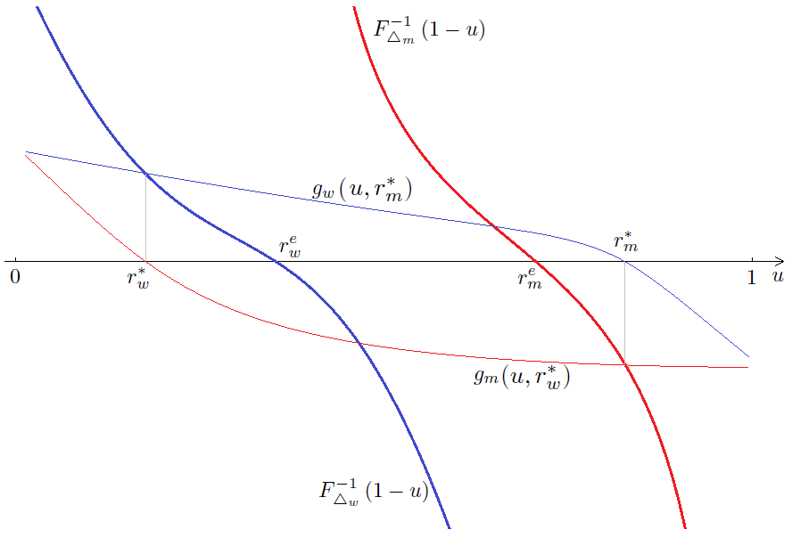
Figure 1. Illustration of the amplification of occupational segregation. The bright blue (resp. red) line traces the quantile function of type $\displaystyle w$ (resp. type $\displaystyle m$) sector $\displaystyle 1$ advantage. Fraction $\displaystyle r^{e}_{w}$ (resp. $\displaystyle r^{e}_{m}$) is the fraction of type $\displaystyle w$ (resp. type $\displaystyle m$) individuals in sector $\displaystyle 1$ in a Roy model with no composition effects. With composition effects, mediated by the $\displaystyle g$ functions defined in (1.3), these fractions move to $\displaystyle r^{*}_{w}$ and $\displaystyle r^{*}_{m}$.

Figure 1 gives a graphical illustration of the amplification effect of proposition 2. Efficient compositions $\displaystyle(r^{e}_{w},r^{e}_{m})$ (see definition 2) are replaced by more uneven equilibrium compositions $\displaystyle(r^{*}_{w},r^{*}_{m})$ as individuals respond to composition preferences. For instance, $\displaystyle g_{w}(u,r_{m}^{*})=g_{w}(u,r_{m}^{*},1/r)$ is the non pecuniary gain of a type $\displaystyle w$ individual from switching to sector $\displaystyle 2$ when the fraction of type $\displaystyle w$ individuals who choose sector $\displaystyle 1$ is $\displaystyle u$, and the fraction of type $\displaystyle m$ individuals who choose sector $\displaystyle 1$ is $\displaystyle r_{m}^{*}$.

1.5. Multiple equilibria and stability

Composition preferences compete with pecuniary incentives in a way that can lead to uneven compositions even when both types have identical primitive potential income distributions and identical preferences. Suppose both types have identical mass $\displaystyle\mu_{w}=\mu_{m}$ and identical sector $\displaystyle 1$ advantage, i.e., $\displaystyle F_{\Delta_{w}}=F_{\Delta_{m}}:=F_{\Delta}$. Hence, efficient compositions are also equal, i.e., $\displaystyle r^{e}_{w}=r^{e}_{m}:=r^{e}$. Suppose also that both types also have identical composition preferences.

In such a configuration, composition $\displaystyle(r^{e},r^{e})$ is an equilibrium. However, it is not stable if the slope of $\displaystyle g$ is steeper than the slope of $\displaystyle F_{\Delta}^{-1}$ at that point. Indeed, a small mass of type $\displaystyle w$ individuals switching from sector $\displaystyle 1$ to sector $\displaystyle 2$ would result in incentives for more type $\displaystyle w$ individuals to switch to sector $\displaystyle 2$ and for type $\displaystyle m$ individuals to switch to sector $\displaystyle 1$.

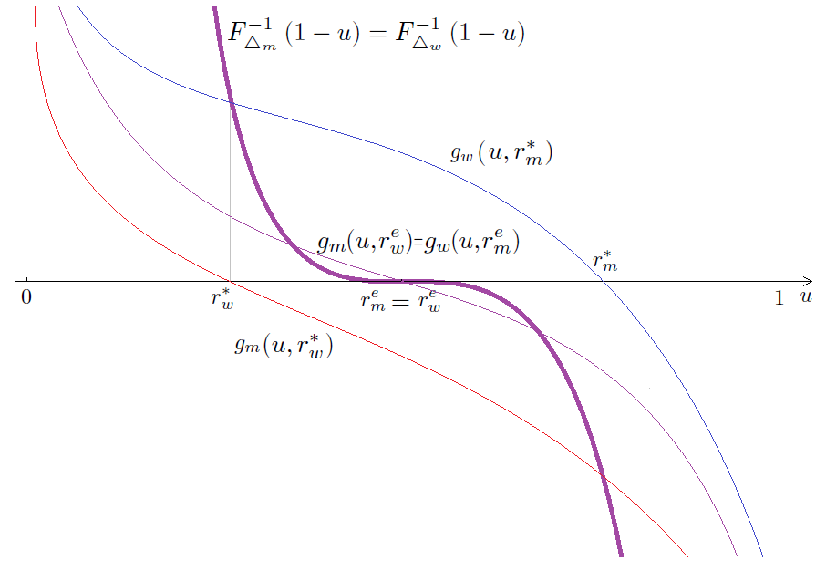
Figure 2. Illustration of purely endogenous composition imbalances. Both types have identical potential incomes and preferences. The slope of the composition preference effect $\displaystyle g$ is steeper at fraction $\displaystyle r^{e}$ than the slope of the quantile function $\displaystyle F^{-1}_{\Delta}$. The parity equilibrium composition $\displaystyle(r^{e},r^{e})$ is unstable, whereas the equilibrium $\displaystyle(r_{w}^{*},r_{m}^{*})$ with unbalanced type compositions is stable.

Figure 2 illustrates this situation, where the parity equilibrium is unstable, whereas the equilibrium with compositions $\displaystyle(r^{*}_{w},r^{*}_{m})$ is stable. Despite both groups being identical in preference and potential incomes, and despite no sector being favored a priori, composition preferences push the population to uneven compositions in both sectors.

2. Occupational segregation, redistribution and tipping effects

2.1. Parametric model specifications

To analyze the effects of redistribution and affirmative action in this model, we choose parametric specifications for the distributions of sector $\displaystyle 1$ advantage $\displaystyle\Delta_{t}=Y_{1t}-Y_{2t}$, $\displaystyle t\in\{w,m\}$, and for the composition preference functions $\displaystyle h_{w}$ and $\displaystyle h_{m}$.

Assumption 2.

There are parameters $\displaystyle r_{t}^{e}\in(0,1)$, $\displaystyle(c_{t},C_{t})\in\mathbb{R}_{+}^{2}$ and $\displaystyle\beta>0$ such that the composition preference function $\displaystyle h_{t}$ and the cumulative distribution function $\displaystyle F_{\Delta_{t}}$ of type $\displaystyle t$ sector $\displaystyle 1$ advantage $\displaystyle\Delta_{t}=Y_{1t}-Y_{2t}$ satisfy, for each $\displaystyle u\in(0,1)$ and for $\displaystyle t\in\{w,m\}$,

$$\displaystyle h_{t}(u)=\frac{c_{t}}{u}\;\mbox{ and }\;F_{\Delta_{t}}^{-1}(1-u)=C_{t}\frac{r_{t}^{e}-u}{[u(1-u)]^{\beta}}.$$

The location of the distribution of sector $\displaystyle 1$ advantage $\displaystyle\Delta_{t}=Y_{1t}-Y_{2t}$ is governed by $\displaystyle r_{t}^{e}$. The latter is the efficient composition of definition 2, i.e., the proportion of type $\displaystyle t$ individuals choosing sector $\displaystyle 1$ in a Roy model without composition effects. The scale of the distribution of sector $\displaystyle 1$ advantage is governed by $\displaystyle C_{t}$. Larger values of $\displaystyle C_{t}$ correspond to greater heterogeneity in sector $\displaystyle 1$ advantage among type $\displaystyle t$ individuals. The preference for composition is hyperbolic, which is intended to model strong aversion to being in a small minority. The aversion increases with larger values of the parameter $\displaystyle c_{t}$. Hence, the ratio $\displaystyle c_{t}/C_{t}$ measures the relative importance of pecuniary and composition considerations in choice.

Parameter $\displaystyle\beta$ governs the thickness of the tails of the distribution of sector $\displaystyle 1$ advantage. When $\displaystyle 0<\beta<1$, the tails of the distribution of sector $\displaystyle 1$ advantage are not fat enough to counteract aversion for being in a small minority, so that some full segregation of a group can be an equilibrium. If $\displaystyle\beta>1$, the tails of the distribution of sector $\displaystyle 1$ advantage are fat enough to counteract aversion for being in a small minority, so that some full segregation is not an equilibrium. The case $\displaystyle\beta=1$ yields closed form solutions for equilibrium compositions, as detailed in the next subsection.

2.2. Occupational segregation and redistribution

Stable equilibrium configurations depend on the relative importance of pecuniary and composition considerations in choice. We use parameters $\displaystyle\gamma_{t}$, $\displaystyle t\in\{w,m\}$ to gauge this relative importance, with

$$\displaystyle\begin{array}[]{lll}\gamma_{w}:=\frac{\mu_{m}}{\mu_{w}}\frac{c_{w}}{C_{w}}&\mbox{and}&\gamma_{m}:=\frac{\mu_{w}}{\mu_{m}}\frac{c_{m}}{C_{m}}.\end{array}$$ (2.2)

When both $\displaystyle\gamma_{w}$ and $\displaystyle\gamma_{m}$ are sufficiently small, the pecuniary incentive is sufficiently strong to guarantee existence of equilibrium with interior compositions, i.e., $\displaystyle r_{w}$ and $\displaystyle r_{m}$ both in $\displaystyle(0,1)$. If $\displaystyle\gamma_{w}$ or $\displaystyle\gamma_{m}$ is large enough, composition preferences push the equilibrium to a corner, where at least one type is confined to a single sector.

Proposition 3.

Under assumption 2 with $\displaystyle\beta=1$, if $\displaystyle 0<r_{w}^{e}<r_{m}^{e}<1$ and $\displaystyle\gamma_{w}+\gamma_{m}<1$, there is a unique equilibrium.

1. If $\displaystyle\bar{\gamma}:=\max\left\{\gamma_{w}r_{m}^{e}/r_{w}^{e}+\gamma_{m},\gamma_{w}+\gamma_{m}(1-r_{w}^{e})/(1-r_{m}^{e})\right\}<1,$ the unique equilibrium compositions $\displaystyle(r_{w}^{*},r_{m}^{*})$ are given by

   $$\displaystyle\begin{array}[]{lll}r_{w}^{*}&=&r_{w}^{e}-\frac{\gamma_{w}}{1-\gamma_{w}-\gamma_{m}}(r_{m}^{e}-r_{w}^{e}),\\ \\ r_{m}^{*}&=&r_{m}^{e}+\frac{\gamma_{m}}{1-\gamma_{w}-\gamma_{m}}(r_{m}^{e}-r_{w}^{e}).\end{array}$$ (2.6)

2. If $\displaystyle\gamma_{w}r_{m}^{e}/r_{w}^{e}+\gamma_{m}\geq 1$ and $\displaystyle\gamma_{m}<1-r_{m}^{e}$, the unique equilibrium compositions are $\displaystyle r_{w}^{*}=0$ and $\displaystyle r_{m}^{*}=r_{m}^{e}/(1-\gamma_{m})$.

3. If $\displaystyle\gamma_{w}<r_{w}^{e}$ and $\displaystyle\gamma_{w}+\gamma_{m}(1-r_{w}^{e})/(1-r_{m}^{e})\geq 1$, the unique equilibrium compositions are $\displaystyle r_{w}^{*}=(r_{w}^{e}-\gamma_{w})/(1-\gamma_{w})$ and $\displaystyle r_{m}^{*}=1$.

4. If $\displaystyle\gamma_{w}\geq r_{w}^{e}$ and $\displaystyle\gamma_{m}\geq 1-r_{m}^{e}$, the unique equilibrium compositions are $\displaystyle r_{w}^{*}=0$ and $\displaystyle r_{m}^{*}=1$.

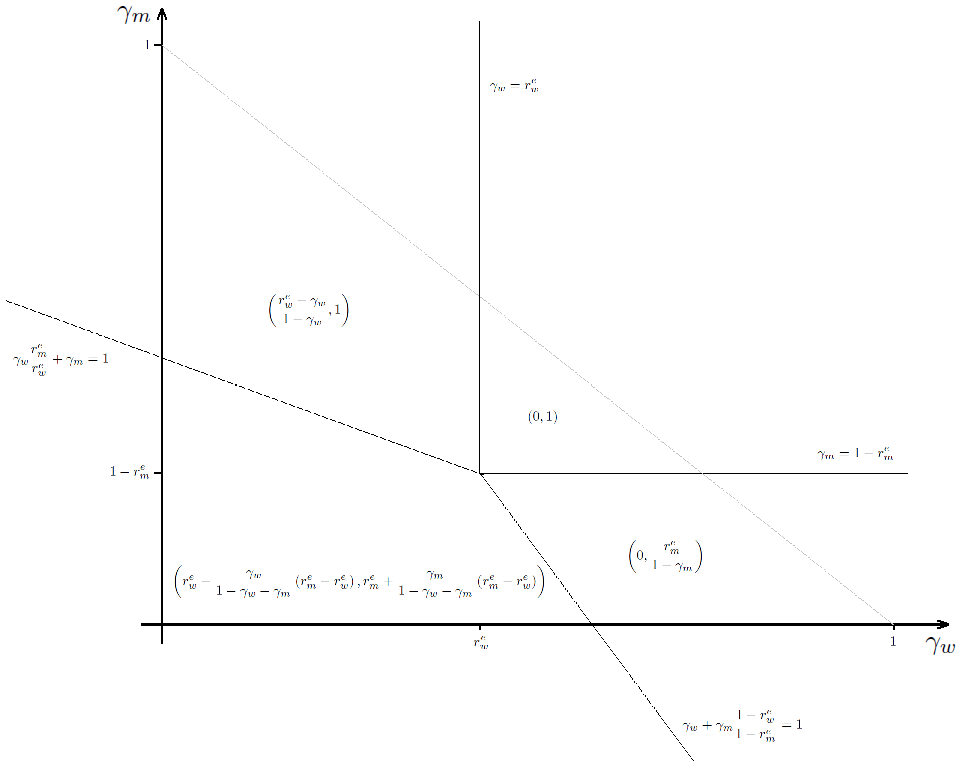
Figure 3. Illustration of the four equilibrium regions for $\displaystyle\gamma_{w}+\gamma_{m}<1$. In each region, the equilibrium described in proposition 3 is given in the form $\displaystyle(r_{w}^{*},r_{m}^{*})$.

The four equilibrium regions in the $\displaystyle(\gamma_{w},\gamma_{m})$ space are depicted in figure 3. The amplification effect of proposition 2 is quantified in proposition 3(1). Occupational segregation increases with the strength $\displaystyle\gamma_{t}$ of both types’ composition preferences relative to pecuniary incentives. Occupational segregation also increases with the primitive mean difference $\displaystyle r_{m}^{e}-r_{w}^{e}$ between type $\displaystyle m$ and type $\displaystyle w$ sector $\displaystyle 1$ advantage.

A tension arises between wealth redistribution and the reduction of occupational segregation. In general, anticipated redistribution reduces sector $\displaystyle 1$ advantage, hence the strength of pecuniary incentives relative to composition preferences. Specifically, a flat tax at rate $\displaystyle\tau$ redistributed equally affects sector choice by shrinking sector $\displaystyle 1$ advantage $\displaystyle\Delta_{t}$ to $\displaystyle(1-\tau)\Delta_{t}$. Hence, the effect of redistribution through a flat tax on occupational segregation is equivalent to a proportional increase of the strength $\displaystyle\gamma_{t}$ of composition preferences relative to pecuniary incentives to $\displaystyle\gamma_{t}/(1-\tau)$. This results in increased occupational segregation. If $\displaystyle\bar{\gamma}<1-\tau$, after redistribution, the equilibrium compositions $\displaystyle(r_{w}^{\tau},r_{m}^{\tau})$ are

$$\displaystyle\begin{array}[]{lllll}r_{w}^{\tau}&=&r_{w}^{e}-\frac{(1-\tau)\gamma_{w}}{1-(1-\tau)(\gamma_{w}+\gamma_{m})}(r_{m}^{e}-r_{w}^{e})&<&r_{w}^{*},\\ \\ r_{m}^{\tau}&=&r_{m}^{e}+\frac{(1-\tau)\gamma_{m}}{1-(1-\tau)(\gamma_{w}+\gamma_{m})}(r_{m}^{e}-r_{w}^{e})&>&r_{m}^{*}.\end{array}$$

If, however, $\displaystyle\bar{\gamma}\geq 1-\tau$, the effect of redistribution is to push compositions into a corner solution, where at least one type is confined to a single sector. For instance, if $\displaystyle\gamma_{w}r_{m}^{e}/r_{w}^{e}+\gamma_{m}\geq 1-\tau$ and $\displaystyle\gamma_{w}\geq r_{w}^{e}(1-\tau)$, type $\displaystyle w$ individuals will all switch to sector $\displaystyle 2$ as a result of redistribution.

The amplification of occupational segregation as a result of redistribution described in this section is one possible mechanism to explain the positive correlation between Gini index and the proportion of women among STEM graduates in the European Union, seen in figure 4, based on UNESCO’s UIS statistics (STEM shares) and World Bank indicators (GINI indices).

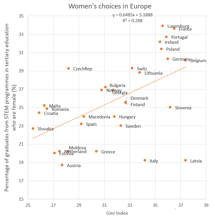
Figure 4. Regression of the proportion of women among STEM graduates (UIS data) against the Gini index of countries of the European Union (World Bank indicators).

2.3. Tipping and affirmative action

The Roy model with composition preferences displays tipping phenomena of two kinds. One type of tipping effect occurs when a small deviation in $\displaystyle(r_{w},r_{m})$ from one equilibrium tips the system to a different equilibrium. The second type of tipping effect occurs when the set of equilibria changes abruptly as the parameters $\displaystyle(\gamma_{w},\gamma_{m})$ that govern the relative strength of pecuniary and non pecuniary incentives cross a threshold. Unlike residential tipping in the work of Schelling (1971; 1973; 1978), tipping in this model is beneficial and occurs from highly segregated states to more even ones. Each type of tipping in this model is associated with a type of policy. Tipping as a shift between equilibrium is triggered by policies operating directly on compositions, such as quotas. Tipping as a change in the set of equilibria is triggered by policies operating on preferences or incomes, such as subsidies or changes in amenities, or changes in labor force participation.

2.3.1. Quotas and tipping

To analyze tipping between two equilibria, we consider the dynamical system induced by the Roy model with composition preferences. Consider type $\displaystyle w$ individuals for instance. If $\displaystyle\mu_{1w}/\mu_{w}>\mbox{Pr}\left[Y_{1w}-h_{w}\left(\mu_{1w}/\mu_{1}\right)>Y_{2w}-h_{w}\left(\mu_{2w}/\mu_{2}\right)\right],$ or, equivalently, if $\displaystyle r_{w}>F^{-1}_{\Delta_{w}}(1-r_{w})-g_{w}(r_{w},r_{m},r)$, the system is not in equilibrium, and a part of the type $\displaystyle w$ population is induced to move from sector $\displaystyle 1$ to sector $\displaystyle 2$. This also affects type $\displaystyle m$ individuals, so that movements of both types of individuals have to be considered jointly. Formally, the dynamical system is given by

$$\displaystyle\begin{array}[]{lll}\dot{r}_{w}&=&F^{-1}_{\Delta_{w}}(1-r_{w})-g_{w}(r_{w},r_{m},r),\\ \\ \dot{r}_{m}&=&F^{-1}_{\Delta_{m}}(1-r_{m})-g_{w}(r_{m},r_{w},1/r),\end{array}$$ (2.11)

where $\displaystyle\dot{r}$ indicates the time derivative of $\displaystyle r$. Figure 5 is a phase diagram for this dynamical system in the case of $\displaystyle\beta=0.05$ in assumption 2 and specific values for the efficient compositions $\displaystyle r^{e}_{w}$ and $\displaystyle r^{e}_{m}$ and the relative strength $\displaystyle(\gamma_{w},\gamma_{m})$ of pecuniary and non pecuniary incentives. Blue curves are the loci of $\displaystyle F^{-1}_{\Delta_{w}}(1-r_{w})=g_{w}(r_{w},r_{m},r)$ and $\displaystyle F^{-1}_{\Delta_{m}}(1-r_{m})=g_{w}(r_{m},r_{w},1/r)$. Black arrows indicate the direction of change in $\displaystyle(r_{w},r_{m})$ off equilibrium. Black (resp. red) dots indicate unstable (resp. stable) equilibria.

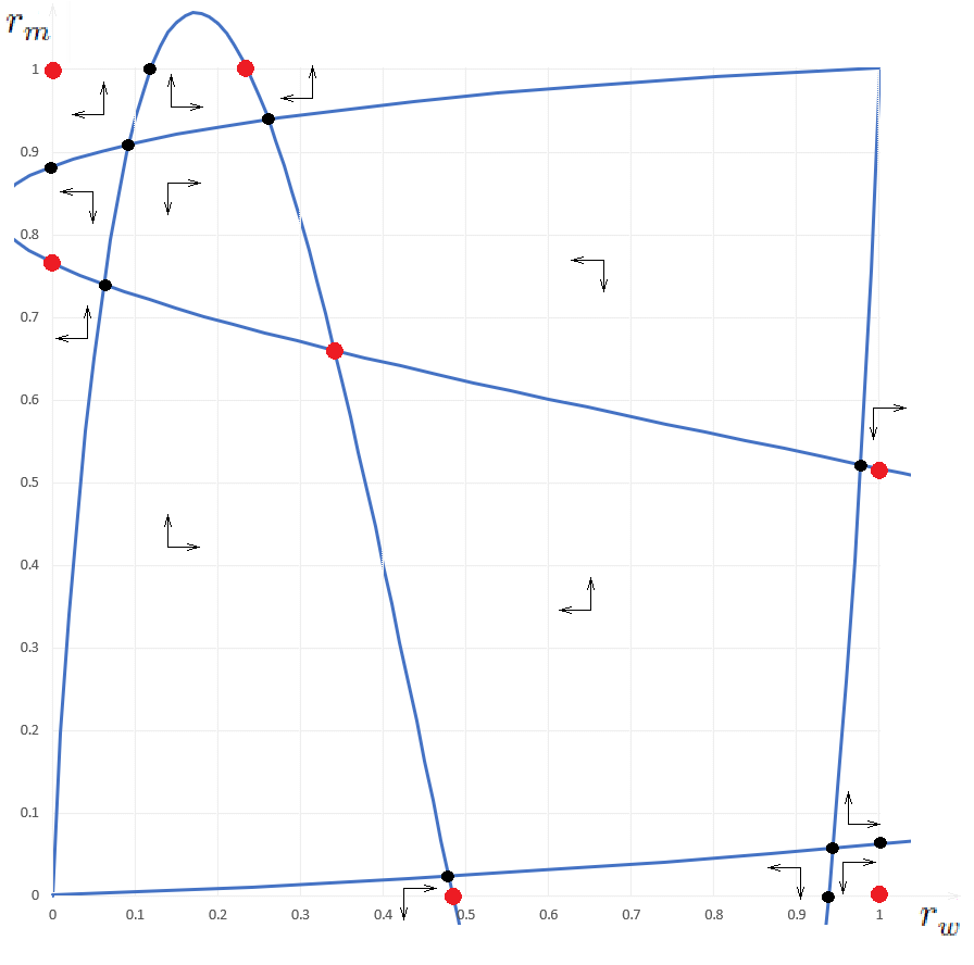
Figure 5. Phase diagram for dynamical system (2.11) with $\displaystyle\beta=0.05,\gamma_{w}=\gamma_{m}=0.11$, $\displaystyle r^{e}_{w}=0.4$ and $\displaystyle r^{e}_{m}=0.6$. There are $\displaystyle 17$ equilibria, $\displaystyle 7$ of which are stable (in red), including $\displaystyle 6$ corner and $\displaystyle 1$ interior equilibrium. Black arrows indicate the direction of attraction of the differential system. Tipping occurs when a small deviation from any of the stable corner equilibria pushes the system to the domain of attraction of the interior equilibrium.

Holding parameters $\displaystyle(r^{e}_{w},r^{e}_{m})$ and $\displaystyle(\gamma_{w},\gamma_{m})$ fixed, hence holding both sector 1 advantage and preferences fixed for both types, a quota of $\displaystyle 10\%$ for the representation of each type in each sector pushes the dynamical system from any of the corner equilibria to the unique interior equilibrium $\displaystyle(r^{*}_{w},r^{*}_{m})$. The latter displays the amplification feature uncovered in proposition 2, i.e., $\displaystyle r^{*}_{w}<r^{e}_{w}<r^{e}_{m}<r^{*}_{m}$. However, given the modest composition preferences relative to pecuniary incentives (low values of parameters $\displaystyle\gamma_{w}$ and $\displaystyle\gamma_{m}$), this amplification effect is small.

2.3.2. Subsidies, change in amenities and tipping

The quota policy entertained in section 2.3.1 operates through a change in compositions $\displaystyle(r_{w},r_{m})$ while keeping the distribution $\displaystyle F_{\Delta}$ of sector $\displaystyle 1$ advantage and preferences $\displaystyle h_{t}$ fixed, $\displaystyle t\in\{w,m\}$. In contrast, subsidies operate on $\displaystyle F_{\Delta}$, and amenity changes operate on composition preferences $\displaystyle h_{t}$ without affecting compositions directly. Consider a class of policies that reduce parameters $\displaystyle\gamma_{w}$ and $\displaystyle\gamma_{m}$. They can provoke tipping through the disappearance of a contrarian equilibrium, i.e., a corner equilibrium which excludes from a given sector the type that enjoys a comparative advantage in that sector.

We describe an example of contrarian equilibrium in the case of $\displaystyle\beta=1$ in assumption 2. Let $\displaystyle r^{e}_{w}>r^{e}_{m}$ so that type $\displaystyle w$ has an advantage in sector $\displaystyle 1$. Suppose also that $\displaystyle\gamma_{w}r^{e}_{m}>(1-\gamma_{m})r^{e}_{w}$ and $\displaystyle\gamma_{m}<1-r_{m}^{e}$, so that type $\displaystyle w$ has stronger composition preferences than type $\displaystyle m$. Then, $\displaystyle(r^{*}_{w}=0,r^{*}_{m}=r^{e}_{m}/(1-\gamma_{m}))$ is a stable equilibrium. Indeed,

$$\lim_{r_{w}\downarrow 0}\frac{F^{-1}_{\Delta_{w}}(1-r_{w})}{g_{w}(r_{w},r_{m}^{*},r)}=\frac{1-\gamma_{m}}{\gamma_{w}}\frac{r^{e}_{w}}{r^{e}_{m}}\leq 0,$$

so no small mass of type $\displaystyle w$ individuals has an incentive to move to sector $\displaystyle 1$, nor would a small deviation create such an incentive. Moreover, $\displaystyle F^{-1}_{\Delta_{m}}(1-r_{m}^{*})=g_{m}(r^{*}_{m},0,1/r)$ so that no small mass of type $\displaystyle m$ individuals have an incentive to switch. Finally, small deviations do not create incentives for type $\displaystyle m$ individuals to switch since $\displaystyle dF^{-1}_{\Delta_{m}}(1-r_{m}^{*})/dr_{m}<\partial g_{m}(r^{*}_{m},0,1/r)/\partial r_{m}$. Tipping occurs when parameters $\displaystyle(\gamma_{w},\gamma_{m})$ decrease beyond the threshold defined by $\displaystyle\gamma_{w}r^{e}_{m}=(1-\gamma_{m})r^{e}_{w}$. When $\displaystyle\gamma_{w}r^{e}_{m}<(1-\gamma_{m})r^{e}_{w}$, the contrarian equilibrium disappears.

2.3.3. Rise in labor force participation and tipping

The model also exhibits another type of tipping, through the disappearance of a weakly contrarian interior equilibrium. In figure 6, a rise in type $\displaystyle w$ labor participation leads to the disappearance of an equilibrium. We call this equilibrium weakly contrarian because type $\displaystyle w$ has comparative advantage in sector 1, i.e., $\displaystyle(r_{w}^{e}>r_{m}^{e})$, but the equilibrium is such that $\displaystyle r_{w}^{*}<r_{m}^{*}$. When the weakly contrarian equilibrium disappears as type $\displaystyle w$ labor force participation increases, the only remaining equilibrium is an interior equilibrium that reflects type $\displaystyle w$’s comparative advantage in sector $\displaystyle 1$, i.e., such that $\displaystyle r_{w}^{*}>r_{m}^{*}$. This provides an alternative mechanism for the rapid shifts in gender compositions for occupations such as bankers and insurance agents documented in Pan (2015).

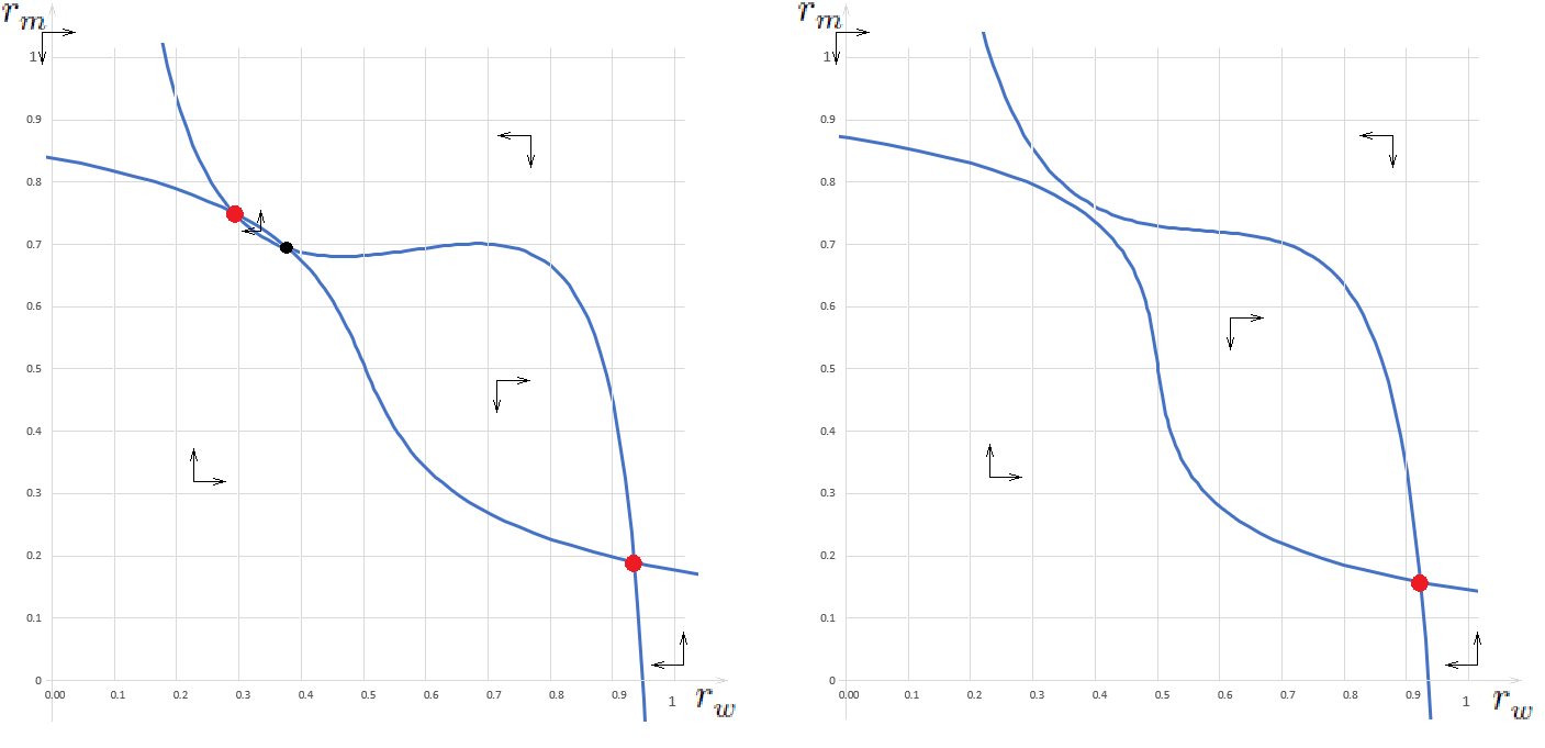
Figure 6. Phase diagrams for dynamical system (2.11) with $\displaystyle\beta=2,c_{w}=c_{m}=3.5,C_{w}=C_{m}=1,\mu_{m}=1,r_{w}^{e}=0.7$ and $\displaystyle r_{m}^{e}=0.5$. The two diagrams are differ in $\displaystyle\mu_{w}$. On the left diagram $\displaystyle\mu_{w}=0.8$, on the right diagram $\displaystyle\mu_{w}=1$. So an increase of type $\displaystyle w$ labor force participation leads to the disappearance of a weakly contrarian equilibrium.

3. Empirical content of the Roy model with composition effects

3.1. Empirical model

We propose the following empirical version of the Roy model with composition preferences. Individual $\displaystyle i$ with type $\displaystyle t_{i}\in\{w,m\}$ chooses sector $\displaystyle 1$, denoted by $\displaystyle D_{i}=1$ if $\displaystyle\Delta_{i}>g_{t_{i}}+\xi_{i}$, where $\displaystyle\Delta_{i}=Y_{1i}-Y_{2i}$, $\displaystyle g_{t_{i}}:=g_{w}(r_{w},r_{m},1/r)$ if $\displaystyle t_{i}=w$, and $\displaystyle g_{t_{i}}:=g_{m}(r_{m},r_{w},r)$ if $\displaystyle t_{i}=m$, and $\displaystyle\xi_{i}$ is a random variable with cumulative distribution function $\displaystyle F_{\xi}$, independent of $\displaystyle\Delta_{i}$. Individual $\displaystyle i$ chooses sector $\displaystyle 2$ otherwise, denoted by $\displaystyle D_{i}=2$. We interpret this choice model as the result of utility maximization as in section 1.2, where the utility includes an additive sector specific random utility term. Finally let $\displaystyle\underline{w}\geq 0$ be the minimum wage and assume that the support of all income distributions is bounded below by $\displaystyle\underline{w}$.

Individual $\displaystyle i$’s realized income is $\displaystyle Y_{i}=Y_{1i}$ when $\displaystyle D_{i}=1$ and $\displaystyle Y_{2i}$ when $\displaystyle D_{i}=2$. We assume that the four distributions of realized incomes for each type and each sector are observed in the population. Hence, the quantities $\displaystyle\mbox{Pr}(Y_{i}\leq y,D_{i}=d,t_{i}=t)$ are assumed known for all $\displaystyle t\in\{w,m\}$, $\displaystyle d\in\{0,1\}$, and $\displaystyle y\geq\underline{w}$. Type sector compositions $\displaystyle(r^{*}_{w},r^{*}_{m})$ are observed. They are assumed to be equilibrium compositions. The ratio $\displaystyle r$ of total populations of both types is also observed. The cumulative distribution function $\displaystyle F_{\xi}$ of the random utility term is assumed known. The minimum wage $\displaystyle\underline{w}$ is also assumed known.

3.2. Sharp bounds on the primitives

The distribution of potential incomes is not observed and cannot be directly estimated, since income is only observed in the chosen sector. Therefore, the vector of parameters is not point identified in general. We provide a sharp characterization of the identified set, i.e., the set of parameter values that cannot be rejected on the basis of the decision model and the observed choices and realized incomes.

Start with simple implications of the model. Take individual $\displaystyle i$ with type $\displaystyle t_{i}$, potential incomes $\displaystyle(Y_{1i},Y_{2i})$, sector $\displaystyle 1$ advantage $\displaystyle\Delta_{i}$, and realized income $\displaystyle Y_{i}$. Suppose individual $\displaystyle i$ is in sector $\displaystyle 1$ and has a realized income that is smaller than $\displaystyle y$, for some $\displaystyle y\geq\underline{w}$. Individual $\displaystyle i$’s sector advantage $\displaystyle\Delta_{i}=Y_{1i}-Y_{2i}$ must then be smaller than $\displaystyle y-\underline{w}$, since $\displaystyle Y_{1i}=Y_{i}\leq y$ and $\displaystyle Y_{2i}\geq\underline{w}$. Moreover, by the choice model, $\displaystyle D_{i}=1$ also implies $\displaystyle\Delta_{i}>g_{t_{i}}^{*}+\xi_{i}$, where $\displaystyle g_{t_{i}}^{*}:=g_{w}(r_{w}^{*},r_{m}^{*},r)$ if $\displaystyle t_{i}=w$ and $\displaystyle g_{t_{i}}^{*}:=g_{m}(r_{m}^{*},r_{w}^{*},1/r)$ if $\displaystyle t_{i}=m$. Hence, we obtain, for all $\displaystyle y\geq\underline{w}$, the implication $\displaystyle\mbox{Pr}(g_{t_{i}}^{*}+\xi_{i}<\Delta_{i}\leq y-\underline{w},t_{i}=t)\geq\mbox{Pr}(Y_{i}\leq y,D_{i}=1,t_{i}=t)$, which gives a bound on the unknown distribution of individual $\displaystyle i$’s sector $\displaystyle 1$ advantage $\displaystyle\Delta_{i}$. Since the random utility component $\displaystyle\xi_{i}$ is independent of $\displaystyle\Delta_{i}$, and its distribution is known, the bound can be integrated over $\displaystyle\xi_{i}$ to yield

$$\displaystyle\begin{array}[]{lll}\int\mbox{Pr}(g_{t_{i}}^{*}+\xi<\Delta_{i}\leq y-\underline{w},t_{i}=t)dF_{\xi}(\xi)&\geq&\mbox{Pr}(Y_{i}\leq y,D_{i}=1,t_{i}=t).\end{array}$$ (3.2)

The same reasoning applies to the case $\displaystyle Y_{i}>y$ and $\displaystyle D_{i}=2$ to yield the bound

$$\displaystyle\begin{array}[]{lll}\int\mbox{Pr}(\underline{w}-y<\Delta_{i}\leq g_{t_{i}}^{*}+\xi,t_{i}=t)dF_{\xi}(\xi)&\geq&\mbox{Pr}(Y_{i}>y,D_{i}=0,t_{i}=t),\end{array}$$ (3.4)

for all $\displaystyle y\geq\underline{w}$, $\displaystyle t\in\{w,m\}$.

3.3. Inference on structural parameters and counterfactual analysis

When potential incomes and composition preferences satisfy assumption 2, system (3.2)-(3.4) defines a continuum of moment inequalities. For each $\displaystyle y\geq\underline{w}$, and each value of the parameter vector $\displaystyle(r^{e}_{w},r^{e}_{m},c_{w},c_{m},C_{w},C_{m})$, the moment inequalities can be evaluated numerically, and confidence regions derived using existing inference methods on moment inequality models (see for instance Canay and Shaihk (2017) for a survey).

Once structural parameters are recovered, we can evaluate the effect of policies described in sections 2.3.1 and 2.3.2 in the following way. Given the parameter values and the observed equilibrium compositions, the phase diagram for the dynamical system (2.11) determines the equilibrium that would result from the imposition of a quota system, holding structural parameters fixed. In the case of a policy that shifts the parameters $\displaystyle C_{t}$ (a subsidy) of $\displaystyle c_{t}$ (an exogenous change in workplace culture), the new parameter values determine a new phase diagram for the dynamical system (2.11), which also determines the resulting equilibrium.

4. Discussion

We proposed a model combining comparative advantage with composition preferences in labor market sector selection. This allowed us to propose one mechanism to explain high levels of occupational segregation as well as the observed counterintuitive negative correlation between inequality and gender occupational segregation. The model could easily be extended to accommodate preference for parity, where the disutility function increases on either side of parity. This could be interpreted as a tradeoff between homophily and marriage market considerations. Group identity (Akerlof and Kranton (2000), Bertrand et al. (2015), Bertrand (2011)), operates through human capital accumulation, but also compositions. For instance, a small ratio of women reinforces the gendered perception of an occupation. Mentoring in the career development of women operates through potential incomes, as lifetime earnings are affected, but it could be incorporated in a multi generation version of the model).

However, the sharp separation between comparative advantage, whose effect on self-selection is mediated through potential incomes, and nonpecuniary drivers of selection, mediated through compositions and social effects, brings with it some major limitations. One major limitation of the model is that composition effects on learning are ruled out. Potential incomes (that incorporate human capital accumulation) are unaffected by type-sector compositions. Peer effects are limited to non pecuniary benefits and cannot affect future productivity. The model also rules out effects of gender compositions on the gender wage gap, through realistic channels such as increased wage discrimination in STEM fields because of low representation of women. The model is a full information game, so that gender specific bias in wage expectations is ruled out as a factor in under-representation of women in STEM. It is also frictionless, so there is no place for job search strategies, homophily in referral networks, as in Fernandez and Sosa (2005), Zelzer (2020) and Buhai and van der Leij (2020).

Appendix A Proofs of results in the main text

We prove proposition 2 first, then proposition 1, which relies on proposition 2, and finally proposition 3.

A.1. Proof of proposition 2

First, note that, under assumption 1, the function $\displaystyle g_{t}(x,y,z)$ defined in (1.3) for $\displaystyle t\in\{w,m\}$ is decreasing in $\displaystyle x$ and increasing in $\displaystyle y$ and satisfies $\displaystyle g_{t}(x,x,z)=0$ for all $\displaystyle(x,y,z)\in(0,1)^{3}$. Next, we construct a non increasing sequence $\displaystyle(r_{w}^{(l)})_{l\in\mathbb{N}}$, and a non decreasing sequence $\displaystyle(r_{m}^{(l)})_{l\in\mathbb{N}}$, in the following way. Define $\displaystyle r_{w}^{(1)}:=r_{w}^{e}$ and $\displaystyle r_{m}^{(1)}:=r_{m}^{e}$. By definition of $\displaystyle(r_{w}^{e},r_{m}^{e})$, we have $\displaystyle F^{-1}_{\Delta_{w}}(1-r_{w}^{(1)})=F^{-1}_{\Delta_{m}}(1-r_{m}^{(1)})=0$. Moreover, since $\displaystyle r_{w}^{(1)}=r_{w}^{e}<r_{m}^{e}=r_{m}^{(1)}$ by assumption, the properties of functions $\displaystyle g_{t}$, $\displaystyle t\in\{w,m\}$, noted above imply that

$$g_{m}(r_{m}^{(1)},r_{w}^{(1)},r)<0<g_{w}(r_{w}^{(1)},r_{m}^{(1)},1/r).$$

Hence,

$$\displaystyle F_{\Delta_{w}}(g_{w}(r_{w}^{(1)},r_{m}^{(1)},1/r))>F_{\Delta_{w}}(0)=1-r_{w}^{(1)} \displaystyle F_{\Delta_{w}}(g_{w}(0,r_{m}^{(1)},1/r))\leq 1,$$ and

$$\displaystyle F_{\Delta_{m}}(g_{m}(r_{m}^{(1)},r_{w}^{(1)},r))<F_{\Delta_{m}}(0)=1-r_{m}^{(1)} \displaystyle F_{\Delta_{m}}(g_{m}(1,r_{w}^{(1)},r))\geq 0.$$ and

Now assume $\displaystyle(r_{w}^{(l)},r_{m}^{(l)})$ are defined in such a way that

$$\displaystyle F_{\Delta_{w}}(g_{w}(r_{w}^{(l)},r_{m}^{(l)},1/r))>1-r_{w}^{(l)} \displaystyle F_{\Delta_{w}}(g_{w}(0,r_{m}^{(l)},1/r))\leq 1,$$ and

$$\displaystyle F_{\Delta_{m}}(g_{m}(r_{m}^{(l)},r_{w}^{(l)},r))<1-r_{m}^{(l)} \displaystyle F_{\Delta_{m}}(g_{m}(1,r_{w}^{(l)},r))\geq 0.$$ and

Under assumption 1, functions $\displaystyle F^{-1}_{\Delta_{t}}$ and $\displaystyle g_{t}$, $\displaystyle t\in\{w,m\}$, are continuous, so that there exist $\displaystyle(r_{w}^{(l+1)},r_{m}^{(l+1)})$ such that $\displaystyle 0\leq r_{w}^{(l+1)}<r_{w}^{(l)}$ and $\displaystyle r_{m}^{(l)}<r_{m}^{(l+1)}\leq 1$ satisfying

$$F^{-1}_{\Delta_{w}}(1-r_{w}^{(l+1)})=g_{w}(r_{w}^{(l+1)},r_{m}^{(l)},1/r)\mbox{ and }F^{-1}_{\Delta_{m}}(1-r_{m}^{(l+1)})=g_{m}(r_{m}^{(l+1)},r_{w}^{(l)},r).$$

Calling $\displaystyle r_{w}^{*}$ and $\displaystyle r_{m}^{*}$ the limits of the monotone sequences $\displaystyle(r_{w}^{(l)})$ and $\displaystyle(r_{m}^{(l)})$ on $\displaystyle[0,1]$, and passing to the limit yields the first result.

Assume now that there is an equilibrium $\displaystyle(r_{w}^{*},r_{m}^{*})$ such that $\displaystyle r_{w}^{e}<r_{w}^{*}<r_{m}^{*}<r_{m}^{e}$. Then $\displaystyle\Rightarrow g_{w}\left(r_{w}^{*},r_{m}^{*},1/r\right)<0$. Since $\displaystyle g_{w}\left(r_{w},r_{m},1/r\right)$ is decreasing in $\displaystyle r_{w}$ and $\displaystyle r_{w}^{*}<r_{m}^{*}$, we therefore have $\displaystyle g_{w}\left(r_{w}^{*},r_{m}^{*},1/r\right)\geq g_{w}\left(r_{m}^{*},r_{m}^{*},1/r\right)$. Hence, we find $\displaystyle g_{w}\left(r_{m}^{*},r_{m}^{*},1/r\right)<0$, which yields a contradiction, since we know that $\displaystyle g_{w}\left(r_{m}^{*},r_{m}^{*},1/r\right)=0$.

A.2. Proof of proposition 1

Existence of a solution to the system

$$\displaystyle\begin{array}[]{lll}F^{-1}_{\Delta_{w}}(1-r_{w})&=&\sigma g_{w}(r_{w},r_{m},1/r),\\ \\ F^{-1}_{\Delta_{m}}(1-r_{m})&=&\sigma g_{m}(r_{m},r_{w},r),\end{array}$$ (A.4)

is guaranteed by proposition 2 in the case $\displaystyle r_{w}^{e}<r_{m}^{e}$. In the case $\displaystyle r_{w}^{e}=r_{m}^{e}$, $\displaystyle(r_{w}^{e},r_{m}^{e})$ is a solution. To show uniqueness, we first show that for small enough $\displaystyle\sigma$, any solution is close to $\displaystyle(r_{w}^{e},r_{m}^{e})$. Fix $\displaystyle\varepsilon>0$. There is a $\displaystyle\delta>0$ such that $\displaystyle|u|<\delta$ implies

$$\max\{|1-r_{w}^{e}-F_{\Delta_{w}}(u)|,|1-r_{m}^{e}-F_{\Delta_{m}}(u)|\}<\varepsilon.$$

By continuity of $\displaystyle g_{t}$, $\displaystyle t\in\{w,m\}$, there is a $\displaystyle\sigma>0$ such that $\displaystyle\sigma\max\{g_{w}(r_{w},r_{m},1/r),g_{m}(r_{m},r_{w},r)\}<\delta$. Hence, for such a $\displaystyle\sigma$, any solution $\displaystyle(r_{w}^{*},r_{m}^{*})$ to (A.4) must satisfy

$$\displaystyle\max\{|r_{w}^{*}-r_{w}^{e}|,|r_{m}^{*}-r_{m}^{e}|\}<\varepsilon.$$ (A.5)

Let $\displaystyle(r_{m}^{*},r_{m}^{*})$ and $\displaystyle(\tilde{r}_{w},\tilde{r}_{m})$ be two distinct solutions of system (A.4). Then

$$\displaystyle F^{-1}_{\Delta_{w}}(1-r_{w}^{*})-F^{-1}_{\Delta_{w}}(1-\tilde{r}_{w})=\sigma\left[g_{w}(r_{w}^{*},r_{m}^{*},1/r)-g_{w}(\tilde{r}_{w},r_{m}^{*},1/r)+g_{w}(\tilde{r}_{w},r_{m}^{*},1/r)-g_{w}(\tilde{r}_{w},\tilde{r}_{m},1/r)\right].$$ (A.6)

Now, given (A.5),

$$\displaystyle F^{-1}_{\Delta_{w}}(1-r_{w}^{*})-F^{-1}_{\Delta_{w}}(1-\tilde{r}_{w})\geq|r_{w}^{*}-\tilde{r}_{w}|\inf_{|u-r_{w}^{e}|<\varepsilon}\left[-\frac{d}{du}F^{-1}_{\Delta_{w}}(1-u)\right],$$ (A.7)

and

$$\displaystyle\begin{array}[]{lll}|g_{w}(r_{w}^{*},r_{m}^{*},1/r)-g_{w}(\tilde{r}_{w},r_{m}^{*},1/r)|&\leq&|r_{w}^{*}-\tilde{r}_{w}|\sup_{|u-r_{w}^{e}|<\varepsilon}\left[\frac{\partial}{\partial r_{m}}g_{w}(r_{w},r_{m}^{*},1/r)\right],\\ \\ |g_{w}(\tilde{r}_{w},r_{m}^{*},1/r)-g_{w}(\tilde{r}_{w},\tilde{r}_{m},1/r)|&\leq&|r_{m}^{*}-\tilde{r}_{m}|\sup_{|u-r_{m}^{e}|<\varepsilon}\left[\frac{\partial}{\partial r_{m}}g_{m}(\tilde{r}_{w},r_{m},r)\right].\end{array}$$ (A.11)

Together, (A.6), (A.7) and (A.11) imply

$$\displaystyle|r_{w}^{*}-\tilde{r}_{w}|\leq\sigma\left(K_{1}|r_{w}^{*}-\tilde{r}_{w}|+K_{2}|r_{m}^{*}-\tilde{r}_{m}|\right).$$ (A.12)

for some $\displaystyle K_{1}>0$ and $\displaystyle K_{2}>0$. Similar expressions obtain for the second equation in system (A.4) to yield

$$\displaystyle|r_{m}^{*}-\tilde{r}_{m}|\leq\sigma\left(K_{3}|r_{w}^{*}-\tilde{r}_{w}|+K_{4}|r_{m}^{*}-\tilde{r}_{m}|\right),$$ (A.13)

for some $\displaystyle K_{3}>0$ and $\displaystyle K_{4}>0$. For $\displaystyle\sigma<\min(K_{1}^{-1},K_{2}^{-1},K_{3}^{-1},K_{4}^{-1})/2$, combining (A.12) and (A.13) yields a contradiction.

A.3. Proof of proposition 3

We prove proposition 3 by enumerating all types of equilibria that can arise under assumption 2 with $\displaystyle\gamma_{w}+\gamma_{m}<1$.

1. If $\displaystyle(r_{w}^{*},r_{m}^{*})$ is an interior equilibrium, i.e., $\displaystyle(r_{w}^{*},r_{m}^{*})\in(0,1)^{2}$, then it must solve system (1.1)-(1.2). Hence, $\displaystyle(r_{w}^{*},r_{m}^{*})$ must be given by $\displaystyle(\ref{eq:sol})$. In addition, for $\displaystyle(r_{w}^{*},r_{m}^{*})$ to be in $\displaystyle(0,1)^{2}$, we must have $\displaystyle\bar{\gamma}<1$. Conversely, if $\displaystyle\bar{\gamma}<1$ and $\displaystyle(r_{w}^{*},r_{m}^{*})$ is given by $\displaystyle(\ref{eq:sol})$, then it is an equilibrium.

2. For $\displaystyle(0,r_{m}^{*})$ to be an equilibrium, with $\displaystyle 0<r_{m}^{*}<1$, then $\displaystyle r_{m}^{*}$ must solve (1.2), which is equivalent to $\displaystyle r_{m}^{e}-r_{m}^{*}=\gamma_{m}(0-r_{m}^{*})$, and be in $\displaystyle(0,1)$, which yields $\displaystyle r_{m}^{*}=r_{m}^{e}/(1-\gamma_{m})$ and $\displaystyle\gamma_{m}<1-r_{m}^{e}$. Moreover, type $\displaystyle w$ individuals have no incentive to switch to sector $\displaystyle 1$, so that $\displaystyle\gamma_{w}r_{m}^{e}/r_{w}^{e}+\gamma_{m}\geq 1$.

Cases (3) and (4) are treated similarly. The remaining possible equilibrium configurations, with $\displaystyle r_{w}^{*}=1$ and $\displaystyle(r_{w}^{*},0)$, with $\displaystyle 0,r_{w}^{*}<1$, are shown to be incompatible with $\displaystyle\gamma_{w}+\gamma_{m}<1$.

References

- Akerlof and Kranton (2000) G. Akerlof and R. Kranton. Economics and identity. Quarterly Journal of Economics, 115:715–753, 2000.
- Arrow (1998) K. Arrow. What has economics to say about racial discrimination? Journal of Eco- nomic Perspectives, 12:91–100, 1998.
- Baumol (1990) W. Baumol. Entrepreneurship: productive, unproductive, and destructive. Journal of Political Economy, 98:893–921, 1990.
- Becker (1985) G. Becker. Human capital, effort, and the sexual division of labor. Journal of Labor Economics, 3:S33–S58, 1985.
- Bernheim (1994) D. Bernheim. A theory of conformity. Journal of Political Economy, 102:841–877, 1994.
- Bertrand (2011) M. Bertrand. New perspectives on gender. In O. Ashenfelter and D. Card, editors, Handbook of Labor Economics, volume 4b, pages 1543–1590. Elsevier, North-Holland, 2011.
- Bertrand et al. (2015) M. Bertrand, E. Kamenica, and J. Pan. Gender identity and relative income within households. Quarterly Journal of Economics, 130:571–614, 2015.
- Bertrand et al. (2019) M. Bertrand, S. Black, S. Jensen, and A. Lleras-Muney. Breaking the glass ceiling? the effect of board quotas on female labour market outcomes in Norway. Review of Economic Studies, 86:191–239, 2019.
- Blau and Kahn (2017) F. Blau and L. Kahn. The gender wage gap: Extent, trends, and explanations. Journal of Economic Literature, 55:789–865, 2017.
- Blonski (1999) M. Blonski. Anonymous games with binary actions. Games and Economic Behavior, 28:171–180, 1999.
- Bostwick and Weinberg (2021) V. Bostwick and B. Weinberg. Nevertheless she persisted? Gender peer effects in doctoral STEM programs. Journal of Labor Economics, forthcoming, 2021.
- Brock and Durlauf (2001) W. Brock and S. Durlauf. Discrete choice with social interactions. Review of Economic Studies, 68:235–260, 2001.
- Buffington et al. (2016) C. Buffington, B. Cerf, C. Jones, and B. Weinberg. STEM training and early career outcomes of female and male graduate students: Evidence from UMETRICS data linked to the 2010 census. American Economic Review, Papers and Proceedings, 106:333–338, 2016.
- Buhai and van der Leij (2020) S. Buhai and M. van der Leij. A social network analysis of occupational segregation. unpublished manuscript, 2020.
- Canay and Shaihk (2017) I. Canay and A. Shaihk. Practical and theoretical advances in inference for partially identified models. In B. Honoré, A. Pakes, M. Piazzesi, and L. Samuelson, editors, Advances in Economics and Econometrics: Eleventh World Congress, volume 2, pages 271–306. Cambridge University Press, 2017.
- Card et al. (2008) D. Card, A. Mas, and J. Rothstein. Tipping and the dynamics of segregation. Quaterly Journal of Economics, 123:177–218, 2008.
- Carlana (2019) M. Carlana. Implicit stereotypes: Evidence from teachers’ gender bias. Quarterly Journal of Economics, 134(1163–1224), 2019.
- Cooper and John (1988) R. Cooper and A. John. Coordinating coordination failures in keynesian models. Quarterly Journal of Economics, 103:441–463, 1988.
- Daymont and Andrisani (1984) T. N. Daymont and P. J. Andrisani. Job preferences, college major, and the gender gap in earnings. Journal of Human Resources, pages 408–428, 1984.
- Ellison and Fudenberg (2003) G. Ellison and D. Fudenberg. Knife-edge or plateau: When do market models tip? Quarterly Journal of Economics, 118:1249–1278, 2003.
- Ellison and Swanson (2010) G. Ellison and A. Swanson. The gender gap in secondary school mathematics at high achievement levels: Evidence from the american mathematics competitions. Journal of Economic Perspectives, 24:109–128, 2010.
- Fernandez and Sosa (2005) R. Fernandez and L. Sosa. Gendering the job: Networks and recruitment at a call center. American Journal of Sociology, 111:859–904, 2005.
- Fine et al. (2020) C. Fine, V. Sojo, and H. Lawford-Smith. Why does workplace gender diversity matter? justice, organizational benefits, and policy. Social Issues and Policy Review, 14:36–72, 2020.
- Glauber (2011) R. Glauber. Limited access: Gender, occupational composition, and flexible work scheduling. The Scociological Quarterly, 52:472–494, 2011.
- Gutek and Morasch (1982) B. Gutek and B. Morasch. Sex-ratios, sex-role spillover, and sexual harassment of women at work. Journal of Social Issues, 38:55–74, 1982.
- Heal and Kunreuther (2006) G. Heal and H. Kunreuther. Supermodularity and tipping. NBER Working Paper No. 12281, 2006.
- Heckman and Honoré (1990) J. Heckman and B. Honoré. The empirical content of the Roy model. Econometrica, 58:1121–1149, 1990.
- Hersch (2011) J. Hersch. Compensating differentials for sexual harassment. American Economic Review, Papers and Proceedings, 101:630–634, 2011.
- Hsieh et al. (2019) C.-T. Hsieh, E. Hurst, C. Jones, and P. Klenow. The allocation of talent and U.S. economic growth. Econometrica, 87:1439–1474, 2019.
- Kahn and Ginther (2017) S. Kahn and D. Ginther. Women and STEM. NBER Working Paper No. 23525, 2017.
- Kumlin (2007) J. Kumlin. The sex wage gap in japan and sweden: The role of human capital, workplace sex composition, and family responsibility. European Sociological Review, 23:203–221, 2007.
- Mas and Pallais (2017) A. Mas and A. Pallais. Valuing alternative work arrangements. American Economic Review, 107:3722–3759, 2017.
- Mas-Colell (1984) A. Mas-Colell. On a theorem of Schmeidler. Journal of Mathematical Economics, 13:201–206, 1984.
- Meyer (1995) I. Meyer. Minority stress and mental health in gay men. Journal of Health and Social Behavior, 36:38–56, 1995.
- Mourifié et al. (2020) I. Mourifié, M. Henry, and R. Méango. Sharp bounds and testability of a Roy model of STEM major choices. Journal of Political Economy, 128:3220–3283, 2020.
- Murphy et al. (1991) K. M. Murphy, A. Shleifer, and R. W. Vishny. The allocation of talent: Implications for growth. Quarterly Journal of Economics, 106:503–530, 1991.
- Pan (2015) J. Pan. Gender segregation in occupations: the role of tipping and social interactions. Journal of Labor Economics, 33:365–408, 2015.
- Polachek (1981) S. Polachek. Occupational self-selection: a human capital approach to sex differences in occupational structure. Review of Economics and Statistics, 63:60–69, 1981.
- Roy (1951) A. Roy. Some thoughts on the distribution of earnings. Oxford Economic Papers, 3:135–146, 1951.
- Schelling (1969) T. Schelling. Models of segregation. American Economic Review, Papers and Proceedings, 59:488–493, 1969.
- Schelling (1971) T. Schelling. Dynamic models of segregation. Journal of Mathematical Sociology, 1:143–186, 1971.
- Schelling (1973) T. Schelling. Hockey helmets, concealed weapons, and daylight saving. Journal of Conflict Resolution, 17:381–428, 1973.
- Schelling (1978) T. Schelling. Micromotives and macrobehavior. Norton: New York, 1978.
- Shan (2020) X. Shan. Does minority status drive women out of male dominated fields. Unpublished manuscript, 2020.
- Sjögren (1998) A. Sjögren. The effects of redistribution on occupational choice and intergenerational mobility: does wage equality nail the cobbler to his last. unpublished manuscript, 1998.
- Sloane et al. (2019) C. Sloane, E. Hurst, and D. Black. A cross-cohort analysis of human capital specialization and the college gender wage gap. Becker Friedman Institute working paper number 2019-121, 2019.
- Usui (2008) E. Usui. Job satisfaction and the gender composition of jobs. Economics Letters, 99:23–26, 2008.
- Willness et al. (2007) C. Willness, P. Steel, and K. Lee. A meta‐analysis of the antecedents and consequences of workplace sexual harassment. Personnel Psychology, 60:127–162, 2007.
- Wiswall and Zafar (2018) M. Wiswall and B. Zafar. Preference for the workplace, investment in human capital, and gender. Quarterly Journal of Economics, 133:457–507, 2018.
- Zafar (2013) B. Zafar. College major choice and the gender gap. Journal of Human Resources, 48(3):545–595, 2013.
- Zellner (1975) H. Zellner. The determinants of occupational segregation. In C. Lloyd, editor, Sex, discrimination, and the division of labor. Columbia University Press, 1975.
- Zelzer (2020) D. Zelzer. Gender homophily in referral networks: Consequences for the medicare physician earnings gap. American Economic Journal: Applied Economics, 12:169–197, 2020.