On the observability of field-assisted birefringent Delbrück scattering

Abstract

We consider the scattering of an x-ray free-electron laser (XFEL) beam on the superposition of a strong magnetic field $\bf{B}_{\rm ext}$ with the Coulomb field $\bf{E}_{\rm ext}$ of a nucleus with charge number $Z$. In contrast to pure Delbrück scattering (Coulomb field only), the magnetic field $\bf{B}_{\rm ext}$ introduces an asymmetry (i.e., polarization dependence) and renders the effective interaction volume quite large, while the nuclear Coulomb field facilitates a significant momentum transfer $\Delta\bf k$. For a field strength of $B_{\rm ext}=10^{6}~{}\rm T$ (corresponding to an intensity of order $10^{22}~{}\rm W/cm^{2}$) and an XFEL frequency of 24 keV, we find a differential cross section $d\sigma/d\Omega\sim 10^{-25}~{}Z^{2}/(\Delta{\bf k})^{2}$ in forward direction for one nucleus. Thus, this effect might be observable in the near future at facilities such as the Helmholtz International Beamline for Extreme Fields (HIBEF) at the European XFEL.

Introduction

According to classical electrodynamics, electromagnetic waves in vacuum obey the superposition principle and thus do not influence each other. Quantum electrodynamics (QED), on the other hand, predicts that they do interact via their coupling to the fermionic degrees of freedom euler-35 ; euler+heisenberg ; karplus+neuman . The difficulties of observing this interaction can be understood by recalling the characteristic scales of QED. First, the electron mass $m\approx 0.51~{}{\rm MeV}/c^{2}$ sets an energy scale where the associated length scale $\lambdabar=\hbar/(mc)\approx 386~{}\rm fm$ is the Compton length. Second, the elementary charge $q$ can be used to construct the Schwinger critical field sauter-31 ; schwinger-51

$$E_{\rm crit}=\frac{m^{2}c^{3}}{\hbar q}\approx 1.3\times 10^{18}\,\frac{\rm V}{\rm m}\,,$$ (1)

where the corresponding magnetic field $B_{\rm crit}=E_{\rm crit}/c$ is given by $B_{\rm crit}\approx 4.4\times 10^{9}~{}\rm T$. It is extremely hard to reach such field strengths in the laboratory, but even stronger fields exist in extra-terrestrial environments, cf. neutron-star ; neutron-star-comment ; mesz ; ruffini .

As an exception, the Coulomb field of a nucleus with charge $Zq$ exceeds the field strength (1) very close to the nucleus, i.e., on a distance of order $\,{\cal O}(\sqrt{Z}\lambdabar)$. Such a high field strength helps to observe the interaction of electromagnetic fields and the scattering of photons at the nuclear Coulomb field (usually referred to as Delbrück scattering meitner-33 ; bethe+rohrlich ; costantini-71 ) has been observed in several experiments, see, e.g., cheng1 ; cheng2 ; milshtein-1 ; milshtein-2 ; schumacher-75 ; falkenberg-92 ; DESY-exp ; jackson-69 ; akhm-98 ; moreh ; kahane ; rev1 ; rev2 ; rev3 ; rev4 ; rull-81 . In order to probe the high field in the close vicinity of the nucleus, these photons had an energy of the order of the electron mass or above. As another example, the interaction of the Coulomb fields of two nuclei almost colliding with each other at ultra-high energies and the resulting emission of a pair of photons has also been observed atlas .

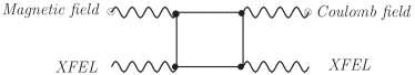
Figure 1: Exemplary Feynman diagram of the considered process (wavy/straight lines represent photons/electrons).

In contrast to the cases mentioned above, the interaction of electromagnetic fields (as predicted by QED) in a regime well below the QED scales $mc^{2}$, $E_{\rm crit}$ and $B_{\rm crit}$ has not been observed yet. Prominent proposals for ongoing and planned experiments include the interaction of an optical (or near-optical) laser with a (quasi) static magnetic field of a few Tesla, see, e.g., della-16 ; pvlas ; zava-12 ; zava-06 ; zava-08 ; OVAL ; BMV ; hartman-17 ; battesti-18 , the interaction of x-ray free electron laser (XFEL) beams among each other or with optical lasers, see, e.g., heinzl-06 ; inada-14 ; yamaji-16 ; Schlenvoigt-2016 ; Karbstein-2016 ; inada-2017 , or the interaction of several optical lasers, see, e.g., dipiazza-07 ; tommasini-09 ; tommasini-10 ; koga-17 ; king-12 ; gies1 ; gies2 ; gies3 ; gies-09 ; grote-15 ; ahm-20 .

Here, we consider a mixed set-up where an XFEL beam is scattered at the combination of a strong magnetic field $\bf{B}_{\rm ext}$ superimposed by the Coulomb field $\bf{E}_{\rm ext}$ of a nucleus (as schematically depicted in Fig. 1), see also dipiazza-08 . This scenario offers several advantages: The nuclear Coulomb field facilitates a significant momentum transfer $\Delta\bf k$ while we still obtain a birefringent signal (where the polarization of the XFEL photons flips). The crux of our proposal and the prime difference to the aforementioned scenarios involving nuclear fields studied previously is that we obtain a very large interaction volume whose length and time scales are set by the momentum transfer $\Delta\bf k$ and thus well above the Compton length $\lambdabar$. Hence, all involved field strengths are sub-critical, i.e., well below (1).

Euler-Heisenberg Lagrangian

Since we are considering slowly varying electric $\mathfrak{E}$ and magnetic $\mathfrak{B}$ fields well below $E_{\rm crit}$ and $B_{\rm crit}$, we may start with the lowest-order Euler-Heisenberg Lagrangian ($\hbar=c=\epsilon_{0}=\mu_{0}=1$)

$$\mathfrak{L}=\frac{1}{2}\left(\mathfrak{E}^{2}-\mathfrak{B}^{2}\right)+\xi\left[\left(\mathfrak{E}^{2}-\mathfrak{B}^{2}\right)^{2}+7\left(\mathfrak{E}\cdot\mathfrak{B}\right)^{2}\right],$$ (2)

with a non-linearity set by the parameter

$$\xi=\frac{q^{4}}{360\pi^{2}m^{4}}=\frac{2\alpha_{\rm QED}^{2}}{45m^{4}}=\frac{\alpha_{\rm QED}}{90\pi E_{\rm crit}^{2}}\,,$$ (3)

where $\alpha_{\rm QED}\approx 1/137$ is the fine-structure constant euler+heisenberg , see also review-karbstein-2020 ; review-king+heinzl-2016 ; review-karbstein-2016 ; review-dipiazza-12 ; review-dunne-12 ; akhm-02 ; Bialynicki-Birula-1970 ; Toll-PhD ; adler70 ; adler71 ; adler96 . This is a great advantage because we do not have to construct the electron propagator whose explicit form is known in special cases only foot1 , e.g., in an electromagnetic plane-wave background which facilitates Volkov solutions volkov ; red-65 , see also milstein-05 ; diphatkei-08 ; dipiazza-12 ; dipiazza-14 .

In the weak-field limit considered here, we neglect quadratic terms $\,{\cal O}(\xi^{2})$. Furthermore, we assume that the magnetic field $\bf{B}_{\rm ext}$ is (approximately) constant. In addition to this magnetic field $\bf{B}_{\rm ext}$ and the static Coulomb field $\bf{E}_{\rm ext}$ of the nucleus, we have the space-time dependent XFEL fields ${\bf E}$ and ${\bf B}$. Inserting this split $\mathfrak{E}={\bf E}_{\rm ext}+{\bf E}$ and $\mathfrak{B}={\bf B}_{\rm ext}+{\bf B}$ into (2), we obtain the effective Lagrangian for the XFEL fields (cf. ahm-20 )

$$\mathfrak{L}_{\rm XFEL} = \frac{1}{2}\left[{\bf E}\cdot(\mathbb{1}+\delta\epsilon)\cdot{\bf E}-{\bf B}\cdot(\mathbb{1}-\delta\mu)\cdot{\bf B}\right]$$ (4)

$$+{\bf E}\cdot\delta\Psi\cdot{\bf B}\,,$$

with the symmetric permittivity/permeability tensors $\delta\epsilon^{ij}=8\xi E_{\rm ext}^{i}E_{\rm ext}^{j}+14\xi B_{\rm ext}^{i}B_{\rm ext}^{j}+4\xi\delta^{ij}({\bf E}_{\rm ext}^{2}-{\bf B}_{\rm ext}^{2})$ and $\delta\mu^{ij}=8\xi B_{\rm ext}^{i}B_{\rm ext}^{j}+14\xi E_{\rm ext}^{i}E_{\rm ext}^{j}-4\xi\delta^{ij}({\bf E}_{\rm ext}^{2}-{\bf B}_{\rm ext}^{2})$ plus the symmetry-breaking contribution

$$\delta\Psi^{ij} = -8\xi E_{\rm ext}^{i}B_{\rm ext}^{j}+14\xi B_{\rm ext}^{i}E_{\rm ext}^{j}$$ (5)

$$+14\xi\delta^{ij}({\bf E}_{\rm ext}\cdot{\bf B}_{\rm ext})\,,$$

which describe the polarizability of the QED vacuum. Note that the latter tensor is not symmetric $\delta\Psi^{ij}\neq\delta\Psi^{ji}$.

The equations of motion stemming from (4) can be cast into the same form as the macroscopic Maxwell equations in a medium $\nabla\cdot{\bf D}=0$, $\nabla\cdot{\bf B}=0$, $\nabla\times{\bf E}=-\partial_{t}{\bf B}$, and $\nabla\times{\bf H}=\partial_{t}{\bf D}$, provided that we introduce the electric ${\bf D}=(\mathbb{1}+\delta\epsilon)\cdot{\bf E}+\delta\Psi\cdot{\bf B}$ and magnetic displacement fields ${\bf H}=(\mathbb{1}-\delta\mu)\cdot{\bf B}-\delta\Psi^{\rm T}\cdot{\bf E}$.

Scattering Theory

Now we may calculate the scattering of the XFEL beam with standard approaches, see, e.g., jackson . Combining the above Maxwell equations to

$$\Box{\bf D}=\nabla\times\left[\nabla\times({\bf D}-{\bf E})\right]+\partial_{t}\left[\nabla\times({\bf H}-{\bf B})\right]={\bf J}^{\rm eff}\,,$$ (6)

where the effective source term ${\bf J}^{\rm eff}$ on the right-hand side is small, allows us to employ the Born approximation. To this end, we split the XFEL field ${\bf D}$ into an ingoing plane wave ${\bf D}^{\rm in}$ plus a small scattering contribution ${\bf D}^{\rm out}$ induced by vacuum polarizability $\delta\epsilon$, $\delta\mu$, and $\delta\Psi$. Assuming a stationary time-dependence $e^{-i\omega t}$ for the XFEL field ($\delta\epsilon$, $\delta\mu$, and $\delta\Psi$ are static), we find

$$\Box{\bf D}_{\omega}^{\rm out} = -\left(\nabla^{2}+\omega^{2}\right){\bf D}_{\omega}^{\rm out}={\bf J}_{\omega}^{\rm eff}$$ (7)

$$= \nabla\times\left[\nabla\times(\delta\epsilon\cdot{\bf E}_{\omega}^{\rm in}+\delta\Psi\cdot{\bf B}_{\omega}^{\rm in})\right]$$

$$+i\omega\nabla\times(\delta\mu\cdot{\bf B}_{\omega}^{\rm in}+\delta\Psi^{\rm T}\cdot{\bf E}_{\omega}^{\rm in})\,,$$

where we may approximate ${\bf E}_{\omega}^{\rm in}\approx{\bf D}_{\omega}^{\rm in}$ and ${\bf B}_{\omega}^{\rm in}\approx{\bf H}_{\omega}^{\rm in}$ on the right-hand side within the Born approximation. As usual, solving this Helmholtz differential equation for ${\bf D}_{\omega}^{\rm out}$ with the standard Greens function and considering the behavior at large spatial distances, we find the differential cross section $d\sigma/d\Omega=|{\mathfrak{A}}|^{2}$ with the scattering amplitude jackson

$${\mathfrak{A}}=\frac{1}{4\pi|{\bf D}_{\omega}^{\rm in}|}\,{\bf e}_{\rm out}\cdot\int d^{3}r\,\exp\{-i{\bf k}_{\rm out}\cdot{\bf r}\}\,{\bf J}_{\omega}^{\rm eff}\,,$$ (8)

where ${\bf k}_{\rm out}$ is the wave-number and ${\bf e}_{\rm out}$ the polarization unit vector of the scattered (outgoing) XFEL radiation.

Field-Assisted Scattering

The effective source term ${\bf J}_{\omega}^{\rm eff}$ contains contributions from $\delta\epsilon$, $\delta\mu$, and $\delta\Psi$ which add up to give the full amplitude

$${\mathfrak{A}} = \frac{\omega^{2}}{4\pi}\int d^{3}r\,\exp\{i\Delta{\bf k}\cdot{\bf r}\}\big{[}{\bf e}_{\rm out}\cdot\delta\epsilon\cdot{\bf e}_{\rm in}$$ (9)

$$+{\bf e}_{\rm out}\cdot\delta\Psi\cdot({\bf n}_{\rm in}\times{\bf e}_{\rm in})+{\bf e}_{\rm in}\cdot\delta\Psi\cdot({\bf n}_{\rm out}\times{\bf e}_{\rm out})$$

$$+({\bf n}_{\rm out}\times{\bf e}_{\rm out})\cdot\delta\mu\cdot({\bf n}_{\rm in}\times{\bf e}_{\rm in})\big{]}\,.$$

Here ${\bf n}_{\rm in}$ and ${\bf n}_{\rm out}$ are the initial and final propagation directions (${\bf k}_{\rm in}=\omega{\bf n}_{\rm in}$ and ${\bf k}_{\rm out}=\omega{\bf n}_{\rm out}$), respectively, while ${\bf e}_{\rm in}$ and ${\bf e}_{\rm out}$ denote their polarizations. As usual in scattering theory, the oscillating phase is governed by the momentum transfer $\Delta{\bf k}={\bf k}_{\rm in}-{\bf k}_{\rm out}$.

In the following, we only consider the terms stemming from the combined impact of the magnetic field ${\bf B}_{\rm ext}$ and the nuclear Coulomb field ${\bf E}_{\rm ext}$. Keeping only those cross terms, just the symmetry-breaking contribution $\delta\Psi$ in (5) survives, i.e., we focus on the second line of Eq. (9).

Since ${\bf B}_{\rm ext}$ is (nearly) constant, the spatial integral yields the Fourier transform of the nuclear Coulomb field ${\bf E}_{\rm ext}({\bf r})={\bf e}_{r}Q/(4\pi{\bf r}^{2})$ with the charge $Q=Zq$

$$\int d^{3}r\,e^{i\Delta{\bf k}\cdot{\bf r}}\,\frac{Q}{4\pi{\bf r}^{2}}\,{\bf e}_{r}=iQ\,\frac{\Delta{\bf k}}{(\Delta{\bf k})^{2}}\,.$$ (10)

An important point here is that the $1/r^{2}$ scaling from the Coulomb field cancels the $r^{2}$ volume factor in the $d^{3}r$ integration. As a consequence, the spatial integration is cut off by the momentum transfer $\Delta{\bf k}$ resulting in a very large interaction volume – which may even span many XFEL wavelengths for small scattering angles $|{\bf n}_{\rm in}-{\bf n}_{\rm out}|\ll 1$, i.e., in forward direction. Of course, at some point the approximation of a constant ${\bf B}_{\rm ext}$ breaks down.

Forward Scattering

The large interaction volume mentioned above goes along with a peak in forward direction, i.e., for small $\Delta{\bf k}$, where the signal is enhanced as $\sim 1/|\Delta{\bf k}|$. Since the pre-factor is quite small, let us focus on this leading-order contribution $\sim 1/|\Delta{\bf k}|$. Thus, we approximate ${\bf n}_{\rm in}\approx{\bf n}_{\rm out}\to{\bf n}$ in order to simplify the expressions. In this limit, the isotropic contribution $14\xi\delta^{ij}({\bf E}_{\rm ext}\cdot{\bf B}_{\rm ext})$ in (5) cancels and we are left with the anisotropic terms. For the birefringent signal, where ${\bf e}_{\rm in}$ and ${\bf e}_{\rm out}$ are (nearly) orthogonal, we may approximate ${\bf e}_{\rm out}\approx\pm{\bf n}\times{\bf e}_{\rm in}$ and ${\bf e}_{\rm in}\approx\mp{\bf n}\times{\bf e}_{\rm out}$ which simplifies the integrand in (9) to $\pm[{\bf e}_{\rm out}\cdot\delta\Psi\cdot{\bf e}_{\rm out}-{\bf e}_{\rm in}\cdot\delta\Psi\cdot{\bf e}_{\rm in}]$. Altogether, we get the birefringent amplitude

$${\mathfrak{A}}_{\delta\Psi}^{\perp} = \pm 6i\xi\,\frac{Q}{(\Delta{\bf k})^{2}}\,\frac{\omega^{2}}{4\pi}\left[({\bf e}_{\rm out}\cdot{\bf B}_{\rm ext})({\bf e}_{\rm out}\cdot\Delta{\bf k})\right.$$ (11)

$$\left.-({\bf e}_{\rm in}\cdot{\bf B}_{\rm ext})({\bf e}_{\rm in}\cdot\Delta{\bf k})\right]\,.$$

Thus, one way to obtain a maximum birefringent signal would be to align the momentum transfer $\Delta{\bf k}$ with ${\bf B}_{\rm ext}$ as well as either ${\bf e}_{\rm in}$ or ${\bf e}_{\rm out}$, for example.

In this case, we find the amplitude (up to a sign)

$${\mathfrak{A}}_{\delta\Psi}^{\perp}=6i\xi B_{\rm ext}\,\frac{Q}{|\Delta{\bf k}|}\,\frac{\omega^{2}}{4\pi}=i\,\frac{\alpha_{\rm QED}^{2}}{15\pi}\,\frac{qB_{\rm ext}}{m^{2}}\,\frac{\omega^{2}}{m^{2}}\,\frac{Z}{|\Delta{\bf k}|}\,.$$ (12)

Apart from a numerical pre-factor, this amplitude scales with the ratios of the optical laser field strength $B_{\rm ext}$ over the critical field strength $B_{\rm crit}\approx 4.4\times 10^{9}~{}\rm T$ and the square of the XFEL frequency $\omega$ in comparison to the electron mass $m$.

Detectability

Since the amplitude (12) for field-assisted scattering is proportional to $B_{\rm ext}$ and $\omega^{2}$, it is desirable to have a strong magnetic field and a large XFEL frequency. Ultra-high field strengths $B_{\rm ext}=10^{6}~{}\rm T$ can be reached in the focus of an ultra-strong optical or near optical laser with an intensity of order $10^{22}~{}\rm W/cm^{2}$ in a colliding-beam set-up. Then, inserting an XFEL frequency of $\omega=24~{}\rm keV$, which is still within the range of the European XFEL xfel-data ; Schlenvoigt-2016 ; xfel-URL , we obtain an amplitude of around ${\mathfrak{A}}_{\delta\Psi}^{\perp}\approx 5\times 10^{-13}Z/|\Delta{\bf k}|$ which yields the birefringent differential cross section in forward direction

$$\frac{d\sigma_{\delta\Psi}^{\perp}}{d\Omega}=\left|{\mathfrak{A}}_{\delta\Psi}^{\perp}\right|^{2}\sim 10^{-25}\,\frac{Z^{2}}{(\Delta{\bf k})^{2}}\,.$$ (13)

For a lower frequency of $\omega=1~{}\rm keV$, the amplitude would be reduced to ${\mathfrak{A}}_{\delta\Psi}^{\perp}\approx 10^{-15}Z/|\Delta{\bf k}|$ corresponding to a cross section of $10^{-30}Z^{2}/(\Delta{\bf k})^{2}$.

The suppression in (13) by more than twenty orders of magnitude is roughly comparable to other proposals for vacuum birefringence experiments, see, e.g., heinzl-06 ; Schlenvoigt-2016 . Yet, this suppression does not imply that the effect is beyond reach. In order to demonstrate that, let us discuss two main enhancement factors. The first enhancement factors is a large number $\,{\cal O}(10^{11})$ of polarized XFEL photons, analogous to other vacuum birefringence proposals, see, e.g., heinzl-06 ; Schlenvoigt-2016 . In addition, a large number $N$ of nuclei represents another enhancement factor of our set-up. Note that the peak $\propto 1/(\Delta{\bf k})^{2}$ in forward direction, after integrating over the solid angle $d\Omega$, does only yield a weak (i.e., logarithmic) enhancement. In addition, as explained after (10), this $1/(\Delta{\bf k})^{2}$ behavior is only valid up to minimum values of $|\Delta{\bf k}|$ set by the size of the laser focus. For even smaller $|\Delta{\bf k}|$, one would have to include the Fourier transform of the dependence of ${\bf B}_{\rm ext}({\bf r})$ or ${\bf B}_{\rm ext}(t,{\bf r})$ as an effective form factor.

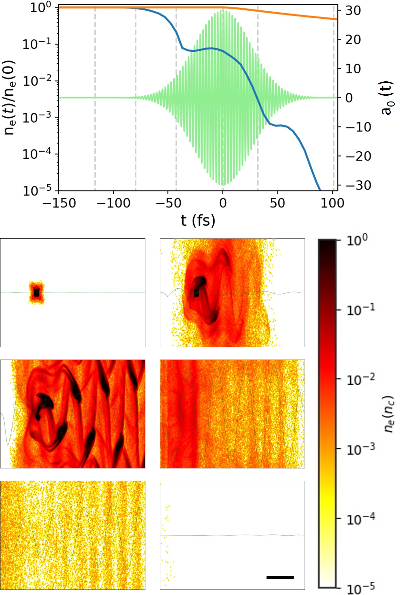
Figure 2: In an exemplary 3D particle-in-cell (PIC) simulation (PIConGPU), a cubic carbon cluster target with 100 nm side length and an (initial) electron density $n_{e}$ of $5\times 10^{23}~{}\rm cm^{-3}$ (i.e., $n_{e}=290~{}n_{c}$) was irradiated by a short pulse laser with 800 nm wavelength, 30 fs width, $1.946\times 10^{21}~{}\rm W/cm^{2}$ intensity (i.e., $a_{0}=30$), incident from the left. In order to assess the number of electrons and ions a transversely oriented XFEL probe beam would observe, we integrated their respective densities perpendicular to the plane shown in the lower panels in a 200 nm $\times$ 200 nm square area. The resulting normalized temporal evolution is plotted in the top: electrons blue, ions orange and the laser electric field is shown in green for reference. The vertical gray dashed lines indicate the times for which the lower panels show the electron density and laser electric field. From top left to bottom right these are $-117$ fs, $-80$ fs, $-43$ fs, $+32$ fs, and $+101$ fs. We see that the electron number in the interaction volume drops by five orders of magnitude while the ion number only decreases moderately (due to the Coulomb explosion). The simulation box has periodic boundaries in the dimensions transverse to the laser; the black scale bar in the bottom right is 500 nm long.

As one possible scenario (see Fig. 2), one may consider a cubic cluster with an edge length of 100 nm with typical solid-state density made of carbon, for example. Then, applying a pre-pulse with a high intensity a bit below $\,{\cal O}(10^{22}~{}\rm W/cm^{2})$, one may blow out almost all electrons, leaving behind $N=\,{\cal O}(10^{8})$ ionized nuclei. Shortly afterwards, before the Coulomb explosion of the remaining nuclei, one would have them interact with the XFEL superimposed by the main pulse (in the form of a colliding beam set-up, for example). To exploit the peak in forward direction, let us assume a small momentum transfer $\Delta\bf{k}$ in the eV regime (corresponding to scattering angles $\vartheta$ of order millirad). In this case, the amplitudes from the $N=\,{\cal O}(10^{8})$ nuclei would have basically the same phase and thus add up coherently, effectively acting as one giant nucleus with charge $Z_{\rm eff}=NZ$. For much larger $\Delta\bf{k}$, one would have to include the spatial distribution of the nuclei in analogy to (10).

For smaller clusters (e.g., 50 nm), the electrons would already be blown out before the laser pulse reaches its peak (see the Appendix). Thus, in this second scenario, one could avoid the “pre-pulse – main pulse” sequence and use the same laser pulse for ionization and assisting Delbrück scattering. However, in this case one should also take into account the electric field component of the optical laser. This electric field of the laser would then generate additional contributions in $\delta\epsilon$ and $\delta\mu$ after combining it with the nuclear Coulomb field. Inserting those additional contributions in $\delta\epsilon$ and $\delta\mu$ into the full amplitude (9), we find that they exactly cancel the terms from $\delta\Psi$ if the optical laser and the XFEL propagate in the same direction. This cancellation does also occur in the case without the nuclear Coulomb field and demonstrates an important difference between a propagating plane wave (crossed fields) and a pure magnetic field. To avoid this cancellation and obtain a birefringent signal, the XFEL should propagate at a finite angle (e.g., perpendicular) to the propagation direction as well as the magnetic field component of the optical laser.

As a third scenario, one could envisage an optical laser focus (expelling the electrons) co-propagating with the XFEL pulse through a less dense medium, in analogy to laser wake-field acceleration Esarey2009 . In the usual set-up, the optical laser would co-propagate with the created fully blown-out plasma cavity and thus also with the XFEL. However, this would again lead to the cancellation problem discussed above. To overcome this problem, one could use an optical laser with a propagation direction different from that of the XFEL, whose focus is co-propagating with the XFEL pulse. This can be achieved by laser pulse-front shaping techniques Debus2019 ; Steiniger2019 ; Steiniger2014 ; Debus2010 . Inserting typical numbers such as a density of order $10^{19}~{}\rm cm^{-3}$, the number $N$ of ions within the interaction region, i.e., the laser focus with a 2.5 $\mu$m spot size, travelling over a distance of order millimeter, would be about two to three orders of magnitude larger $N=\,{\cal O}(6\times 10^{10})$ compared to the first scenario. However, presumably not all of these ions would contribute coherently to the scattering amplitude in view of the larger spatial extent (again compared to the first and second scenario). As an advantage, some of the background processes (see the Appendix) due to the residual electrons and the residual radiation are minimized in the third scenario. In summary, the three scenarios offer different advantages and drawbacks, which should be compared carefully for designing an experimental realization.

Finally, the measurement of the birefringent signal, i.e., the detection of the XFEL photons with flipped polarization could be achieved in complete analogy to other vacuum birefringence proposals, see, e.g., heinzl-06 ; Schlenvoigt-2016 .

Conclusions

As an example for the QED vacuum nonlinearity, we calculate the scattering of XFEL photons at the combined field of a nucleus plus an external magnetic field (e.g., generated by an optical laser focus), see Fig. 1. In contrast to previous work involving nuclear fields, such as pure Delbrück scattering, this scenario yields a large interaction volume, which goes along with a peak of the differential cross section in forward direction $d\sigma/d\Omega\sim 1/(\Delta{\bf k})^{2}$.

As another distinction, the scales relevant to our scenario are well below the characteristic scales of QED mentioned in the Introduction, i.e., the critical field strength (1) and the electron mass $m$. Thus, our scenario is more within the regime where the approximation of a classical electromagnetic field applies – especially for the coherent superposition of the signal from many nuclei – than within the particle (photon) picture often associated with pure Delbrück scattering.

In addition to the normal polarization conserving scattering (see the Appendix), we obtain a birefringent signal (12) whose amplitude ${\mathfrak{A}}_{\delta\Psi}^{\perp}$ is just a little bit smaller. Besides the anisotropy induced by the magnetic field and the aforementioned peak in forward direction, this birefringence may be used to distinguish the process of field-assisted Delbrück scattering considered here from other background processes discussed in the Appendix. Using a large number of XFEL photons xfel-URL ; xfel-data and a large number of nuclei, we show that it might be possible to overcome the suppression of the signal (12) by more than twenty orders of magnitude such that this effect might be observable in the near future at facilities such as the Helmholtz International Beamline for Extreme Fields (HIBEF) at the European XFEL hibef-URL .

I Appendix: Backward Scattering

In contrast to the case of forward scattering discussed above, let us study the opposite case of backward scattering ${\bf n}_{\rm in}=-{\bf n}_{\rm out}$ for comparison. Again focusing on the birefringent signal ${\bf e}_{\rm in}\perp{\bf e}_{\rm out}$, we find

$${\mathfrak{A}}_{\delta\Psi}^{\perp}=i\,\frac{7\alpha_{\rm QED}^{2}}{45\pi}\,\frac{q{\bf B}_{\rm ext}\cdot{\bf n}_{\rm out}}{m^{2}}\,\frac{Z\omega}{m^{2}}\,\,.$$ (14)

In contrast to forward scattering, here the isotropic part $14\xi\delta^{ij}({\bf E}_{\rm ext}\cdot{\bf B}_{\rm ext})$ in (5) contributes while the anisotropic terms cancel. As a consequence, the maximum signal is obtained if the magnetic field ${\bf B}_{\rm ext}$ is aligned with the XFEL propagation direction ${\bf n}_{\rm in}$ and thus perpendicular to both ${\bf e}_{\rm in}$ and ${\bf e}_{\rm out}$.

II Appendix: Parallel Polarizations

To complete our analysis, we also consider the case of parallel polarizations, even though this signal is probably much harder to distinguish from the background processes (see below). Interestingly, for backward scattering ${\bf n}_{\rm in}=-{\bf n}_{\rm out}$, the field-assisted contribution from $\delta\Psi$ vanishes. In forward direction, we get a $1/|\Delta{\bf k}|$ peak in analogy to the birefringent signal (11)

$${\mathfrak{A}}_{\delta\Psi}^{\|} = i\xi\,\frac{Q}{(\Delta{\bf k})^{2}}\,\frac{\omega^{2}}{4\pi}\left[28({\bf e}\cdot{\bf B}_{\rm ext})({\bf n}\times{\bf e})\cdot\Delta{\bf k}\right.$$ (15)

$$\left.-16({\bf e}\cdot\Delta{\bf k})({\bf n}\times{\bf e})\cdot{\bf B}_{\rm ext}\right]\,,$$

where we have set ${\bf e}_{\rm in}$ and ${\bf e}_{\rm out}$ to the overall XFEL polarization unit vector ${\bf e}$. For both polarizations (perpendicular and parallel), the leading-order amplitudes (11) and (15) in forward direction vanish identically if the XFEL propagation direction $\bf n$ is parallel to the magnetic field ${\bf B}_{\rm ext}$. In contrast to the birefringent signal (11), the above amplitude (15) assumes its maximum contribution if the polarization $\bf e$ (i.e., the electric field) of the XFEL is parallel to the magnetic field ${\bf B}_{\rm ext}$ (and thus the XFEL propagation direction $\bf n$ perpendicular to ${\bf B}_{\rm ext}$), while the momentum transfer $\Delta{\bf k}$ is perpendicular to both, i.e., in the “equatorial plane”.

III Appendix: Background Processes

Of course, finding such small differential cross sections (13) necessitates the careful estimate of potential background processes.

III.1 Nuclear Thomson Scattering

Perhaps the most obvious candidate is ordinary Thomson scattering of the XFEL photons by the nuclei themselves. This process is suppressed for heavy nuclei as its amplitude scales inversely proportional to the mass $M$ of the nucleus

$${\mathfrak{A}}_{\rm T}=\alpha_{\rm QED}\,\frac{Z^{2}}{M}\,.$$ (16)

Inserting a typical mass of 0.9 GeV per nucleon, we find that ${\mathfrak{A}}_{\rm T}$ actually becomes comparable to the parallel polarization signal ${\mathfrak{A}}_{\delta\Psi}^{\|}$ in (15) for a momentum transfer in the eV regime. However, Thomson scattering ${\mathfrak{A}}_{\rm T}$ does not display the characteristic (anisotropic) dependence on $\Delta{\bf k}$ and ${\bf B}_{\rm ext}$, for example, and does also not generate a birefringent signal.

III.2 Nuclear Resonances

Similar arguments apply to the scattering of photons by the nuclei via coupling to their internal degrees of freedom, usually referred to as nuclear resonances. Of course, this process does depend on the concrete nuclear structure, such as the nuclear resonance frequencies, which are typically way above the XFEL frequency. As detailed in rev4 , for example, the giant dipole resonance (see, e.g., baldwin-47 ) dominates in such a case – but it is still negligible in comparison to ${\mathfrak{A}}_{\rm T}$ for energies well below the MeV regime. Furthermore, these nuclear resonances do not generate a birefringent signal to lowest order rev4 .

III.3 Delbrück Scattering

Of course, another background process is pure Delbrück scattering, i.e., the interaction of the XFEL beam with the nuclear Coulomb field only. If we estimate the amplitude with the approach described above (in the absence of the optical laser), we find that $\delta\Psi$ vanishes while $\delta\epsilon$ and $\delta\mu$ scale as $1/r^{4}$. Thus, in contrast to ${\mathfrak{A}}_{\delta\Psi}$ considered here, the effective interaction volume would not be large and the spatial integral would be dominated at small (instead if large) radii. Formally, this integral would even diverge for $r\to 0$, but this is an artifact of the used approach based on the leading-order Euler-Heisenberg Lagriangian (2), which is no longer applicable for very small radii since the Coulomb field ${\bf E}_{\rm ext}({\bf r})$ and its gradients become large. Even though it would be a very interesting and non-trivial problem to study Delbrück scattering in this regime, let us obtain a very rough estimate foot2 by cutting off the $r$-integral at the Compton length $\lambdabar$

$${\mathfrak{A}}_{\rm D}\sim Z^{2}\frac{\alpha_{\rm QED}^{3}}{m}\,\frac{\omega^{2}}{m^{2}}\,.$$ (17)

Thus, pure Delbrück scattering is negligible in comparison to the signal ${\mathfrak{A}}_{\delta\Psi}$ considered here.

III.4 Magnetic Field

Going to the other limit, the interaction of the XFEL beam with an optical laser focus only (i.e., without the nucleus) has already been considered in several works, see, e.g., heinzl-06 ; tommasini-09 ; tommasini-10 ; king-12 . Since a constant ${\bf B}_{\rm ext}$ would generate constant $\delta\epsilon$ and $\delta\mu$ such that the spatial integral would yield $\delta^{3}(\Delta{\bf k})$, the possible momentum transfer $\Delta{\bf k}$ is strongly limited by the spatial and temporal inhomogeneities of the optical laser focus, see also dipiazza-08 ; milstein-05 ; dipiazza-07 ; dipiazza-12 ; dipiazza-14 . As another option for discriminating, this process would be independent of the charge $Z$ and the number $N$ of nuclei. Note that the optical laser focus can also generate a birefringent signal.

III.5 Electronic Compton Scattering

Another important background process is Compton scattering from the residual electrons. According to the particle-in-cell (PIC) simulations displayed in Fig. 2, for example, the electron number in the interaction volume drops by a factor of $10^{-5}$ or more, but there may still be a few $\,{\cal O}(10^{4})$ electrons left. Thus, even assuming that the amplitudes from the electrons add up coherently, their lowest-order Thomson scattering signal would already be below the nuclear Thomson scattering ${\mathfrak{A}}_{\rm T}$ as well as the signal ${\mathfrak{A}}_{\delta\Psi}$ considered here. However, this Thomson scattering ${\mathfrak{A}}_{\rm T}=\alpha_{\rm QED}/m$ from the residual electrons does not generate a birefringent signal to lowest order. A birefringent signal can be generated by quantum effects due to the electron spin or by coupling the electrons to the external magnetic field. However, these higher-order processes are suppressed in comparison the the lowest-order Thomson scattering ${\mathfrak{A}}_{\rm T}=\alpha_{\rm QED}/m$.

For example, the birefringent signal from free electrons can be estimated from the Klein-Nishina formula KN1 ; KN2 ; Wig ; Hei

$$\frac{d\sigma_{\rm KN}^{\perp}}{d\Omega}=\frac{\alpha_{\rm QED}^{2}}{m^{2}}\,\frac{\omega^{2}}{m^{2}}\,\frac{\vartheta^{4}}{16}\,,$$ (18)

where $\vartheta\ll 1$ denotes the small scattering angle. The birefringent signal induced by coupling to the external magnetic field can be estimated by the insertion of an additional vertex into the lowest-order Feynman diagram for Compton scattering. The resulting amplitude is suppressed by the inverse combined Keldysh parameter ass1 ; ass2

$$\frac{1}{\gamma}=\frac{qB_{\rm ext}}{m\omega}\,,$$ (19)

which is on the percent level for our parameters. Thus, these effects are sufficiently suppressed in comparison with the signal ${\mathfrak{A}}_{\delta\Psi}^{\perp}$ considered here – unless we have too many residual electrons.

Even for a larger number of residual electrons, one could still observe the desired signal ${\mathfrak{A}}_{\delta\Psi}^{\perp}$ if the unwanted contributions from the electrons would not add up coherently. This would be quite natural since the light electrons are much more prone to de-phasing and decoherence than the heavy nuclei. They experience a stronger recoil and typically have a broader distribution in velocity and position. Further, if the birefringent amplitude depends on the initial electron spin state of the (unpolarized) electrons or if their spin state is changed by the birefringent scattering event, one would get an incoherent superposition.

III.6 Residual Radiation

Further sources for x-ray photons which might lead to a false signal could be radiation processes, such as from the electrons accelerated by the optical laser during ionization or bremsstrahlung effects etc. However, these photons will typically have frequencies different from the XFEL frequency and thus can be filtered out efficiently by the very sharp energy resolution (in the sub-eV regime) of the x-ray polarization filters based on multiple Bragg scattering.

III.7 Interferences

Note that the amplitude ${\mathfrak{A}}_{\delta\Psi}$ derived here is imaginary. This is related to the parity $\mathcal{P}$ symmetry of QED as the Coulomb field ${\bf E}_{\rm ext}({\bf r})$, the symmetry-breaking tensor $\delta\Psi({\bf r})$, and thus also the effective current ${\bf J}_{\omega}^{\rm eff}$ generating ${\mathfrak{A}}_{\delta\Psi}$ are all odd functions of space. In contrast, $\delta\epsilon$ and $\delta\mu$ are even functions, such that the amplitude for pure Delbrück scattering ${\mathfrak{A}}_{\rm D}$ is real – as is the amplitude for Thomson scattering ${\mathfrak{A}}_{\rm T}$. As a result, there are no interference terms (to leading order) between the field-assisted Delbrück scattering ${\mathfrak{A}}_{\delta\Psi}$ considered here and Thomson scattering ${\mathfrak{A}}_{\rm T}$ or Delbrück scattering ${\mathfrak{A}}_{\rm D}$, while there can be interference terms between the latter two ${\mathfrak{A}}_{\rm T}$ and ${\mathfrak{A}}_{\rm D}$.

IV Appendix: PIC simulations

The 3D particle-in-cell simulations shown in Fig. 2 and supplementary Figs. 3 and 4 were performed using the code PIConGPU buss1 ; buss2 , version $0.4.3$ buss3 (Figs. 2 and 3) $0.4.2$ buss4 (Fig. 4). For Figs. 2 and 3, the grid size is $640\times 1280\times 640$, the spatial resolution is $256$ cells per $\lambda_{0}$ ($\lambda_{0}=800$ nm) and the temporal resolution is $6\times 10^{-3}$ fs. For Fig. 4 we employed a moving-window frame with a total size of $256\times 2560\times 1024$ cells which propagates for $50,000$ iterations. The spatial resolution here is $4.5/\lambda_{0}\times 18/\lambda_{0}\times 18/\lambda_{0}$ with a temporal resolution of $103$ as. The electromagnetic field evolution is simulated with the Yee solver yee , while the particle motion is computed using the Boris pusher boris . Particles influence the fields via the Esirkepov current deposition scheme esi with a TSC macro-particle shape hock . Ionization was taken into account for Figs. 2 and 3 by field ionization via the tunneling and barrier suppression del with orbital structure in shielding of the ion charge according to cle1 ; cle2 , as well as by collisions via a modified Thomas-Fermi model more .

IV.1 $50~{}\rm nm$ Carbon Cluster

In analogy to Fig. 2, the PIC simulation for a cubic carbon cluster target at 50 nm side length is shown in Fig. 3. For this smaller cluster, the number of electrons within the interaction volume drops by more than four orders of magnitude before the peak of the laser pulse is reached. In addition, the effect of the Coulomb explosion of the remaining ions is weaker (as expected).

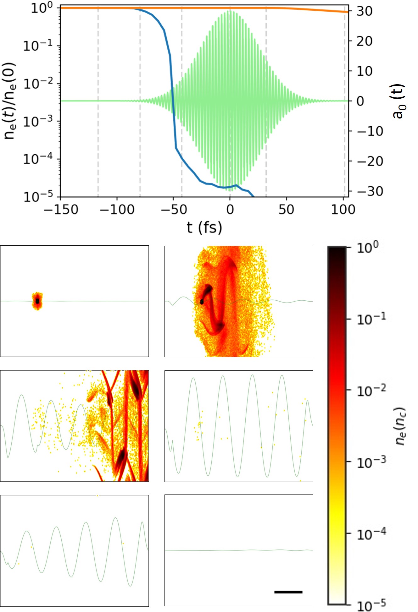
Figure 3: Same as in Fig. 2, but for a cubic carbon cluster target at 50 nm side length.

IV.2 Co-moving Laser Focus

Laser-wakefield acceleration Esarey2009 can sustain a cavity with full electron blowout until reaching laser pump depletion. If an XFEL laser propagates in this blowout in the region for the entire duration where the laser is most intense, electron background is minimal, so that background processes are minimized. For such an approach, lower densities of several $10^{19}~{}\rm cm^{-3}$ are required, because the drive laser pulse dimensions have to be smaller than the plasma wavelength $2\pi c/\omega_{p}$. Compared to high-density targets, see Figs. 2 and 3, this reduction in density is compensated by a much longer interaction length, which can be in the mm-range. However for laser-wakefield acceleration, the drive laser propagation needs to be parallel to XFEL propagation, greatly diminishing the cross-section of laser-assisted Delbrück scattering, so that a different scattering geometry is chosen.

A simplified version of Traveling-wave electron acceleration (TWEAC) Debus2019 , i.e., using one drive laser only, provides a focal region co-moving at the vacuum speed of light with the XFEL laser. Locally in the interaction region of the XFEL laser, the ions see an incoming plane wave coming at some incident angle $\phi$. Globally, the laser is cylindrically focused to a line collinear with the XFEL direction of propagation. Also, in order to maintain a stationary overlap with the XFEL beam, the laser pulse shape has to be prepared to feature a pulse-front tilt of $\phi/2$ Steiniger2019 .

The example shown in Fig. 4 is based on a 3D-PIC simulation, displaying the electron density time-averaged over the full 1 mm interaction length, showing a sizable region devoid of residual electrons (at least 3 orders of magnitudes electron density reduction) in the vicinity of the XFEL pulse and close to maximum laser intensity.

Neither the depletion limit, nor laser pulse guiding constraints limit aforementioned geometry and interaction length, but the laser pulse energy available. For intensities at several $10^{21}~{}\rm W/cm^{2}$ ($a_{0}=30$), laser pulse energies only remain in a technically feasible range if the incidence angle does not become too large and features a tight focus. Furthermore, for minimal differences between initial onset of interaction and the later stationary interaction conditions, it is useful to choose an interaction region close to a steep edge of the gas target. This facilitates full plasma blowout around an XFEL laser over the entire interaction with a gas target.

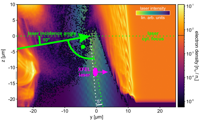
Figure 4: In a 3D-PIC simulation (PIConGPU), an electron blow-out cavity is driven in a 1 mm long $H_{2}$ plasma target at $10^{19}~{}\rm cm^{-3}$ (black-dotted on density scale) using a cylindrically focused, pulse-front tilted laser (800 nm, 30 fs, 335 J, $1.9\times 10^{21}~{}\rm W/cm^{2}$, $a_{0}=30$, 2.5 $\mu$m focus height and 1 mm interaction length) incident at $10^{\circ}$ with respect to the XFEL direction of propagation and $5^{\circ}$ pulse-front tilt. For assessing the amount of residual electrons over the entire interaction length the electron density is time-averaged over the full 1 mm interaction length, showing a sizable region cleared of electrons in the vicinity of the XFEL pulse and close to maximum laser intensity.