From the Fermi blazar sequence to the relation between Fermi blazars and $\gamma$-ray Narrow-line Seyfert 1 Galaxies

Abstract

We use the third catalog of blazars detected by Fermi/LAT (3LAC) and $\gamma$-ray Narrow-line Seyfert 1 Galaxies ($\gamma$-NLSy1s) to study the blazar sequence and relationship between them. Our results are as follows: (i) There is a weak anti-correlation between synchrotron peak frequency and peak luminosity for both Fermi blazars and $\gamma$-NLSy1s, which supports the blazar sequence. However, after Doppler correction, the inverse correlation disappeared, which suggests that anti-correlation between synchrotron peak frequency and peak luminosity is affected by the beaming effect. (ii) There is a significant anti-correlation between jet kinetic power and synchrotron peak frequency for both Fermi blazars and $\gamma$-NLSy1s, which suggests that the $\gamma$-NLSy1s could fit well into the original blazar sequence. (iii) According to previous work, the relationship between synchrotron peak frequency and synchrotron curvature can be explained by statistical or stochastic acceleration mechanisms. There are significant correlations between synchrotron peak frequency and synchrotron curvature for whole sample, Fermi blazars and BL Lacs, respectively. The slopes of the correlation are consistent with statistical acceleration. For FSRQs, LBLs, IBLs, HBLs, and $\gamma$-NLS1s, we also find a significant correlation, but in these cases the slopes can not be explained by previous theoretical models. (iv) The slope of relation between synchrotron peak frequency and synchrotron curvature in $\gamma$-NLS1s is large than that of FSRQs and BL Lacs. This result may imply that the cooling dominates over the acceleration process for FSRQs and BL Lacs, while $\gamma$-NLS1s is the opposite.

1 INTRODUCTION

Blazars are the most extreme active galactic nuclei (AGN) whose jets are pointing towards us. According to the equivalent width (EW) of the optical emission lines, Blazars are usually divided into two subclasses: flat-spectrum radio quasars (FSRQs) and BL Lac objects (BL Lacs). FSRQs have EW $>$5Å, while BL Lacs are smaller than this value (Urry & Padovani, 1995). Later, some authors used other physical parameters to distinguish FSRQs and BL Lacs. Ghisellini et al. (2011) used the ratio of broad emission line luminosity to Eddington luminosity to divide the FSRQs and BL Lacs, namely accretion rate. They pointed out that FSRQs have $\rm{L_{BLR}/L_{Edd}\geq 5\times 10^{-4}}$, while BL Lacs have $\rm{L_{BLR}/L_{Edd}<5\times 10^{-4}}$. This division between FSRQs and BL Lacs may imply that they have different accretion regime (Sbarrato et al., 2014).

Fossati et al. (1998) proposed the so-called “blazar sequence”: the synchrotron peak luminosity and Compton dominance are anti-correlated with the synchrotron peak frequency. By fitting the spectral energy distributions (SEDs) of blazars, Ghisellini et al. (1998) confirmed the discovery of Fossati et al. (1998). They suggested that radiative cooling lead to the formation of a blazar sequence. Some authors supported the blazar sequence (Cavaliere & D’Elia, 2002; Maraschi & Tavecchio, 2003; Maraschi et al., 2008; Ghisellini & Tavecchio, 2008; Chen & Bai, 2011; Finke, 2013; Chen, 2014; Xiong et al., 2015). However, some authors opposed this view (Padovani et al., 2003; Nieppola et al., 2006; Padovani, 2007; Nieppola et al., 2008; Giommi et al., 2012). The authors mainly considered that the selection effect of the samples lead to the blazar sequence. Nieppola et al. (2008) used a low limit Doppler factor to correct for synchrotron peak frequency and peak frequency luminosity. They found that the anti-correlation between synchrotron peak frequency and peak frequency luminosity disappeared. Meyer et al. (2011) used a large sample of radio-loud AGNs to restudy the blazar sequence. They proposed the blazar envelope: Fanaroff–Riley (FR) I radio galaxies and most of BL Lacs are “weak-jet” sources, exhibiting radiatively inefficient accretion. However, low synchrotron-peaking (LSP) blazars and FR II radio galaxies are “strong-jet” sources, exhibiting radiative efficient accretion. Finke (2013) found an anti-correlation exists between Compton dominance and the synchrotron peak frequency by using the Second Large-Area Telescope (2LAT) AGN Catalog (Ackermann et al., 2011). Mao et al. (2016) restudied the blazar sequence by using a large sample of blazars from the Roma-BZCAT catalog. They confirmed the original blazar sequence. Ghisellini et al. (2017) used the third Large-Area Telescope AGN Catalog (Ackermann et al., 2015) to revisit the blazar sequence. They constructed their average spectral energy distribution (SED) by using $\gamma$-ray luminosity, and found that the synchrotron peak frequency is anti-correlated with $\gamma$-ray luminosity. Their results also support the original blazar sequence.

Besides synchrotron peak frequency and synchrontron peak frequency luminosity, the spectral curvature is also an important physical parameter in the SEDs of blazars. The relationship between the synchrotron peak frequency and the spectral curvature can reflect the acceleration process of particles (Massaro et al., 2004, 2006; Paggi et al., 2009; Tramacere et al., 2009, 2011). However, all these previous studies investigated the relationship between SED peak frequency and its curvature by fitting the SEDs through a log-parabolic function, using observational data with spectral windows close to the synchrotron peak frequency. The choice to use broad-band fit of the synchrotron emission, without a proper physical model, can introduce a significant bias in the estimate of the curvature. Chen (2014) predicted the two particle acceleration mechanisms based on the coefficient of relationship between synchrotron peak frequency and spectral curvature. For stochastic acceleration and statistical acceleration, the slope $k$ (1/b_sy = $k$log $\nu_{p}$ + c) is 2, 2.5, and 3.33, respectively. They studied this relation by using 43 blazars and found the slope is 2. This result is consistent with stochastic acceleration.

The $\gamma$-NLSy1s are the mysterious class of the radio-loud AGN. These $\gamma$-NLSy1s show powerful relativistic jets, low black hole mass ($10^{6}-10^{8}M_{\odot}$), and high accretion rate ($0.1-1L_{Edd}$). Some authors thought that their physical properties are similar to blazars. The EW of broad emission line is larger than 5Å for all of $\gamma$-NLSy1s (Oshlack et al., 2001; Zhou et al., 2007; Yao et al., 2015b; Rakshit et al., 2017), which may imply that these $\gamma$-NLSy1s can be formally classified as FSRQs. Foschini (2011) studied the characteristics of the jet of blazars and $\gamma$-NLSy1s. They found that the jet powers of FSRQs and $\gamma$-NLSy1s depend on the black hole mass, while the jet powers of BL Lacs are dependent on the accretion rate. These results suggested that the accretion disk of FSRQs and $\gamma$-NLSy1s are dominated by radiation-pressure, while BL Lacs are dominated by the gas-pressure. Sun et al. (2015) found that the jet properties of $\gamma$-NLSy1s resemble that of FSRQs. Paliya et al. (2018) found that the $\gamma$-NLSy1s and FSRQs occupy the same region in the Wide-field Infrared Survey Explorer (WISE) color–color diagram. What’s more, the $\gamma$-NLSy1s occupy the low black hole mass end of the FSRQs distribution (Paliya et al., 2018). These $\gamma$-NLSy1s may be the counterpart of powerful FSRQs with low black hole mass (Foschini et al., 2015). Chen & Gu (2019) studied the relationship between jet power and accretion disk luminosity in blazars and flat-spectrum radio-loud Narrow-line Seyfert 1 galaxies (FRLNLS1s). They found that the slope of such a relation is similar in FRLNLS1s and blazars. According to the SED modeling, Paliya et al. (2019) found that $\gamma$-NLS1s follow the relation between jet power and accretion luminosity see among blazars. They suggested that the radiation mechanisms of $\gamma$-NLS1s are similar to blazars.

Although many authors have studied the blazar sequence. However, there is no large sample to consider beaming effects when studying the blazar sequence. It has always been controversial about the blazar sequence. At the same time, there is a question: what is the relation between Fermi blazars and $\gamma$-NLS1s? In this paper, we use a large sample of Fermi blazars and $\gamma$-NLSy1s to study blazar sequence and the relation between Fermi blazars and $\gamma$-NLSy1s when considering the beaming effects. The samples are described in Section 2; the results are presented in Section 3; discussions are in Section 4; conclusions are in Section 5. The cosmological parameters $\rm{H_{0}=70kms^{-1}Mpc^{-1}}$, $\rm{\Omega_{m}=0.3}$, and $\rm{\Omega_{\Lambda}=0.7}$ have been adopted in this work.

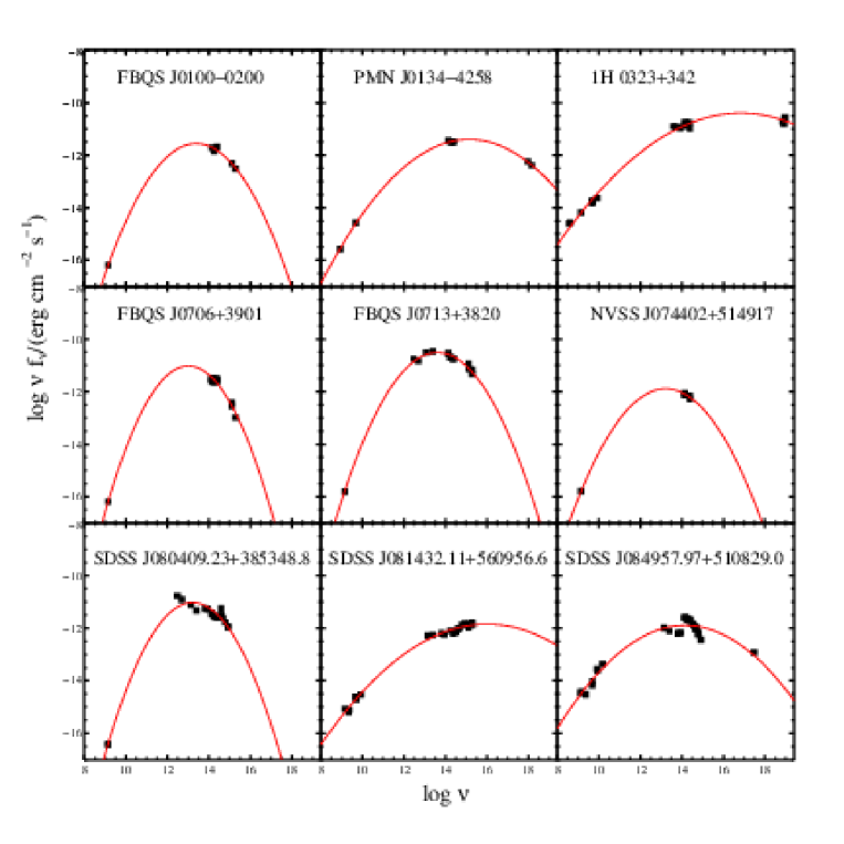
Figure 1: The example of SED fitting of $\gamma$-NLS1s.

2 THE SAMPLE

2.1 The sample of Fermi Blazars

We try to collect a larger sample of Fermi blazars with reliable redshift, synchrotron peak frequency, peak frequency luminosity ($\rm{L_{peak}}$), jet power, and Doppler factor. Firstly, we consider the sample of Fan et al. (2016) to get synchrotron peak frequency and peak frequency luminosity. Fan et al. (2016) compiled the multi-wavelength data of 1425 Fermi blazars from 3FGL (Acero et al., 2015) to calculate their spectral energy distributions (SEDs). They used a parabolic function to fit the multi-wavelength data of 1425 Fermi blazars. The synchrotron peak frequency and peak luminosity were successfully obtained for only 1392 Fermi blazars (461 FSRQs, 620 BL Lacs, and 311 blazars of uncertain type [BCUs]; 999 sources have known redshifts). Secondly, we consider the sample of Chen (2018) to get jet power and Doppler factor. According to the leptonic model, Chen (2018) estimated the jet power and Doppler factor of the 1392 Fermi blazars from the catalog of Fan et al. (2016). Finally, we only use the Fermi blazars with reliable redshift and blazars of certain type. Among the 999 sources with known redshift, 75 were of uncertain type. We therefore get 924 Fermi blazars (461 FSRQ, 463 BL Lacs, see Table 1).

Table 1: The physical parameter of Fermi blazars.

Name	Class	$z$	$\delta$	$\log P_{jet}$	$\log\nu_{peak}$	$\log L_{peak}$	$b$
(1)	(2)	(3)	(4)	(5)	(6)	(7)	(8)
J0001.4+2120	F	1.106	10.7	45.9	16.79	45.70	0.05
J0004.7-4740	F	0.880	12.3	46.2	14.14	46.20	0.12
J0006.4+3825	F	0.229	5.6	45.4	14.03	44.65	0.11
J0008.0+4713	IB	0.280	18.4	46	14.52	44.46	0.12
J0008.6-2340	IB	0.147	51.1	45.8	15.09	44.01	0.10
J0013.9-1853	IB	0.095	29	44.8	14.96	44.37	0.13
J0016.3-0013	F	1.577	6.7	46.4	13.58	45.58	0.09
J0017.6-0512	F	0.227	5	45.1	14.48	44.63	0.11
J0018.4+2947	HB	0.100	14.3	44.9	16.60	43.44	0.06
J0023.5+4454	F	1.062	7.6	46.5	12.78	44.73	0.13
J0024.4+0350	F	0.545	25.5	45.6	13.09	45.37	0.26
J0030.3-4223	F	0.495	6.6	45.8	14.14	45.43	0.12
J0032.3-2852	IB	0.324	71.9	46.5	13.97	44.92	0.15
J0033.6-1921	HB	0.610	12.3	45.1	15.74	45.96	0.11
J0035.2+1513	IB	0.250	27.5	45.5	15.04	44.77	0.12
J0035.9+5949	HB	0.086	14.3	45.6	18.46	44.21	0.04
J0037.9+1239	IB	0.089	25.8	45.6	14.24	43.92	0.14
J0038.0+0012	LB	0.740	14.3	46.4	12.89	45.70	0.25
J0038.0-2501	F	0.498	15.1	45.9	13.26	45.68	0.19

2.2 The $\gamma$-ray narrow-line seyfert 1 galaxies

We try to collect a large sample of $\gamma$-NLS1s with reliable redshift, jet power, and Doppler factor. We consider the sample of Paliya et al. (2019) to get jet power and Doppler factor. Paliya et al. (2019) compiled the largest sample of $\gamma$-NLS1s to study their physical properties. They got the jet power and Doppler factor of 16 $\gamma$-NLS1s based on the leptonic model. Following the work of Fan et al. (2016), we use a parabolic function to fit the quasi-simultaneous multi-wavelength data of 16 $\gamma$-NLS1s and get their synchrotron peak frequency and peak frequency luminosity. The fitting formula is as follows

$$\rm{log(\nu F_{\nu})=-b(log\nu-log\nu_{peak})^{2}+log\nu_{peak}f_{\nu_{p}}},$$ (1)

where $b$ is the spectral curvature, $\rm{log\nu_{peak}}$ is the peak frequency and $\rm{log(\nu_{peak}f_{\nu_{peak}})}$ is the peak flux. The sample of $\gamma$-NLS1s is shown in Table 2. Figure 1 shows the example of SED of $\gamma$-NLS1s.

Table 2: The physical parameter of 16 $\gamma$-NLS1s.

Name	$z$	$\delta$	$\log P_{jet}$	$\log\nu_{peak}$	$\log L_{peak}$	$b$
(1)	(2)	(3)	(4)	(5)	(6)	(7)
1H 0323+342	0.061	13.6	45.82	14.98	45.91	0.99
SBS 0846+513	0.584	19.1	46.05	13.65	45.15	0.88
CGRaBS J0932+5306	0.597	14.7	46.54	15.22	44.93	1.25
GB6 J0937+5008	0.275	15.4	46.41	15.04	44.38	1.14
PMN J0948+0022	0.585	15.7	47.11	15.3	45.00	1.19
TXS 0955+326	0.531	12.3	46.68	14.61	45.79	1.63
FBQS J1102+2239	0.453	19	45.86	13.31	44.98	0.57
CGRaBS J1222+0413	0.966	16.5	47.59	14.95	45.89	1.2
SDSS J124634.65+023809.0	0.362	17.8	45.67	15.67	44.52	1.11
TXS 1419+391	0.49	13.6	46.77	15.15	44.73	1.13
PKS 1502+036	0.407	17.2	46.08	13.34	44.79	0.89
TXS 1518+423	0.484	17.8	46.32	15.9	44.56	1.62
RGB J1644+263	0.145	14.7	45.91	14.56	43.80	0.96
PKS 2004-447	0.24	17.2	45.91	14.67	43.77	1.27
TXS 2116-077	0.26	17.2	45.92	14.46	43.90	1.11
PMN J2118+0013	0.463	14.7	45.99	16.55	44.62	1.35

3 Results

3.1 The correlation between synchrotron peak frequency and peak frequency luminosity

We study the correlation between synchrotron peak frequency and synchrotron peak frequency luminosity using redshift-corrected values. The synchrotron peak frequency luminosity is estimated by using the following formula

$$\rm{L_{peak}=4\pi d_{L}^{2}\nu_{peak}F_{\nu,peak}}$$ (2)

where $d_{L}$ is luminosity distance, $d_{L}(z)=\frac{c}{H_{0}}(1+z)\int_{0}^{z}[\Omega_{\rm{\Lambda}}+\Omega_{\rm{m}}(1+z^{\prime})^{3}]^{-1/2}dz^{\prime}$ (Venters et al., 2009). The redshift-corrected synchrotron peak frequency is calaulated by using formula

$$\rm{\nu_{peak}^{sy}=\nu_{peak}(1+z)}$$ (3)

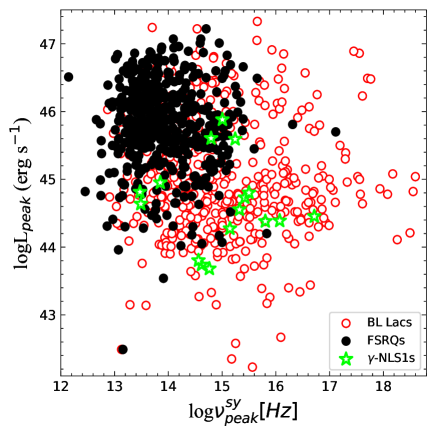
Figure 2: The Synchrotron peak luminosity versus peak frequency for whole sample. The black filled circle is FSRQs.The red empty circle is BL Lacs. The green star is $\gamma$-NLS1s.

Figure 2 shows the relationship between the synchrotron peak frequency luminosity and synchrotron peak frequency. We do not find a “L” or “V” shape in this figure. Fermi blazars and $\gamma$-NLS1s are located in the same region. The $\gamma$-NLS1s tend to have lower synchrotron peak frequency luminosity than FSRQs. The results of Pearson analysis show that there is a weak negative correlation between $L_{peak}$ and $\nu_{peak}^{sy}$ for the whole sample (N = 940, r = -0.25, P = 1.58$\times 10^{-14}$). The scatter of this correlation is $\sigma$= 0.86 dex. The Analysis of Variance (ANOVA) is used to test the results of linear regression, which shows that it is valid for the results of linear regression(value F =60.92, probability P = 1.58$\times 10^{-14}$). At the same time, we also use Kendall and Spearman tests to analyze these correlations besides Pearson. The results of Kendall (r =-0.19, P = 4.81$\times 10^{-19}$) and Spearman (r =-0.29, P = 2.89$\times 10^{-20}$) tests show that there is also a weak anti-correlation between $L_{peak}$ and $\nu_{peak}^{sy}$ for whole sample.

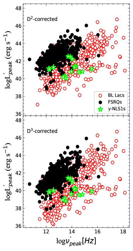
Figure 3: Doppler-corrected synchrotron peak luminosity versus Doppler-corrected synchrotron peak frequency for Fermi blazars. In the top panel, the datapoints are $D^{2}$-corrected. In the bottom panel, the datapoints are D³-corrected.

Nieppola et al. (2008) proposed that the anti-correlation between the synchrotron peak frequency luminosity and synchrotron peak frequency is affected by the beaming effect. Therefore, we use Doppler factor to correct for synchrotron peak frequency and synchrotron peak frequency luminosity. The Doppler-corrected synchrotron peak frequency is performed using equation

$$\nu_{peak}^{{}^{\prime}}=\frac{\nu_{peak}^{sy}}{\delta}$$ (4)

where $\nu_{peak}^{{}^{\prime}}$ indicates the $\delta$-corrected $\nu_{peak}$ in the rest frame. The Doppler-corrected synchrotron peak frequency luminosities are performed using the following formula

$$L_{peak}^{{}^{\prime}}=\frac{L_{peak}}{{\delta}^{P}}$$ (5)

where P= 2+ $\alpha$ is a continuous jet and P= 3+ $\alpha$ is a spherical jet (Urry & Padovani, 1995), spectral index $\alpha$=1.

According to equation (4) and (5), the Doppler-corrected synchrotron peak frequency luminosity and peak frequency can be obtained ($D^{2}$-correction and $D^{3}$-correction indicates P=2+$\alpha$ and P=3+$\alpha$, respectively ). The Doppler-corrected synchrotron peak frequency luminosity versus the Doppler-corrected synchrotron peak frequency is shown in Figure 3. The top panel of Figure 3 (P=2+$\alpha$) shows that there are significant positive correlations for whole sample (r = 0.39, P = 8.77$\times 10^{-35}$). The Analysis of Variance (ANOVA) is used to test the results of linear regression, which shows that it is valid for the results of linear regression(value F = 164.3, probability P = 8.77$\times 10^{-35}$). The results of Kendall (r =0.25, P = 2.42$\times 10^{-30}$) and Spearman (r =0.36, P = 7.20$\times 10^{-30}$) tests show that there is also a correlation between them for whole sample. We can find that there are also significant positive correlations between Doppler-corrected synchrotron peak luminosity and the Doppler-corrected synchrotron peak frequency from the bottom of Figure 3 (P=3+$\alpha$) for whole sample (r = 0.46, P = 1.83$\times 10^{-50}$). The Analysis of Variance (ANOVA) is used to test the results of linear regression, which shows that it is valid for the results of linear regression(value F = 252.1, probability P = 1.83$\times 10^{-50}$). The results of Kendall (r =0.30, P = 4.68$\times 10^{-43}$) and Spearman (r =0.42, P = 5.68$\times 10^{-42}$) tests show that there is also a correlation between them for whole sample.

At the same time, we should also pay attention to the so-called “bulk Lorentz factor crisis” in particular regarding the HBLs and TeV detected HBLs when Doppler correction. The one-zone synchrotron self-Compton process (SSC) model requires much higher Lorentz/Doppler factor values (Tavecchio et al., 1998; Konopelko et al., 2003; Sauge & Henri, 2004; Krawczynski et al., 2001). However, the TeV blazars have no clear superluminal motion, which implies a low Lorentz/Doppler factor in Tev blazars (Piner & Edwarids, 2004; Henri & Sauge, 2006). In our sample, 43 of the 924 sources are Tev blazars. The 43 TeV blazars include 4 FSRQs, 8 intermediate synchrotron peaked BL Lacs (IBLs) and 31 high synchrotron peaked BL Lacs (HBLs). We find that the percentage of TeV blazars is relatively low in our sample, only 4.65%. Therefore, the so-called Lorentz factor crisis does not have a significant impact on our main results when we perform Doppler correction.

3.2 Jet power versus synchrotron peak frequency

The relation between jet kinetic power and the synchrotron peak frequency is shown in Figure 4. From a Pearson analysis, we find that there is a significant anti-correlation between jet kinetic power and the synchrotron peak frequency for the whole sample (r = -0.57, P = 2.75$\times 10^{-81}$). The Analysis of Variance (ANOVA) is used to test the results of linear regression, which shows that it is valid for the results of linear regression(value F = 445.9, probability P = 2.75$\times 10^{-81}$). The results of Kendall (r =-0.38, P = 2.13$\times 10^{-65}$) and Spearman (r =-0.54, P = 1.04$\times 10^{-71}$) tests show that there is also a significant anti-correlation between them for whole sample. What’s more, the $\gamma$-NLS1s follow the blazar sequence.

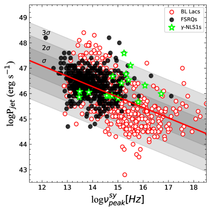
Figure 4: Jet power versus synchrotron peak frequency for whole sample. Shaded areas correspond to 1$\sigma$, 2$\sigma$ and 3$\sigma$ (vertical) dispersion, where $\sigma$ = 0.50 dex. The red line is the least-squares best fit ($\rm{logP_{jet}=-0.41log\nu_{peak}^{{}^{\prime}}+52.03}$). The meanings of the different symbols are the same as in Figure 2.

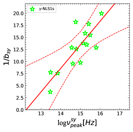
Figure 5: The synchrotron peak frequency versus synchrotron curvature for $\gamma$-NLS1s. The red line is the least-squares best fit ($\rm{1/b_{sy}=(4.87\pm 0.76)log\nu_{peak}^{sy}+(-59.79\pm 11.45)}$). The red dashed line is the 3$\sigma$ confidence level. The meanings of the different symbols are the same as in Figure 2.

3.3 Synchrotron peak frequency versus synchrotron curvature

Figure 5 shows the relationship between the synchrotron peak frequency and synchrotron curvature for $\gamma$-NLS1s. Here we use $1/b_{sy}$ to represent the synchrotron curvature because it will be convenient to compare with the theoretical results (see Chen (2014)). From a Pearson correlation analysis, there is a significant correlation between synchrotron peak frequency and synchrotron curvature for $\gamma$-NLS1s (r = 0.86, p = 1.67$\times 10^{-5}$). The Analysis of Variance (ANOVA) is used to test the results of linear regression, which shows that it is valid for the results of linear regression (value F = 40.88, probability P = 1.67$\times 10^{-5}$). The results of Kendall (r =0.62, P = 0.0007) and Spearman (r =0.78, P = 0.0003 ) tests show that there is also a significant correlation between them for whole sample.

4 Discussions

4.1 The Fermi blazar sequence

In this paper, we use a large sample of Fermi blazars to study the beaming effects on the blazar sequence. Nieppola et al. (2006) and Meyer et al. (2011) found a “V” or “L” shape in the diagrams of $\rm{L_{peak}}$ versus $\rm{\nu_{peak}}$. However, we do not see this shape in Figure 2. Finke (2013) studied blazar sequence by using the 352 second LAT sample. They used the empirical relations of Abdo et al. (2010) to estimate the $\rm{\nu_{peak}}$ and $\rm{L_{peak}}$ and found a significant anti-correlation between the $\rm{\nu_{peak}}$ and $\rm{L_{peak}}$. By comparing Figure 2 with Figure 2 of Finke (2013), we found that Figure 2 is a bit different from the work of Finke (2013). Our results has a larger dispersion than them. These may be due to the different methods. Our sample is larger than that of them. Moreover, we find a weak anti-correlation between synchrotron peak frequency luminosity and the synchrotron peak frequency for the whole sample. These results support the blazar sequence.

The blazar sequence may be affected by the Doppler factor (Nieppola et al., 2008). In the work of Nieppola et al. (2008), the Doppler factor is estimated by using the variability of radio flux, corresponding a lower limit to the Doppler factor. We use the Doppler factor derived from the synchrotron self-Compton (SSC) emission model (Chen, 2018). From Figure 3, we find that after being Doppler-corrected, for all Fermi blazars, the correlations between $\rm{L_{peak}}$ and $\nu_{peak}^{sy}$ become significant positive correlations, i.e. the anti-correlation between $\rm{L_{peak}}$ and $\nu_{peak}^{sy}$ disappears, which is consistent with the result of Nieppola et al. (2008). The observational anti-correlation between $\rm{L_{peak}}$ and $\nu_{peak}^{sy}$ is affected by Doppler beaming factor.

Because synchrotron peak luminosity is strongly affected by the beaming effect. Thus, we study the relationship between intrinsic jet power (jet kinetic power) and the synchrotron peak frequency. We find that there is a significant anti-correlation between $\rm{P_{jet}}$ and $\rm{\nu_{peak}^{sy}}$ for Fermi blazars and $\gamma$-NLS1s, which supports the blazar sequence, i.e. stronger radiative cooling for higher jet power sources results in smaller energies of the electrons emitting at the peaks.

4.2 The relation between Fermi blazars and $\gamma$-NLS1s

Paliya et al. (2013) found that the physical properties of $\gamma$-NLS1s PKS 1502+036 and PKS 2004-447 located between FSRQs and BL Lacs, which imply that theses two sources may belong to the blazar sequence. Foschini (2017) thought that the blazar evolutionary sequence should include NLSy1s. They proposed the evolutionary sequence from NLS1s to BL Lacs, NLS1s$\rightarrow$FSRQs$\rightarrow$BL Lacs, namely from small-mass highly-accretion to large-mass low accreting black hole. We thus study the relation between Fermi blazars and $\gamma$-NLS1s. We fit the SEDs of $\gamma$-NLS1s to get the synchrotron peak frequency and peak frequency luminosity. There is an anti-correlation between the synchrotron peak frequency and peak frequency luminosity for both Fermi blazars and $\gamma$-NLS1s. The $\gamma$-NLS1s follow the synchrotron peak frequency and peak frequency luminosity relation seen among Fermi blazars (Figure 2). At the same time, we also consider the relationship between jet kinetic power and synchrotron peak frequency (Figure 4). There is a significant anti-correlation between jet kinetic power and synchrotron peak frequency for both Fermi blazars and $\gamma$-NLS1s. The $\gamma$-NLS1s follow the jet kinetic power and synchrotron peak frequency relation seen among Fermi blazars. Our results suggest that these $\gamma$-NLS1s could fit well into the traditional blazar sequence. Ghisellini & Tavecchio (2008) proposed that the jet power and the SED of blazars are closely related to the two mian physical parameters of accretion process, namely black hole mass and accretion rate. The radiative cooling leads to the observational phenomenon of blazar sequence (Ghisellini et al., 1998). The FSRQs have high accretion rate, which leads to the fast cooling of relativistic electrons. FSRQs have low synchronous peak frequency and high jet power. However, BL Lacs have low accretion rate, which leads to the slow cooling of relativistic electrons. BL Lacs have high synchronous peak frequency and lower jet power. Some works have found that $\gamma$-NLS1s have high accretion rate (Foschini, 2017; Chen & Gu, 2019). The accretion rate of $\gamma$-NLS1s is similar to FSRQs, which imply that relativistic electrons of the jet of FSRQs and $\gamma$-NLS1s are fast cooling. The $\gamma$-NLS1s may belong to the Fermi blazar sequence.

4.3 Particle acceleration mechanisms for Fermi blazars and $\gamma$-NLS1s

The correlation between log$\nu_{peak}^{sy}$ and $1/b_{sy}$ can be explained by two different scenarios, namely the statistical acceleration and the stochastical acceleration mechanisms (Chen, 2014). Following the same approach of Chen (2014), i.e. to investigate the particle acceleration. We investigate the relationship between log$\nu_{peak}^{sy}$ and $1/b_{sy}$ for Fermi blazars and $\gamma$-NLS1s. The results are shown in Table 3. We get the relationship between log$\nu_{peak}^{sy}$ and $1/b_{sy}$ for whole sample (N = 940, $r$=0.79, F = 1566, $P=3.16\times 10^{-202}$)

$$\rm{1/b_{sy}=(2.44\pm 0.06)log\nu_{peak}^{sy}+(-26.13\pm 0.89)}$$ (6)

and for Fermi blazars (N = 924, $r$=0.79, F =1580, $P=4.27\times 10^{-202}$),

$$\rm{1/b_{sy}=(2.40\pm 0.06)log\nu_{peak}^{sy}+(-25.53\pm 0.88)}$$ (7)

and for FSRQs (N = 461, $r$=0.80, F = 833.5, $P=2.98\times 10^{-105}$),

$$\rm{1/b_{sy}=(3.69\pm 0.13)log\nu_{peak}^{sy}+(-42.89\pm 1.79)}$$ (8)

and for BL Lacs (N = 463, $r$=0.85, F = 1229, $P=3.84\times 10^{-132}$),

$$\rm{1/b_{sy}=(2.56\pm 0.07)log\nu_{peak}^{sy}+(-28.75\pm 1.11)}$$ (9)

and for low synchrotron peaked BL Lacs (LBLs, N = 83, $r$=0.51, F = 28.96, $P=7.02\times 10^{-7}$),

$$\rm{1/b_{sy}=(3.46\pm 0.64)log\nu_{peak}^{sy}+(-40.55\pm 8.73)}$$ (10)

and for intermediate synchrotron peaked BL Lacs (IBLs, N = 214, F = 26.13, $r$=0.33, $P=7.12\times 10^{-7}$),

$$\rm{1/b_{sy}=(1.67\pm 0.33)log\nu_{peak}^{sy}+(-15.72\pm 4.79)}$$ (11)

and for high synchrotron peaked BL Lacs (HBLs, N = 166, $r$=0.80, F = 305.9, $P=2.48\times 10^{-39}$),

$$\rm{1/b_{sy}=(3.09\pm 0.18)log\nu_{peak}^{sy}+(-37.33\pm 2.89)}$$ (12)

and for $\gamma$-NLS1s ($r$=0.86, F = 40.88, $P=1.67\times 10^{-5}$),

$$\rm{1/b_{sy}=(4.87\pm 0.76)log\nu_{peak}^{sy}+(-59.79\pm 11.45)}$$ (13)

Table 3: The Results of Pearson correlation analysis for sample.

sample		$\rm{1/b_{sy}=A\log\nu_{peak}^{sy}+B}$
	A	B	r	p	F
Whole sample	2.44$\pm$0.06	-26.13$\pm$0.89	0.79	$3.16\times 10^{-202}$	1566
Fermi blazars	2.40$\pm$0.06	-25.53$\pm$0.88	0.79	$4.27\times 10^{-202}$	1580
FSRQs	3.69$\pm$0.13	-42.89$\pm$1.79	0.80	$2.98\times 10^{-105}$	833.5
BL Lacs	2.56$\pm$0.07	-28.75$\pm$1.11	0.85	$3.84\times 10^{-132}$	1229
LBLs	3.46$\pm$0.64	-40.55$\pm$8.73	0.51	$7.02\times 10^{-7}$	28.96
IBLs	1.67$\pm$0.33	-15.72$\pm$4.79	0.33	$7.12\times 10^{-7}$	26.13
HBLs	3.09$\pm$0.18	-37.33$\pm$2.89	0.80	$2.48\times 10^{-39}$	305.9
$\gamma$-NLS1s	4.87$\pm$0.76	-59.79$\pm$11.45	0.86	$1.67\times 10^{-5}$	40.88

We find that the slopes of the correlation between synchrotron peak frequency and synchrotron curvature of whole sample ($k_{whole~{}sample}=2.44\pm 0.06$), Fermi blazars ($k_{Fermi~{}blazars}=2.40\pm 0.06$) and BL Lacs ($k_{BLLacs}=2.56\pm 0.07$) are consistent with statistical acceleration for the case of energy-dependent acceleration probability. However, for FSRQs, LBLs, IBLs, HBLs, and $\gamma$-NLS1s, the slopes of the correlation are not consistent with any theoretical values ($k$=5/2, 10/3 and 2).

Chen (2014) used a sample of 43 blazars to study the correlation between synchrotron peak frequency and synchrotron curvature. They got that the slope of the correlation was $2.04\pm 0.03$, which is consistent with the stochastic acceleration. The sample of Chen (2014) was too small to separate them into FSRQs, BL Lacs, LBLs, IBLs, and HBLs. Maybe that’s why they didn’t find different slopes between FSRQs, BL Lacs, LBLs, IBLs, HBLs. At the same time, our results are different from their results, which may be due to the difference in the number of samples.

The slope of the correlation for FSRQs $k_{FSRQs}=3.69\pm 0.13$ is close to 10/3, which can be explained by statistical particle acceleration for the case of fluctuation of the fractional acceleration gain. Xue et al. (2016) studied the relation between synchrotron peak frequency and synchrotron curvature by using a sample of the second LAT AGN catalogue (2LAC). They found that the slope of the correlation for FSRQs is $k_{FSRQs}=3.69\pm 0.24$. Our results are consistent with theirs. We find that the slope of the correlation for IBLs $k_{IBLs}=1.67\pm 0.33$ is close to 2, which can also be explained by stochastic particle acceleration. Kapanadze et al. (2020) studied the X-ray spectral of BL Lacs and found the stochastic acceleration in the relativistic jets of BL Lacs. The slopes of the correlation for LBLs $k_{LBLs}=3.46\pm 0.64$ and HBLs $k_{HBLs}=3.09\pm 0.18$ are close to 10/3, which can be explained by statistical particle acceleration for the case of fluctuations of the fractional acceleration gain.

The slope of the correlation for $\gamma$-NLS1s $k_{\gamma-NLS1s}=4.87\pm 0.76$ is not close to any theoretical values. Its slope is slightly large than that of FSRQs and BL Lacs. These results may be explained in the framework of acceleration and cooling processes (Tramacere et al., 2011). In the acceleration process, there is a significant dispersion on the energy gain, leading to a momentum diffusion term, a decreasing curvature (namely increasing of $1/b_{sy}$) leads to a shift of the peak frequency toward higher peak frequency. Hence, the correlation between the peak frequency and curvature is negative. However, the slope of this correlation can change when the cooling dominates over the acceleration process (Tramacere et al., 2011; Kalita et al., 2019). Tramacere et al. (2011) suggested that the magnetic field plays an important role in the evolution of the spectral parameters. They proposed that when the magnetic field is weak, the evolution of the particles around the peak is dominated by the acceleration process, while it is driven by cooling for strong magnetic field. Paliya et al. (2019) found that the average magnetic field derived for $\gamma$-NLS1s is relatively lower ($\langle B\rangle=0.91\pm 0.33$ G) compared to Fermi blazars (1.83$\pm$0.25 G). These results may imply that the cooling dominates over the acceleration process for Fermi blazars, while the acceleration dominates over the cooling process for $\gamma$-NLS1s. The slopes of $\gamma$-NLS1s, FSRQs and BL Lacs seems to form an evolutionary sequence, $\gamma$-NLS1s$\rightarrow$FSRQs$\rightarrow$BL Lacs, namely from acceleration (high slope) to cooling process (low slope). Foschini (2017) thought that the evolutionary sequence $\gamma$-NLS1s$\rightarrow$FSRQs$\rightarrow$BL Lacs may be the different stages of the cosmological evolution of the same type of source (young$\rightarrow$adult$\rightarrow$old). In the early stage of evolution, the acceleration dominates the spectral evolution. At later stage of evolution, the cooling dominates over the acceleration process (Tramacere et al., 2011). At the same time, we also pay attention to our results might have an intrinsic bias, given by the choice to fit the full low-energy bump of the SED.

5 CONCLUSIONS

We use a large sample of Fermi blazars and $\gamma$-NLS1s to study the Fermi blazar sequence and the relation between them.

1. There is a weak anti-correlation between synchrotron peak frequency luminosity and the synchrotron peak frequency for both Fermi blazars and $\gamma$-NLS1s, which supports the blazar sequence.

2. The Doppler-corrected peak frequency luminosity and Doppler-corrected synchrotron peak frequency is positively correlated for whole sample, which suggests that the relationship between synchrotron peak frequency and synchrotron frequency luminosity is affected by the beaming effect.

3. There is a significant anti-correlation between jet kinetic power and the synchrotron peak frequency for both Fermi blazars and $\gamma$-NLS1s, which suggests that the $\gamma$-NLS1s could fit well into the traditional blazar sequence.

4. There is a significant correlation between synchrotron peak frequency and synchrotron curvature for whole sample, Fermi blazars and BL Lacs, respectively. The slopes of such a correlation are consistent with statistical acceleration for the case of energy-dependent acceleration probability. For FSRQs, LBLs, IBLs, HBLs, and $\gamma$-NLS1s, we also find a significant correlation, but in these cases the slopes can not be explained by previous theoretical models.

5. The slope of relation between synchrotron peak frequency and synchrotron curvature in $\gamma$-NLS1s is large than that of FSRQs and BL Lacs. This result may imply that the cooling dominates over the acceleration process for FSRQs and BL Lacs, while the acceleration dominates over the cooling process for $\gamma$-NLS1s.

References

- Ackermann et al. (2011) Ackermann,M. et al., 2011, ApJ, 743, 171
- Ackermann et al. (2015) Ackermann,M. et al., 2015, ApJ, 810, 14
- Abdo et al. (2010) Abdo, A. A. et al., 2010, ApJ, 716, 30
- Acero et al. (2015) Acero, F., Ackermann, M., Ajello3, M., et al. 2015, ApJS, 218, 23
- Cavaliere & D’Elia (2002) Cavaliere, A.,& D’Elia,V., 2002, ApJ, 571, 226
- Chen & Bai (2011) Chen, L., & Bai, J. M. 2011, ApJ, 735, 108
- Chen (2014) Chen L., 2014, ApJ, 788, 179
- Chen (2018) Chen, L. 2018, ApJS, 235, 39
- Chen & Gu (2019) Chen, Y.Y., & Gu, Q.S. 2019, Ap&SS, 364, 123
- Fan et al. (2016) Fan, J.H., Yang, J.H., Luo, G.Y., Lin, C., Yuan, Y.H., Xiao, H.B., Zhou, A.Y., Hua, X.T., & Pei, Z.Y. 2016, ApJS, 226,20
- Finke (2013) Finke, J.D. 2013, ApJ, 763, 134
- Fossati et al. (1998) Fossati,G., Maraschi,L., Celotti,A., Comastri,A., & Ghisellini,G. 1998, MNRAS,299,433
- Foschini (2011) Foschini,L. 2011, Research in Astron. Astrophys, 11,1266
- Foschini et al. (2015) Foschini, L., Berton, M., Caccianiga, A., et al. 2015, A&A, 575, A13
- Ghisellini et al. (1998) Ghisellini, G., Celotti, A., Fossati, G., Maraschi, L., & Comastri, A. 1998, MNRAS, 301, 451
- Foschini (2017) Foschini, L.2017, Front.Astron. Space Sci. 4, 6
- Ghisellini & Tavecchio (2008) Ghisellini,G., & Tavecchio,F., 2008, MNRAS, 387, 1669
- Ghisellini et al. (2011) Ghisellini G., Tavecchio F., Foschini L, Ghirlanda G., 2011, MNRAS, 414,2674
- Ghisellini et al. (2017) Ghisellini,G., Righi,C., Costamante,L.,& Tavecchio,F. 2017, MNRAS, 469,255
- Giommi et al. (2012) Giommi,P., Padovani,P., Polenta,G., Turriziani,S., D’Elia, V., Piranomonte,S., 2012,MNRAS, 420, 2899
- Henri & Sauge (2006) Henri, G., &Saug, L. 2006, ApJ, 640, 185
- Kapanadze et al. (2020) Kapanadze, Bidzina; Vercellone, Stefano; Romano, P. 2020, New Astronomy, 79
- Kalita et al. (2019) Kalita, N., Sawangwit, U., Gupta, A.C., & Wiita, P.J. 2019, ApJ, 880,19
- Konopelko et al. (2003) Konopelko, A. K., Mastichiadis, A., Kirk, J. G., de Jager, O. C., & Stecker, F. W. 2003, ApJ, 597, 851
- Krawczynski et al. (2001) Krawczynski, H., Coppi, P. S., & Aharonian, F. 2001, ApJ, 559, 187
- Meyer et al. (2011) Meyer, E.T., Fossati, G., Georganopoulos, M., & Lister, M.L. 2011, ApJ, 740, 98
- Maraschi & Tavecchio (2003) Maraschi,L., & Tavecchio,F., 2003, ApJ, 593, 667
- Massaro et al. (2004) Massaro, E., Perri, M., Giommi, P., Nesci,R., 2004a, A&A, 413, 489
- Massaro et al. (2006) Massaro E., Tramacere A., Perri M., Giommi P., Tosti G., 2006, A&A, 448, 861
- Massaro et al. (2014a) Massaro, E., Perri, M., Giommi, P., & Nesci, R. 2004a, A&A, 413, 489
- Massaro et al. (2008) Massaro, F., Tramacere, A., Cavaliere, A., Perri, M., & Giommi, P. 2008, A&A,478, 395
- Maraschi et al. (2008) Maraschi,L., Foschini,L., Ghisellini,G., Tavecchio,F., Sambruna,R.M.,2008,MNRAS, 391, 1981
- Mao et al. (2016) Mao,P., Urry,C.M., Massaro,F., Paggi,A., Cauteruccio,J.,& Künzel,S.R. 2016, ApJS, 224,26
- Nieppola et al. (2006) Nieppola,E., Tornikoski, M., & Valtaoja, E. 2006, A&A, 445, 441
- Nieppola et al. (2008) Nieppola, E., Valtaoja, E., Tornikoski, M., Hovatta, T., & Kotiranta, M. 2008, A&A, 488, 867
- Oshlack et al. (2001) Oshlack, A. Y. K. N., Webster, R. L., Whiting, M. T. 2001, ApJ, 558, 578
- Paliya et al. (2013) Paliya,V.S., Stalin,C.S., Shukla,A., & Sahayanathan,S. 2013, ApJ, 768,52
- Paliya et al. (2018) Paliya,V.S., Ajello,M., Rakshit,S., Mandal,A.K., Stalin,C.S., Kaur,A., & Hartmann,D. 2018, ApJ, 853, L2
- Paliya et al. (2019) Paliya, V.S., Parker, M.L., Jiang, J., Fabian, A.C., Brenneman, L., Ajello, M.,& Hartmann, D. 2019, ApJ, 872, 169
- Padovani et al. (2003) Padovani, P., Perlman,E.S., Landt,H., Giommi,P., Perri,M., 2003,ApJ, 588,128
- Padovani (2007) Padovani,P. 2007, Ap&SS, 309, 63
- Rakshit et al. (2017) Rakshit, S., Stalin, C. S., Chand, H., Zhang, X.G. 2017, ApJS, 229, 39
- Paggi et al. (2009) Paggi, A., Cavaliere, A., Vittorini, V., Tavani, M., 2009, A&A, 508, L31
- Piner & Edwarids (2004) Piner, B.G., & Edwarids, P.G. 2004, ApJ, 600, 115
- Sbarrato et al. (2014) Sbarrato,T., Padovani, & Ghisellini,G. 2014,MNRAS, 445, 81
- Sun et al. (2015) Sun, X.N., Zhang, J., Lin, D.B., Xue, Z.W., Liang, E.W., & Zhang, S.N. 2015, ApJ, 798, 43
- Sauge & Henri (2004) Saug, L., & Henri, G. 2004, ApJ, 616, 136
- Tavecchio et al. (1998) Tavecchio, F., Maraschi, L., & Ghisellini, G. 1998, ApJ, 509, 608
- Tramacere et al. (2007) Tramacere, A., Giommi, P., Massaro, E., et al. 2007, A&A, 467, 501
- Tramacere et al. (2009) Tramacere, A., Giommi, P., Perri, M., Verrecchia, F., & Tosti, G. 2009, A&A,501, 879
- Tramacere et al. (2011) Tramacere, A., Massaro, E., & Taylor, A. M. 2011, ApJ, 739, 66
- Urry & Padovani (1995) Urry, C. M., & Padovani, P., 1995, PASA, 107, 803
- Venters et al. (2009) Venters, T.M., Pavlidou, V., Reyes, L.C. 2009, ApJ, 703, 1939
- Xiong et al. (2015) Xiong,D.R, Zhang, X., Bai,J.M., Zhang,H.J. 2015, MNRAS, 451, 2750
- Xue et al. (2016) Xue, R., Luo, D., Du, L.M., et al. 2016, MNRAS, 463, 3038
- Yao et al. (2015b) Yao, S., Yuan, W., Zhou, H., et al. 2015b, MNRAS, 454,L16
- Zhou et al. (2007) Zhou, H., Wang, T., Yuan, W., et al. 2007, ApJL, 658, L13