The properties and environment of very young galaxies in the local Universe

Abstract

In the local Universe, there is a handful of dwarf compact star-forming galaxies with extremely low oxygen abundances. It has been proposed that they are young, having formed a large fraction of their stellar mass during their last few hundred Myr. However, little is known about the fraction of young stellar populations in more massive galaxies. In a previous article, we analyzed 280 000 SDSS spectra to identify a surprisingly large sample of more massive Very Young Galaxies (VYGs), defined to have formed at least $50\%$ of their stellar mass within the last 1 Gyr. Here, we investigate in detail the properties of a subsample of 207 galaxies that are VYGs according to all three of our spectral models. We compare their properties with those of control sample galaxies (CSGs). We find that VYGs tend to have higher surface brightness and to be more compact, dusty, asymmetric and clumpy than CSGs. Analysis of a subsample with Hi detections reveals that VYGs are more gas-rich than CSGs. VYGs tend to reside more in the inner parts of low-mass groups and are twice as likely to be interacting with a neighbour galaxy than CSGs. On the other hand, VYGs and CSGs have similar gas metallicities and large scale environments (relative to filaments and voids). These results suggest that gas-rich interactions and mergers are the main mechanisms responsible for the recent triggering of star formation in low-redshift VYGs, except for the lowest mass VYGs, where the starbursts may arise from a mixture of mergers and gas infall.

1 Introduction

In the past decades, very deep photometric and spectroscopic surveys have enabled astronomers to trace the cosmic star-formation history (CSFH) from these early epochs to the present (Madau & Dickinson, 2014, and references therein). These observations show that the cosmic star formation rate density peaked approximately $3.5\,$Gyr after the Big Bang ($z\sim 1.9$) and declined exponentially afterwards, with less than $\sim 2\%$ of the stars in the Universe being formed within the last $1\,$Gyr. However, the CSFH is averaged over large volumes and might not represent the star formation histories (SFHs) of individual galaxies. On the contrary, the SFHs of galaxies are observed to vary noticeably with galaxy properties such as mass (Balogh et al., 2009; McGee et al., 2011; Trevisan et al., 2012; Woo et al., 2013), morphology (e.g. Ferrari, de Carvalho & Trevisan, 2015) and with the environment where the galaxies reside (Weinmann et al., 2006; Peng et al., 2010; von der Linden et al., 2010). Among the large variety of assembly histories, the systems that formed more than half of their stellar mass in the last Gyr, which we call hereafter very young galaxies (VYGs), are of particular interest because they offer us a very close view of galaxy formation, allowing us to identify the physical mechanisms that govern the recent growth of stellar mass via gas accretion or gas-rich mergers.

In the local Universe, there are a few low-mass star-forming galaxies that have extremely low oxygen abundances, an indication that they could have formed most of their stars only recently ($<\,1\,$Gyr). A well-studied example is the galaxy I Zw 18, with $12+\log({\rm O/H})\sim 7.2$ (Skillman & Kennicutt, 1993; Izotov & Thuan, 1998), i.e., $\sim 3\%$ of solar metallicity, adopting $12+\log({\rm O/H})=8.7$ for the Sun (Asplund et al. 2009). Using the Hubble Space Telescope (HST) to resolve the stellar content of I Zw 18 and construct colour-magnitude diagrams, Izotov & Thuan (2004) estimated that most of its stellar mass was formed within the last $500\,$Myr. However, deeper HST images revealed the presence of an older stellar component (ages $\mathrel{\hbox{\hbox to0.0pt{\hbox{\lower 4.0pt\hbox{$\sim$}}\hss}\hbox{$>$}}}1-2\,$Gyr, Aloisi et al., 2007; Contreras Ramos et al., 2011). Nevertheless, the fraction of the total stellar mass corresponding to this old population remains undetermined, and if it is less than $50\%$, galaxies such as I Zw 18 could still be classified as VYGs. Other examples of star-forming compact dwarf galaxies that are extremely metal-poor and that have had a considerable fraction of their stellar mass formed during their most recent burst of star formation (SF), a few million years ago, are J0811+4730, the most metal-deficient star-forming galaxy known (Izotov et al., 2018) and J1234+3901 (Izotov, Thuan & Guseva, 2019).

Recent works have suggested that not only dwarf galaxies like I Zw 18, with stellar masses $M_{\star}\sim 10^{7}-10^{8}\,{\rm M}_{\odot}$, but more massive systems can also be very young. Using low resolution ($R\,\sim\,30$) optical spectral energy distributions (SEDs) combined with $ugrizJK$ broad-band photometry, Dressler, Kelson & Abramson (2018) derived the SFHs of galaxies at $0.45<z<0.75$ and identified a population of objects with $M_{\star}>10^{10}\,$${\rm M_{\odot}}$ that formed at least $50\%$ of their stars within the last $\sim 2\,$Gyr of the time of observation. They predicted that these Late Bloomers , account for about $30\%$ of the Milky-Way-sized galaxies ($M_{\star}\sim 10^{10.5}\,$M_⊙) at $z=0.7$, but their frequency declines after $z=0.3$, and they effectively disappear at the present epoch.

Motivated by the debate on the possible VYG nature of very low metallicity galaxies such as I Zw 18, we (Tweed et al., 2018, hereafter Paper I) independently predicted the frequency of VYGs in the local Universe using analytical and semi-analytic models of galaxy formation. We found that the predicted fraction of VYGs depends on galaxy stellar mass, as well as on the model of galaxy formation adopted. The fraction of galaxies with $10^{8}<M_{\star}<10^{10}\,$${\rm M_{\odot}}$ that are VYGs ranges between $\sim 0.4\%$ up to $4\%$ depending on the model, but the fraction of massive galaxies ($M_{\star}\mathrel{\hbox{\hbox to0.0pt{\hbox{\lower 4.0pt\hbox{$\sim$}}\hss}\hbox{$>$}}}10^{11}\,$${\rm M_{\odot}}$) that are VYGs is less than $\sim 0.01\%$ for all models.

In a second article (Mamon et al., 2020, hereafter Paper II), we used the galaxy SFRs inferred from the Sloan Digital Sky Survey - Data Release 12 (SDSS-DR12) spectra to identify the VYGs and computed the fraction of these systems in the local Universe. We found that the observed VYG fractions decreases more gradually with stellar mass when compared to the predictions from Paper I. We also found that the fractions of VYGs strongly depends on the spectral model used in the spectral fitting procedure, with differences up to $1\,$dex between different models, and that the number of VYGs in the SDSS can be as high as a few tens of thousands, depending on the model. Finally, Paper II discusses the possibility that old stellar populations can dominate the mass despite 1) the spectral fitting and 2) the conservative choice of selecting VYGs that have blue colour gradients.

In the present work, we explore in detail the properties of a subsample of the large sample of VYG candidates identified in Paper II, as well as the environment where they reside. To minimize the dependency of SFHs on the spectral model used and select a reliable sample of VYGs, we require that each galaxy in the subsample has more than half of its stellar mass younger than $1\,$Gyr, according to each of three different spectral models.

Our article is organized as follows: in Sect. 2, we describe how we select the VYGs and the control sample galaxies (CSGs). In the following sections, we describe the properties (Sect. 3), gas content (Sect. 4) and environment (Sect. 5) of the VYGs, and compare them with those of the CSGs. In Sect. 6, we summarise how the VYGs differ from other galaxies and discuss our results. Finally, our conclusions are given in Sec. 7. Throughout the paper, we adopt the seven-year Wilkinson Microwave Anisotropy Probe cosmological parameters of a flat Lambda Cold Dark Matter Universe with $\Omega_{\rm m}=0.275$, $\Omega_{\Lambda}=0.725$ and $H_{0}=70.2\,$km$\,{\rm s}^{-1}\,$Mpc^-1 (Komatsu et al., 2011).

2 Data and Sample Selection

2.1 Ages from galaxy spectra

Galaxy SFHs and ages were derived from the SDSS-DR12 spectra using stellar population synthesis analysis. Because they have a fairly high spectral resolution ($R\approx 2000$), a good signal to noise (${\rm S/N}\mathrel{\hbox{\hbox to0.0pt{\hbox{\lower 4.0pt\hbox{$\sim$}}\hss}\hbox{$>$}}}10$), cover a wide spectral range (from below $3800\,$Å to $9200\,$Å) and are flux calibrated, the SDSS spectra allow the derivation of the SFH of each galaxy, by matching the observed spectral energy distribution with a linear combination of single stellar population (SSP) spectra with non-negative coefficients.

As described in Paper II, we considered two non-parametric algorithms to estimate the SFH: the STARLIGHT (Cid Fernandes et al., 2005) algorithm, and the VESPA database (Tojeiro et al., 2009). The two algorithms have been run using the Bruzual & Charlot (2003, hereafter BC03) model, calculated with Padova 1994 stellar evolution tracks (Bressan et al., 1993; Fagotto et al., 1994a, b; Girardi et al., 1996) and assuming the Chabrier (2003) initial mass function (IMF). The BC03 model employs the STELIB stellar library (Le Borgne et al., 2003). VESPA has also been run using the SSPs of Maraston (2005, M05) based on the Kroupa (2001) IMF. We have also run STARLIGHT with the Medium resolution Isaac Newton Telescope Library of Empirical Spectra (MILES, Sánchez-Blázquez et al., 2006), using the updated version 10.0 (Vazdekis et al., 2015, hereafter V15) of the code presented in Vazdekis et al. (2010). The V15 models were computed with the Kroupa (2001) IMF, and stellar evolution tracks from BaSTI (Bag of Stellar Tracks and Isochrones, Pietrinferni et al., 2004, 2006). While STARLIGHT was run assuming a screen dust model and Cardelli, Clayton & Mathis (1989) reddening curve, VESPA assumed either a mixed slab interstellar dust model (Charlot & Fall, 2000) or combined it with extra dust around young stars (also from Charlot & Fall).

We ran STARLIGHT considering 15 bins of ages, ranging from 30 Myr up to 13.5 Gyr, and 6 metallicity bins between [M/H]$\,=-1.3$ and $+0.4$. The SFHs from VESPA were obtained considering 16 bins of ages (from 20 Myr to 14 Gyr) and 4 (for BC03 models) or 5 (for M05 models) bins of metallicity. For each galaxy, and for each one of the models, we compute the median age when the stellar mass was half of its final value by interpolating the cumulative fractional mass as a function of the logarithm of age.

In summary, we have 6 different SFH estimates for each galaxy: those determined with VESPA using BC03 and M05 models, and assuming two different dust modelling in each case; and those obtained with STARLIGHT using BC03 and V15 models. We have investigated how these 6 SFHs correlate with other indicators of recent SF activity, such as the H$\alpha$ equivalent width. We found that, among all models, three (V15 with STARLIGHT, and the 2-component dust BC03 and M05 models with VESPA) lead to a tighter correlation between $f_{\rm young}$ and H$\alpha$ EW (see Paper II for details). Therefore, we have selected these three models as the benchmark for the rest of our analysis. Moreover, because individual SFHs are not fully reliable, we classify a galaxy as a VYG only if all these three models agree on the youth of the galaxy (see Sect. 2.3).

2.2 Handling aperture effects

One of the main issues when dealing with SFHs derived from SDSS spectra is the finite aperture of the SDSS fibres (3 arcsec diameter). These spectra sample only the inner regions of most galaxies. To account for the stars lying outside of the fibre aperture, the stellar masses obtained through the SPS analysis of the SDSS spectra, as described in Sect. 2.1, are corrected by a factor ${\rm dex}[0.4(m_{{\rm fiber},z}-m_{{\rm model},z}]$, where $m_{{\rm fiber},z}$ and $m_{{\rm model},z}$ are the fiber and model magnitudes in the $z$ band. This correction assumes that the SFH is homogeneous throughout the galaxy. We use the $z$-band magnitude because it traces the stellar mass of the galaxy better than bluer filters.

Although the value of the total stellar mass is not strongly affected by assuming the same SFH throughout the galaxy, the finite aperture of the SDSS fibres has a more important consequence on the selection of the VYGs. Many galaxies with blue nuclei have redder envelopes. In fact, 17 per cent of all galaxies in our sample have redder global colours than their fibre colour. Therefore, using spectra within fibres that probe only the nuclei would make us classify mistakenly such galaxies as VYGs, even though the bulk of their stellar mass (in the outer regions) is old.

As discussed in Paper II, this aperture effect is potentially serious, since the median fraction of galaxy light subtended by the fibre, $f_{L}$, is only 26 per cent, and only 3 per cent of our sample have fibres collecting more than half of the galaxy light. Therefore, instead of limiting our sample to galaxies with high $f_{L}$ values, we follow the approach of Paper II and require a VYG galaxy to be one where the $g-i$ colour of the global galaxy (using model magnitudes) is bluer than the corresponding fibre colour.

2.3 Selection of VYG and control samples

2.3.1 Selection of very young galaxies

For our comparison of the properties of VYGs to that of a control sample, we started with the sample of 404 931 SDSS MGS galaxies with $0.005<z<0.12$ that had good spectra and colours (the clean sample described in Sect. 2 of Paper II). We then assembled a sample of VYGs that satisfy the following six additional conditions:

• i) their median ages are younger than 1 Gyr according to all 3 spectral models (V15 with STARLIGHT, and the 2-component dust BC03 and M05 models with VESPA; 1214 galaxies);

• ii) their stellar masses derived with STARLIGHT using V15 models are $\geq 10^{8}\,$M_⊙ (838 galaxies);

• iii) the signal to noise of their SDSS spectra satisfy $\rm S/N\geq 10$, where S/N is computed within a window of $50\,$Å centered at $4755\,$Å (rest frame; 654 galaxies);

• iv) their specific SF rates (sSFRs) are available in the MPA/JHU SpecLineExtra table of the SDSS database (634 galaxies);

• v) they do not lie in the AGN region of the BPT diagram (Baldwin, Phillips & Terlevich, 1981) – we adopted the relation by Kewley et al. (2001) to separate the star-forming and AGN galaxies (633 galaxies);

• vi) they show blue colour gradients: $\Delta(g-i)=(g-i)_{\rm model}-(g-i)_{\rm fiber}\leq 0$ (207 galaxies).

The number of galaxies that remain in the sample after each cut is indicated in parentheses. The list of criteria above is very conservative, and yield a relatively small sample of 207 VYGs. As shown in Paper II, the number of VYGs in the SDSS can be as high as a few tens of thousands, but to avoid possible contaminants in the sample, we opted for the conservative approach. The images of these 207 VYGs are shown in Figs. 24 to 27.

2.3.2 Control sample

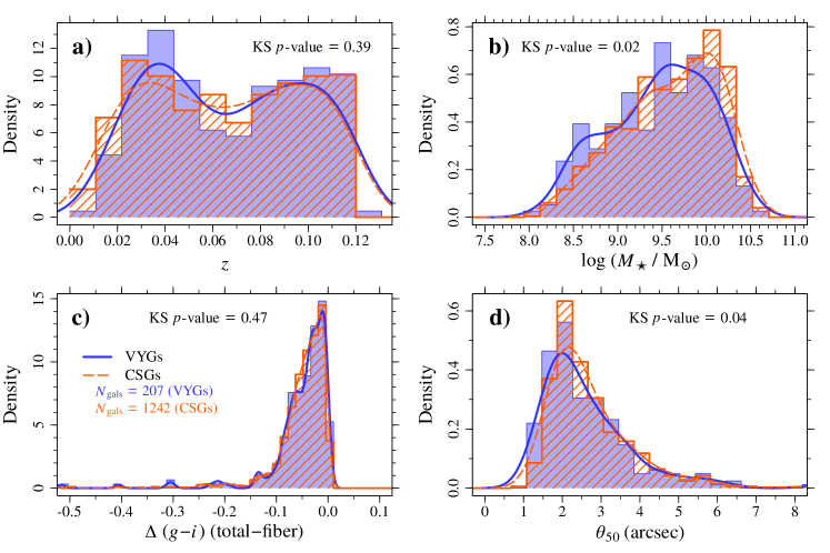
Figure 1: Redshifts (a), stellar masses (b), difference between the total and the fiber $g-i$ colours (c), and angular radius containing 50% of the Petrosian flux, $\theta_{50}$ (d). The blue histograms show the distributions of $z$, $\log\,(M_{\star}/{\rm M_{\odot}})$ (from STARLIGHT V15), $\Delta\,(g-i)$, and $\theta_{50}$ of the VYG sample. The control sample (CSG), drawn from the general sample of galaxies by applying the PSM technique (see the text for details), is shown as the orange histogram. The curves are obtained by smoothing the positions of the data points (not the histograms) using a Gaussian kernel with the standard deviation equal to one third of the standard deviation of the data points. In each panel, we indicate the $p$-value of the Kolmogorov-Smirnov test.

The control sample galaxies (CSGs) were also selected from the clean sample after removing the AGNs using the same criteria adopted for the VYG sample (item v above). The CSGs were chosen to be older than $1\,$Gyr according to all the three models. We matched the CSG galaxies to have the same distributions of redshift, stellar mass (according to STARLIGHT ran with V15), angular size and the total-fibre colour difference, $\Delta(g-i)$ (see item vi above). Matching the radii $\theta_{50}$ containing $50\%$ of the Petrosian flux in the $r-$band ensures that the aperture effects are similar for both samples. The redshifts were included in the matching procedure to ensure that VYGs and CSGs potentially equally populate the same features of the large-scale distribution of galaxies.

We applied the Propensity Score Matching (PSM) technique (Rosenbaum & Rubin, 1983; de Souza et al., 2016) to build the control sample. We used the MatchIt package (Ho et al., 2011), written in R (R Core Team, 2015). This technique allows us to select from the sample of normal galaxies (all minus VYGs) a control sample in which the distribution of observed properties is as close as possible to that of the VYGs. We adopted the Mahalanobis distance approach (Mahalanobis, 1936; Bishop, 2006) and the nearest-neighbour method to perform the matching.

This procedure yielded a sample of 1242 CSGs, i.e. 6 times the size of the VYG sample. We have also tried control samples with different sizes, spanning the range from 1 to 10 times the size of the VYG sample. We found that the results on the comparison between the samples are not affected. The control sample with 6 times the size of the VYG sample was chosen to provide good statistics while keeping the distribution of stellar masses within the same range for both samples.

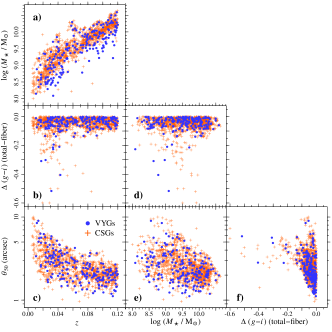
Figure 2: Relations between redshift, stellar mass, difference between the total and the fiber $g-i$ colours, and angular radius containing 50% of the Petrosian flux for the VYGs (blue symbols) and for the CSGs (orange).

The distributions of redshifts, stellar masses, $\Delta(g-i)$, and $\theta_{50}$ of the VYGs and CSGs are shown in Fig. 1. Also shown are the $p$-values derived from the Kolmogorov-Smirnov (KS) test. The VYG and CSG distributions of redshifts, $\Delta(g-i)$ and $\theta_{50}$ (Fig. 1a,c,d) are very similar. On the other hand, we can see in Fig. 1b that the VYG sample contains more low-mass galaxies than the CSG sample. It is particularly difficult to draw a control sample of SDSS galaxies with masses below $\sim 10^{9}\,$M_⊙, since only $\sim 3.5\%$ of them are in this mass range. Besides, $95\%$ of them are at $z\mathrel{\hbox{\hbox to0.0pt{\hbox{\lower 4.0pt\hbox{$\sim$}}\hss}\hbox{$<$}}}0.02$ , the redshift completeness cut-off limit of the SDSS sample defined in Paper II for VYGs within this mass range. This makes it very difficult to select CSGs with the same stellar mass vs. redshift distribution as that of the VYGs. This is illustrated in Fig. 2a, where we see that, at a given mass, the VYGs tend to lie at higher redshifts compared to the CSGs. We have tried to overcome this issue by changing the PSM parameters and the size of the control sample, but we always end up with a similar $M_{\star}$ vs. $z$ distribution. In any event, the results and conclusions presented in this work are not significantly affected by the difference between the VYG and CSG $M_{\star}$ vs. $z$ relations, as we discuss in Sect. 6.7.3. The other panels in Fig. 2 will be discussed in later sections.

3 Properties of very young galaxies

In this Section, we investigate some basic properties of the VYGs by comparing their sSFRs, colours, positions in the BPT diagram (Baldwin et al., 1981), and morphologies with those of the CSGs.

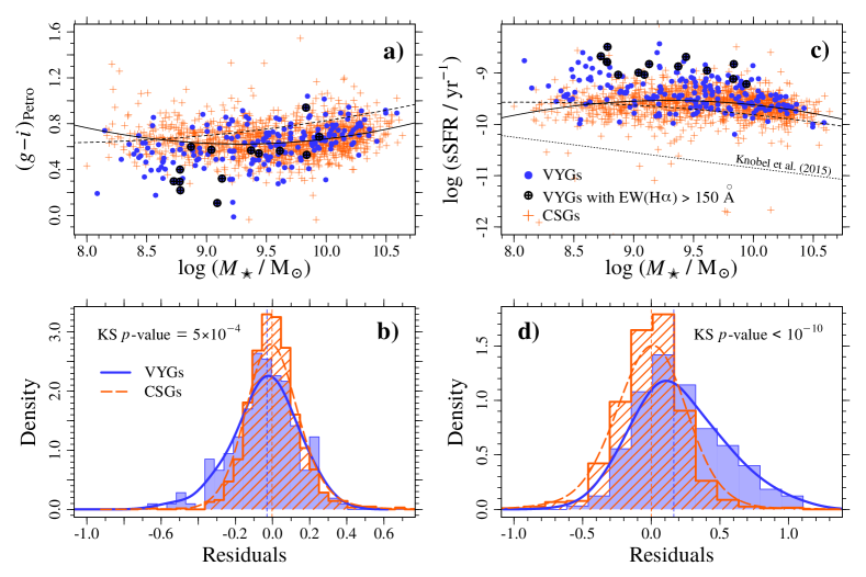
Figure 3: Top: Petrosian $g-i$ colours (a) and specific star formation rates (b, from the MPA/JHU table in SDSS) of VYGs (blue circles) and normal galaxies (orange symbols). The VYGs with EW(H$\alpha$)$\,\geq 150\,$Å are indicated by the black crossed circles. The solid lines in both panels correspond to a second-order polynomial fit to the colour and $\log{\rm sSFR}$ vs. log stellar mass relations for galaxies in the control sample. The dashed lines shows the best-fit relations for a sample of galaxies selected using the same approach adopted to build the control sample, but without including the redshift in the PSM procedure (see text for details). The difference between these two curves illustrates the effect of requiring the CSGs to be at similar distances as the VYGs. The line separating the star-forming and passive galaxies determined by Knobel et al. (2015) is indicated by the dotted line. Bottom: Residuals from the second-order polynomial fits shown for the VYG (blue histograms) and control (orange) samples. In each panel, we indicate the KS test $p$-values.

3.1 Star formation rates and colours

We extracted from the SDSS-DR12 database the optical magnitudes as well as the sSFRs (specsfr_tot_p50 from the galSpecExtra table, obtained with the algorithm of Brinchmann et al., 2004). To compute the $g-i$ colours, we used the extinction- and $k$-corrected Petrosian magnitudes. The $k$-correction was obtained with the kcorrect code (version 4_2) of Blanton et al. (2003), choosing as reference the median redshift of the SDSS sample ($z=0.1$).

In Figure 3, we compare the sSFRs and colours of the VYGs with those of normal galaxies. Although we allow passive galaxies to be included in the control sample, the CSGs are naturally more likely to be star-forming for two reasons. First, $\sim 90\%$ of the galaxies with stellar masses in the range of those of the VYGs are star-forming systems (the line separating the star-forming and passive galaxies determined by Knobel et al., 2015 is shown in Fig. 3c). Second, requiring CSGs to be at similar redshifts and to have similar stellar masses as those of VYGs favours the selection of star-forming systems, since they are brighter and more likely to be seen at distances where VYGs are observed. As described in Sect. 2, the VYG sample contains slightly more low-mass galaxies than the control sample, even after the PSM, since the SDSS-MGS is highly incomplete for stellar masses below $\sim 10^{9}$. To minimize the effects of this difference on our comparison results, we have fitted the relations between the galaxy properties and the stellar mass (using only the galaxies in the control sample) and analysed the residuals from these fits.

The curvature that we observe in the best fits to the $g-i$ and $\log{\rm sSFR}$ vs. stellar mass relations (shown as solid lines in Fig. 3) is, again, a consequence of requiring the CSGs to have a similar redshift distribution as that of the VYGs. If we build a control sample without including the redshift in the PSM procedure, i.e., using only $\log M_{\star}$, $\theta_{50}$, and $\Delta(g-i)$, the $g-i$ colours (sSFRs) of the selected galaxies systematically increase (decrease) with stellar mass, and the best-fit relations (indicated by the dashed curves in Fig. 3) do not show the curvature.

Not surprisingly, the VYGs, which have made more than half of their stellar mass in the last Gyr, show higher sSFRs than the CSGs. The effect is especially evident for the low-mass galaxies ($\log(M_{\star}/{\rm M}_{\odot})<9.0$). The statistical significance of the difference between the 2 samples is $p<10^{-10}$ (Fig. 3a,b). As expected, the VYGs are bluer than normal galaxies, and those with high H$\alpha$ equivalent widths have more extreme sSFRs. Again, the differences are more significant for low-mass galaxies.

The BPT diagram (Baldwin et al., 1981) of the VYG and control samples is shown in Figure 4, where the emission-line fluxes are taken from MPA-JHU catalogue (table galSpecLine based on the SDSS DR12, Brinchmann et al., 2004; Tremonti et al., 2004). We find a higher fraction of VYGs in the composite region of the diagram compared to the normal galaxies (4.5 times higher). By construction of the VYG and CSG samples, there are no galaxies in the AGN region of the diagram. We used the CSGs to derive a fit for the $\log([$O iii$]/{\rm H}\beta)$ vs. $\log([$N ii$]/{\rm H}\alpha)$ relation, and computed the residuals (Fig. 4b). The distribution of the residuals for the VYGs is shifted towards higher ionization levels compared to the CSGs, with a KS test indicating that the difference is statistically significant ($p$-value$\,<10^{-10}$).

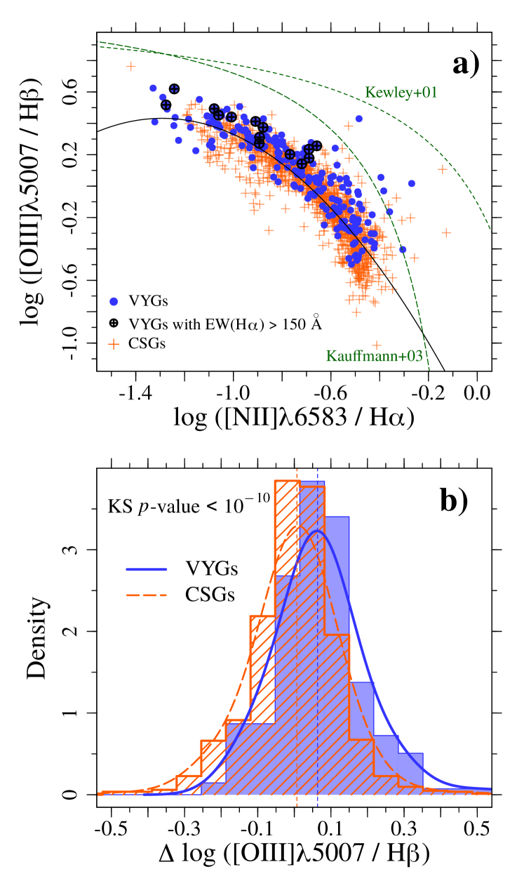
Figure 4: Top: BPT diagram showing the VYG (blue circles) and control (orange symbols) samples. The VYGs with EW(H$\alpha$)$\,\geq 150\,$Å are indicated by the black crossed circles. The relations by Kewley et al. (2001) and Kauffmann et al. (2003) separating star-forming galaxies and AGNs are indicated as short- and long-dashed lines, respectively. The relation between the flux ratios of the CSGs was fitted with a second-order polynomial, as indicated as the black solid line. Bottom: The blue and orange histograms show the distribution of residuals from the polynomial fit for the VYGs and CSGs, respectively.

3.2 Galaxy morphologies and structural parameters

To characterise the VYG and CSG morphologies, we have used the morphological classification from the Galaxy Zoo 1 project (GZ1, Lintott et al., 2011) and that by Domínguez Sánchez et al. (2018, hereafter DS18). The GZ1 catalogue is based on simple visually-inspected classifications by hundreds of thousands of volunteers, and for each galaxy, it provides the debiased fraction of votes for each morphological type and classifies the galaxies in three categories: elliptical, spiral and uncertain. The DS18 catalogue was obtained with Deep Learning algorithms, using Convolutional Neural Networks and visual classification catalogues from Galaxy Zoo 2 project (GZ2, Willett et al., 2013) and by Nair & Abraham (2010) as training sets. Besides providing classifications following a scheme similar to that of the GZ2, it also computes the T-type of each galaxy (de Vaucouleurs, 1963).

We cross-matched our samples with the GZ1 and DS18 catalogues, and found morphological data for nearly all our galaxies: 1384 of our galaxies are in GZ1 (205 VYGs, 1179 CSGs) and 1441 in DS18 (203 VYGs, 1238 CSGs). Most of the VYGs and CSGs are classified as uncertain according to GZ1 (76% and 74%, respectively); all the other VYGs and CSGs are classified as spirals, except for one CSG that is an elliptical. We also compared the distributions of probabilities of being disk- (P_CS_DEBIASED and $p_{\rm disk}$ in the GZ1 and DS18 catalogues, respectively) or bulge-dominated galaxies (P_EL_DEBIASED, $p_{\rm bulge}$), and found no significant difference between the VYGs and CSGs. Finally, the VYG and CSG distributions of T-types from the DS18 catalogue are also very similar. Fig. 5 shows that most of the galaxies ($97.6\%$) have T-type$\geq 0$ (94.1% VYGS, 98.1% CSGs), and a KS test confirms the low statistical differences between the two sample (KS $p$-value$\,=0.54$). We find an excess of VYGs with low T-types compared to the CSGs. The number of VYGs and CSGs that lie below 3$\,\sigma$ of the T-type vs. stellar mass relation is 15 (7.4%) and 27 (2.2%), respectively.

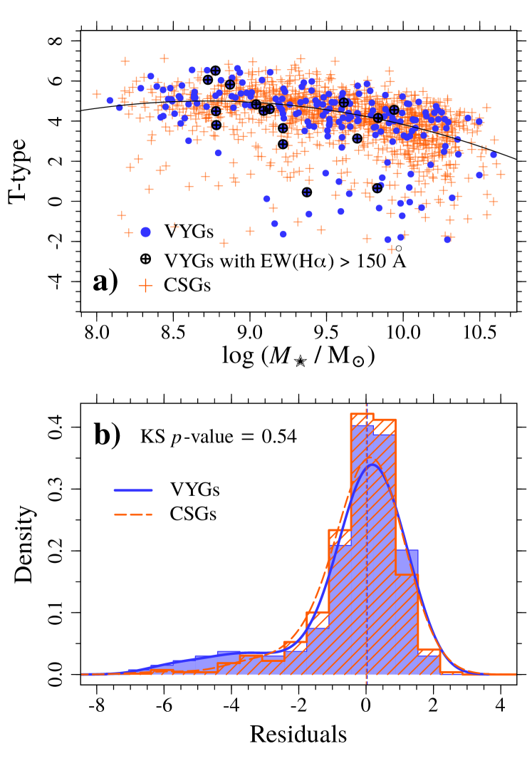
Figure 5: Top: Morphological T-types from Domínguez Sánchez et al. (2018) as a function of stellar mass. The best second-order polynomial fit to the CSG T-type vs. $\log(M_{\star}/{\rm M}_{\odot})$ relation is indicated by the black solid line. Bottom: Distribution of VYG and CSG residuals from the second-order polynomial fit. The notations in both panels are the same as in Fig. 3.

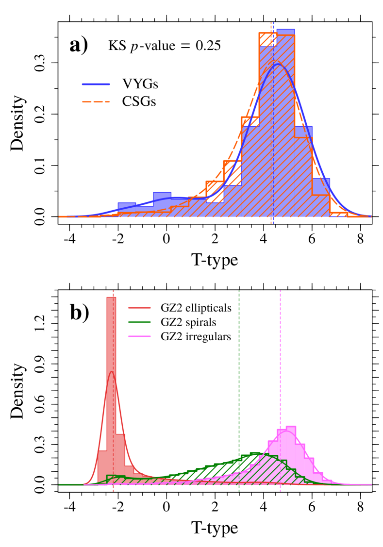
Figure 6: Top: Distributions of T-types of the VYGs (blue histogram) and CSGs (orange). Bottom: Distribution of T-types of galaxies classified as ellipticals (red), spirals (green) and irregulars (magenta) in Galaxy Zoo 2 (GZ2).

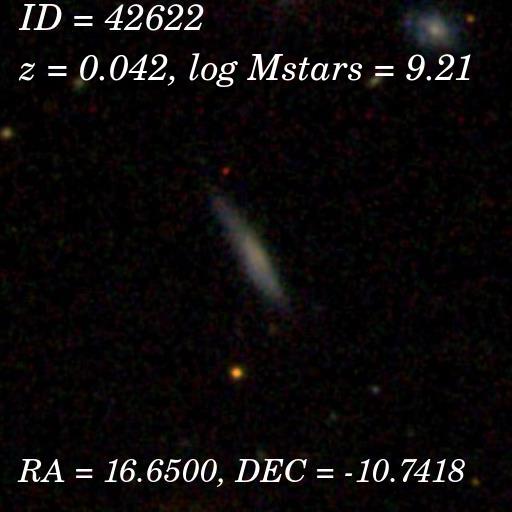
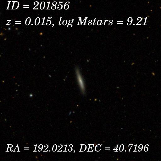
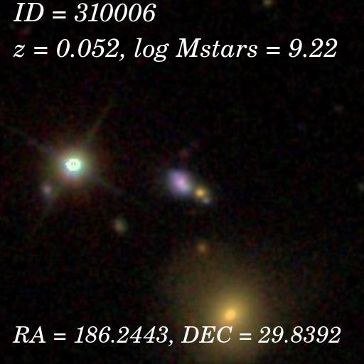
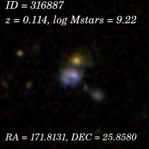
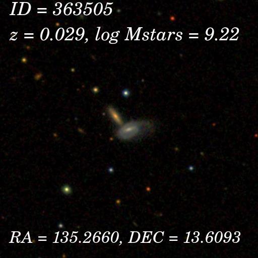
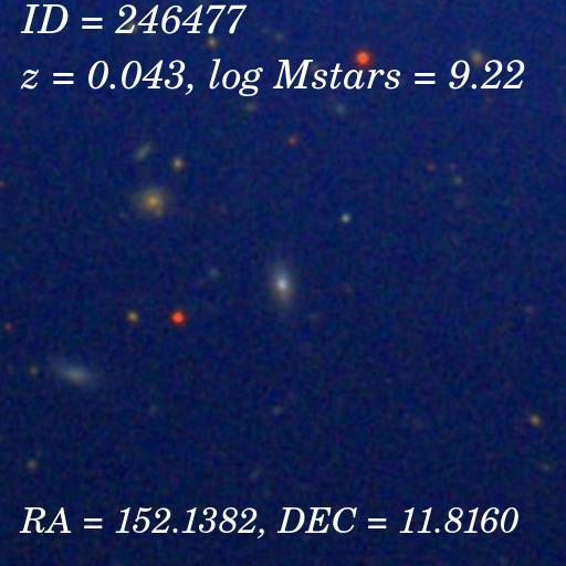
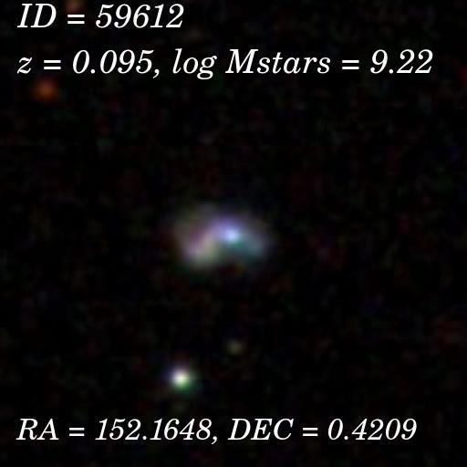
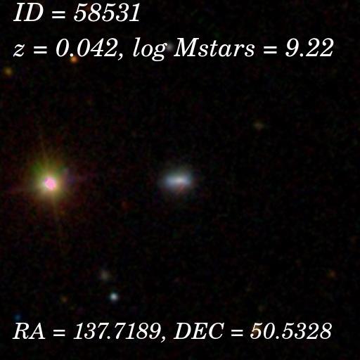
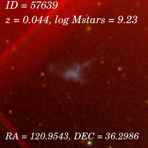
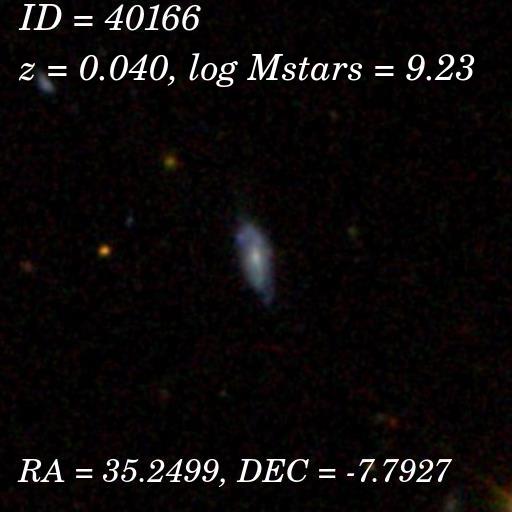
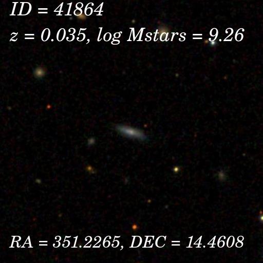
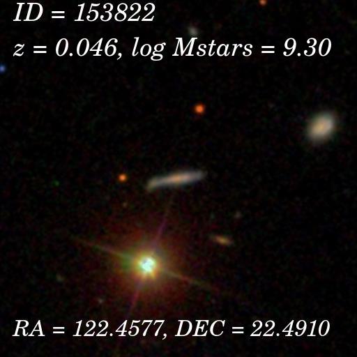
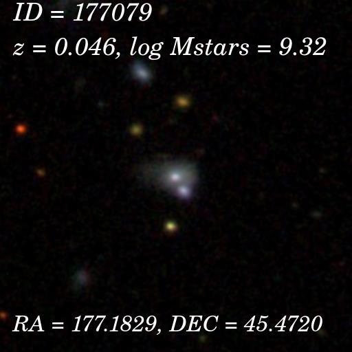
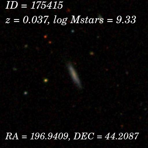
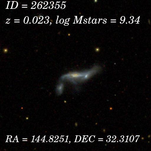
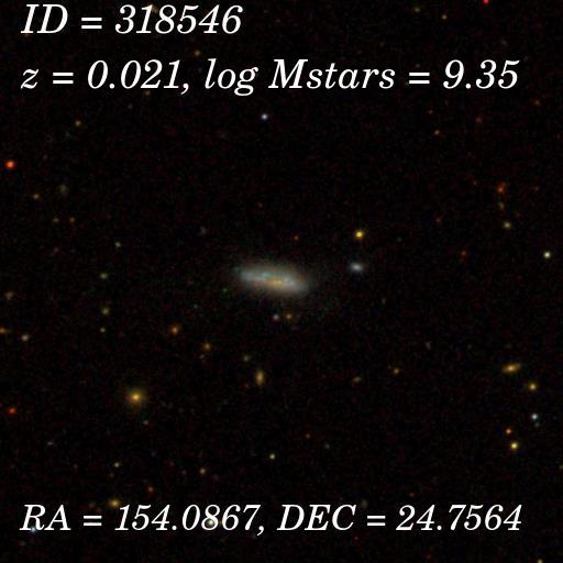
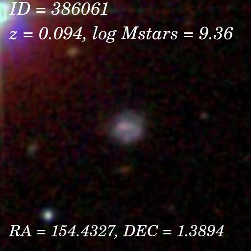
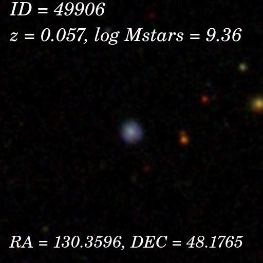
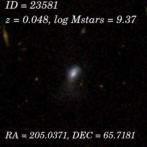
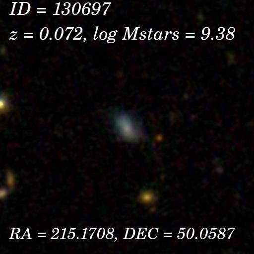
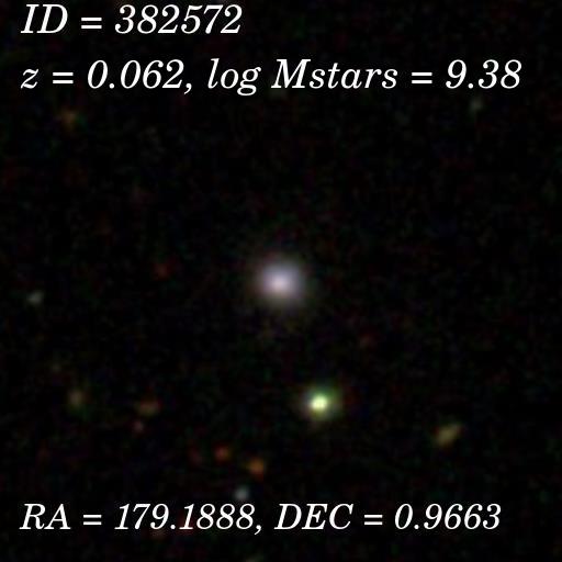
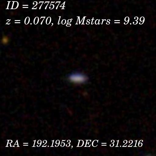
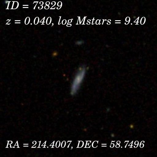
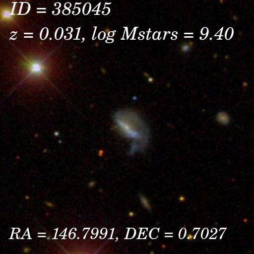
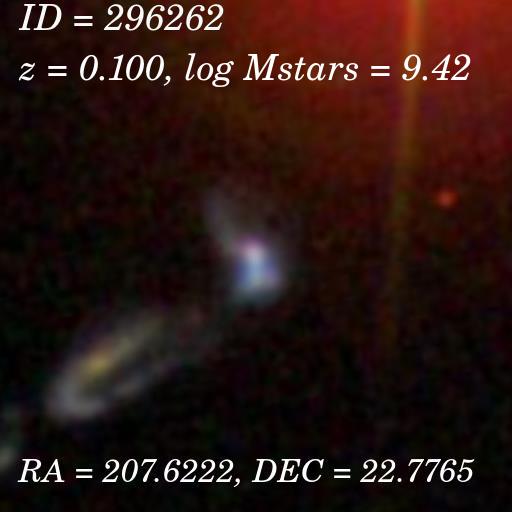
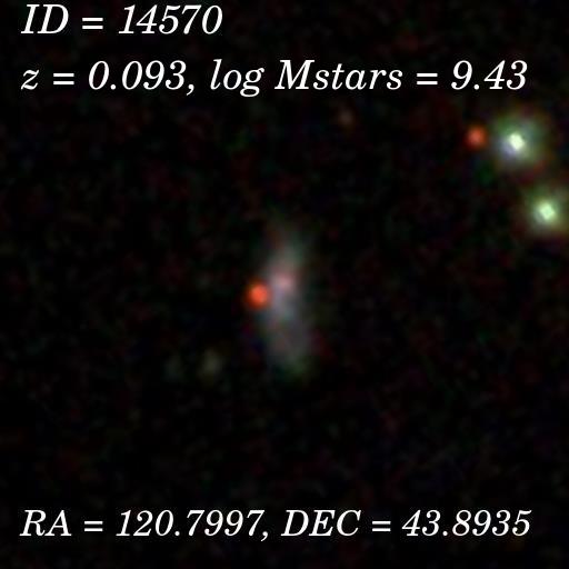
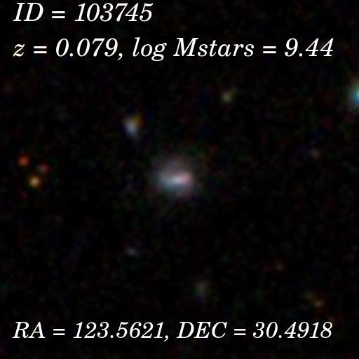
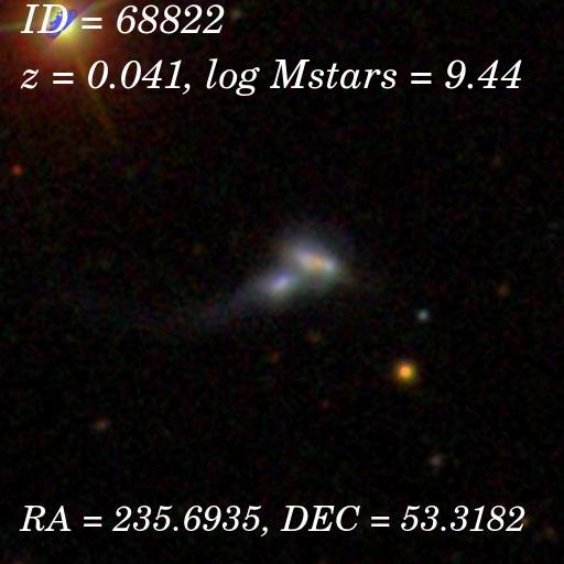
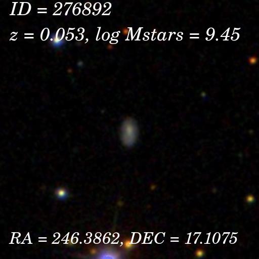
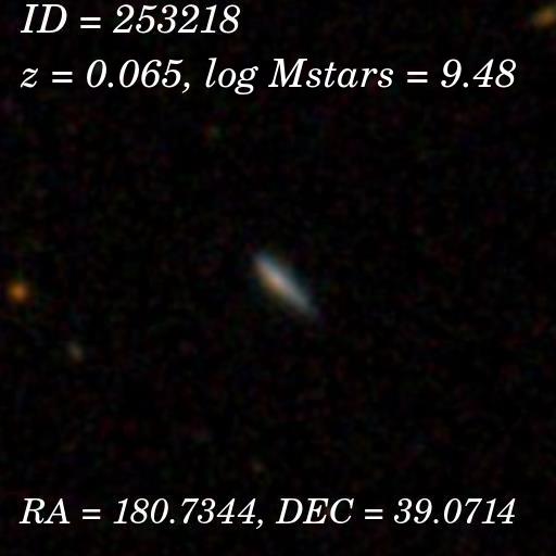
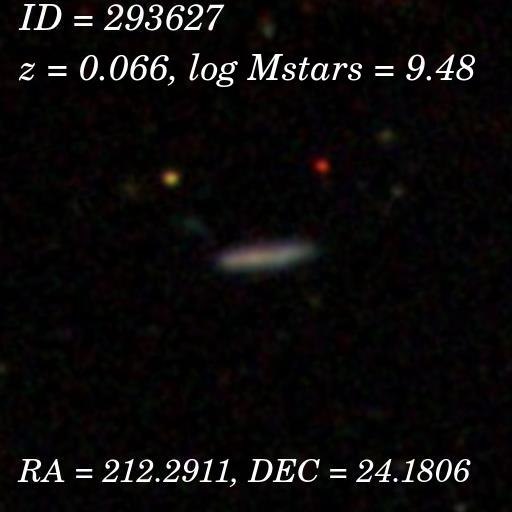
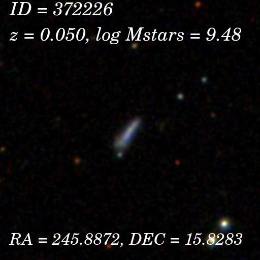
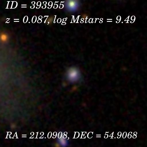
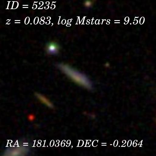
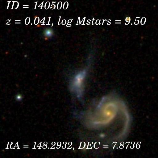
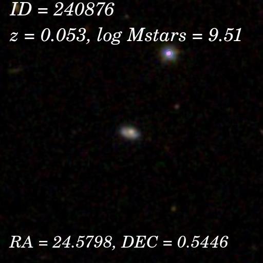
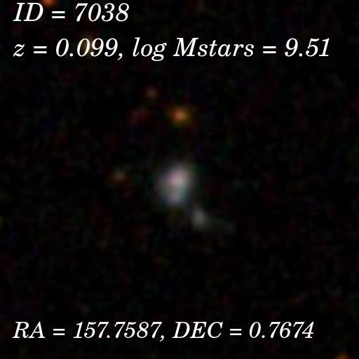
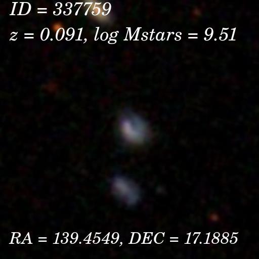
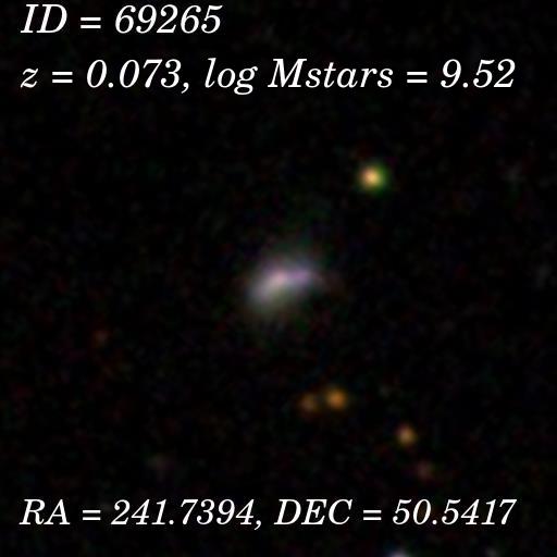
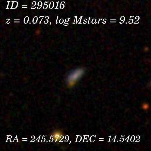
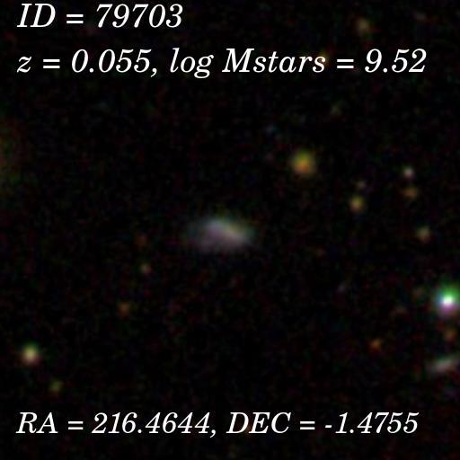
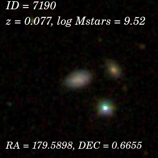
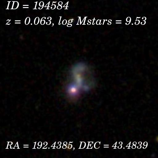
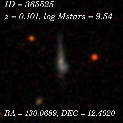
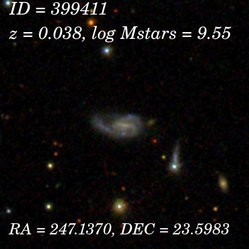
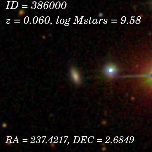
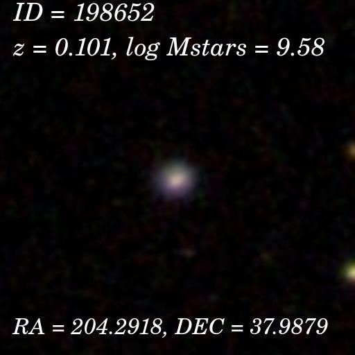
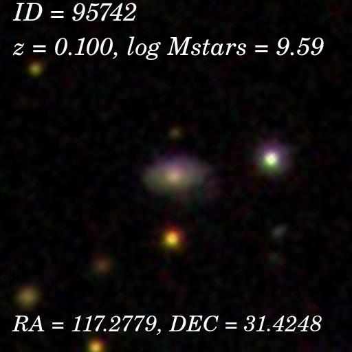
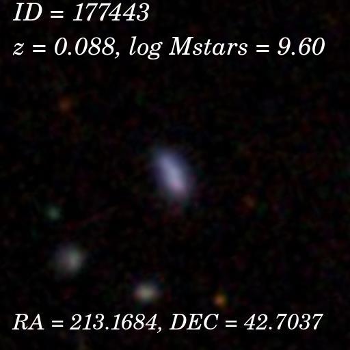
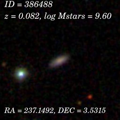
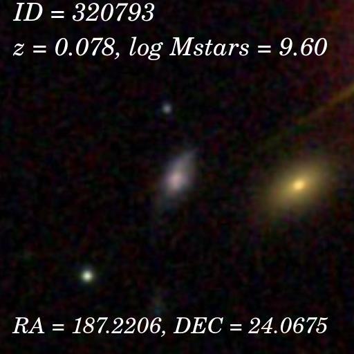
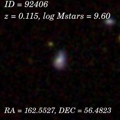
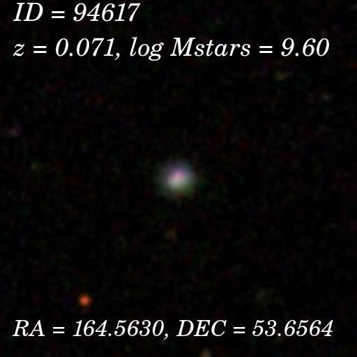
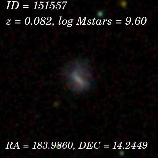
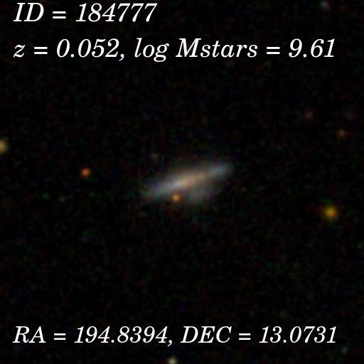
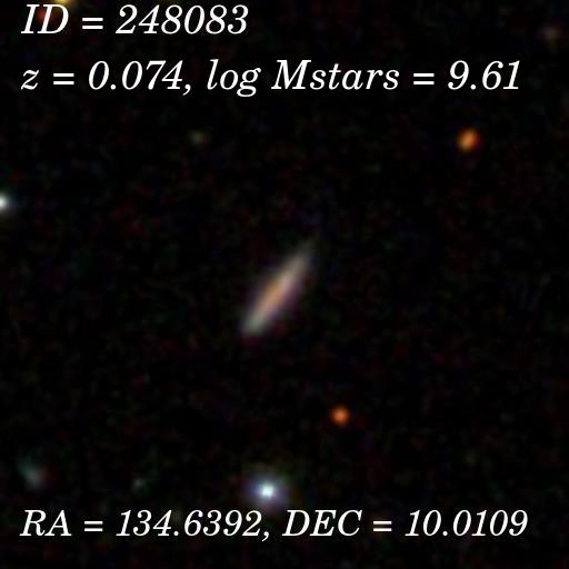
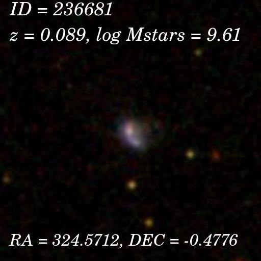
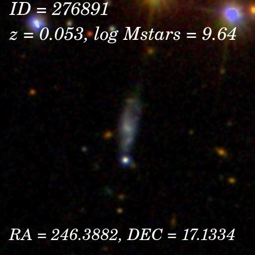
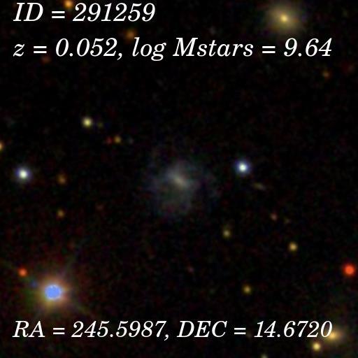
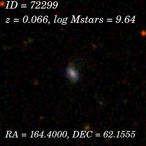
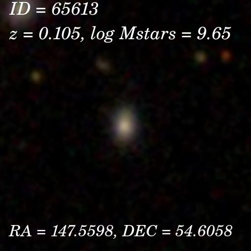
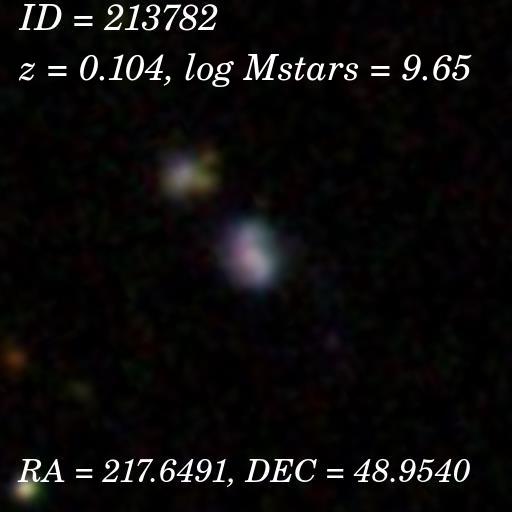
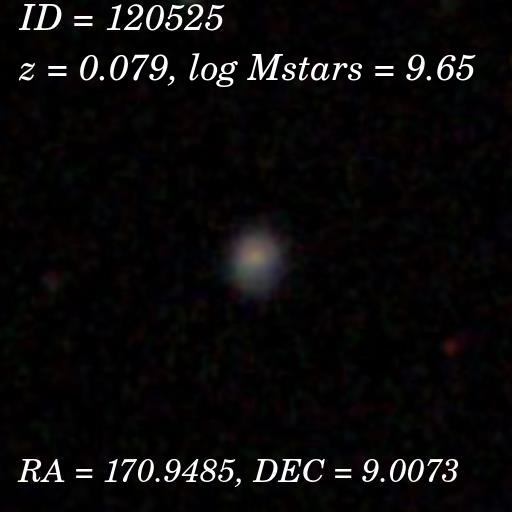
Figure 25: SDSS images of a sample of 207 VYGs. All images are 100 x 100 kpc (cont.).

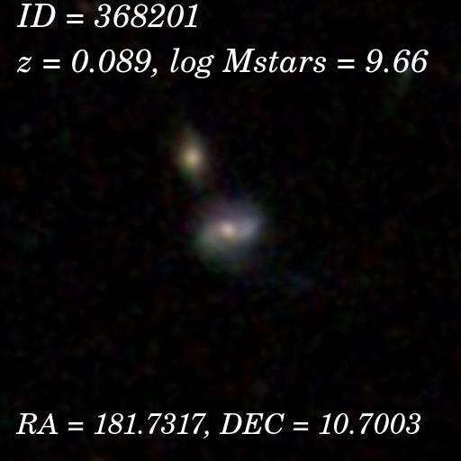
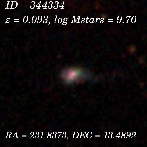
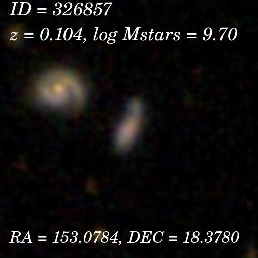
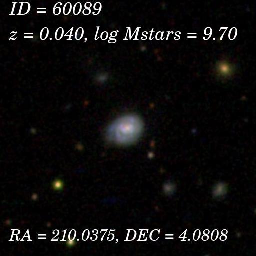
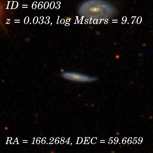
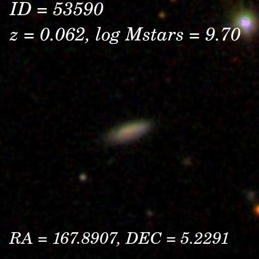
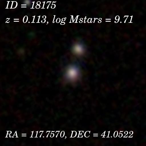
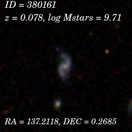
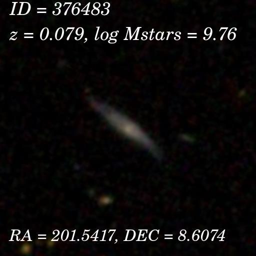
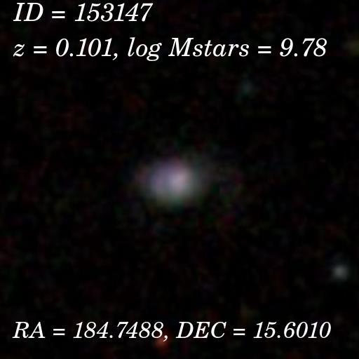
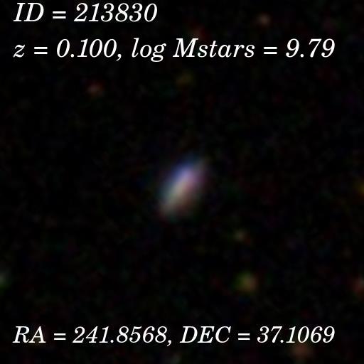
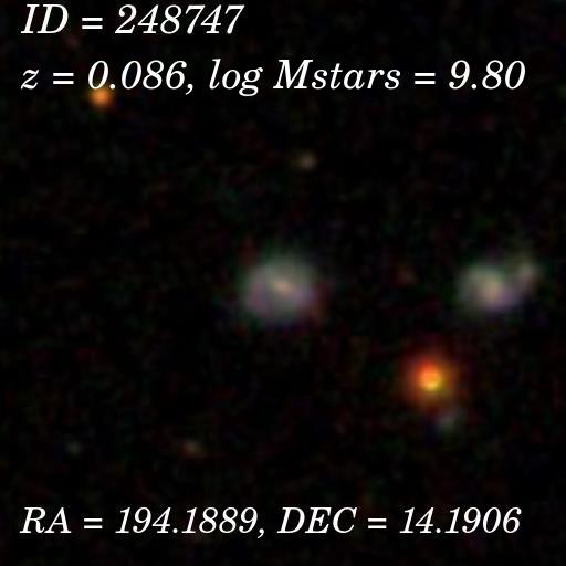
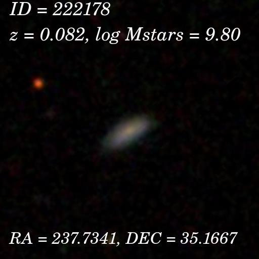
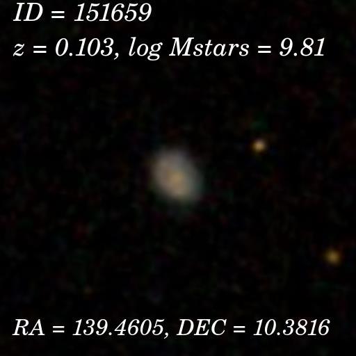
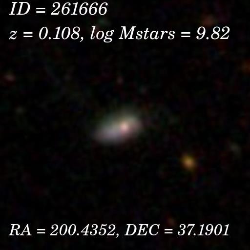
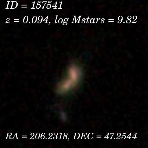
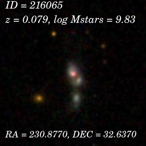
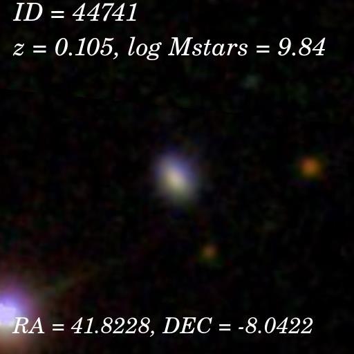
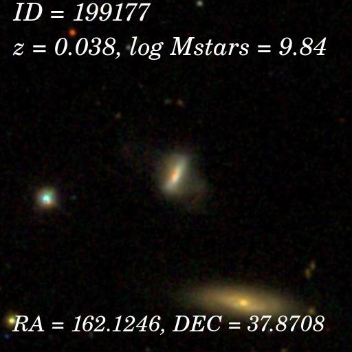
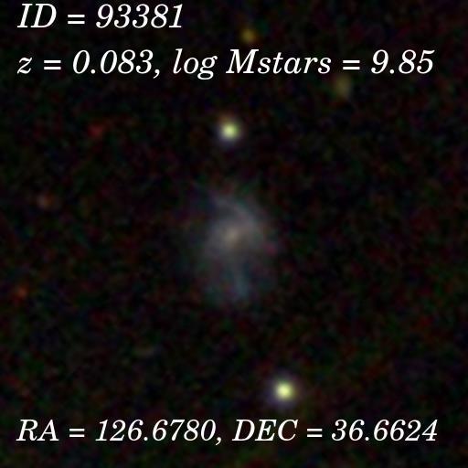
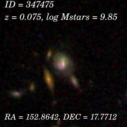
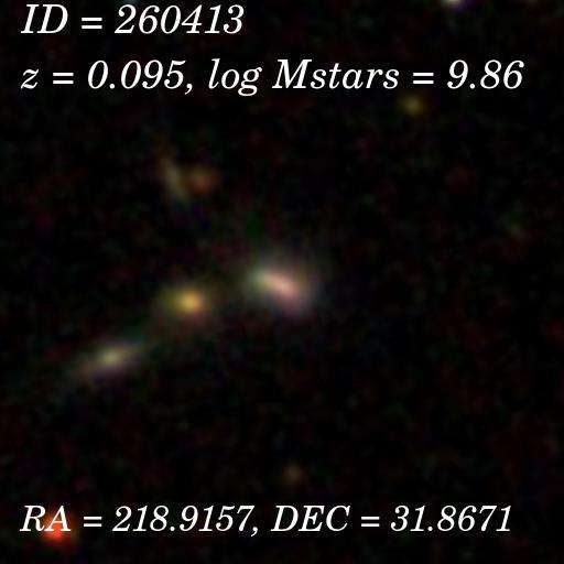
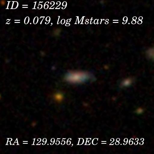
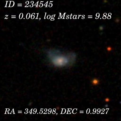
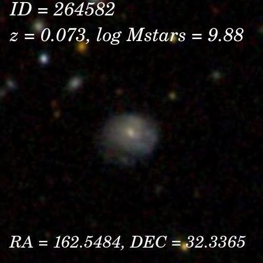
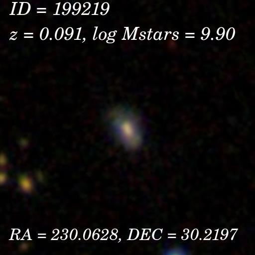
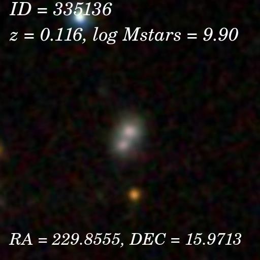
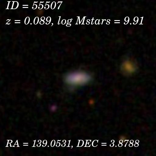
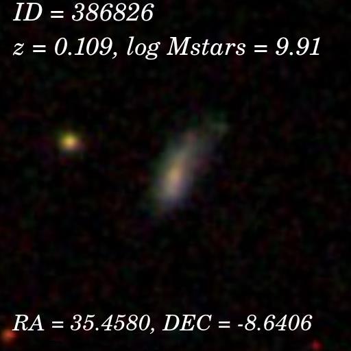
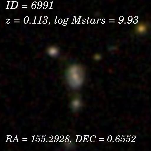
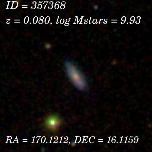
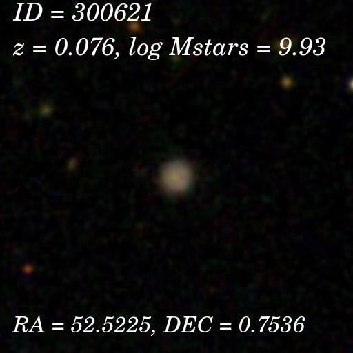
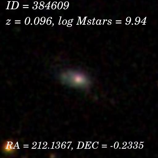
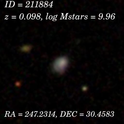
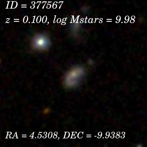
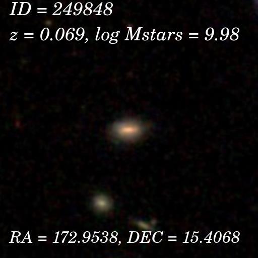
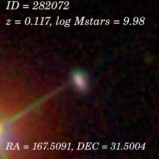
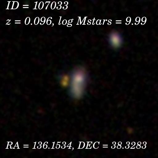
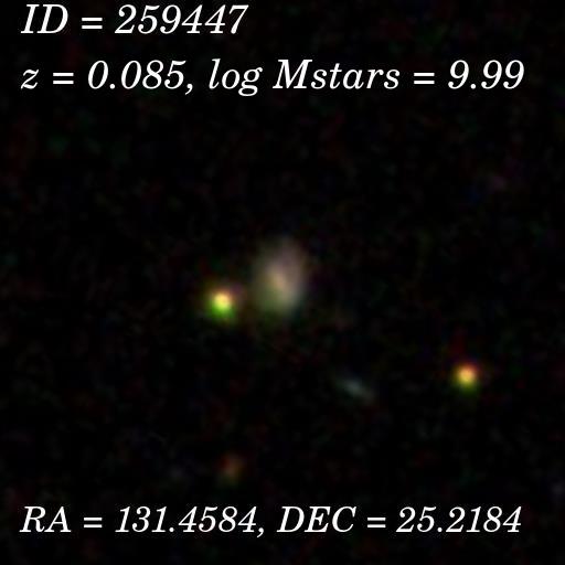
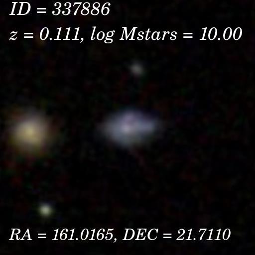
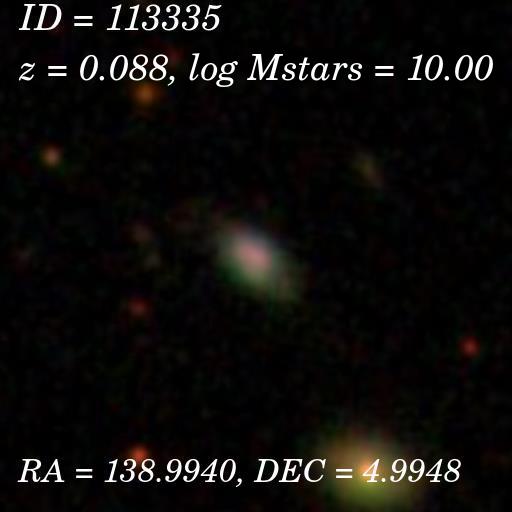
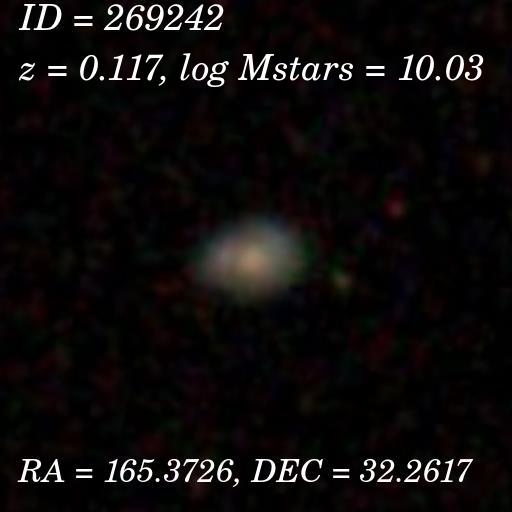
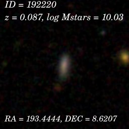
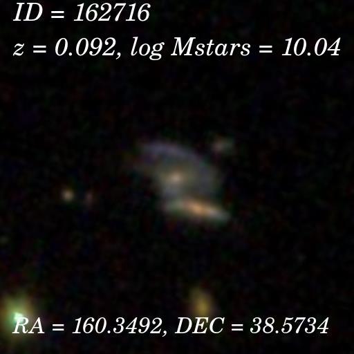
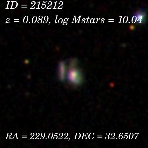
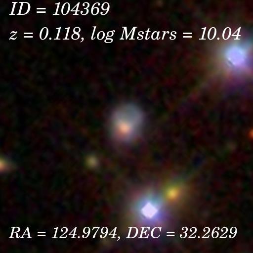
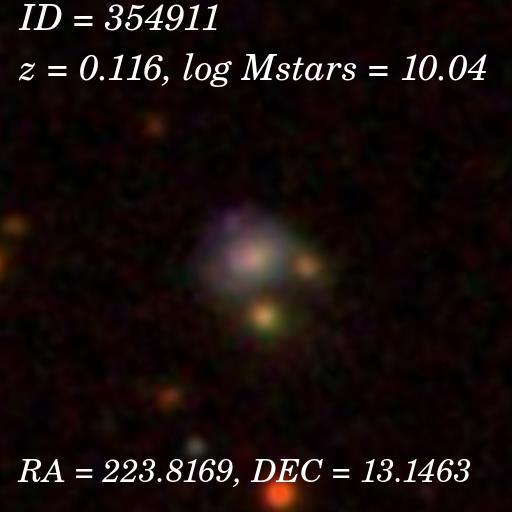
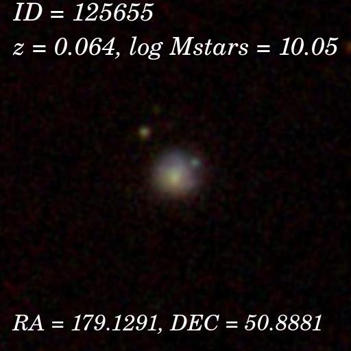
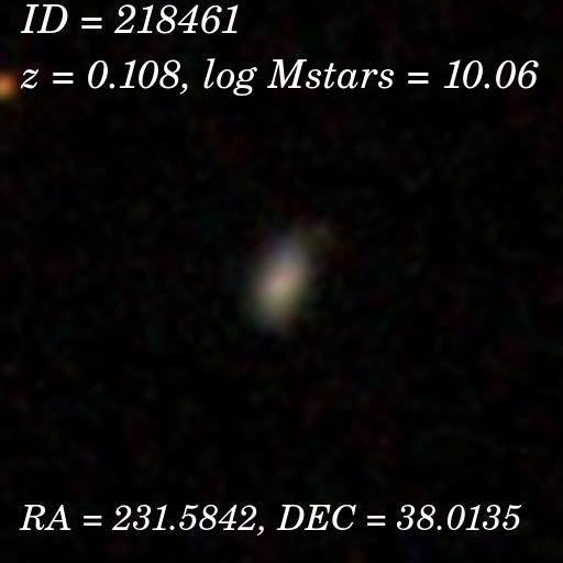
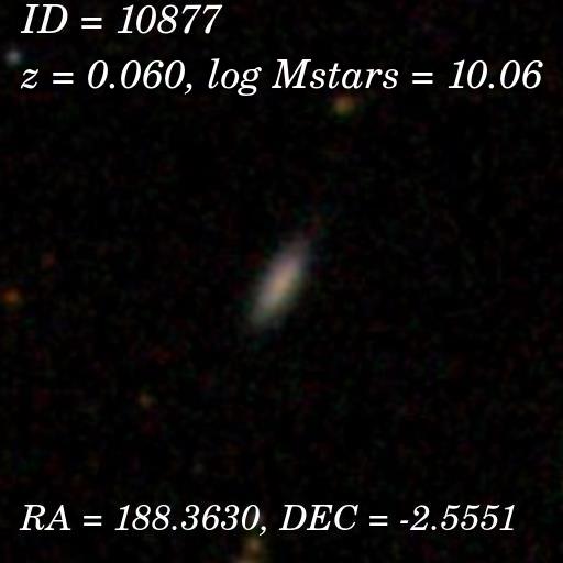
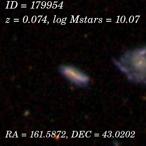
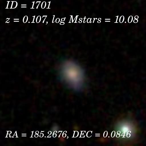
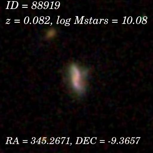
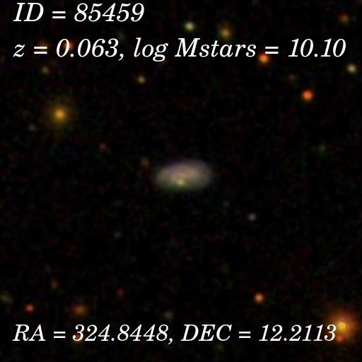
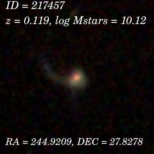
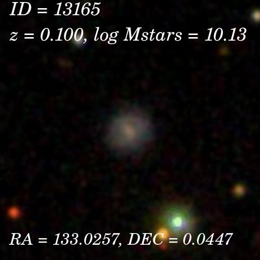
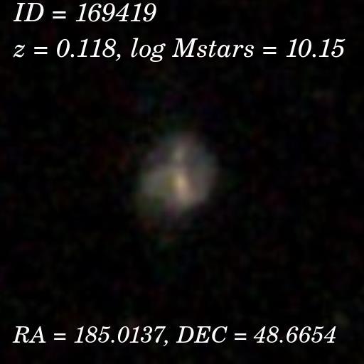
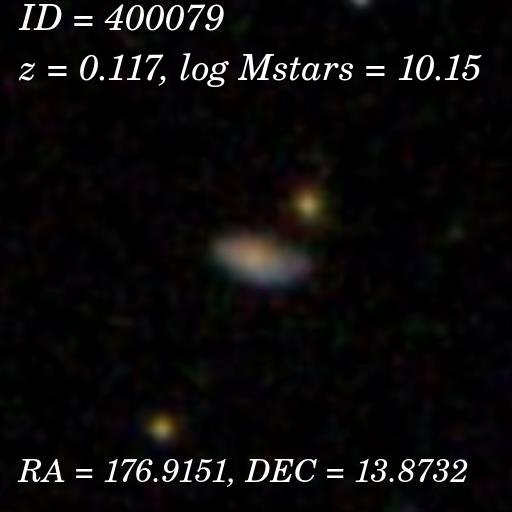
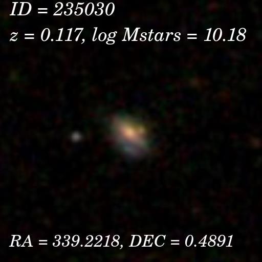
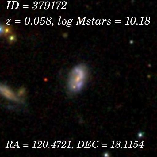
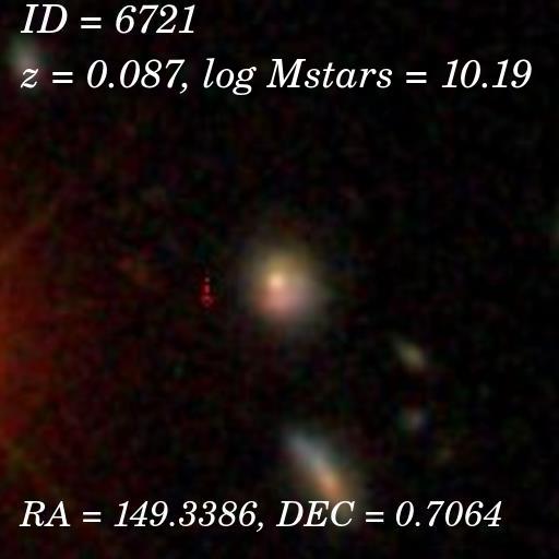
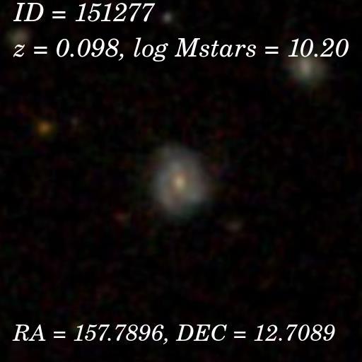
Figure 26: SDSS images of a sample of 207 VYGs. All images are 100 x 100 kpc (cont.).

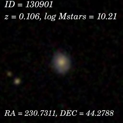
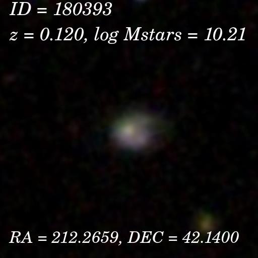
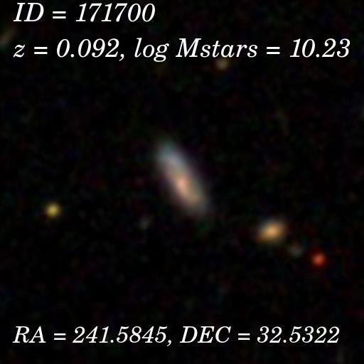
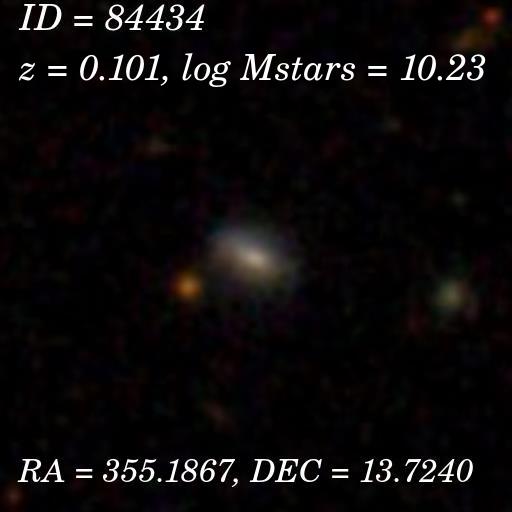
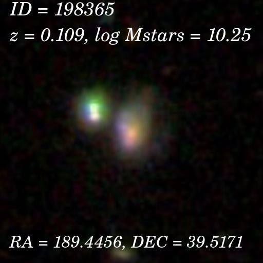
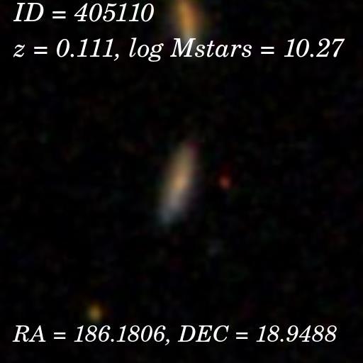
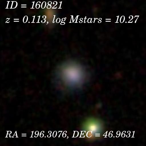
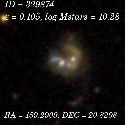
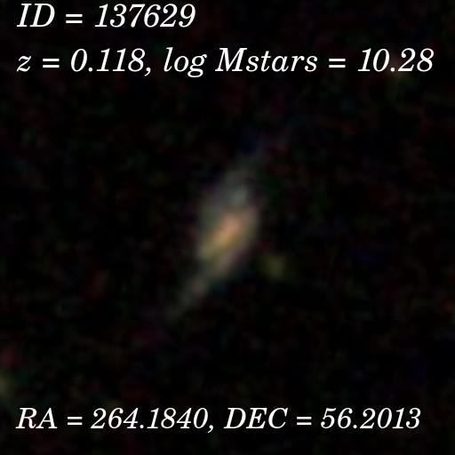
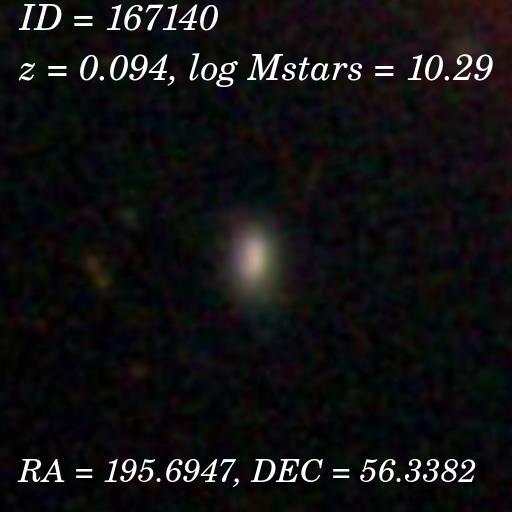
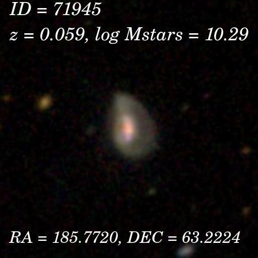
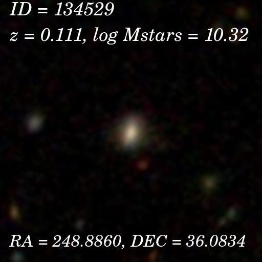
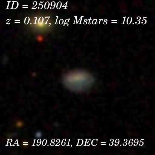
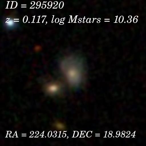
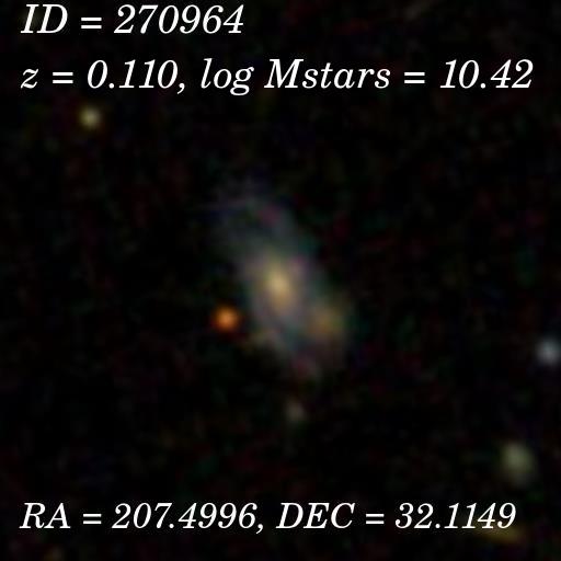
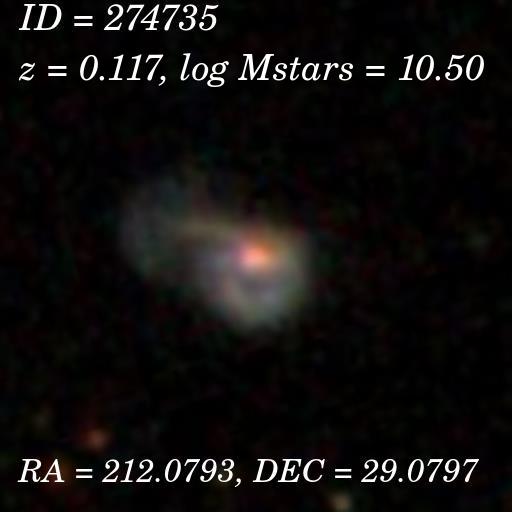
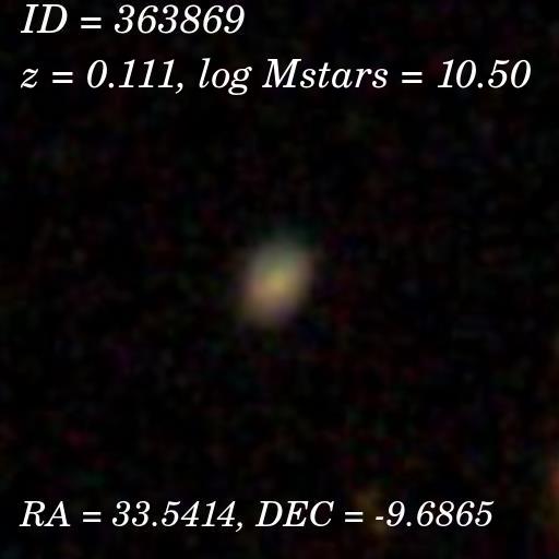
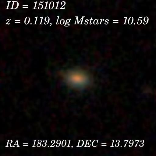
Figure 27: SDSS images of a sample of 207 VYGs. All images are 100 x 100 kpc (cont.).

The high fraction of uncertain classifications in GZ1 indicate that most of our galaxies cannot be simply classified as ellipticals or spirals. Even when discarding galaxies with small angular sizes, the fractions of VYGs and CSGs that are classified as uncertain is very high (61% and 50% of VYGs and CSGs with $\theta_{50}>3^{\prime\prime}$, respectively). The morphological classification by DS18 also points to this conclusion, since only a small fraction of VYGs and CSGs could be reliably classified as one of these two morphological types (15% of spirals with $p_{\rm disk}\geq 0.8$ and 0.5% of ellipticals with $p_{\rm bulge}\geq 0.8$). This is confirmed by examination of Figs. 24–27, which display the VYG images. On the other hand, the distribution of T-types (Fig. 5) is not compatible with irregular morphology, which is characterized by high T-type values ($9-10$). However, the range of T-types values in the DS18 catalogue goes from $\sim-3$ to $\sim 6$, and only 0.4% of the galaxies have T-type values greater than 6 (2861 out of 670 722 galaxies).

To understand what morphological types these T-type values correspond to, we used the parameter gz2_class from GZ2 to select elliptical, spiral and irregular galaxies and analysed the T-type distributions of these three morphological classes. The gz2_class parameter is a string that indicates the most common consensus classification for the galaxy, and is composed by the letter E (galaxies that are smooth) or S (galaxies with disks and/or features), followed by other letters indicating several galaxy features (see the Appendix in Willett et al., 2013 for details). We assumed to be ellipticals all galaxies with gz2_class$\,=\,$Er or Ei, where the letters ‘r’ and ‘i’ indicate that the galaxy is round or in-between round and cigar-shaped. We used the classification for bulge prominence as an indication for spiral morphology, and to avoid selecting lenticulars, we selected galaxies with no bulge or systems for which the bulge is just noticeable (gz2_class$\,=$SBc+, SBd+, Sc+, or Sd+, where ‘+’ indicates other features). The same selection was made for the irregulars, but gz2_class contains the identifier for irregular morphology ‘(i)’, i.e., gz2class = Sc+(i), SBc+(i), Sd+(i), SBd+(i).

Fig. 6 shows that the VYG and CSG T-type distributions (Fig. 6a) are similar to that of irregulars, as seen in Fig. 6b. The irregulars have median T-type = 4.7, and the 10th and 90th percentiles are 2.4 and 5.8. The spirals have lower T-types, with median 3.0, and 10th and 90th percentiles of -0.7 and 4.8. The median of the VYG and CSG T-type values are 4.4 and 4.3, respectively, with 10th and 90th percentiles of 1.2 and 5.6 (VYGs) and 2.2 and 5.5 (CSGs). As already indicated in the results shown in Fig. 5, the we find an excess of VYGs with small T-types, and the number of VYGs with negative values is 3.2 times higher than the number of CSGs with T-type$\,<0$ (5.9% of the VYGs and 1.9% of the CSGs). Fisher’s (Fisher, 1935) and Barnard’s (Barnard, 1945) tests, performed using the R packages stats (R Core Team, 2015) and Barnard (Erguler, 2016), indicate that this difference between the VYG and CSG early-type fractions is statistically significant, with $p$-values$\,=0.002$ and $0.03$, respectively. The inspection of the images of these galaxies reveals that both VYGs and CSGs with negative T-types have spheroid-like morphology, but VYGs spheroids are bluer than the CSGs spheroids, with median $g-i$ colours of 0.7 (VYGs) and 0.9 (CSGs).

Parametric models of bulges and/or disks may not give a good representation of these systems. So, to obtain more information and characterize the galaxy morphology, we have adopted a non-parametric approach. We used the popular CAS system (concentration, asymmetry and clumpiness) presented in Abraham et al. (1994); Abraham et al. (1996) and Conselice, Bershady & Jangren (2000).

We measured the concentration as the ratio of radii containing 90 and 50 per cent of the Petrosian flux in the $r$ band, $\theta_{90}/\theta_{50}$, which we retrieved from the SDSS-DR12 database as petroR90_r and petroR50_r, respectively.

We also compute the galaxy surface brightness as

$$\mu_{50}=m_{r}-k_{0.1}+2.5\log(2\pi\theta_{50}^{2})-10\log(1+z)$$ (1)

where $m_{r}$ is the extinction-corrected Petrosian magnitude in the $r$ band, $k_{0.1}$ is the $k$-correction, and $\theta_{50}$ is the radius (in arcsec) containing 50% of the Petrosian flux in the $r$ band. The $k$-correction was obtained with the code kcorrect with the SDSS filters shifted to $z=0.1$

The galaxy asymmetry and clumpiness were measured using Morfometryka (Ferrari et al., 2015), which is a code to perform structural and morphometric measurements on galaxy images. The asymmetry coefficient is determined by comparing the galaxy image with a rotated version of itself. Three different asymmetry estimates are computed by the code. Here we adopt the standard one defined by Abraham et al. (1996), $A_{1}$, with the difference that we do not subtract the background asymmetry, since this procedure leads to an unstable estimate of the coefficient $A_{1}$ and makes it dependent of the region selected to measure the sky asymmetry. Instead, only the region within the Petrosian radius is used.

Similarly, Morfometryka also computes three different clumpiness coefficients (confusingly denoted “smoothness” and denoted by $S_{1}$ and $S_{2}$, even though higher $S_{i}$ values correspond to more clumpy distributions) by comparing the galaxy image with a smoothed version of itself. In this work we adopt $S_{1}$ defined by Lotz, Primack & Madau (2004) using a Hamming window (Hamming, 1998) with size $\theta_{\rm Petro}/4$, where $\theta_{\rm Petro}$ is the galaxy Petrosian radius.

Although the Morfometryka code returns many other parameters, including modified versions of asymmetry and clumpiness as described in detail in Ferrari et al. (2015), we show only $A_{1}$ and $S_{1}$ because they are less dependent on the S/N of the images. In particular, the Gini and M20 parameters, which are an extension of the CAS system (Lotz et al., 2004), are also measured by Morfometryka. However, we found them to be very dependent on the S/N of the image. Besides, it is not straightforward to physically interpret the Gini and M20 parameters.

All the Morfometryka fits were visually inspected, and we excluded 27 (13%) VYGs and 132 (11%) CSGs with fits affected by foreground stars or very close objects (distances $\mathrel{\hbox{\hbox to0.0pt{\hbox{\lower 4.0pt\hbox{$\sim$}}\hss}\hbox{$<$}}}5^{\prime\prime}$).

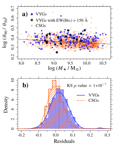
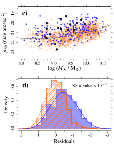
Figure 7: Top: Concentration (left) and surface brightness (right) of VYGs (blue circles) and normal galaxies (orange symbols). The VYGs with EW(H$\alpha$)$\,\geq 150\,$Å are indicated by the black crossed circles. The solid lines in both panels correspond to a second-order polynomial fit to the concentration and $\mu_{50}$ vs. stellar mass relations for galaxies in the control sample. Bottom: Distribution of residuals from the second-order polynomial fit for the VYG (blue histograms) and control (orange) samples. In each panel, we indicate the $p$-value of KS tests.

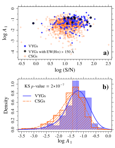
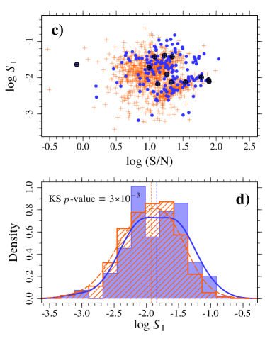
Figure 8: Top: Asymmetry ($A_{1}$) and clumpiness ($S_{1}$) parameters as a function of signal-to-noise ratio. The notation is the same as in Fig. 3. Bottom: Distribution of $\log A_{1}$ and $\log S_{1}$ for the VYG (blue histograms) and control (orange) samples. In each panel, we show the KS test $p$-values.

In Fig. 7, we show the galaxy concentration (panel a) and surface brightness (panel c) as a function of the stellar mass. The residuals derived from fitting the data show that the VYGs are more concentrated and have higher surface brightness than normal galaxies (Figs. 7b,d). The KS tests indicate that these results have high statistical significance, with $p=10^{-7}$ (concentration) and $p<10^{-10}$ (surface brightness).

Since the structural parameters, such as asymmetry and clumpiness, may be sensitive to the S/N of the images, we show in Fig. 8a,c the $A_{1}$ and $S_{1}$ parameters as a function of the signal-to-noise ratios instead of stellar masses. We confirm the weak dependency of of $A_{1}$ with S/N, with Kendall and Spearman correlation coefficients $\tau=0.02$ and $\rho=0.03$. On the other hand, $S_{1}$ shows an anti-correlation with S/N ($\tau=-0.11$ and $p$-value$=2\times 10^{-9}$; $\rho=-0.17$ and $p$-value$=8\times 10^{-11}$). In summary, the comparison between the $S_{1}$ distributions of the VYGs and control samples should be considered with caution. The distributions of these parameters are shown in panels b and d. We can see that the VYGs tend to be more asymmetric and clumpy when compared to normal galaxies, with high statistical significance ($p=2\times 10^{-7}$ for the asymmetry parameter and $p=3\times 10^{-3}$ for the clumpiness). In Fig. 8 we show only galaxies with good Morfometryka fits, i.e., galaxies with nearby objects (in projection) affecting the estimate of the structural parameters are excluded from the plots (27 VYGs and 132 CSGs, corresponding to 13% and 11%, respectively).

To obtain meaningful structural parameter measurements, the angular size of the galaxy must be greater than the resolution of the SDSS image and the atmospheric seeing. It can be seen in Fig. 1d that many of our galaxies have small angular sizes and might be unresolved. However, we note that, since the VYG and CSG $\theta_{50}$ distributions are similar by construction, differences between the VYG and CSG structural parameters are unlikely to arise from differences in the angular sizes of galaxies in these two samples.

4 Ionized gas, neutral gas and dust content

4.1 Oxygen abundances of the ionized gas

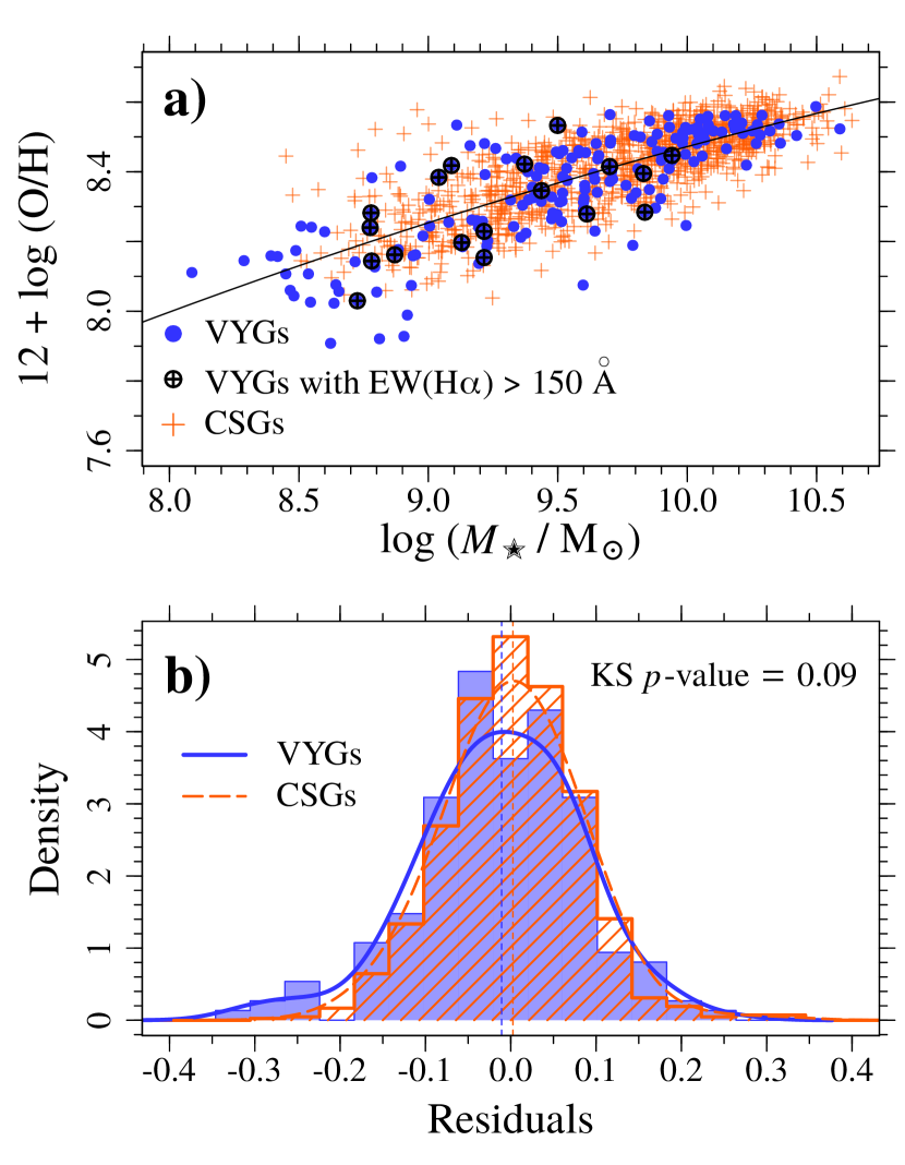
Figure 9: Ionized gas oxygen abundances as a function of stellar mass. The abundances were derived using emission line fluxes from the SDSS table GalSpecLine (MPA-JHU). The notation is the same as in Fig. 3. The bottom panel shows the distribution of residuals from the second-order polynomial fit for the VYG (blue histograms) and control (orange) samples.

The gas oxygen abundance, an indicator of metallicity, was derived from the emission-line fluxes retrieved from the SDSS database. Two sets of measurements are available: one given by the MPA-JHU catalogue (table galSpecLine in SDSS DR12, Brinchmann et al., 2004; Tremonti et al., 2004) and the other by the catalogue of the Portsmouth group (table emissionLinesPort in SDSS DR12). The first one employs the Bruzual & Charlot (2003) models to fit the stellar continuum, while models from Maraston & Strömbäck (2011) and Thomas, Maraston & Johansson (2011) are used in the Portsmouth measurements. The use of line measurements from two different catalogues allows to estimate the uncertainties in the abundances of the target galaxies due to uncertainties in the line flux measurements.

We extracted from those catalogues the measurements of the [O ii]$\lambda$3727, [O ii]$\lambda$3729, H$\beta$, [O iii]$\lambda$4959, [O iii]$\lambda$5007, [N ii]$\lambda$6548, H$\alpha$, [N ii]$\lambda$6584, [S ii]$\lambda$6717, and [S ii]$\lambda$6731 emission lines in the spectra. We restricted our analysis to galaxies whose emission lines were measured with S/N$\,>3$ for all lines. We corrected the emission line fluxes for interstellar reddening using the observed H$\alpha$/H$\beta$ ratio and the reddening function from Cardelli, Clayton & Mathis (1989) for $R_{V}=3.1$, which leads to $A_{{\rm H}{\beta}}=1.164\,A_{V}$.

The “direct $T_{e}$” method (e.g., Dinerstein, 1990) is believed to provide the most reliable abundance determinations in SF regions from the emission lines in their spectra. However, it requires high-precision spectroscopy to detect weak auroral lines such as [O iii]$\lambda$4363 and [N ii]$\lambda$5755. Unfortunately, these auroral lines are usually not detected or they are measured with a large uncertainty in the SDSS spectra. The abundances in SDSS objects with emission line spectra are thus usually estimated using "the strong line method" of Alloin et al. (1979) and Pagel et al. (1979), using intensity ratios of the strong emission lines in the spectra.

Two families of calibrations are widely used. The family of the calibrations following Pagel et al. (1979) is based on the oxygen lines. Both 1D (e.g. Zaritsky, Kennicutt & Huchra 1994; Tremonti et al. 2004) and 2D (or parametric, $p$-method) calibrations (Pilyugin, 2000, 2001; Pilyugin & Thuan, 2005) have been suggested. The family of the calibrations following Alloin et al. (1979) is based on the nitrogen lines. There are only 1D calibrations of this kind for abundance determinations in high metallicity objects (e.g. Pettini & Pagel, 2004; Marino et al., 2013). There is no unique relation applicable across the whole range of metallicities of H ii regions. Instead, distinct calibration relations are constructed for high (upper branch) and low metallicities (lower branch). But these branches are not applicable to objects lying in the transition zone (e.g. Pilyugin & Thuan, 2005, and discussion there). Moreover, to choose the relevant calibration relation, one has to know a priori to which interval of metallicity the H ii region belongs. A wrong choice would lead to a wrong abundance. Many of our galaxies may have moderate to low metallicities, i.e. they belong to the transition zone and to the lower branch, making abundance determinations for our objects particularly difficult.

We used the simple 3D calibration relations proposed by Pilyugin & Grebel (2016). The oxygen abundances (O/H)_R are determined using the $R$ calibration, i.e., (O/H)_R = $f$(R₂, R₃, N₂), where the oxygen R₂, R₃ and the nitrogen N₂ lines are given by

$$R_{2} = I_{\rm[O\,II]\lambda 3727+\lambda 3729}/I_{{\rm H}\beta},$$

$$R_{3} = I_{{\rm[O\,III]}\lambda 4959+\lambda 5007}/I_{{\rm H}\beta},\ {\rm and}$$

$$N_{2} = I_{\rm[N\,II]\lambda 6548+\lambda 6584}/I_{{\rm H}\beta}.$$

One advantage of this calibration is that it is applicable over the entire metallicity range of H ii regions. Although distinct relations for high- and low-metallicity objects are constructed, the separation between these two can be simply obtained from the intensity of the $N_{2}$ line. Moreover, the applicability ranges of the high- and low-metallicity relations overlap, making the transition zone disappear.

Since the [O iii]$\lambda$5007 and $\lambda$4959 lines originate from transitions from the same energy level, their flux ratio is determined only by the transition probability ratio, close to 3 (Storey & Zeippen, 2000). Therefore, the value of $R_{3}$ can be estimated as $R_{3}=I_{{\rm[O\,III]}\lambda 4959+\lambda 5007}/I_{{\rm H}\beta}$ or $R_{3}=1.33I_{{\rm[O\,III]}\lambda 5007}/I_{{\rm H}\beta}$. The stronger line [O iii]$\lambda$5007 is usually measured with higher precision than the weaker line [O iii]$\lambda$4959. We thus used the latter expression to calculate $R_{3}$, instead of the sum of the [O iii] line fluxes. The same applies to the nitrogen lines [N ii]$\lambda$6584 and $\lambda$6548. They also originate from transitions from the same energy level and the transition probability ratio for those lines is again close to 3 (Storey & Zeippen, 2000). We again calculate $N_{2}$ as $N_{2}=1.33$ [N ii]$\lambda$6584/H$\beta$, instead of using the sum of the [N ii] lines.

The radiation of the diffuse ionized gas is believed to contribute significantly to some fibre SDSS spectra, and may increase the strength of the low-ionization lines [N ii], [O ii], and [S ii] relative to the Balmer lines. If this is the case, then the abundances derived from the SDSS spectra by strong-line methods may have large errors (Belfiore et al., 2015, 2017; Zhang et al., 2017; Sanders et al., 2017). Pilyugin et al. (2018). found that the mean increase of R₂ and N₂ is less than a factor of $\sim 1.3$, and the $R$ calibration produces reliable abundances.

For each galaxy in our sample with an available oxygen line R₂ and a S/N greater than 3 for the emission lines of interest, we have determined two values of the oxygen abundance, one based on the MPA-JHU line measurements and the other on the Portsmouth ones. We have found that the two sets of abundances are in excellent agreement ($\Delta=0.005\pm 0.02\,$dex). Hence, we only present here the results based on the MPA-JHU catalogue.

In Fig. 9a, we show how the VYG and CSG oxygen abundances vary with galaxy stellar mass. Only galaxies with good MPA-JHU emission-line measurements (i.e., S/N$\,\geq 3$) are shown (183 VYGs and 1031 CSGs, corresponding to $88\%$ and $83\%$ of the galaxies in these samples, respectively). We fitted the $12+\log({\rm O/H})$ vs. $\log(M_{\star}/{\rm M}_{\odot})$ relation of the CSG, and show the distribution of residuals for both samples in Fig. 9b. The residuals from the fit indicate that there is no significant difference between the oxygen abundances of the VYGs and the CSGs as a function of stellar mass (KS test $p$-value$\,=0.09$). We also compared the best-fit to the VYG $12+\log({\rm O/H})$ vs. $\log(M_{\star}/{\rm M}_{\odot})$ relation to that of the CSGs, and find that the difference between the two fits does not exceed 0.015 dex within the range $8.0\leq\log(M_{\star}/{\rm M}_{\odot})\leq 10.6$. Using a first-order polynomial to fit the VYG and CSG relations, we also get very similar slopes for both samples (0.23 and 0.22 for the VYGs and CSGs, respectively).

On the other hand, when we limited our analysis to galaxies with $M_{\star}\leq 10^{9}\,{\rm M}_{\odot}$, we found that low-mass VYGs have lower oxygen abundances by 0.07 dex, on average, compared to those of the CSGs, with a KS test indicating marginal statistical significance ($p$-value$\,=0.02$). But a large fraction of the low-mass CSGs are excluded from this analysis when we require emission-line measurements with S/N$\,\geq 3$. Among the 210 CSGs with $M_{\star}\leq 10^{9}\,{\rm M}_{\odot}$, only 78 ($37\%$) pass the S/N criteria, while $73\%$ of the VYGs within the same mass range have good line-emission measurements (36 out of 49). The higher sSFRs of low-mass VYGs compared to the those of the CSGs might explain why a larger fraction of low-mass CSGs is excluded from our analysis of the oxygen abundances. Galaxies with higher sSFRs have stronger emission lines which result in flux measurements with higher S/N ratios. Therefore, the selection effects introduced by this cut in S/N affects the low-mass VYG and CSG samples differently, and the comparison between their oxygen abundances must be seen with caution.

Finally, there are 6 low-metallicity VYGs with oxygen abundances $3\,\sigma$ below the $\log({\rm O/H}+12)$ vs. stellar mass relation: they have lower metallicities for their stellar masses. However, this result is not statistically significant.

4.2 Neutral hydrogen content

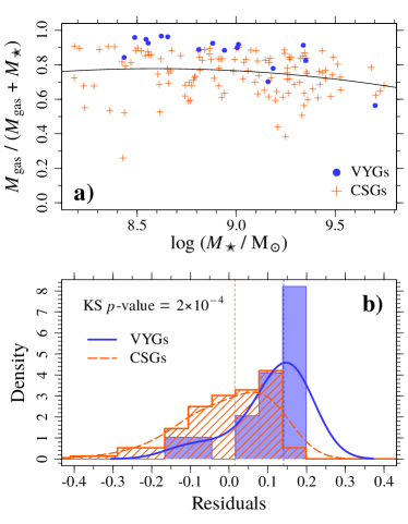
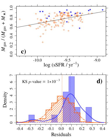
Figure 10: Fraction of atomic gas in galaxies with H i detections in the ALFALFA survey as a function of galaxy stellar mass (upper left) and $\log({\rm sSFR})$ (upper right). The residuals from the linear fits to the CSG $f_{\rm HI}$ vs. stellar mass and vs. $\log({\rm sSFR})$ relations are shown in the bottom panels. The blue and orange histograms correspond to the VYG and CSGs, respectively and, in each panel, we indicate the $p$-values of the KS tests.

The atomic gas content of our galaxies was investigated using the data from the Arecibo Legacy Fast ALFA (ALFALFA) survey (Haynes et al., 2011, 2018). The ALFALFA H i source catalogue contains $31\,502$ detections, and approximately half of our objects lies in the ALFALFA-SDSS overlap region ($\sim 4000\,$deg²). The coordinates of the most probable optical counterpart (OC) of each H i detection are available in the catalogue. We cross-matched our VYG and CSG samples by adopting a maximum angular separation of $5^{\prime\prime}$ between the OC and the SDSS galaxy. We found 149 galaxies with H i detections, among which 19 are VYGs and 130 are CSGs, corresponding to $9.2\%$ and $10.5\%$ of these samples, respectively. For each galaxy, we computed the atomic gas mass fraction $f_{\rm gas}$, i.e., the gas mass divided by the sum of the gas and stellar masses, $f_{\rm gas}=M_{\rm gas}/(M_{\rm gas}+M_{\star})$. We accounted for the He gas by assuming that the total gas mass satisfies the relation $M_{\rm gas}=1.33\,M_{\rm H\textsc{i}}$. The stellar masses were obtained from our SPS analysis, using the V15 spectral model with STARLIGHT.

Measurements of H i masses may be contaminated by the neutral gas of nearby galaxies because of the large Arecibo beam size (FWHM$\,=3.5\,$arcmin). We checked for such neighbour contamination by using the SDSS spectroscopic catalogue to identify the VYGs and CSGs that have other galaxies within a radius of $1.8\,$arcmin ($\sim 90$% of the beam flux) and $\Delta z\leq 2\,W_{20}/c$, where $W_{20}$ is the velocity width of the H i line profile in km s^-1, measured at the 20% level of of each of the two peaks on the low- and high-velocity horns of the profile (see Springob et al., 2005) and $c$ is the speed of light. Although this procedure misses galaxies fainter than the magnitude limit of the SDSS spectroscopic observations ($m_{r}\leq 17.77$), we use the spectra to estimate the total stellar mass within the Arecibo beam. The stellar masses of the nearby galaxies were computed using the STARLIGHT code with the V15 spectral models as described in Sect. 2.

We found that 3 VYGs and 5 CSGs ($15.8\%$ and $3.8\%$, respectively) have other galaxies at distances $\leq 1.8\,$arcmin and within the $\Delta z$ limit described above. The fraction of VYGs with nearby galaxies is 4.1 times higher than that of the CSGs. However, the stellar masses of the galaxies around the VYGs are lower than those of galaxies in the CSG surroundings. The total stellar mass within the beam is $0.26\,$dex higher (median) than the mass of the VYGs, while for the CSGs, the total mass is $\sim 0.9\,$dex higher (median). The median gas fraction computed with the total stellar mass within the beam, $M_{\rm gas}/(M_{\rm gas}+M_{\star,\rm beam})$, is 0.88 and 0.66 for these VYGs and CSGs, respectively. When comparing these values with the median gas mass fractions of VYGs and CSGs with no nearby galaxies within $1.8\,$arcmin ($\langle f_{\rm gas}\rangle=0.91$ and $0.76$, respectively) , we see that the CSG gas fractions are more affected by nearby galaxies. Therefore, we conclude that the presence of other galaxies does not lead to higher VYGs gas fractions compared to the CSGs.

In Fig. 10 we show how $f_{\rm gas}$ varies with galaxy stellar mass (Fig. 10a) and sSFR (Fig. 10c). The 3 VYGs and 5 CSGs that have nearby galaxies within the Arecibo beam, identified as described above, are excluded from the plot. For a given stellar mass and sSFR, the fraction of atomic gas in VYGs is systematically larger compared to the one in CSGs. About $80\%$ of the VYGs with H i detections and no nearby galaxies (13 out of 16 VYGs) have $f_{\rm gas}>0.8$, while only $42\%$ of the CSGs have such high gas mass fractions (52 out of 125 CSGs). We fitted the CSG $f_{\rm gas}$ vs. stellar mass and vs. $\log({\rm sSFR/yr^{-1}})$ relations, and found that 14 out of 16 VYGs ($87.5\%$) lie above the best-fit relation. The KS tests applied to the distributions of the residuals provide $p$-values$\,=2\times 10^{-4}$ and $1\times 10^{-3}$ (Figs. 10b,d).

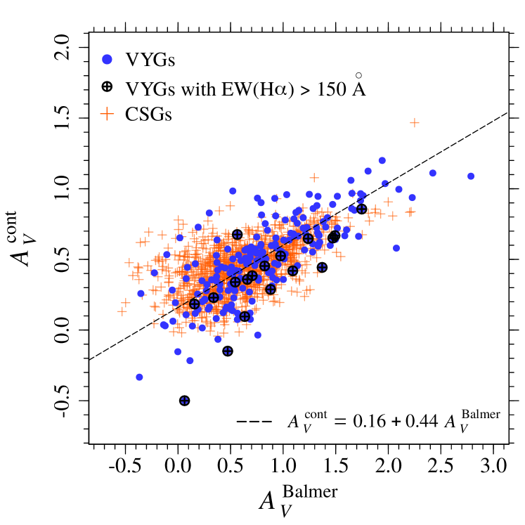
Figure 11: Internal extinction estimated from spectral fitting analysis using STARLIGHT vs. extinction obtained from the Balmer decrement. The notation is the same as in Fig. 3. The dashed line indicates the relation $A_{V}^{\rm cont}=0.16+0.44\,A_{V}^{\rm Balmer}$, which is the relation found by Calzetti et al. (2000) plus an offset of $0.16$ magnitudes.

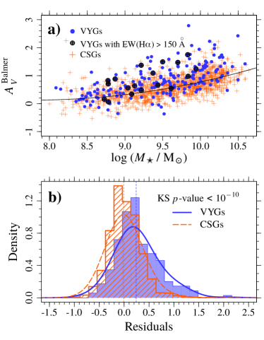
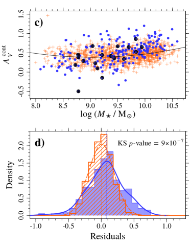
Figure 12: Top: Internal extinction estimated from the Balmer decrement (left) and from spectral fitting analysis using STARLIGHT (right), both as a function of stellar mass. The solid lines in both panels indicate the second-order polynomial fits to the $A_{V}^{\rm Balmer}$ and $A_{V}^{\rm cont}$ vs. stellar mass relations. The notation is the same as in Fig. 3. Bottom: Residuals from the second-order polynomial fit for the VYG (blue histograms) and control (orange) samples.

The gas mass fractions of VYGs are $\sim\,$20% higher than those in CSGs. These large values might be due to the fact that VYGs have not managed to convert the neutral gas into stars before the last Gyr. We explore in the next section whether environmental effects can be the cause of that delayed SF.

It is important to note that the gas mass fractions and the properties inferred from the SDSS spectra are measured within different volumes of the galaxy, since the ALFALFA beam is $\sim 70$ times the size of the SDSS fibre.

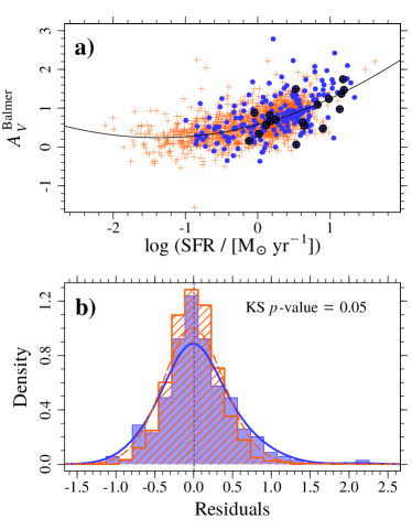
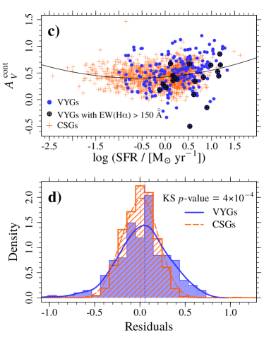
Figure 13: Top: Internal extinction estimated from the Balmer decrement (left) and from spectral fitting analysis using STARLIGHT (right), both as a function of the star formation rate. The solid lines in both panels indicate the second-order polynomial fits to the $A_{V}^{\rm Balmer}$ and $A_{V}^{\rm cont}$ vs. $\log{\rm SFR}$ relations. The notation is the same as in Fig. 3. Bottom: Residuals from the second-order polynomial fit for the VYG (blue histograms) and control (orange) samples.

4.3 Dust content and internal extinction

We estimated the amount of dust in our galaxies using two measures. We first derived the extinction in the $V$ band, $A_{V}^{\rm cont}$, from the SPS analysis using the V15 spectral model with STARLIGHT and assuming the Cardelli, Clayton & Mathis (1989) reddening law. We also measured the dust extinction from the Balmer decrement, $A_{V}^{\rm Balmer}$, which is inferred from the ratio of the H$\alpha$ and H$\beta$ emission-line fluxes $F_{{\rm H}\alpha}/F_{{\rm H}\beta}$. This ratio should be 2.87 in the case of no extinction and a temperature $T=10\,000\,\rm K$ (Savage & Mathis, 1979). To derive $A_{V}^{\rm Balmer}$, we first compute the the colour excess $E(B-V)$ given by (see, e.g., Momcheva et al., 2013; and Domínguez et al., 2013 for details)

$$E(B-V)=\frac{2.5}{k(\lambda_{{\rm H}\beta})-k(\lambda_{{\rm H}\alpha})}\log\left[\frac{F_{{\rm H}\alpha}}{2.87\,F_{{\rm H}\beta}}\right]\ .$$

where $k(\lambda_{{\rm H}\beta})$ and $k(\lambda_{{\rm H}\alpha})$ are the values of the reddening curves at H$\beta$ and H$\alpha$ wavelengths, respectively. The factor $2.5/[k(\lambda_{{\rm H}\beta})-k(\lambda_{{\rm H}\alpha})]=2.33$ for the Cardelli, Clayton & Mathis, 1989 reddening law. The extinction in the $V$ band is then computed as $A_{V}^{\rm Balmer}=R_{V}\,E(B-V)$, with $R_{V}=3.1$.

We compared the two extinction estimates in Fig. 11, and it can be seen that $A_{V}^{\rm Balmer}$ tend to be greater than $A_{V}^{\rm cont}$. This result has been already found in previous studies (e.g., Calzetti et al., 2000; Asari et al., 2007; Kreckel et al., 2013; Florido et al., 2015) and suggests that $A_{V}^{\rm Balmer}$ and $A_{V}^{\rm cont}$ are probing dust in different components of the galaxy ISM. The $A_{V}^{\rm Balmer}$ value is dominated by dust absorption within molecular clouds in active star-forming regions, while the reddening of the stellar continuum is mainly due to absorption by dust distributed more homogeneously through the galaxy ISM. The slope of the relation between $A_{V}^{\rm Balmer}$ and $A_{V}^{\rm cont}$ found by Calzetti et al. (2000) for starburst galaxies is consistent with our measurements, as indicated by the line shown in Fig. 11. However, we find an offset of $0.16$ magnitudes relative to the Calzetti et al. relation, which might be due to more diffuse dust in our galaxies compared to the starburst galaxies studied by these authors.

In Figs. 12a,c, we show $A_{V}^{\rm Balmer}$ and $A_{V}^{\rm cont}$ as a function of stellar mass for the VYGs and CSGs. We fitted the $A_{V}^{\rm Balmer}$ and $A_{V}^{\rm cont}$ vs. $\log M_{\star}$ relations for the CSGs and the residuals from these fits are shown in Figs. 12b,d. The VYGs have systematically higher internal extinctions, with KS tests indicating high statistical significance ($p$-values $<10^{-6}$). However, Figs. 12a,c suggest that the higher dust content of VYGs relative to CSGs is most pronounced at high galaxy masses and is nonexistent ($A_{V}^{\rm Balmer}$) or reversed ($A_{V}^{\rm cont}$) at low masses. We will discuss the differences between the VYGs and CSGs in the high- and low-mass regimes in Sect. 6.4.

The amount of light absorbed in the interstellar medium depends on the size, geometry and inclination of the galaxy. By construction, the distribution of the CSG physical sizes is close to that of the VYGs, since the angular sizes and redshifts were included in the matching procedure to construct the control sample, leading to similar $\theta_{50}$ vs. $z$ distributions shown in Fig. 2c. In any event, we compared the VYG and CSG $A_{V}^{\rm Balmer}$ and $A_{V}^{\rm cont}$, both normalized by galaxy radius: $A_{V}^{\rm Balmer}/R_{50}$ and $10^{-0.4\,A_{V}}/R_{50}$. After fitting the normalized quantities vs. stellar mass relations and analysing the residuals, we still find significantly higher extinction in VYGs, with KS $p$-values$\,=2\times 10^{-8}$ (for $A_{V}^{\rm Balmer}/R_{50}$) and $2\times 10^{-7}$ (for $10^{-0.4\,A_{V}}/R_{50}$).

We assessed the dependency of the internal extinction on the galaxy geometry and inclination by using the minor-to-major axis ratio $b/a$ as a proxy for these properties. Admittedly, this is a very simplified approach, given the complexity of the ISM structure and geometry, but the detailed characterization of the dust content of the ISM is beyond the scope of this paper. We find that $A_{V}^{\rm cont}$ increases with decreasing $b/a$, as expected if $b/a$ indicates the inclination of disk galaxies. The Kendall and Spearman tests show that this anti-correlation is statistically significant, with coefficients $\tau=-0.15$ and $\rho=-0.22$, and $p$-values$\,<10^{10}$ for both tests. On the other hand, $A_{V}^{\rm Balmer}$ does not show any dependency with the axis ratio, with Kendall $\tau=0.03$ and Spearman $\rho=0.04$ ($p$-values$\,=0.12$ and $0.13$). The difference in the behaviour of $A_{V}^{\rm cont}$ and $A_{V}^{\rm Balmer}$ with galaxy inclination reinforces the idea that they are probing dust in different components of the galaxy ISM.

After taking into account the dependency of $A_{V}^{\rm cont}$ with $b/a$ by fitting the relation for the CSGs and analysing the residuals, the VYGs still have more extinction, with KS $p$-values$\,=1\times 10^{-5}$ (for $A_{V}^{\rm Balmer}$) and $5\times 10^{-6}$ (for $A_{V}^{\rm cont}$). Therefore, the differences between $A_{V}^{\rm Balmer}$ and $A_{V}^{\rm cont}$ of VYGs and CSGs do not appear to be due to distinct sizes, geometries and/or inclination angles, but must be truly related to the amount of dust within these systems, which is significantly higher in VYGs compared to the general population of galaxies.

We extracted the IR magnitudes from the Wide-field Infrared Survey Explorer (WISE, Wright et al. 2010) database, and computed the $r-W1$ and $r-W2$ colours for the VYGs and CSGs, where $W1$ and $W2$ are the WISE bands at 3.4 and 4.6 $\mu$m, respectively. We fitted the $r-W1$ and $r-W2$ vs. stellar mass relations, and the residuals show that VYGs tend to be redder than the CSGs, which is consistent with an excess of dust in VYGs.

The higher amount of dust in VYGs compared to the CSGs may be a consequence of their higher star formation rates (SFR), since there is a correlation between the dust mass and SFR (da Cunha et al., 2010; Hjorth et al., 2014, e.g.). In Fig. 13, we show $A_{V}^{\rm Balmer}$ and $A_{V}^{\rm cont}$ as a function of $\log{\rm SFR}$. Both $A_{V}^{\rm Balmer}$ and $A_{V}^{\rm cont}$ increase with increasing SFR, but the correlation is much stronger for $A_{V}^{\rm Balmer}$. Kendall and Spearman correlation tests confirm the tighter relation between $A_{V}^{\rm Balmer}$ and SFR compared to the $A_{V}^{\rm cont}-\log{\rm SFR}$ relation. We obtained the following coefficients and $p$-values: $\tau=0.45$, $\rho=0.63$, and $p$-value$\,<10^{-15}$ ($A_{V}^{\rm Balmer}-\log{\rm SFR}$ relation); and $\tau=0.08$, $\rho=0.13$, and $p$-value$\,<10^{-5}$ ($A_{V}^{\rm cont}-\log{\rm SFR}$ relation). The different behaviour between $A_{V}^{\rm Balmer}$ and $A_{V}^{\rm cont}$ suggests, again, that they trace the absorption by dust of different ISM components.

As shown in Fig. 13b, after removing the dependency with SFR, we see only a marginally-significant difference between the VYG and CSG $A_{V}^{\rm Balmer}$. This result shows that the amount of dust in VYGs is higher due to their higher SFRs compared to those of CSGs. On the other hand, after taking the $A_{V}^{\rm cont}-\log{\rm SFR}$ relation into account, VYGs have higher $A_{V}^{\rm cont}$ values than CSGs (Fig. 13d). These results suggest that, while the dust mass vs. SFR relations for HII regions in VYGs and CSGs are similar, the amount of diffuse ISM dust in VYGs is higher compared to that of CSGs. Given that VYGs have a significant fraction of $\mathrel{\hbox{\hbox to0.0pt{\hbox{\lower 4.0pt\hbox{$\sim$}}\hss}\hbox{$<$}}}1$ Gyr stellar populations, they are expected to have a large number of TP-AGB stars polluting the ISM with dust. Another possibility is that the timescales for the destruction of the ISM dust by sputtering or other processes are longer than 1 Gyr. We will discuss the VYG and CSG internal extinction and their amount of dust in Sect. 6.6.1.

5 The environment of very young galaxies

If physical processes external to the VYGs are responsible for the recent SF activity, their environment is expected to be different from that of the CSGs. To investigate this possibility, we analyse successively the local, group and large-scale environments of our sample galaxies. We identified possible local effects due to interactions with other galaxies in the immediate surroundings, by searching for neighbours within 200 kpc from each of our sample galaxies. We also visually inspected the galaxy images and classified them according to the presence of tidal features indicating interactions with neighbours or recent mergers. We then characterized the group environment of a galaxy by the halo mass of the group nearest to it and its position within that group, i.e., its distance relative to the group centre. Lastly, we determine the large-scale environment by the position of the galaxies relative to voids and filaments. We describe our approach in detail below.

5.1 Local environment

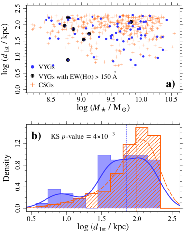
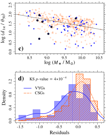
Figure 14: Top: Distance to the closest neighbour galaxy with $m_{r}+1$, where $m_{r}$ is the $r$-band Petrosian magnitude of our galaxies. We show the distances in kpc (left) and normalised by the galaxy radius containing 50% of the Petrosian flux, $\theta_{50}$ (right). We show only galaxies that have a neighbour within $200\,$kpc and that are far ($>200\,$kpc) from bright stars and the borders of the SDSS coverage area (63 VYGs and 392 CSGs). The notation is the same as in Fig. 3. Bottom: Distribution of distances in kpc (left) and the residuals from the linear fit to the normalised distance vs. stellar mass relation of the CSGs (right). The blue and orange histograms correspond to the VYG and control sample, respectively and, in each panel, we indicate the $p$-values of the KS tests.

To investigate the local environment, we have computed for each galaxy in the VYG and control samples the distance to its closest neighbour, as follows. We retrieved from the SDSS-DR12 photometric catalog all galaxies within $200\,$kpc from each of our sample galaxies, not requiring that the neighbour have spectroscopic observations. We adopt this approach because the great majority of the neighbour galaxies do not have listed redshifts in the SDSS. We selected objects with magnitudes $m_{r}+1$, where $m_{r}$ is the extinction-corrected Petrosian magnitude in the $r$ band of our sample galaxy.

We ensured not missing galaxies by requesting that at least 95 per cent of the region within $200\,$kpc from each sample galaxy lies within the SDSS coverage area. For this purpose, we adopted the SDSS-DR7 spectroscopic angular selection function mask provided by the NYU Value-Added Galaxy Catalog team (Blanton et al., 2005), and assembled with the package MANGLE 2.1 (Hamilton & Tegmark, 2004; Swanson et al., 2008). After excluding the galaxies close to bright stars or to the borders of the survey, we get a sample of 883 galaxies, among which 117 are VYGs and 766 are CSGs.

To minimize the contamination by background galaxies, we discard objects with $g-i$ colours $2\,\sigma$ above the red sequence, at the redshift of our sample galaxies. The method used to identify the red sequence at different redshifts is described in Appendix A.

We found that 428 (out of 883) galaxies do not have any neighbour with magnitude $m_{r}+1$ within $200\,$kpc (54 VYGs and 374 CSGs, corresponding to $46.2$% and $48.8$%). Figure 14 shows the distribution of distances to the closest neighbour with magnitude $m_{r}+1$ for the 455 galaxies that have a nearby object at distances $\leq 200\,$kpc. The median distances are $71$ and $98.6\,$kpc for the VYG and control sample, respectively.

We find that 9 out of 117 VYGs (7.7%) have a close companion at distances smaller than 5 times $R_{50}$, while the number for normal galaxies is 22 out of 766 (2.9%). A Barnard’s test indicates that this difference is statistically significant, with a $p$-value$\,=0.02$. These results indicate that the VYGs are more likely to be interacting or merging with nearby galaxies than the control galaxies.

5.2 Interactions and mergers with neighbour galaxies

Table 1: Fractions of VYGs and CSGs that show signs of interactions

Signs of interaction	VYGs	Control	$p$-value
			Fisher	Barnard
(1)	(2)	(3)	(4)	(5)
with neighbours or not	40.6$\pm$3.0%	23.2$\pm$3.8%	0.0002	0.0002
galaxy and neighbour	12.6$\pm$2.0%	6.3$\pm$1.2%	0.04	0.04
galaxy and close neighbour	12.1$\pm$1.8%	6.3$\pm$1.2%	0.06	0.05
with no neighbour	8.2$\pm$1.3%	3.9$\pm$2.5%	0.10	0.09

Besides identifying the closest neighbour, as described above, we have also looked for signs of interactions or features indicating recent merger events. To identify merging systems, we use the classification from the Galaxy Zoo 1 project (Lintott et al., 2011). The method consists in converting a set of visually-inspected classifications by hundreds of thousands of volunteers into a single parameter, $p_{\rm merger}$, which corresponds to the weighted fraction of votes in the “merger” category. Darg et al. (2010) have shown that galaxies with $p_{\rm merger}\mathrel{\hbox{\hbox to0.0pt{\hbox{\lower 4.0pt\hbox{$\sim$}}\hss}\hbox{$>$}}}0.4$ are, in fact, true mergers. Although $p_{\rm merger}$ is certainly related to the probability that a galaxy is part of an ongoing merger, adopting a single critical $p_{\rm merger}$ threshold to classify a galaxy as merging may be over-simplistic.

To avoid choosing a specific threshold, we computed the fraction of VYGs and CSGs that could be classified as merging systems for different $p_{\rm merger}$ threshold values, as shown in Fig. 15. Regardless of the threshold adopted, the fraction of VYGs that are merging is $\sim 2$ times higher than that of the CSGs (KS $p$-value$\,=5\times 10^{-8}$). In the same figure, we also show the merger fraction according to the morphological classification by Domínguez Sánchez et al. (2018). The fractions are higher than those based on Galaxy Zoo, and the difference between the VYGs and CSGs is smaller ($1.5$ times higher), but still with a high statistical significance (KS $p$-value$\,=0.004$).

However, the Galaxy Zoo classification is biased towards a specific phase of the merger, i.e., when the two galaxies are close enough to be classified as merging. Interacting systems in the early phases of the merger and those which may never merge will be missed. Besides, the features indicating the post-merger phase might be only identifiable by expert astronomers.

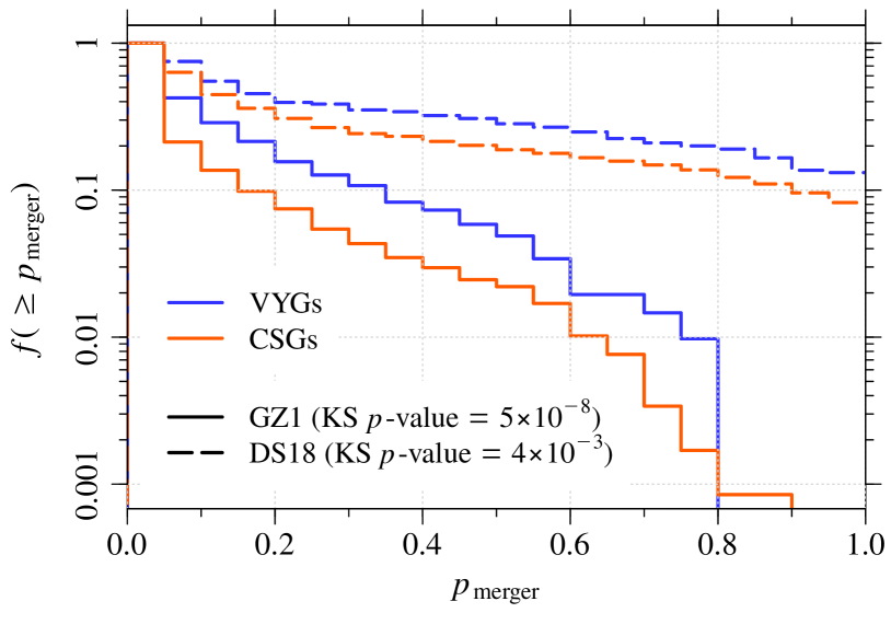
Figure 15: Fraction of galaxies that are classified as mergers in Galaxy Zoo (GZ1, solid lines) and by Domínguez Sánchez et al. (2018) (DS18, dashed lines) for different threshold values of $p_{\rm merger}$. The blue and orange lines correspond to the VYGs and CSGs, respectively.

Therefore, we performed our own visual classification based on the presence of tidal features indicating interactions with neighbour galaxies. The classification was performed independently by five members of our team. Each participant classified 414 galaxies (207 VYGs and 207 CSGs for comparison), and was asked to identify tidal features and signs of interactions in the test galaxies as well as their neighbours. To classify the galaxies, each vote received a value $v$, depending on how visible the interaction features are. The participants could answer yes, if they clearly see interaction signs ($v_{\tt yes}=1$), maybe if they are not sure ($v_{\tt mb}=0.5$) or no if they see none ($v_{\tt no}=0$). For the neighbours, the vote for no neighbours received $v_{0}=-1$. We then computed the mean of the values for the galaxy, $p_{\rm i,g}$, and its neighbour, $p_{\rm i,n}$, as follows:

$$p_{\rm i,g} \!\!\!\!=\!\!\!\! \frac{v_{\rm yes}\,N_{\tt yes,g}+v_{\tt mb}\,N_{\tt mb,g}}{N_{\rm votes}}\ ,$$

$$p_{\rm i,n} \!\!\!\!=\!\!\!\! \frac{v_{\rm yes}\,N_{\tt yes,n}+v_{\tt mb}\,N_{\tt mb,n}+v_{\rm 0}\,N_{\rm 0,n}}{N_{\rm votes}}\ ,$$

where $N_{\tt yes,g}$ and $N_{\tt mb,g}$ are the number of yes and maybe votes for the galaxy and $N_{\tt yes,n}$, $N_{\tt mb,n}$ and $N_{\rm 0,n}$ are the number of yes, maybe and no-neighbour votes for the galaxy neighbour. If the mean of the votes is $p_{\rm i}\geq 0.75$, the galaxy is classified as “interacting”. More details of our interaction classification scheme are given in Appendix B.

The advantage of our classification scheme of interactions is that it also considers the neighbouring galaxies. In Table 1, we compare the fractions of interacting VYGs and CSGs regardless of whether there is a neighbour, and also those of galaxies that have neighbours classified as interacting. We also computed the fractions of interacting galaxies that have no neighbour or those that have neighbours with no sign of interaction. In all three cases, the fraction of VYGs classified as interacting is roughly twice that of CSGs, in agreement with the results obtained with the Galaxy Zoo classification.

In Fig. 16, we show how the fractions of galaxies, classified as interacting according to our scheme, vary as a function of galaxy stellar mass. In the upper panel, we show the fractions of all interacting galaxies regardless whether there is a neighbour or not. The fraction of VYGs that are interacting is roughly independent of stellar mass at $\sim 30-40\%$, while the corresponding fractions of CSGs increases with $M_{\star}$ up to $M_{\star}\sim 10^{10}\,$M_⊙, and decreases again for $M_{\star}\mathrel{\hbox{\hbox to0.0pt{\hbox{\lower 4.0pt\hbox{$\sim$}}\hss}\hbox{$>$}}}10^{10}\,$M_⊙. The difference between these two samples is larger for low-mass galaxies: $38.8\%$ of the VYGs with $M_{\odot}<10^{9}\,$M_⊙ are classified as interacting, a fraction that is $8.5$ times higher than that of CSGs in the same mass range ($f_{\rm interacting}=4.5\%$).

The fraction of interacting galaxies with a companion also classified as interacting is shown in the lower panel of Fig. 16. For the VYG sample, $f_{\rm interacting}=6.1\%$ for galaxies with $M_{\odot}<10^{9}\,$M_⊙ and varies between $10$ and $15\%$ for more massive objects ($M_{\odot}>10^{9}\,$M_⊙). These fractions are $>6.7$ times higher when compared to those of the CSGs, except for the mass bin $9.5<\log(M_{\star}/{\rm M}_{\odot})<10$, where the $f_{\rm interacting}$ are similar for the two samples.

Could this higher fraction of interacting galaxies among VYGs be due to a surface brightness effect? The VYGs have higher surface brightness compared to the CSGs, as shown in Fig. 7. This could naturally lead to higher fractions of galaxies classified as interacting, since it would be easier to identify structures and features in the galaxy images. To test this hypothesis, we compared $f_{\rm interacting}$ in bins of $\mu_{50}$. As we can see in Fig. 17a, the fraction of interacting VYGs is always higher than that of CSGs with similar $\mu_{50}$, with differences ranging from $1.5$ to $5.2$ times higher, except for the brightest $\mu_{50}$ bin. But the difference is within the errors and might be a result of poor statistics, since there are only 3 CSGs in this bin. We conclude that the higher fraction of interacting galaxies among VYGs is not caused by surface brightness effects.

Finally, in Fig. 17b, we show $f_{\rm interacting}$ when both the galaxy and its neighbour(s) show signs of interactions. For the faintest $\mu_{50}$ bin ($\mu_{50}>22$), no systems are classified as interacting. The CSG fractions are lower than those of the VYGs for galaxies with $20.5<\mu_{50}<22$, but they are similar for brighter objects ($\mu_{50}<20.5$). However, the interpretation of these results is not straightforward, since these fractions also depend on the surface brightness of the neighbours that can be fainter than that of our galaxies.

In summary, VYGs exhibit a significantly higher fraction of mergers and interactions than do CSGs.

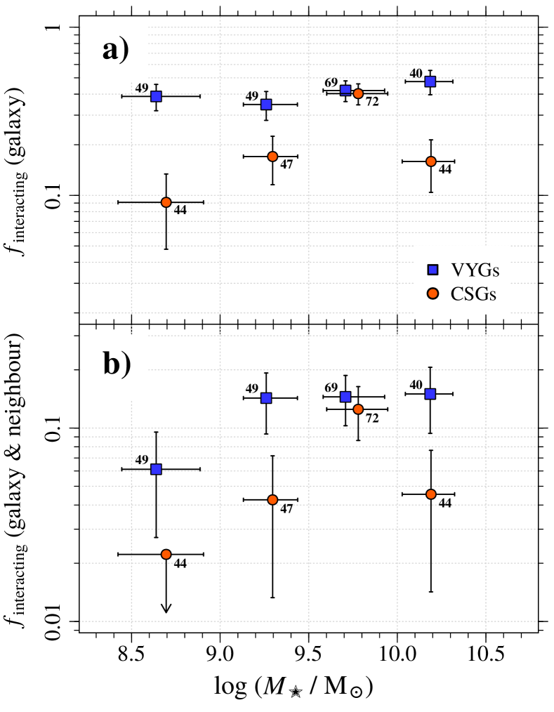
Figure 16: Fraction of galaxies with visually detected signs of interaction (from our 5-expert analysis) among VYGs (blue squares) and CSGs (orange circles), as a function of their stellar mass. In the upper panel, we include all galaxies classified as interacting, regardless of neighbours. In the bottom panel, we show the fractions of systems where the neighbour galaxy also show signs of interactions. The error bars indicate the $1\sigma$ binomial errors for $f_{\rm interacting}$ and the 16th and 84th percentiles of $\log M_{\star}$.

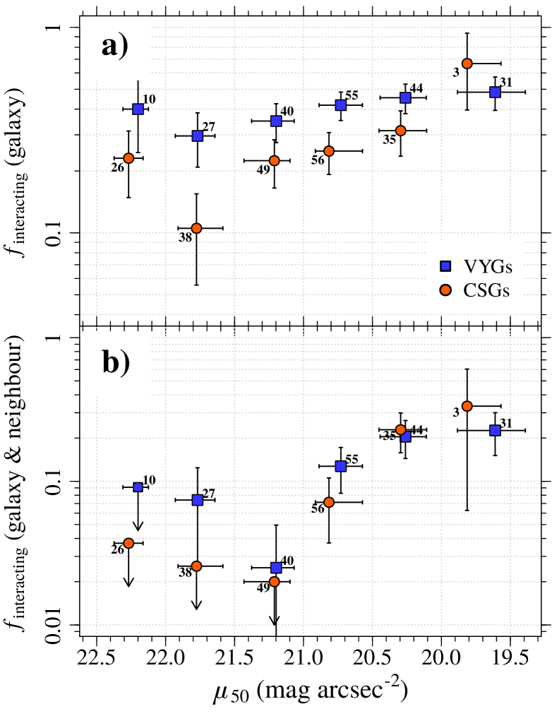
Figure 17: Fraction of VYGs (blue squares) and CSGs (orange circles) that show signs of interactions in bins of galaxy surface brightness. The notation is the same as in Fig. 16.

5.3 Group environment

We now analyze the group environment of the VYGs and CSGs. We selected groups and clusters from the updated version of the catalogue compiled by Yang et al. (2007). The catalogue contains $473\,482$ groups drawn from a sample of $601\,751$ galaxies, mostly from the SDSS-DR7 (Abazajian et al., 2009). Only groups with $\log(M_{\rm halo}/{\rm M}_{\odot})\geq 12.3$ were selected, and we assigned our sample galaxies to the nearest group, following the method described in Trevisan, Mamon & Stalder (2017b). A galaxy is assigned to the group that gravitationally attracts it the most, i.e. the group with the lowest distance, in units of virial radius, $r_{\rm vir}$.

We define $r_{\rm vir}$ of a group as the radius, $r_{100}$, of a sphere that is $\Delta_{\rm v}=100$ times denser than the critical density of the Universe. We obtained $r_{\rm vir}$ by first deducing $r_{200,{\rm m}}$ (of spheres that are 200 times denser than the mean density of the Universe from the $M_{200,{\rm m}}$ masses given in the Yang et al. catalogue (which are based on abundance matching with the group luminosities). We then calculated the $r_{\rm vir}$, following appendix A of Trevisan, Mamon & Khosroshahi (2017a) for the conversion from quantities relative to the mean density to those relative to the critical density, and the corresponding virial masses, $M_{\rm vir}=(\Delta_{\rm v}/2)\,H^{2}(z)\,r_{\rm vir}^{3}/G$.

To assign the galaxies to their nearest group, we compute the distances, $d$, between the galaxies and the group centres, assuming two regimes. For galaxies far away from the group, $d$ is given by the redshift-space distance. For a galaxy close to a group, the strong redshift distortions are taken into account by using the overdensity in projected phase space introduced by Yang et al. (2005, 2007). We convert this overdensity to an equivalent redshift-space distance by joining the two estimators at a given radius, $R_{\rm n}$, which marks the transition between the non-linear and the linear regimes. We adopt $R_{\rm n}=2\,r_{\rm vir}$, and galaxies can be assigned to distances up to $20\,r_{\rm vir}$ from a group. A small fraction ($<4\%$) of the galaxies was not assigned to any group (7 VYGs and 48 CSGs). Among these galaxies, 22 of them were not assigned because they lie at $z<0.01$, which is the lower redshift limit of the group catalogue. The other 33 galaxies lie close to the borders of the SDSS Survey or a bright star, and the group catalogue may be incomplete in these regions. Using the package MANGLE 2.1, as described in Sect. 5.1, we estimate that more than 20% of the region within $500\,$kpc from these galaxies lies outside the SDSS coverage area.

We computed the fractions of VYGs and CSGs at different distances from the group/cluster centre. Table 2 indicates that roughly half of galaxies are found at distances $R>3\,r_{\rm vir}$ from the group centres (52% and 58.4% of the VYGs and CSGs, respectively). Analysing the galaxies within groups, we see that VYGs reside preferentially in low-mass haloes compared to CSGs. As shown in Fig. 18 and Table 2, the fraction of VYGs that reside in groups with $\log(M_{\rm halo}/{\rm M}_{\odot})<13.5$ is $\sim$ 50 per cent higher than the corresponding fraction of CSGs. Fisher and Barnard tests indicate a high statistical significance for this result ($p$-values $=0.0006$ and $0.002$, respectively).

The way that the VYGs are distributed within and around the group haloes is also different from that of the CSGs. By comparison to CSGs, VYGs are more likely to lie within groups. As shown in Fig. 18 and Table 2, $~{}63\%$ of the CSGs in low-mass haloes are found between $1$ and $3\,r_{\rm vir}$, while only $43\%$ of the VYGs reside in this region. The fraction of VYGs that are centrals is double that of CSGs, with statistical tests indicating a marginal significance ($p$-values $\sim 0.02$).

Only a small fraction of VYGs and CSGs are in more massive haloes with $\log[M_{\rm halo}/{\rm M}_{\odot}]\geq 13.5$ ($12\%$ of the VYGs and $17.6\%$ of the control sample). But we find that VYGs are also more likely to be found in the inner parts of the these high-mass groups, with $54.2\%$ of the VYGs lying at distances $<1\,r_{\rm vir}$. For the CSGs, this fraction is only $32.4\%$, with statistical tests indicating that this difference is marginally significant ($p$-values $\sim 0.04$).

From the results shown in Fig. 18 and Table 2, we see that the VYGs are more likely to be found in the inner parts of low mass groups when compared to the CSGs. We find 41 VYGs that lie within $1\,r_{\rm vir}$ from the centre of low mass groups. These number corresponds to 20.5% of all 200 VYGs that were assigned to a halo. This fraction is much higher than that of CSGs residing in the inner regions of low-mass groups: only 9% (107 out of 1194) of the CSGs are at distances $<1\,r_{\rm vir}$ from the centre of haloes with $\log(M_{\rm halo}/{\rm M}_{\odot})<13.5$. Fisher’s and Barnard’s tests indicate high statistical significance, with $p$-values of $6\times 10^{-6}$ and $6\times 10^{-5}$, respectively.

We checked if the definition of the group and cluster centres could affect our results. In our group assignment scheme, we assume the position of the brightest group galaxy to be the centre of the group. Since VYGs have young stellar populations, they are expected to be brighter than non-VYGs with similar masses, and this could lead to higher fractions of VYGs that are centrals compared to normal galaxies. Therefore, we repeated our assignment procedure using the most massive galaxy as the centre of the group haloes. We find that the number of VYGs that are central galaxies in haloes with $\log(M_{\rm halo}/{\rm M}_{\odot})<13.5$ remains unchanged (17 VYGs). On the other hand, the number of centrals in the control sample decreases from 33 ($11.5\%$) to 27 ($9.2\%$), and the statistical significance of the result of a larger fraction of centrals in VYGs increases ($p$-values$=0.002-0.003$).

Table 2: Kolmogorov-Smirnov $p$-values for different comparisons between VYGs and CSGs

	$12.3\leq\log M_{\rm halo}<13.5$				$13.5\leq\log M_{\rm halo}$			Field	Total
	Centrals	$0-0.5\,r_{\rm vir}$	$0.5-1\,r_{\rm vir}$	$1-3\,r_{\rm vir}$	$0-0.5\,r_{\rm vir}$	$0.5-1\,r_{\rm vir}$	$1-3\,r_{\rm vir}$	$>3\,r_{\rm vir}$
VYGs	17 (23.6%)	14 (19.4%)	10 (13.9%)	31 (43.1%)	6 (25%)	7 (29.2%)	11 (45.8%)
	72 (36%)				24 (12%)			104 (52%)	200
Control	33 (11.5%)	38 (13.2%)	36 (12.5%)	180 (62.7%)	35 (16.7%)	33 (15.7%)	142 (67.6%)
	287 (24%)				210 (17.6%)			697 (58.4%)	1194
Fisher’s tests
$p$-value	0.013	0.192	0.843	0.003	0.392	0.146	0.042
	0.0006				0.052			0.104
Barnard’s tests
$p$-value	0.017	0.108	0.535	0.005	0.213	0.095	0.044
	0.002				0.065			0.065

Notes: The number of galaxies in groups are divided in bins of projected distance to the group centre, $R$. The number of central galaxies is shown only for low-mass groups, since none of our VYG and CSGs are found in the centre of high-mass groups. The last lines show the $p$-values of Fisher’s and Barnard’s tests comparing the fractions of VYGs and CSGs in each bin of $R$ and in the field. Results with $p$-values$<0.05$ are highlighted in boldface.

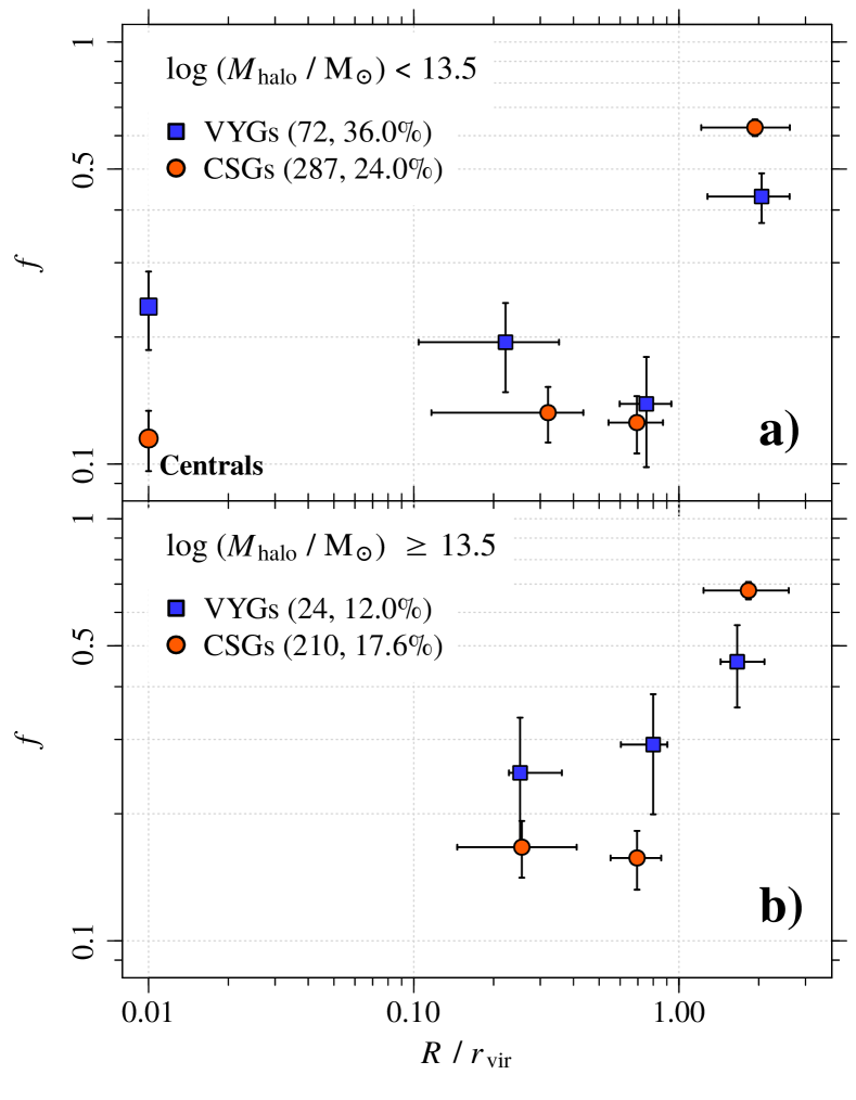
Figure 18: Distribution of radial positions relative to nearest group among VYGs (blue squares) and CSGs (orange circles). The upper and lower panels show the radial distributions of galaxies relative to low and high mass groups, respectively (there are no centrals among VYGs and CSGs in the higher mass groups, because nearly all centrals of high-mass groups are passive galaxies). The error bars indicate the $1\sigma$ binomial errors for $f$ and the 16th and 84th percentiles of $R/r_{\rm vir}$.

5.4 Large-scale environment: filaments and voids

The positions of our galaxies with respect to the large-scale filamentary structure were obtained from the catalogue of filaments established by Tempel et al. (2014). For each SDSS-DR7 galaxy, the catalogue provides the distance to the closest filament, $D_{\rm fil}$. Since the catalogue is based on SDSS-DR7 (while our samples were drawn from SDSS-DR12) and contains only galaxies in the main survey area ($6.5\mathrel{\hbox{\hbox to0.0pt{\hbox{\lower 4.0pt\hbox{$\sim$}}\hss}\hbox{$<$}}}{\rm RA}\mathrel{\hbox{\hbox to0.0pt{\hbox{\lower 4.0pt\hbox{$\sim$}}\hss}\hbox{$<$}}}18\,$h), $D_{\rm fil}$ is available for only 185 VYGs and 1126 CSGs.

There is no statistical difference between the VYG and CSG distributions of distances to the nearest filament (KS test $p$-value is$\,=0.22$), and similar fractions of VYGs and CSGs are within $D_{\rm fil}\leq D_{\rm max}=1\,$Mpc: $35.7\%$ of the VYGs and $31.6\%$ of the CSGs ($p$-values$\,=0.27$ and $0.31$ for Fisher’s and Barnard’s tests). In addition, the luminosities of the filaments containing VYGs and CSGs within 1 Mpc are similar. We used the luminosities $L_{0.5}$ and $L_{1.0}$ computed by Tempel et al. (2014) as the the sum of luminosities of observed galaxies that are closer than 0.5 and 1.0 $h^{-1}\,$Mpc from the filament axis. After removing the dependency of $L_{0.5}$ and $L_{1.0}$ on the stellar mass of the VYGs and CSGs, we see no significant differences between the distribution of luminosities of filaments containing VYGs and those containing CSGs (KS test $p$-values$\,=0.22$ and 0.08 for $L_{0.5}$ and $L_{1.0}$, respectively). Since an roughly half of VYGs and CSGs are within the virial spheres of groups, we investigated if the statistics of distance to nearest filaments are blurred by these galaxies. We repeated the analysis using only galaxies that are at distances $R>3r_{\rm vir}$ from all groups, and we still do not see any significant differences between the VYG and CSG distributions of $D_{\rm fil}$, $L_{0.5}$ and $L_{1.0}$.

We repeated the analysis using different maximum distances to the filaments ($D_{\rm max}=\,$0.2 up to 3 Mpc), but we find no significant evidence for higher (or lower) fractions of VYGs lying along the filaments compared to those of CSGs. The distributions of luminosities of filaments containing VYGs within $D_{\rm max}$ are also very similar to those of filaments containing CSGs, with KS tests indicating low statistical significance regardless of the $D_{\rm max}$ value adopted.

We also determined the position of our galaxies relative to voids by using the void catalogue by Sutter et al. (2012), which is also based on SDSS-DR7. To cover the redshift range of our sample, we also used three catalogues of voids that were identified using different samples of SDSS galaxies: dim1 (for galaxies at $0\leq z<0.05$), dim2 ($0.05\leq z<0.1$) and bright1 ($0.1\leq z<0.15$). We used the subcatalogues called “centrals” by Sutter et al. (2012). To avoid the biases introduced by the survey boundaries and masks, the centrals subcatalogues exclude voids that, when rotated in any direction about its barycentre, intersects a boundary galaxy.

For each VYG and CSG, we computed the distance to the centre of the closest void in units of the void radius, $D_{\rm void}$, assuming that the voids are spherical. The distances $D_{\rm void}$ are given by

$$D_{\rm void}=\frac{1}{r_{\rm void}\,(1+z_{\rm void})}\sqrt{\left[D_{\rm c}(z)-D_{\rm c}(z_{\rm void})\right]^{2}+\left[\theta\,\overline{D_{\rm c}}\right]^{2}}\ ,$$

where $z$ and $z_{\rm void}$ are the redshifts of the galaxy and the centre of the void, respectively; $\theta$ is the angular separation between the void centre and the galaxy; $D_{\rm c}(z)$ and $D_{\rm c}(z_{\rm void})$ are the comoving distances to the galaxy and to the void centre; $\overline{D_{\rm c}}$ is the mean comoving distance, $\overline{D_{\rm c}}=\left[D_{\rm c}(z)+D_{\rm c}(z_{\rm void})\right]/2$; and $r_{\rm void}$ is the void radius in Mpc. Since the catalogue is restricted to voids in the main survey area, we compute the distances for our galaxies within $6.5\mathrel{\hbox{\hbox to0.0pt{\hbox{\lower 4.0pt\hbox{$\sim$}}\hss}\hbox{$<$}}}{\rm RA}\mathrel{\hbox{\hbox to0.0pt{\hbox{\lower 4.0pt\hbox{$\sim$}}\hss}\hbox{$<$}}}18\,$h only (187 VYGs and 1155 CSGs).

Almost all of our galaxies (both VYGs and CSGs) are located far from the centre of the voids. Only $8.4\%$ of the galaxies (113 out of 1342) are at distances $D_{\rm void}\leq 1$, and the $p$-values of statistical tests do not provide any evidence that the VYGs prefer (or avoid) these low-density environments. We obtain $p$-values$\,=0.48$ and $0.67$ when applying Fisher’s and Barnard’s tests to the fractions of VYGs and CSGs that are at distances $D_{\rm void}\leq 1$ (18 VYGs and 95 CSGs, corresponding to $9.6\%$ and $8.2\%$, respectively). Both samples have similar $D_{\rm void}$ distributions, with median and standard deviations $D_{\rm void}=2.52\pm 1.38$ (VYGs) and $2.54\pm 1.27$ (CSGs). We applied a KS test to compare the distributions and obtained $p$-value$\,=0.22$. In summary, the large-scale environments of VYGs and CSGs are similar.

6 Discussion

6.1 How do very young galaxies differ from others?

Our comparison of the properties of VYGs and CSGs reveals that the VYGs are different from the general population of galaxies in many aspects. The results presented in Sections 3 to 5 can be summarized as follows:

• VYGs are bluer and have higher sSFRs than the CSGs. (Fig. 3), which confirms that our sample of VYGs indeed have younger stellar populations.

• In VYGs, the gas has higher ionization ratios (Fig. 4), which might be simply a consequence of higher sSFRs.

• VYGs contain a higher fraction of spheroidal systems compared to CSGs (Figs. 5 and 6). These VYG spheroids correspond to $\sim 6\%$ of sample and they are bluer than the CSG spheroids. On the other hand, we did not find significant differences between the overall distributions of VYG and CSG T-types, but most of our galaxies appear to be irregulars, so these catalogues may not provide a good description of their morphologies.

• VYGs have higher concentrations and surface brightness. (Fig. 7), indicating that the SF activity in VYGs is occurring in the inner parts of the galaxy. However, we cannot determine how the size of the VYGs compares to the general population of galaxies, since our control sample was defined by using the redshifts and angular effective radii in the PSM procedure; therefore, the VYG and CSG distributions of physical radii are similar by construction.

• VYGs are more asymmetric and more clumpy than CSGs. (Fig. 8), which may be a consequence of interactions with neighbour galaxies.

• Among galaxies detected in H i, VYGs have significantly higher fractions of atomic gas than CSGs (Fig. 10). Around $80\%$ of the VYGs with H i detections have $f_{\rm gas}>0.8$, while only $42\%$ of the CSGs have such high amounts of H i gas.

• The internal extinction in VYGs is higher than in the CSGs (Fig. 12), indicating that these young systems have a higher amount of dust compared to the general population of star-forming galaxies. We discuss the VYG internal extinction and dust content in Sect. 6.6.1.

• Compared to the CSGs, the VYGs are at smaller distances from their nearest companions and are more likely to be interacting/merging with a neighbour galaxy. These results are shown in Figs. 14 to 17 and Table 1, and will be discussed in Sect. 6.6.

• Roughly half of the VYGs lie outside groups; but compared to CSG, VYGs are more likely to be found in the inner parts of low-mass groups (Fig. 18 and Table 2). We discuss this result in Sect. 6.6.

Our sample of VYGs includes some starburst galaxies with very large H$\alpha$ equivalent widths, which are expected to have different properties. So, one could argue that the differences that we find between the VYG and control samples could be due to these objects. However, even when excluding these galaxies from our sample, the differences between the VYGs and the CSGs are still statistically significant, as indicated by the $p$-values in columns 3 and 4 of Table 3.

Although VYGs differ from the general population of galaxies in all the properties listed above, the VYGs are very similar to the CSGs in the following aspects:

• VYGs have the same gas metallicity as the CSGs (Fig. 9), except for hints of lower gas metallicity of VYGs at the low-mass end. We discuss in Sect. 6.2 the implications of the lack of differences in the gas metallicities of VYGs vs. CSG.

• The distribution of VYGs relative to cosmic filaments and voids is very similar to that of CSGs.

6.2 The VYG metallicities and relation with other young galaxies in the local Universe

The similar gas metallicities of VYGs and CSGs suggests that SF in VYGs is not being fuelled by infalling metal-poor gas, but by gas that was already enriched by previous generations of stars. This result has a consequence when comparing the VYGs with other populations of very young galaxies. As already discussed in Sect. 1, a few low-mass star-forming galaxies with extremely low metallicities in the local Universe, such as the blue compact dwarf galaxies I Zw 18 and SBS 0335–052, are strong VYG candidates. As shown by Izotov et al. (2019), these objects strongly deviate from the oxygen abundance vs. $M_{\star}$ relation defined by the bulk of star-forming galaxies. Therefore, the normal metallicities of VYGs at given mass suggests that VYGs do not resemble objetcs like I Zw 18.

Although we find that the gas mass fractions of VYGs with Hi detections is very high, I Zw 18 has an even more extreme $f_{\rm gas}$ value. The Hi mass of I Zw 18 is 50 times higher than its stellar mass, and the total neutral gas mass fraction is $f_{\rm gas}=0.98$. The most gas-rich VYG in our ALFALFA sample has $f_{\rm gas}=0.97$, and only 3 out of 16 VYGs with Hi detection have $f_{\rm gas}\geq 0.95$. But the stellar mass of I Zw 18 is 40 times lower than the lowest masses of our VYG sample, so it is difficult to make a meaningful comparison between this galaxy and the VYGs.

Furthermore, while our VYGs tend to have close companions, I Zw 18 appears to be a very isolated system. Indeed, using the same approach described in Sect. 5.1 to investigate the local environment of our VYG sample, and assuming $m_{r,{\rm I\,Zw\,18}}=16.4$ as the extinction-corrected Petrosian magnitude in the $r$ band of I Zw 18, we find that there is no other galaxy brighter than $m_{r}=m_{r,{\rm I\,Zw\,18}}+1$ up to $200\,$kpc from I Zw 18. This suggests that interactions with nearby galaxies cannot be the mechanism triggering the burst of SF in I Zw 18, and other processes must be invoked to explain the SF activity in this galaxy. But one cannot rule out the possibility that I Zw 18 has very recently grown by gas infall and/or mergers, as evidenced by its irregular morphology and the complex kinematics of its atomic gas (van Zee et al., 1998).

In any event, it is difficult to compare this population of extremely metal-deficient dwarf galaxies to the VYGs studied here. First, while these dwarfs have stellar masses $\sim 10^{5.5}-10^{8.0}$ M_⊙ (Izotov et al., 2014; Izotov et al., 2019), our sample is restricted to more massive objects with $M_{\star}>10^{8}\,$M_⊙. Moreover, the techniques employed to study the stellar populations of nearby dwarfs are different from those used here. Our ages were determined through SPS analysis of the integrated galaxy spectra, while the age of objects like I Zw 18 are inferred from colour-magnitude diagrams of resolved stellar populations. In Paper II, we determined the age of I Zw 18 using the same method (with STARLIGHT using the Vazdekis et al., 2015 spectral model) and found that 100% of its stellar mass was formed in the last $100\,$Myr, so this galaxy easily meets the VYG classification.

Since these metal-poor dwarfs are very nearby objects, with distances $\mathrel{\hbox{\hbox to0.0pt{\hbox{\lower 4.0pt\hbox{$\sim$}}\hss}\hbox{$<$}}}20\,$Mpc, it is very difficult to investigate their global environment. Catalogues of groups and clusters are not reliable at very low redshifts due to uncertainties introduced by peculiar velocities of galaxies. In addition, images of close objects contain more spatial information than those of galaxies at higher redshifts. Hence, morphological classification and morphometry of these galaxies (e.g. with Morfometryka) depend on galaxy distance, and correcting for this dependence to compare I Zw 18 analogues with our VYGs is beyond the scope of this paper.

Table 3: $p$-values of KS tests applied to the control and VYG samples

Property	KS $p$-values
	All	VYGs with	VYGs with
	VYGs	EW(H$\alpha$)$\,\leq 150\,$Å	EW(H$\alpha$)$\,\leq 100\,$Å
(1)	(2)	(3)	(4)
$\log{\rm sSFR}$	$<10^{-10}$	$9\times 10^{-10}$	$2\times 10^{-5}$
($g-i$)Petro	$5\times 10^{-4}$	$2\times 10^{-3}$	0.01
BPT diagram	$<10^{-10}$	$7\times 10^{-8}$	$3\times 10^{-5}$
$\log({\rm O/H})$	0.09	0.18	0.55
$f_{\rm gas}$	$2\times 10^{-4}$	$2\times 10^{-4}$	$7\times 10^{-5}$
$A_{V}^{\rm Balmer}$	$<10^{-10}$	$<10^{-10}$	$2\times 10^{-10}$
$A_{V}^{\rm cont}$	$9\times 10^{-7}$	$3\times 10^{-7}$	$3\times 10^{-8}$
$C_{1}$	$1\times 10^{-7}$	$3\times 10^{-6}$	$2\times 10^{-6}$
$\mu_{50}$	$<10^{-10}$	$<10^{-10}$	$6\times 10^{-8}$
$A_{1}$	$2\times 10^{-7}$	$3\times 10^{-5}$	$2\times 10^{-5}$
$S_{1}$	$3\times 10^{-3}$	0.02	$4\times 10^{-3}$
$d_{\rm 1st}/$kpc	$4\times 10^{-3}$	0.01	0.03
$d_{\rm 1st}/\theta_{50}$	$4\times 10^{-4}$	$5\times 10^{-3}$	0.03

6.3 VYGs versus late bloomer galaxies at intermediate redshifts

A sample of young systems at intermediate redshifts was recently studied by Dressler et al. (2018, hereafter DKA18). They derived the SFHs of galaxies at $0.45<z<0.75$ and with $M_{\star}>10^{10}\,$M_⊙, and identified a galaxy population of late bloomers (LB), i.e., galaxies that formed at least 50% of their stellar mass within 2 Gyr of the epoch of observations. Their SFHs were inferred from the Carnegie-Spitzer-IMACS Survey photometry.

DKA18 found that LBs account for $\sim 20\%$ of galaxies at $z\sim 0.6$, and their fractions systematically decrease with decreasing redshift, and the most massive LBs ($M_{\star}\mathrel{\hbox{\hbox to0.0pt{\hbox{\lower 4.0pt\hbox{$\sim$}}\hss}\hbox{$>$}}}10^{11}\,$M_⊙) pratically disappear at $z\sim 0$. In Paper II, we showed that the fractions of VYGs in the local Universe are consistent with the extrapolation of the fractions of LBs vs. redshift determined by DKA18 (see Fig. 14 in Paper II).

Are the properties of VYGs similar to those of LBs? It is difficult to answer this question, given the stellar mass ranges of the VYG and LB samples; while LBs are, by definition, more massive than $M_{\star}>10^{10}\,$M_⊙, most of our VYGs have $M_{\star}\mathrel{\hbox{\hbox to0.0pt{\hbox{\lower 4.0pt\hbox{$\sim$}}\hss}\hbox{$<$}}}10^{10}\,$M_⊙, and it is well known that galaxy properties correlate with stellar mass. A significant fraction of LBs appear to be spiral galaxies, but DKA18 also find some LBs with early-type morphology, with SEDs that are consistent with that of a post-starburst galaxy. Although VYGs appear to be mostly irregular, it is interesting that we also find an excess of spheroidal systems, suggesting that some common mechanism is producing young spheroidal systems at different redshifts.

One very interesting result obtained by DKA18 is that LBs avoid lying close to galaxies that are not LBs up to distances of $8\,$Mpc, indicating that galaxy SFHs can trace local and large-scale environmental histories. In Sect. 5.4, we found no difference between the VYG and CSG positions relative to filaments and voids, and the luminosities of the filaments close to VYGs and CSGs are also similar.

However, the distributions of VYGs and CSGs relative to the large-scale structures being similar does not mean that the properties of galaxies within these structures are also similar. To investigate this, we used the SDSS spectroscopic catalogue to identify the VYG and CSG nearest galaxies (in comoving units). As shown in Fig. 19, the nearest neighbours of VYGs tend to be younger compared to those that are close to CSGs, in agreement with DKA18. The difference is more pronounced for low-mass neighbours; VYG neighbours with $M_{\star}\leq 10^{10}\,$M_⊙ are $\sim 0.17\,$dex, on average, younger than CSG neighbours in the same stellar mass range ($p$-value$=0.02$). Since VYGs tend to have more close companions than CSGs, we checked if the neighbours in the immediate surroundings are leading to this result by comparing the ages of closest galaxies at distances $>1\,$Mpc only. We confirm that we see the effect in both small ($<1\,$Mpc, $p$-value$\,=0.02$) and large ($>1\,$Mpc, $p$-value$\,=0.04$) scales. This is also in agreement with DKA18, who found that LBs avoid non-LBs up to $\sim 8\,$Mpc, which means that the ages of the LB nearest galaxies are younger compared to the general population of galaxies.

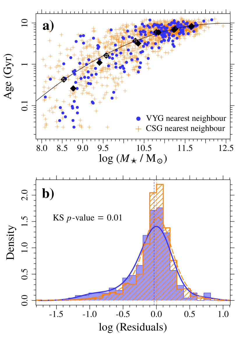
Figure 19: Top: Mass-weighted age of the VYG and CSG nearest SDSS spectroscopic galaxy (blue and orange symbols, respectively). The median ages in bins of stellar mass are indicated by the black diamonds, and the best-fit to the age-mass relation for the CSG neighbours is shown as the black solid line. Bottom: Distribution of the logarithm of the residuals from the best-fit relation shown in the top panel. The blue and orange histograms corresponds to the VYG and CSG nearest neighbours.

6.4 VYGs and CSGs in the low- and high-mass regimes

Table 4: Comparison of VYGs to control galaxies, splitting by mass

	$\log(M_{\star}/{\rm M}_{\odot})\leq 9.5$			$\log(M_{\star}/{\rm M}_{\odot})>9.5$
Property	VYG	KS $p$-value		VYG	KS $p$-value
	median			median
(1)	(2)	(3)		(4)	(5)
sSFR	higher	$<10^{-10}$		higher	$2\times 10^{-3}$
$(g-i)_{\rm Petro}$	lower	$1\times 10^{-9}$		same	0.10
BPT diagram	higher	$2\times 10^{-4}$		higher	$6\times 10^{-8}$
log(O/H)	lower	0.06		same	0.86
$f_{\rm gas}$	higher	$2\times 10^{-4}$		–	–
$A_{V}^{\rm Balmer}$	higher	$6\times 10^{-6}$		higher	$<10^{-10}$
$A_{V}^{\rm cont}$	lower	0.01		higher	$1\times 10^{-7}$
$C_{1}$	higher	$3\times 10^{-3}$		higher	$3\times 10^{-5}$
$\mu_{50}$	higher	$1\times 10^{-6}$		higher	$<10^{-10}$
$A_{1}$	higher	$4\times 10^{-5}$		higher	$3\times 10^{-3}$
$S_{1}$	higher	$0.08$		same	0.05
$d_{\rm 1st}/{\rm kpc}$	lower	0.06		lower	0.02
$d_{\rm 1st}/\theta_{50}$	lower	0.05		lower	0.01

Notes: For each property, columns 2 and 4 indicate how the median VYG value compares with that of the CSGs, while columns 3 and 5 show the respective $p$-values for that property in the corresponding mass bin. Changes in the trend between low and high mass are indicated in bold.

Our method of comparing the residuals to the CSG trend with mass of the properties of VYGs and CSGs may hide how differences between VYGs and CSGs vary from low to high stellar masses. To address this question, we repeated our analysis, separating the galaxies into two mass bins, above and below $\log(M_{\star}/{\rm M}_{\odot})=9.5$, which is close to the median of the VYG sample. Table 4 shows the results.

For several properties, we see similar trends for the VYGs compared to the CSGs in the low- and high-stellar mass regimes. On the other hand, differences between the VYG and CSG colours and asymmetries is seen only for low-mass galaxies. Furthermore, as already mentioned in Sect. 6.2, low-mass VYGs appear to be more metal-poor than CSGs with similar masses, and this is not observed for the high-mass VYGs. According to our merger diagnostics, merger events appear to be an important mechanism for VYGs of all masses, but the low gas metallicity in less massive VYG suggest both mergers and gas infall from the cosmic web are operating in the low-mass regime. This qualitatively agrees with our understanding that only high mass galaxies typically grow by mergers, which are too infrequent in low mass ones, which thus must usually grow by gas infall (Cattaneo et al., 2011). Following this argument, one would not expect that low-mass VYGs also have more neighbours, in contrast with the marginal indication of more neighbours around low-mass VYGs compared to low-mass CSGs shown in Table 4. Besides, all of the galaxies in our VYG and CSG samples have lower mass than the critical $z$ = 0 mass of $M_{\star}=2\times 10^{11}\,{\rm M_{\odot}}$ that Cattaneo et al. found for the growth by mergers (see Fig. 1). Nevertheless, one can reason that VYGs recently formed their stars by mergers, but will subsequently live a more quiet period of gas infall.

From low- to high-mass galaxies, we see a reversal of the trend of the VYG $A_{V}^{\rm cont}$ with respect to that of the CSGs, i.e., low-mass VYGs have lower $A_{V}^{\rm cont}$ values than the CSG values, while for high-mass VYGs we see the opposite. These high $A_{V}^{\rm cont}$ values might be responsible for the lack of bluer colours among high-mass VYGs. The behaviour of $A_{V}^{\rm cont}$ with galaxy mass, and the larger scatter that we observe in the $A_{V}^{\rm cont}-M_{\star}$ and $A_{V}^{\rm cont}-{\rm SFR}$ relations compared to the $\tau_{\alpha\beta}$ relations suggest that the amount of extinction of the stellar continuum might be determined by different – and maybe more – factors than the amount of extinction of the gas emission. We will further discuss the dust content in Sect. 6.6.1.

6.5 How can a galaxy retain so much gas for so long?

As shown in Fig. 10, among galaxies whose atomic gas is detected with ALFALFA, VYGs have very high atomic gas mass fractions, falling in the range 0.8–1, the same as found by Thuan et al. (2016) for extremely metal-deficient blue compact dwarf starburst galaxies. It is not clear if the ALFALFA sample is representative of the whole VYG population, but it seems that at least the low-mass VYGs with Hi detections have the amount of gas necessary to fuel the the intense SF activity required to form so many stars in such a small timescale. But how can a galaxy retain this gas until recent times?

A possible scenario comes from a recent study by Zhang et al. (2019), who, using data from SDSS, ALFALFA, GASS (Catinella et al., 2010) and COLD GASS (Saintonge et al., 2011), found that massive quiescent central disk galaxies contain as much atomic gas as corresponding star-forming galaxies ($M_{\rm HI}/M_{\star}>0.1$). Moreover, both galaxy classes have identical H i spectra indicating regularly rotating H i disks with radius $\sim 30\,$kpc and little kinematic perturbations. Following Renzini (2020), the H i gas in quenched disks can be stored in an outer ring with high angular momentum and large infall timescales. These galaxies are quenched because of the reduced molecular gas content and lower SF efficiency. However, perturbations could drive the outer atomic gas inwards and trigger SF.

This scenario could be extended to the lower masses of our VYGs. However, Zhang et al. only considered central galaxies, and only one out of the 17 VYGs that are centrals in low-mass groups ($12.3\leq\log[M_{\rm halo}/{\rm M}_{\odot}]<13.5$) has H i detection in the ALFALFA survey. All the other central VYGs are beyond the $z=0.05$ redshift limit of ALFALFA. We thus cannot determine if our central VYGs also have high fractions of atomic gas.

To investigate the gas fraction of low-mass central galaxies, we computed $f_{\rm gas}$ for a general sample of SDSS galaxies that have a counterpart in the ALFALFA catalogue. To avoid measurements of H i masses that may be contaminated by the neutral gas of nearby galaxies because of the large Arecibo beam size, we excluded galaxies that have companions within a radius of $1.8\,$arcmin and $\Delta z\leq 2\,W_{20}/c$, i.e., we adopt the same approach as described in Sect. 4.2. Fig. 20a shows $f_{\rm gas}$ vs. stellar mass of centrals and satellite galaxies in groups with $12.3\leq\log[M_{\rm halo}/{\rm M}_{\odot}]<13.5$, the same halo mass range of the central VYG haloes. We fitted the satellite $f_{\rm gas}$ vs. $\log M_{\star}$ relation assuming that $f_{\rm gas}$ can be described as

$$f_{\rm gas}=\frac{1}{1+\exp\,\left\{\sum_{i=0}^{4}\,a_{i}\,\left[\log(M_{\star}/{\rm M}_{\odot})\right]^{i}\right\}}$$

Fig. 20b shows the distributions of the residuals from the best-fit relation for the centrals and satellite galaxies with $M_{\star}<10^{11}{\rm M}_{\odot}$, which is the mass range of our VYG sample. Central galaxies tend to have higher fractions of atomic gas than satellites. This suggests that the higher gas fractions of VYGs may be related to their excess of centrals (Fig. 18).

Instead of retaining their gas, some VYGs may be experiencing gas infall from their surroundings. It could be pristine gas from the cosmic web, but, as already mentioned in Sect. 6.2, this only affects low-mass VYGs, at best, since high-mass VYGs have similar metallicities as CSGs of similar mass, while low-mass VYGs have a marginal indication of lower metallicity. Since a large fraction of the VYGs have companions, the VYG gas can be replenished by the gas from the merging neighbour galaxies. This is more likely than coming from the cosmic web of gas, since the gas brought in by the neighbouring galaxies is already somewhat enriched.

Although we find that VYGs appear to have more atomic gas, differences in the fraction of atomic (and molecular) gas alone cannot account for the observed distribution of objects above the main sequence of star-forming galaxies. Indeed, using data from the ALFALFA, GASS and COLD GASS surveys to quantify how the mean atomic and molecular gas mass fractions vary in the SFR-$M_{\star}$ plane, Saintonge et al. (2016) showed that galaxies with very high sSFR, such as those that are necessary to produce a VYG, not only have large gas fractions, but also have high SF efficiencies. It is known that mergers and interactions might enhance the efficiency in which the gas is converted into stars. We explore this scenario in the following Section.

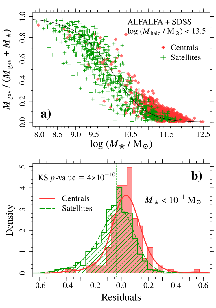
Figure 20: Top: Fraction of atomic gas in SDSS galaxies with H i detections in the ALFALFA survey as a function of galaxy stellar mass. The red and green symbols indicate the central and satellite galaxies in low-mass groups ($\log[M_{\rm halo}/{\rm M}_{\odot}]\leq 13.5$). The black solid line is the best-fit to the satellite $f_{\rm gas}$ vs. $\log M_{\star}$ relation (see text for details). Bottom: The residuals from the best-fit indicated in panel a for galaxies with $M_{\star}<10^{11}{\rm M}_{\odot}$. The red and green histograms correspond to low-mass centrals and satellites, respectively.

6.6 Are VYGs the products of mergers?

Many studies have shown that mergers and interactions induce an intense SF activity in galaxies (Joseph & Wright, 1985), with a recent exception (Pearson et al., 2019). Using hydrodynamical simulations, Di Matteo et al. (2008) found that the SF activity of starbursts triggered by mergers is enhanced by a factor of 3, on average, compared to starbursts in normal galaxies, and is greater than 5 in about 15% of major galaxy interactions and mergers. Moreover, multiple bursts can occur, with the bulk of SF among merging galaxies occurring at the 2nd passage, even though there is continuous SF, as well as a first burst at the first pericentre.

Our results suggest that mergers and interactions are important processes triggering recent SF activity. Compared to the control sample, the VYGs are twice as likely to have close companions at distances $<5\,\theta_{50}$ (Fig. 14). Moreover, the fraction of VYGs showing signs of interactions is double that of CSGs. Using the parameters $p_{\rm merger}$ from the DS18 and GZ1 catalogues, we have shown that the fraction of VYGs classified as mergers is always twice the corresponding fraction for CSGs, regardless of the threshold adopted for $p_{\rm merger}$ (Fig. 15). Our visual inspection of the SDSS images also shows that the fraction of VYGs showing sings of interaction is twice that of CSGs (Fig. 16 and Table 1), and this result does not depend on the galaxy surface brightness (Fig. 17).

The preference of VYGs to lie in the inner parts of low-mass groups (Fig. 18 and Table 2) also supports that scenario, since interactions and mergers are more likely to occur in this environment, where encounter velocities are slower, hence the encounters are more efficient (e.g., Mamon, 1992, 2000).

The VYG morphologies also point to the merging nature of a significant fraction of these systems, and may be related to different phases of mergers. VYGs are more clumpy and asymmetric than CSGs (Fig. 8), which may be signs of ongoing interactions with neighbour galaxies. In addition, VYGs have higher concentrations than CSGs (Fig. 7), indicating central SF activity. Hydrodynamical simulations show that global torques induced by mergers drive gas inwards, leading to more compact systems (Hopkins et al., 2010; Hopkins et al., 2013).

These compact galaxies are also seen as an excess of VYGs with low T-type values compared to those of the CSGs (Figs. 5 and 6). These early-type VYGs are bluer than CSGs with T-type$\,\leq 0$, and through a visual inspection of their images, we see that these systems are blue compact spheroids. These very compact VYGs could represent recent post-merger galaxies. Indeed, post-merger galaxies have 3 times higher gas fractions than control galaxies (Ellison et al., 2018). However, high gas fractions – as in our VYGs – reduce the loss of the gas angular momentum and increases the changes of disk survival (Hopkins et al., 2013). Therefore, the lack of disks in these galaxies suggests that the progenitor galaxies already had low angular momentum, such as irregular galaxies, or the orbital angular momentum of the merging system is low (i.e., head-on merging encounters). Otherwise, other mechanisms should be invoked to account for the formation of these blue compact VYGs.

6.6.1 Internal extinction, dust mass and relation with mergers

We found that VYGs have more internal extinction than CSGs, and this may be related to a merging process. As discussed in Sect. 4, at a fixed stellar mass, VYGs have higher $\tau_{\alpha\beta}$ (which probes the extinction in Hii regions) and $A_{V}^{\rm cont}$ (which is more related to dust in the diffuse ISM component) values compared to those of the CSGs (Fig. 12). While $A_{V}^{\rm cont}$ is inferred from the stellar continuum through SPS analysis, $\tau_{\alpha\beta}$ is obtained from H$\alpha$ and H$\beta$ emission lines. Since both parameters indicate that VYGs have higher internal extinction than CSGs, it is unlikely that this result is a consequence of biases and uncertainties in the SPS analysis or in the measurements of the emission line fluxes. Therefore, our results might be truly related to a higher amount of dust in VYGs compared to the general population of star-forming galaxies.

The high VYG $\tau_{\alpha\beta}$ values appear to be related to their high SFRs (Fig. 13a,b), since VYGs and CSGs follow a similar $\tau_{\alpha\beta}-\log{\rm SFR}$ relation. On the other hand, differences between the VYG and CSG $A_{V}^{\rm cont}$ do not appear to be fully accounted by differences in the galaxy sizes, morphology, inclination or SFRs. Differences between VYG and CSG gas metallicities cannot explain the higher amount of dust in VYGs either, since VYGs and CSGs have similar oxygen abundances (Fig. 9). Other factors can also contribute to higher internal extinction in VYGs, such as the HI gas mass (Casasola et al., 2020). However, the VYGs have higher $A_{V}^{\rm cont}$ and $\tau_{\alpha\beta}$ values compared to those of the CSGs at a fixed $f_{\rm gas}$. So, why do VYGs have more dust in their diffuse ISM component than CSGs? Ultra Luminous Infrared Galaxies (ULIRGs), whose very strong infrared emission is caused by dust, are observed to have one (Armus et al., 1987) or several (Borne et al., 2000) companions, implying that mergers triggered the extreme starburst leading to extreme amounts of dust.

Does the connection between star formation rates, dust and mergers extend to low-mass galaxies? To address this question, we analysed a sample of SDSS galaxies with very high SFRs and used the parameter $p_{\rm merg}$ from the catalogue of morphology by (Domínguez Sánchez et al., 2018; see Sect. 5.2) to access the probability of these systems of being mergers. A significant fraction of VYGs in our sample have $\log[{\rm SFR/(M_{\odot}\,yr}^{-1})]\geq 0.8$ (14.5%, i.e., 30 VYGs), and these galaxies are the ones associated with high internal extinction (see Fig. 13a). However, in a general sample of $\sim 323\,087$ SDSS galaxies at $z\leq 0.1$, only $4\,107$ ($\sim 1.3\%$) have these extreme SFR values, and they are typically more massive than $10^{10}\,$M_⊙. We analysed the internal extinction and merger probabilities of these $4\,107$ with very high SFRs by comparing them to a sample of galaxies with similar stellar masses and $\log[{\rm SFR/(M_{\odot}\,yr}^{-1})]<0.8$.

As expected, systems with high SFRs have larger $\tau_{\alpha\beta}$ and $A_{V}^{\rm cont}$ values compared to low-SFR galaxies with similar masses. In addition, we find that the distribution of $p_{\rm merg}$ is shifted towards higher values compared to those of the low-SFR galaxies, and the fraction of high-SFR galaxies with $p_{\rm merg}>0.5$ is almost two times larger than that of low-SFR objects ($26\%$ and $15\%$, respectively). The same results are observed when we consider only galaxies with $\log(M_{\star}/{\rm M}_{\odot})<10.5$; i.e., at lower stellar masses, galaxies with high SFRs also have more internal extinction and higher probabilities of being merging systems than low-SFR galaxies. Besides, in the low-mass regime, the differences between $p_{\rm merg}$ of high- and low-SFR galaxies is more pronounced when compared to the results obtained for all galaxies. The fraction of low-SFR systems with $p_{\rm merg}>0.5$ remains unchanged (15%), but this fraction increases to $42\%$ among the high-SFR low-mass galaxies. These results suggest that the relation between SFR, dust and merger events can be, at least at some level, extended to the low stellar mass regime, and the high SFRs and internal extinction that we find for our VYGs can be an indication of mergers and interations.

The internal extinction $\tau_{\alpha\beta}$ inferred from emission lines appear to be more related to the SFR and merger events than $A_{V}^{\rm cont}$. Once we take the $\tau_{\alpha\beta}$-SFR relation into account, we see no differences between the VYGs and CSGs. On the other hand, differences are still seen for $A_{V}^{\rm cont}$. Looking at Table 4, we see that the trend of VYG $A_{V}^{\rm cont}$ values compared to those of CSGs is reverted from low- to high-mass. Besides, the scatter in the $A_{V}^{\rm cont}-M_{\star}$ and $A_{V}^{\rm cont}-{\rm SFR}$ relations is larger compared to the relations for $\tau_{\alpha\beta}$. All these results suggest that dust production in the diffuse ISM is a complex process with several variables. While the properties of the molecular clouds in the star-forming regions of the galaxy appear to be dominant for $\tau_{\alpha\beta}$, $A_{V}^{\rm cont}$, tracing a more diffuse dust component, should depend on other galaxy properties, such as galaxy size, inclination, and the balance between the production and destruction of dust grains in the ISM. In other words, while the small-scale physics within molecular clouds appear to be roughly independent of the galaxy mass and properties, the processes regulating the production and destruction of dust in the ISM might more dependent of the galaxy integrated properties.

6.6.2 Predictions from models of galaxy formation

In Paper I (Tweed et al., 2018), we used analytical models of galaxy formation, which were applied to high-mass resolution Monte Carlo halo merger trees, to predict the fraction of VYGs in the local Universe. Four models were considered: one physically motivated model by Cattaneo et al. (2011), including a more realistic cut off at low halo masses due to reionization feedback (Gnedin, 2000, C+G); two empirical models by Moster, Naab & White (2013, MNW) and Behroozi, Wechsler & Conroy (2013, BWC), that use abundance matching to link the stellar-mass and the halo-mass functions; and an empirical model by Mutch, Croton & Poole (2013, MCP), where the stellar mass growth rate is proportional to the halo mass growth rate times a function of halo mass and redshift. The models were run with either the bursty or quiet halo merging schemes.

The effects of the bursty and quiet schemes on the predictions of VYG fractions depend on the model used. The merging scheme has virtually no effect on the VYG fractions versus stellar mass in the MNW and MCP models (fig. 10 of Tweed et al.). On the other hand, the VYG fractions in the quiet merging scheme are reduced by over one order of magnitude in the C+G model at intermediate mass and in the BWC model at low mass. Tweed et al. also showed that, with the bursty galaxy merging, VYGs are associated with a recent major halo merger, in contrast to the quiet merging scheme.

In Paper II (Mamon et al., 2020), we compared the predictions from these models to the observed fractions of VYGs. We found that the observations support the bursty scheme for C+G and BWC models, but little can be said about the bursty and quiet MNW and MCP models due to the small differences between these two schemes for these two models.

Since these models do not provide any prediction on the properties of the VYGs, no direct comparison between our results and these models is possible. However, we do present new constraints in favour of the bursty merging scheme, as our results indicate that, in comparison to CSGs, VYGs are more likely to be associated with gas-rich mergers.

6.6.3 Are most or all VYGs associated with mergers?

While we find many indications that mergers and interactions are responsible for triggering an intense SF activity in VYGs, it is not clear if these processes account for most or all of the VYGs. Our visual inspection of the VYG images revealed that at least half of our galaxies do not show any signs of interactions. However, the SDSS images are not deep enough, and we could be missing faint tidal features. So, future studies using deeper imaging data could help understanding the nature of those VYGs for which no signs of interactions are observed. In addition, since mergers leave signatures in the gas and stellar kinematics, spatially-resolved spectroscopic observations of VYGs might also help constraining this scenario, in particular to identify the isolated VYGs that are in a post-merger phase.

6.7 Caveats

6.7.1 Colour gradients and outer halo of old stellar populations

As described in Sect. 2.2, to minimize aperture effects due to the limited size of the SDSS fibre, we required that the total $g-i$ VYG colour be bluer than the corresponding fibre colour. We showed in Paper II that the requirement of a blue gradient does not rule out the possibility of a hidden old stellar population in the VYG, but at least it mitigates the aperture effect. But one must keep in mind that $i$) a blue gradient in a galaxy can also be a consequence of a negative metallicity gradient due to the age-metallicity degeneracy; and $ii$) this selection criteria can produce biased samples, as we discuss below.

It is known that different galaxy formation scenarios and physical mechanisms leave typical imprints on how the stellar population properties vary with the distance to the galaxy centre (Kobayashi, 2004; Hirschmann et al., 2015; Ferreras et al., 2019). Therefore, when imposing a blue gradient to select our galaxies, we favour physical mechanisms and formation scenarios that leave negative age and/or metallicity gradients. Several studies (e.g. Di Matteo et al., 2009; La Barbera et al., 2010, 2012; Bernardi et al., 2019; Zhuang et al., 2019; Zibetti et al., 2020) have shown that connecting observed galaxy gradients to the physical processes that produce them is not a straightforward task, so it is difficult to determine how this selection criteria affects our results and conclusions. Although the CSGs were selected to have negative (blue) colour gradients as for the VYGs, we cannot claim that our results and conclusions can be extended to VYGs that have positive (red) colour gradients.

6.7.2 Uncertainties in the spectral analysis

Young stellar populations are much more luminous than old ones. So, even within the fibre, the young population can outshine the old stars, making it hard to be detected through SPS analysis of the SDSS spectra and possibly leading to the overestimation of the fraction of mass in populations younger than 1 Gyr, $f_{M_{\star},{\rm y}}$.

To investigate the uncertainties in the determination of $f_{M_{\star},{\rm y}}$ using the STARLIGHT code, we used the Vazdekis et al. (2015) spectral models to create a set of simulated spectra assuming two bursts of SF, one occurring within the last 1 Gyr and the other 12 Gyr ago. The age of the young population was randomly selected among 21 ages between 0.03 and 1 Gyr, while the old population has a fixed age of 12 Gyr. We used as input $f^{\rm in}_{M_{\star},{\rm y}}=0.1,0.2,0.3$ and 0.4, and created 1000 simulated spectra for each $f^{\rm in}_{M_{\star},{\rm y}}$. The internal extinction and S/N of the simulated spectra were selected from the distributions of $A_{V}^{\rm cont}$ and S/N of the VYG sample.

Table 5: False positive VYGs from simulated spectra

$f^{\rm in}_{M_{\star},{\rm y}}$	median $f^{\rm out}_{M_{\star},{\rm y}}$	fraction of runs
		with $f^{\rm out}_{M_{\star},{\rm y}}\geq 0.5$
(1)	(2)	(3)
0.10	$0.10^{+0.04}_{-0.07}$	0.1%
0.20	$0.19^{+0.11}_{-0.12}$	6.9%
0.30	$0.31^{+0.38}_{-0.18}$	20.7%
0.40	$0.46^{+0.48}_{-0.29}$	44.0%

Notes: Columns are (1) Input mass fraction of the young stellar population (age $<1\,$Gyr); 1000 simulated spectra were created for each $f^{\rm in}_{M_{\star},{\rm y}}$ value. (2) Median of the output $f^{\rm out}_{M_{\star},{\rm y}}$ values; the upper and lower errors were obtained from the 84th and 16th percentiles of the $f^{\rm out}_{M_{\star},{\rm y}}$ distributions. (3) Fraction of runs with $f^{\rm out}_{M_{\star},{\rm y}}\geq 0.5$.

We ran STARLIGHT with the same configuration used in the SDSS spectral analysis of Paper II, and computed the fraction of runs with output $f^{\rm out}_{M_{\star},{\rm y}}\geq 0.5$, i.e., the fraction of simulated galaxies that would be wrongly classified as VYGs. We show the results in Table 5, where we also present the median of the $f^{\rm out}_{M_{\star},{\rm y}}$ values obtained.

We find a good agreement between the median estimated fraction of young mass and the input fraction. The fraction of incorrect VYG classifications rises very rapidly with the fraction of young stars: from rare with 10 per cent of young mass in the input spectra to 44 per cent with 40 per cent of young mass in the spectrum. This indicates that the reliability of the VYG classification is not too low.

It is difficult to estimate the number of false VYGs in our sample, because we do not know neither the true distribution of $f_{M_{\star},{\rm y}}$ nor the age and duration of the past and recent bursts of SF. Besides, our 2-burst simulations with are very simplistic. On the other hand, they represent a ‘worst’ possible scenario of a very old and low-luminosity population (12 Gyr) mixed with a very recent burst (< 1 Gyr). Many studies show that the SFHs of real low-mass galaxies are more extended (Thomas et al., 2010; De Lucia et al., 2006; Trevisan et al., 2012), and their old ($>\,1\,$Gyr) stellar component would be brighter and thus easier to detect than the population in our simulations, which was formed in single burst 12 Gyr ago. Nevertheless, we argued in Paper II that a conservative lower limit on the reliability of the VYG classification combined with the observed cosmic SFH implies that present-day galaxies with $M_{\star}>10^{8}\,$M_⊙ experienced, on average, at most four major starbursts over cosmic time.

In summary, our simulations show that it is possible that the fraction of mass in populations younger than 1 Gyr in some of our VYGs is, in fact, less than 50%. But our results suggest that, even if $f_{M_{\star},{\rm y}}$ is less than 50%, the young population still accounts for a significant fraction of the total stellar mass of the galaxy ($f_{M_{\star},{\rm y}}\mathrel{\hbox{\hbox to0.0pt{\hbox{\lower 4.0pt\hbox{$\sim$}}\hss}\hbox{$>$}}}30\%$). In addition, the results from 3 different spectral models have been combined to increase the reliability of our VYG sample.

Finally, one may think that the SPS analysis is not the proper method to derive the fraction of mass of young populations in galaxies, due to the large uncertainties associated with this method, in particular for galaxies with few absorption features in their spectra (such as galaxies with a very recent starburst). However, the differences in the properties of VYGs relative to our control sample confirms that these systems are different, i.e. younger. These differences cannot be attributed to the presence of starburst galaxies with large equivalent widths of H$\alpha$ in the VYG sample, since our conclusions remain unchanged when we exclude these galaxies from the VYG sample (see Table 3). Besides, we found differences in properties that were derived through methods that are independent of the SPS analysis, such as morphology, environment, the $\tau_{\rm\alpha\beta}$ measure of interstellar dust, and the gas mass fraction.

6.7.3 Imperfect control sample

As discussed in Sect. 2 and shown in Fig. 2a, the $\log M_{\star}$ vs. $z$ distribution of the CSGs is slightly different from that of the VYGs. To investigate if it affects our results, we repeated all the analysis presented in this work after excluding the galaxies that are more than $2\sigma$ away from the CSG $\log M_{\star}$ vs. $z$ relation (29 VYGs and 53 CSGs). We used a 2nd-order polynomial to fit the relation. All the results presented in Table 3 remain statistically significant with $p$-values below $<5\times 10^{-3}$, except for the parameters ($g-i$)_Petro, $S_{1}$, and $d_{\rm 1st}/$kpc, for which KS tests indicate marginal statistical significance with $p$-values$\,=0.04$, 0.01 and 0.03, respectively. Therefore, we conclude that the outliers in the $\log M_{\star}$ vs. $z$ relation do not affect our results and conclusions.

6.7.4 Nebular continuum emission

The SPS fitting of the spectra with STARLIGHT and VESPA both ignored the nebular contribution to the continuum, which becomes important in strongly star-forming galaxies. The ratio between the ionized gas and the continuum emissions increases with wavelength, ranging from $\sim 20\%$ at $\sim 4000\,$Å to more than $40\%$ around $7000\,$Å in galaxies with very high sSFRs (Izotov et al., 2011). As discussed in Paper II, the neglect of this red nebular component causes the SPS analysis to overestimate the ages of starburst galaxies. This was confirmed by Cardoso, Gomes & Papaderos (2019), who found that the FADO SPS code, which includes the nebular continuum emission in the fit, obtains lower ages than does STARLIGHT. Therefore, including the nebular continuum emission in our analysis would lead to even higher fractions of stellar mass formed within the last 1 Gyr, and would not affect the results and conclusions presented in this work.

7 Summary and Conclusions

In this work, we investigated the properties and environments of very young galaxies. The SFHs of galaxies were inferred from SDSS spectra through SPS analysis, and we selected as VYGs those galaxies with over half their stellar mass formed within the last $1\,$Gyr according to each of three different stellar population models. We built a control sample of normal galaxies with similar stellar masses, redshifts, radii and colour gradients, and the comparison between these two samples revealed that VYGs have different properties and reside in different environments. In Sect. 6.1, we summarise all the VYGs properties that we investigated and discuss how they compare to those of CSGs. From our results, we conclude that:

• VYGs and other young systems like I Zw 18 are likely to be different in nature, as discussed in Sect. 6.5. I Zw 18 analogues are low-mass very metal-poor systems that deviate from the mass-metallicity relation of normal galaxies, while VYGs follow it.
  

• Star formation in the more massive VYGs is not being fed by infalling metal-poor gas from the cosmic web, since these galaxies have similar gas oxygen abundances as the control galaxies. But gas infall and mergers may both be important triggers of star formation in the VYGs at the low-mass end, given hints of their lower metallicities and their excess of near neighbours.
  

• Gas-rich mergers and interactions are important mechanisms for producing very young systems in the local Universe (Sect. 6.6). Differences in the morphology (VYGs are more clumpy, more asymmetric and a larger fraction show tidal features and other signs of interactions compared to the CSGs) and the environment (VYGs are more likely to have companions and to be found in the inner parts of low-mass groups) of the VYGs support this scenario, in particular for the massive VYGs. These results agree with the predictions by Tweed et al. (2018, Paper I) for their subset of analytical models of galaxy formation where halo mergers are associated with starbursts.

Since mergers leave typical signatures in the gas and stellar kinematics of the galaxy, future studies of VYGs using spatially-resolved spectroscopic data can help constraining the merger scenario. Moreover, deep imaging data might help understanding the nature of the VYGs for which there is no evident sign of interactions in the SDSS images. We have also obtained GMRT and VLA HI radio observations to investigate the gas distribution and kinematics in and around VYGs.

Finally, in the present study, we showed that the VYGs differ from normal galaxies in various ways, but did their progenitors have peculiar properties before becoming VYGs? Or does any galaxy can become a VYG? In a future study, we will address the nature of the VYG progenitors by identifying these systems in hydrodynamical simulations and tracing back the assembly history of these systems.

We provide an electronic table with observed and derived properties of our VYGs and CSGs. The description of the table columns are given in appendix C.

Data availability

The data underlying this article are available in the article and in its online supplementary material.

Appendix A Determination of the Red Sequence at different redshifts

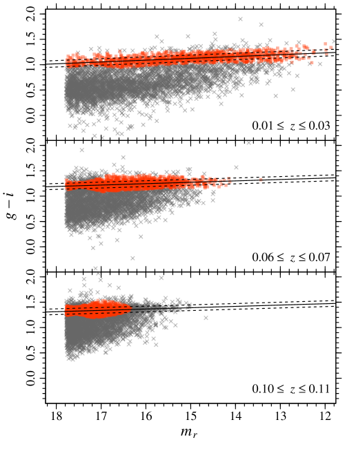
Figure 21: Identification of Red Sequence galaxies in the colour-magnitude diagram for three different bins of redshifts, using mclust (see text).

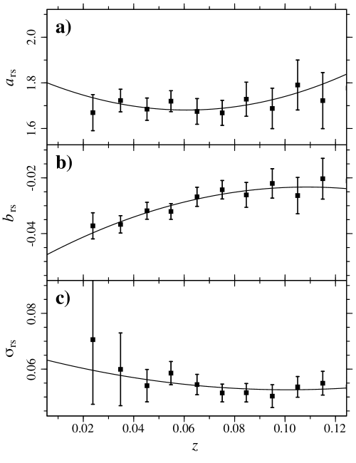
Figure 22: Parameters of the fit to the Red Sequence galaxies at different redshifts, where $(g-i)(m_{r},z)=a_{\rm RS}(z)+b_{\rm RS}(z)\,m_{r}$ with scatter $\sigma_{\rm RS}(z)$.

As described in Sect. 5, we relied on the photometric SDSS data to identify neighbouring galaxies and determine the local environment of our galaxies. This approach allows the identification of companions that are fainter than the MGS flux limit of $m_{r}=17.77$, which is the magnitude limit below which the spectroscopic catalogue is 95% complete. This also avoids the spectroscopic incompleteness due to the SDSS fiber collision issue. However, by using the photometry only, our determinations of the local environment will be affected by projection effects. Therefore, we used the spectroscopic catalogue to identify the Red Sequence (RS) at different redshifts, and used these relations to mitigate the contamination by background galaxies by excluding objects that are $2\,\sigma$ above the Red Sequence.

We identified the position of the RS in the colour-magnitude diagram at different redshifts, as follows. We retrieved galaxies from the SDSS spectroscopic catalogue within $0.01\leq z\leq 0.2$, and divided the sample in 18 bins of redshift in steps of $\Delta z=0.01$ (except the first bin, which includes galaxies in the range $0.01\leq z<0.03$). For each bin, we identified the galaxies belonging to the RS using mclust (Fraley et al., 2012; Fraley & Raftery, 2002), which is an R package for model-based clustering, classification, and density estimation, based on Gaussian finite mixture modelling via expectation-maximization. We ran mclust on 100 bootstrap re-samplings for each redshift bin, selecting 5000 galaxies in each realization. Once the RS is identified, we then fit the $(g-i)_{\rm rs}=a_{\rm RS}+b_{\rm RS}\,m_{r}$ relation and its scatter, $\sigma_{\rm RS}$. Figure 21 illustrates the procedure showing three different redshift bins.

Fig. 22 shows how $a_{\rm RS}$, $b_{\rm RS}$, and $\sigma_{\rm RS}$ vary with $z$. We fitted these relations with a 2nd-order polynomial, weighting the data points by the inverse of the squared error, obtaining:

$$a_{\rm RS}(z) = 1.826-4.759\,z+39.054\,z^{2}\ ,$$

$$b_{\rm RS}(z) = -0.05024+0.49631\,z-2.28545\,z^{2}\ ,$$

$$\sigma_{\rm RS}(z) = 0.06452-0.23577\,z+1.16574\,z^{2}\ .$$ (2)

Appendix B Visual classification of interacting and merging galaxies

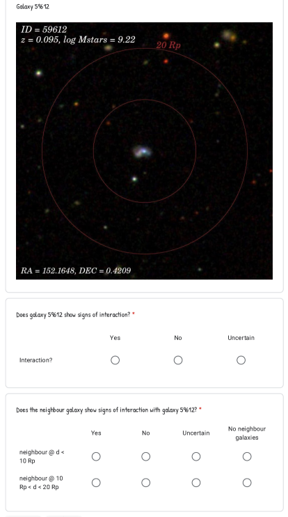
Figure 23: Example illustrating our form for visual classification of merging and interacting galaxies. This particular galaxy was classified as interacting system with both galaxy and neighbour showing signs of interaction.

We visually inspected our galaxies to identify features indicating interactions and recent mergers. While this approach is subjective, our eyes can still catch some features that the morphometry of galaxies is not able to. Besides the 207 VYGs, we selected 207 randomly chosen CSGs for comparison, and these 414 galaxies were classified by 5 participants, all astronomers.

We aimed to identify the following types of objects:

1.

Interacting / merging systems: the galaxy has one or several companions, at least one of which shows tidal features and/or other signs of interactions;

2.

Pairs / multiple systems: the galaxy has one or several close companions, but no clear sign of interaction between them (we might miss the tidal features because the SDSS images are not deep enough – or the pair is just a projection effect);

3.

Post-mergers: we see signs of recent interaction, i.e., tidal tails, but no neighbour galaxy;

4.

Non-interacting, isolated systems: no signs of interactions and no neighbour galaxies.

For this classification, we created a form with the galaxy images and the following questions, as shown in Fig. 23. The following instructions were given to the participants:

• Does the galaxy show signs of interaction, like tidal distortions and tails?

  If there are tidal features, the participants were instructed to answer yes to this question even if there are no neighbour galaxies, since we also want to identify post-mergers.

• Does the neighbour galaxy show signs of interaction with the test galaxy?

  This question is divided in two parts, one for neighbour galaxies within $10\,R_{\rm p}$, where $R_{\rm p}$ is the Petrosian radius in the $r$ band of our test galaxy, or for neighbour galaxies between $10$ and $20\,R_{\rm p}$. In each image, the $10-$ and $20-R_{\rm p}$ regions are indicated by red circles, as indicated in Fig. 23.

Appendix C VYG images and data

Figs. 24 to 27 show the SDSS images of the 207 VYGs analysed in this study. Each image displays the galaxy coordinates, redshift, and stellar masses derived with STARLIGHT using the Vazdekis et al. (2015) spectral models.

We provide the observed and derived properties of our VYGs and CSGs as supplementary data available online. The description of the table columns are given below.

(1) ObjID: SDSS objID

(2) specObjID: SDSS specObjID

(3) plate: SDSS spectroscopic plate

(4) mjd: SDSS modified Julian date of spectroscopic observation

(5) fiberID: SDSS spectroscopic fibre

(6) RA: right ascension (J2000)

(7) DEC: declination (J2000)

(8) z: galaxy spectroscopic redshift

(9) logMs_Vaz15: Present-day galaxy stellar mass obtained using the STARLIGHT code with Vazdekis et al. (2015) model

(10) C: galaxy concentration, defined as $\log(\theta_{90}/\theta_{50})$, where $\theta_{90}$ and $\theta_{50}$ are the radii containing 90% and 50% of the Petrosian flux in the $r$ band (SDSS parameters petroR90_r and petroR50_r)

(11) mu_50: galaxy surface brightness, computed using Eq. 1

(12) logA1: decimal logarithm of the asymmetry parameter, computed using the code Morfometryka

(13) logS1: decimal logarithm of the smoothness parameter, computed using the code Morfometryka

(14) logOH: gas oxygen abundance $\log({\rm O/H})+12$

(15) f_gas: gas mass fraction

(16) Av_Balmer: internal extinction in the $V$ band estimated from the Balmer decrement

(17) Av_cont: internal extinction in the $V$ band estimated from the SPS analysis using STARLIGHT with Vazdekis et al. (2015) models

(18) d_1st_kpc: distance, in kpc, to the closest neighbour galaxy brighter than $m_{r}+1$, where $m_{r}$ is the $r$-band Petrosian magnitude of our galaxy

(19) d_1st_norm: distance, in units of $\theta_{50}$, to the closest neighbour galaxy brighter than $m_{r}+1$, where $m_{r}$ is the $r$-band Petrosian magnitude of our galaxy

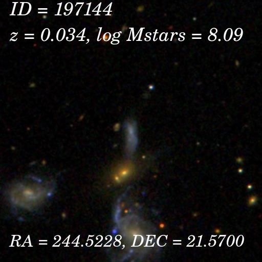
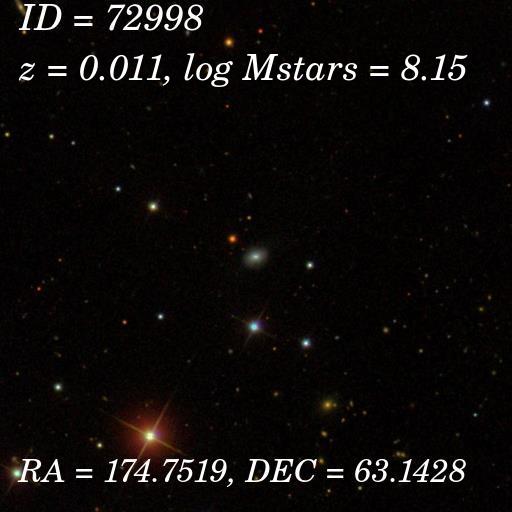
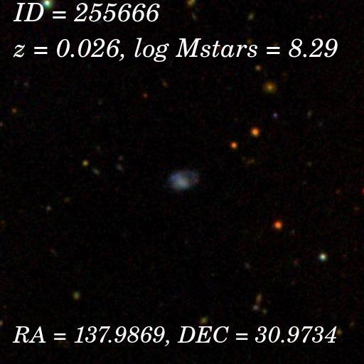
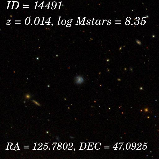
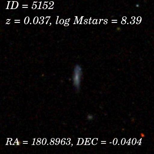
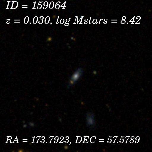
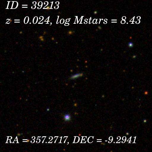
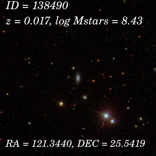
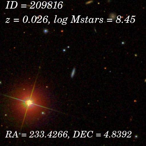
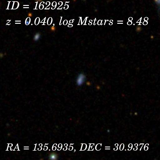
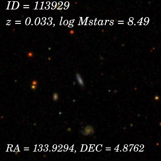
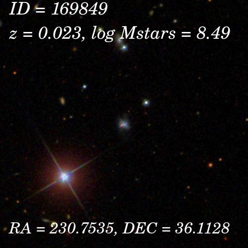
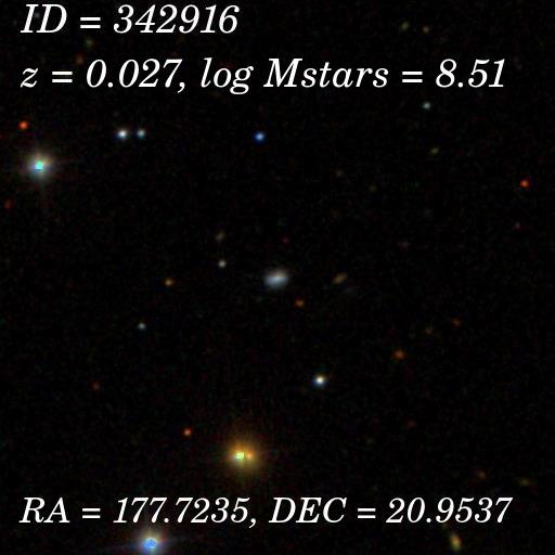
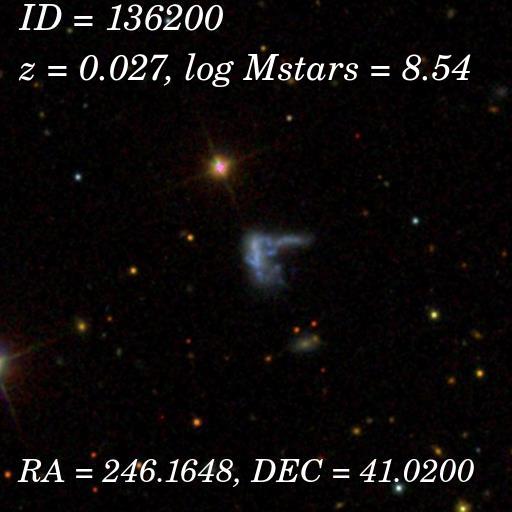
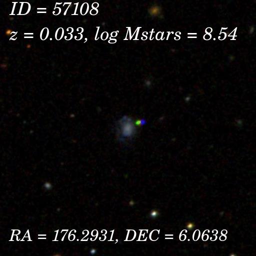
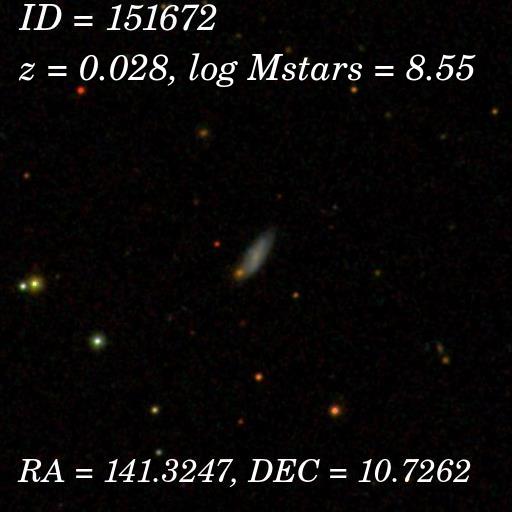
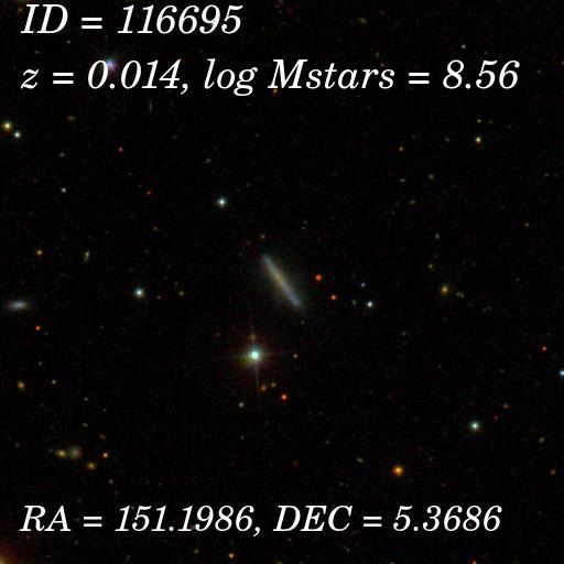
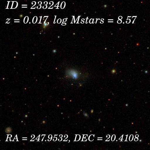
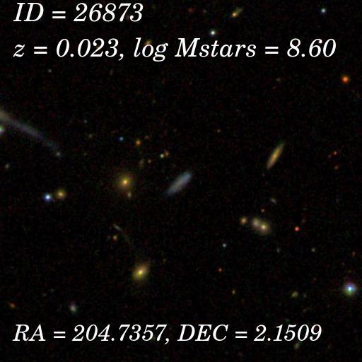
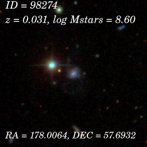
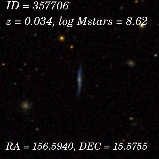
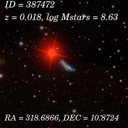
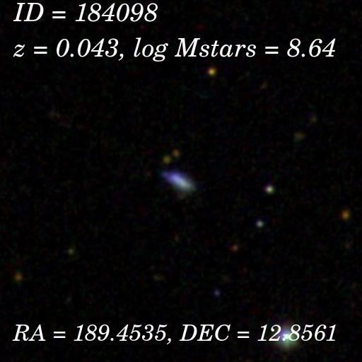
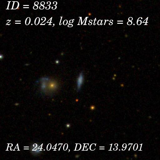
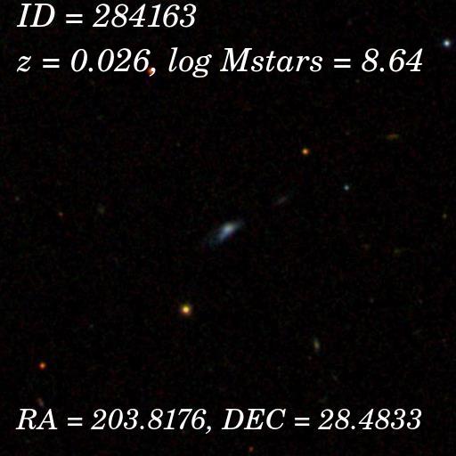
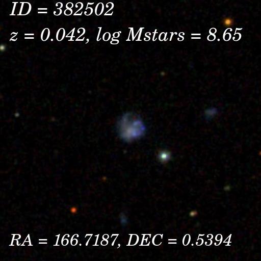
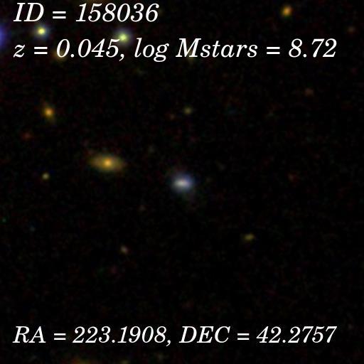
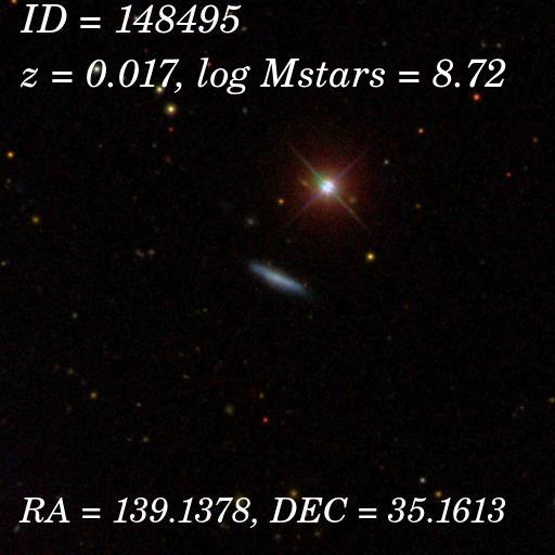
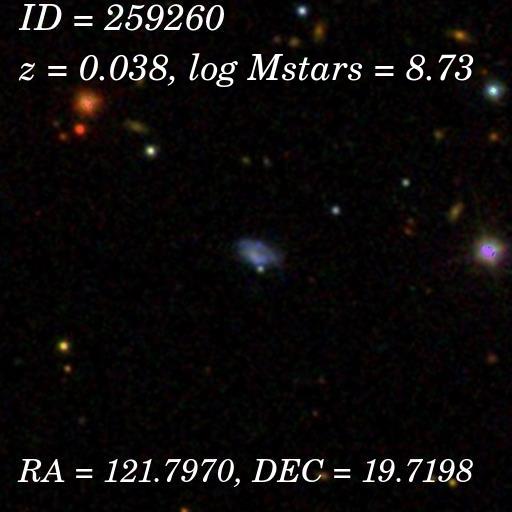
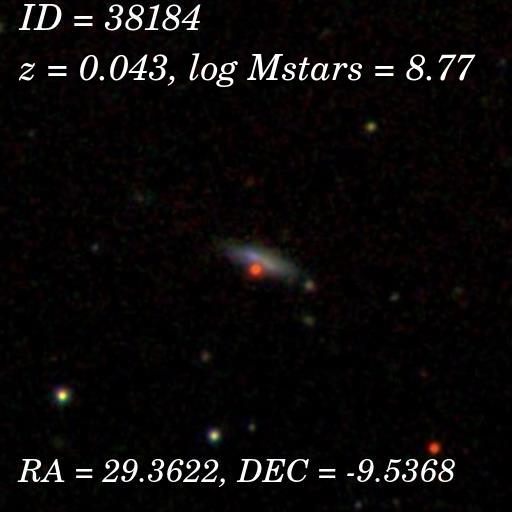
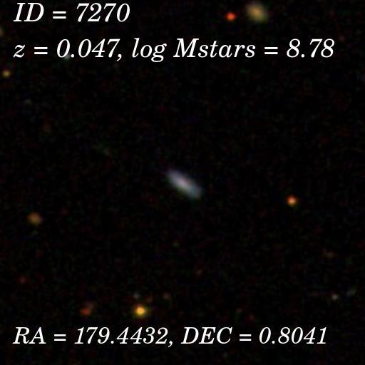
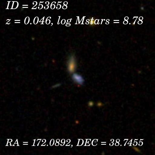
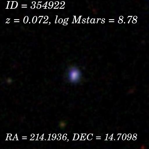
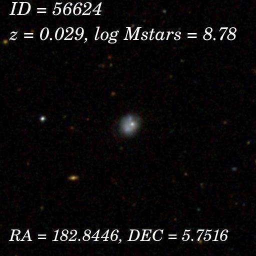
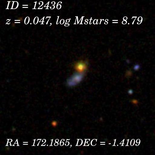
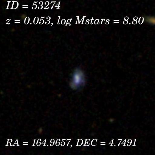
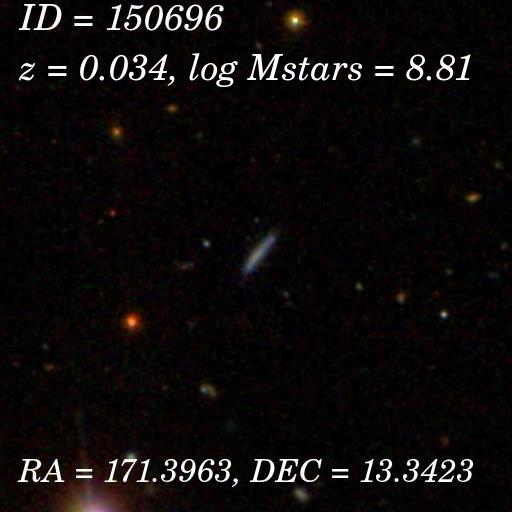
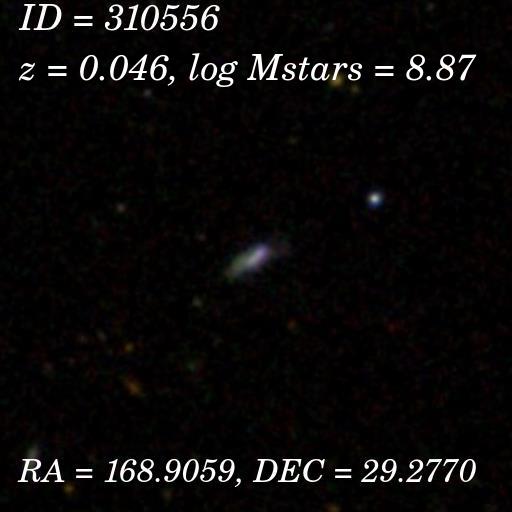
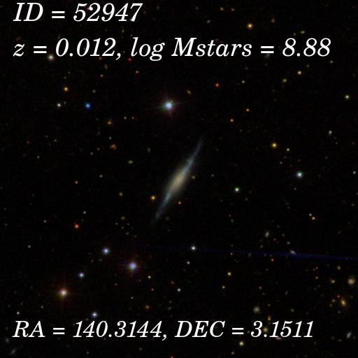
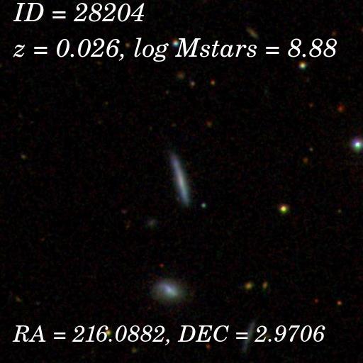
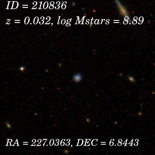
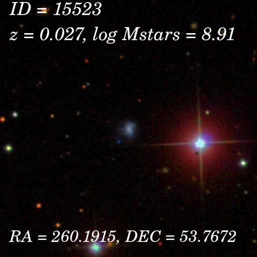
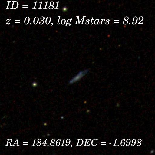
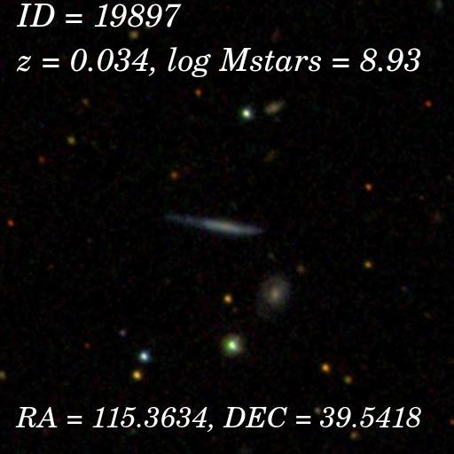
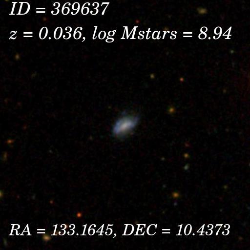
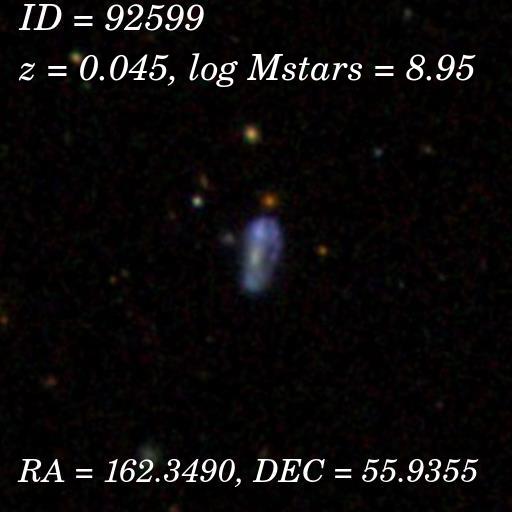
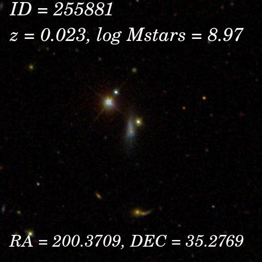
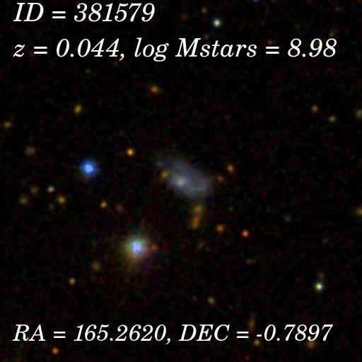
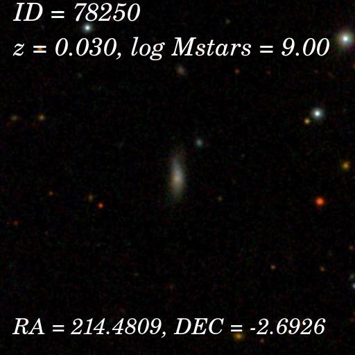
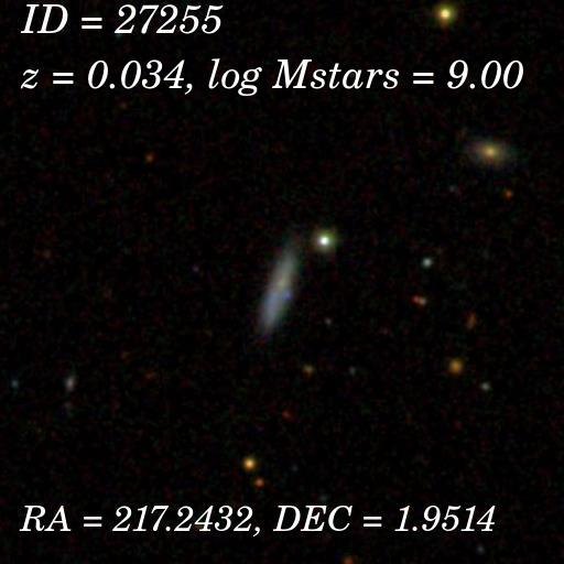
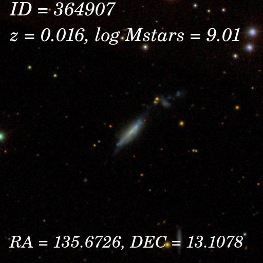
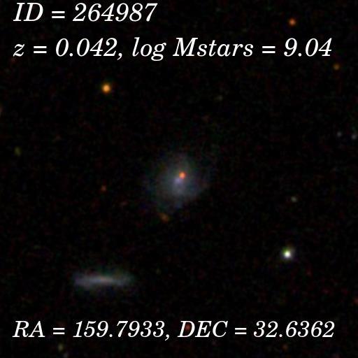
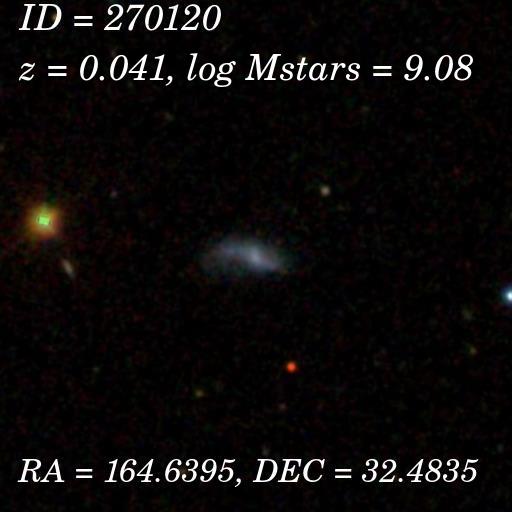
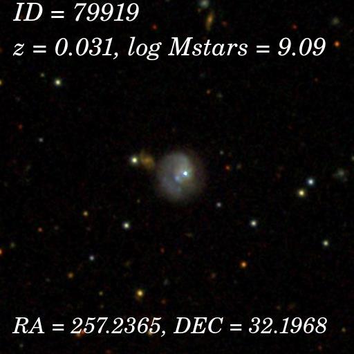
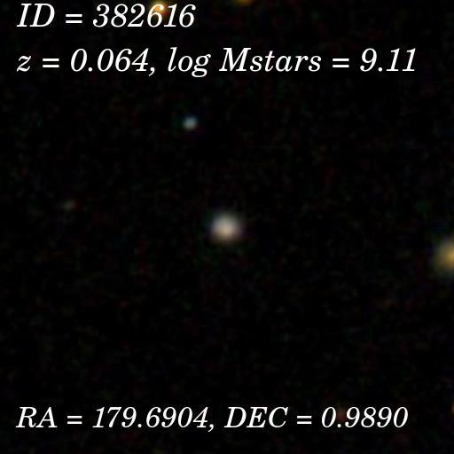
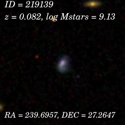
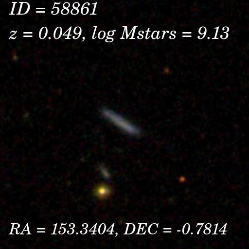
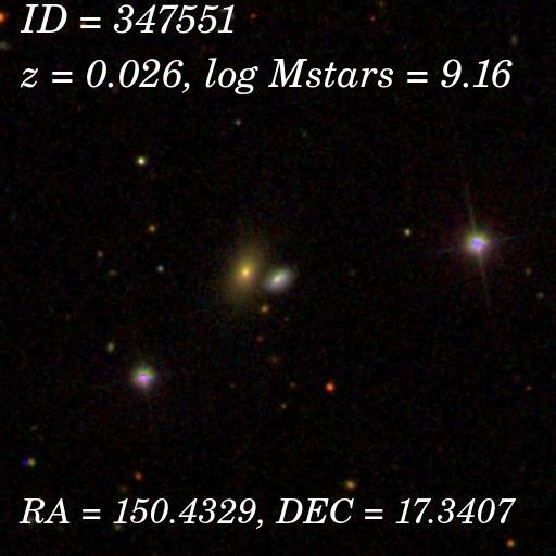
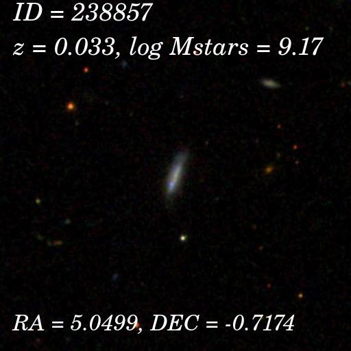
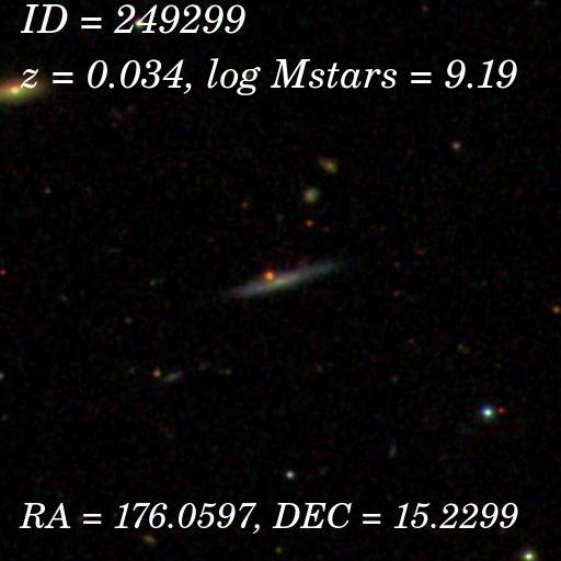
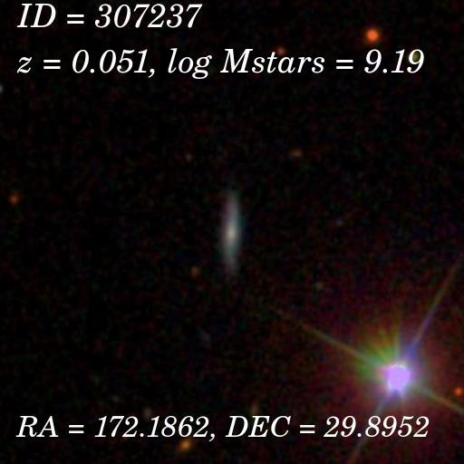
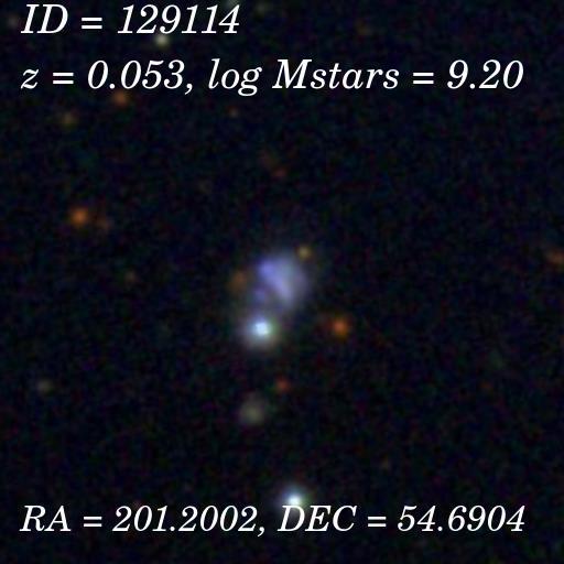
Figure 24: SDSS images of a sample of 207 VYGs. All images are 100 x 100 kpc.

References

- Abazajian et al. (2009) Abazajian K. N., et al., 2009, ApJS, 182, 543
- Abraham et al. (1994) Abraham R. G., Valdes F., Yee H. K. C., van den Bergh S., 1994, ApJ, 432, 75
- Abraham et al. (1996) Abraham R. G., van den Bergh S., Glazebrook K., Ellis R. S., Santiago B. X., Surma P., Griffiths R. E., 1996, ApJS, 107, 1
- Alloin et al. (1979) Alloin D., Collin-Souffrin S., Joly M., Vigroux L., 1979, A&A, 78, 200
- Aloisi et al. (2007) Aloisi A., et al., 2007, ApJ, 667, L151
- Armus et al. (1987) Armus L., Heckman T., Miley G., 1987, AJ, 94, 831
- Asari et al. (2007) Asari N. V., Cid Fernandes R., Stasińska G., Torres-Papaqui J. P., Mateus A., Sodré L., Schoenell W., Gomes J. M., 2007, MNRAS, 381, 263
- Baldwin et al. (1981) Baldwin J. A., Phillips M. M., Terlevich R., 1981, PASP, 93, 5
- Balogh et al. (2009) Balogh M. L., et al., 2009, MNRAS, 398, 754
- Barnard (1945) Barnard G. A., 1945, Nature, 156, 783
- Behroozi et al. (2013) Behroozi P. S., Wechsler R. H., Conroy C., 2013, ApJ, 770, 57
- Belfiore et al. (2015) Belfiore F., et al., 2015, MNRAS, 449, 867
- Belfiore et al. (2017) Belfiore F., et al., 2017, MNRAS, 469, 151
- Bernardi et al. (2019) Bernardi M., Domínguez Sánchez H., Brownstein J. R., Drory N., Sheth R. K., 2019, MNRAS, 489, 5633
- Bishop (2006) Bishop C. M., 2006, Pattern Recognition and Machine Learning. Springer, http://research.microsoft.com/en-us/um/people/cmbishop/prml/
- Blanton et al. (2003) Blanton M. R., et al., 2003, AJ, 125, 2348
- Blanton et al. (2005) Blanton M. R., et al., 2005, AJ, 129, 2562
- Borne et al. (2000) Borne K. D., Bushouse H., Lucas R. A., Colina L., 2000, ApJ, 529, L77
- Bressan et al. (1993) Bressan A., Fagotto F., Bertelli G., Chiosi C., 1993, A&AS, 100, 647
- Brinchmann et al. (2004) Brinchmann J., Charlot S., White S. D. M., Tremonti C., Kauffmann G., Heckman T., Brinkmann J., 2004, MNRAS, 351, 1151
- Bruzual & Charlot (2003) Bruzual G., Charlot S., 2003, MNRAS, 344, 1000
- Calzetti et al. (2000) Calzetti D., Armus L., Bohlin R. C., Kinney A. L., Koornneef J., Storchi-Bergmann T., 2000, ApJ, 533, 682
- Cardelli et al. (1989) Cardelli J. A., Clayton G. C., Mathis J. S., 1989, ApJ, 345, 245
- Cardoso et al. (2019) Cardoso L. S. M., Gomes J. M., Papaderos P., 2019, A&A, 622, A56
- Casasola et al. (2020) Casasola V., et al., 2020, A&A, 633, A100
- Catinella et al. (2010) Catinella B., et al., 2010, MNRAS, 403, 683
- Cattaneo et al. (2011) Cattaneo A., Mamon G. A., Warnick K., Knebe A., 2011, A&A, 533, A5
- Chabrier (2003) Chabrier G., 2003, PASP, 115, 763
- Charlot & Fall (2000) Charlot S., Fall S. M., 2000, ApJ, 539, 718
- Cid Fernandes et al. (2005) Cid Fernandes R., Mateus A., Sodré L., Stasińska G., Gomes J. M., 2005, MNRAS, 358, 363
- Conselice et al. (2000) Conselice C. J., Bershady M. A., Jangren A., 2000, ApJ, 529, 886
- Contreras Ramos et al. (2011) Contreras Ramos R., et al., 2011, ApJ, 739, 74
- Darg et al. (2010) Darg D. W., et al., 2010, MNRAS, 401, 1043
- De Lucia et al. (2006) De Lucia G., Springel V., White S. D. M., Croton D., Kauffmann G., 2006, MNRAS, 366, 499
- Di Matteo et al. (2008) Di Matteo P., Bournaud F., Martig M., Combes F., Melchior A. L., Semelin B., 2008, A&A, 492, 31
- Di Matteo et al. (2009) Di Matteo P., Pipino A., Lehnert M. D., Combes F., Semelin B., 2009, A&A, 499, 427
- Dinerstein (1990) Dinerstein H. L., 1990, in Thronson Jr. H. A., Shull J. M., eds, Astrophysics and Space Science Library Vol. 161, The Interstellar Medium in Galaxies. pp 257–285, doi:10.1007/978-94-009-0595-5_10
- Domínguez Sánchez et al. (2018) Domínguez Sánchez H., Huertas-Company M., Bernardi M., Tuccillo D., Fischer J. L., 2018, MNRAS, 476, 3661
- Domínguez et al. (2013) Domínguez A., et al., 2013, ApJ, 763, 145
- Dressler et al. (2018) Dressler A., Kelson D. D., Abramson L. E., 2018, ApJ, 869, 152
- Ellison et al. (2018) Ellison S. L., Catinella B., Cortese L., 2018, MNRAS, 478, 3447
- Engelbracht et al. (2008) Engelbracht C. W., Rieke G. H., Gordon K. D., Smith J. D. T., Werner M. W., Moustakas J., Willmer C. N. A., Vanzi L., 2008, ApJ, 678, 804
- Erguler (2016) Erguler K., 2016, Barnard: Barnard’s Unconditional Test. https://CRAN.R-project.org/package=Barnard
- Fagotto et al. (1994a) Fagotto F., Bressan A., Bertelli G., Chiosi C., 1994a, A&AS, 104, 365
- Fagotto et al. (1994b) Fagotto F., Bressan A., Bertelli G., Chiosi C., 1994b, A&AS, 105, 29
- Ferrari et al. (2015) Ferrari F., de Carvalho R. R., Trevisan M., 2015, ApJ, 814, 55
- Ferreras et al. (2019) Ferreras I., et al., 2019, MNRAS, 489, 608
- Fisher (1935) Fisher R. A., 1935, Journal of the Royal Statistical Society, 98, 39–
- Florido et al. (2015) Florido E., Zurita A., Pérez I., Pérez-Montero E., Coelho P. R. T., Gadotti D. A., 2015, A&A, 584, A88
- Fraley & Raftery (2002) Fraley C., Raftery A. E., 2002, Journal of the American Statistical Association, 97, 611
- Fraley et al. (2012) Fraley C., Raftery A. E., Murphy T. B., Scrucca L., 2012, mclust Version 4 for R: Normal Mixture Modeling for Model-Based Clustering, Classification, and Density Estimation
- Girardi et al. (1996) Girardi L., Bressan A., Chiosi C., Bertelli G., Nasi E., 1996, A&AS, 117, 113
- Gnedin (2000) Gnedin N. Y., 2000, ApJ, 542, 535
- Hamilton & Tegmark (2004) Hamilton A. J. S., Tegmark M., 2004, MNRAS, 349, 115
- Hamming (1998) Hamming R. W., 1998, Digital filters, 3 edn. Dover, Mineola, N.Y.
- Haynes et al. (2011) Haynes M. P., et al., 2011, AJ, 142, 170
- Haynes et al. (2018) Haynes M. P., et al., 2018, ApJ, 861, 49
- Hirschmann et al. (2015) Hirschmann M., Naab T., Ostriker J. P., Forbes D. A., Duc P.-A., Davé R., Oser L., Karabal E., 2015, MNRAS, 449, 528
- Hjorth et al. (2014) Hjorth J., Gall C., Michałowski M. J., 2014, ApJ, 782, L23
- Ho et al. (2011) Ho D. E., Imai K., King G., Stuart E. A., 2011, Journal of Statistical Software, 42, 1
- Hopkins et al. (2010) Hopkins P. F., et al., 2010, ApJ, 715, 202
- Hopkins et al. (2013) Hopkins P. F., Cox T. J., Hernquist L., Narayanan D., Hayward C. C., Murray N., 2013, MNRAS, 430, 1901
- Izotov & Thuan (1998) Izotov Y. I., Thuan T. X., 1998, ApJ, 497, 227
- Izotov & Thuan (2004) Izotov Y. I., Thuan T. X., 2004, ApJ, 616, 768
- Izotov et al. (2011) Izotov Y. I., Guseva N. G., Thuan T. X., 2011, ApJ, 728, 161
- Izotov et al. (2014) Izotov Y. I., Guseva N. G., Fricke K. J., Henkel C., 2014, A&A, 561, A33
- Izotov et al. (2018) Izotov Y. I., Thuan T. X., Guseva N. G., Liss S. E., 2018, MNRAS, 473, 1956
- Izotov et al. (2019) Izotov Y. I., Thuan T. X., Guseva N. G., 2019, MNRAS, 483, 5491
- Joseph & Wright (1985) Joseph R. D., Wright G. S., 1985, MNRAS, 214, 87
- Kauffmann et al. (2003) Kauffmann G., et al., 2003, MNRAS, 341, 33
- Kewley et al. (2001) Kewley L. J., Dopita M. A., Sutherland R. S., Heisler C. A., Trevena J., 2001, ApJ, 556, 121
- Knobel et al. (2015) Knobel C., Lilly S. J., Woo J., Kovač K., 2015, ApJ, 800, 24
- Kobayashi (2004) Kobayashi C., 2004, MNRAS, 347, 740
- Komatsu et al. (2011) Komatsu E., et al., 2011, ApJS, 192, 18
- Kreckel et al. (2013) Kreckel K., et al., 2013, ApJ, 771, 62
- Kroupa (2001) Kroupa P., 2001, MNRAS, 322, 231
- La Barbera et al. (2010) La Barbera F., De Carvalho R. R., De La Rosa I. G., Gal R. R., Swindle R., Lopes P. A. A., 2010, AJ, 140, 1528
- La Barbera et al. (2012) La Barbera F., Ferreras I., de Carvalho R. R., Bruzual G., Charlot S., Pasquali A., Merlin E., 2012, MNRAS, 426, 2300
- Le Borgne et al. (2003) Le Borgne J.-F., et al., 2003, A&A, 402, 433
- Lintott et al. (2011) Lintott C., et al., 2011, MNRAS, 410, 166
- Lotz et al. (2004) Lotz J. M., Primack J., Madau P., 2004, AJ, 128, 163
- Madau & Dickinson (2014) Madau P., Dickinson M., 2014, ARA&A, 52, 415
- Mahajan et al. (2011) Mahajan S., Mamon G. A., Raychaudhury S., 2011, MNRAS, 416, 2882
- Mahalanobis (1936) Mahalanobis P. C., 1936, Proceedings of the National Institute of Sciences (Calcutta), 2, 49
- Mamon (1992) Mamon G. A., 1992, ApJ, 401, L3
- Mamon (2000) Mamon G. A., 2000, in Combes F., Mamon G. A., Charmandaris V., eds, Astronomical Society of the Pacific Conference Series Vol. 197, Dynamics of Galaxies: from the Early Universe to the Present. p. 377 (arXiv:astro-ph/9911333)
- Mamon et al. (2020) Mamon G. A., Trevisan M., Thuan T. X., Gallazzi A., Davé R., 2020, MNRAS, 492, 1791 (Paper II)
- Maraston (2005) Maraston C., 2005, MNRAS, 362, 799
- Maraston & Strömbäck (2011) Maraston C., Strömbäck G., 2011, MNRAS, 418, 2785
- Marino et al. (2013) Marino R. A., et al., 2013, A&A, 559, A114
- McGee et al. (2011) McGee S. L., Balogh M. L., Wilman D. J., Bower R. G., Mulchaey J. S., Parker L. C., Oemler A., 2011, MNRAS, 413, 996
- Momcheva et al. (2013) Momcheva I. G., Lee J. C., Ly C., Salim S., Dale D. A., Ouchi M., Finn R., Ono Y., 2013, AJ, 145, 47
- Moster et al. (2013) Moster B. P., Naab T., White S. D. M., 2013, MNRAS, 428, 3121
- Mutch et al. (2013) Mutch S. J., Croton D. J., Poole G. B., 2013, MNRAS, 435, 2445
- Nair & Abraham (2010) Nair P. B., Abraham R. G., 2010, ApJS, 186, 427
- Pagel et al. (1979) Pagel B. E. J., Edmunds M. G., Blackwell D. E., Chun M. S., Smith G., 1979, MNRAS, 189, 95
- Pearson et al. (2019) Pearson W. J., et al., 2019, A&A, 631, A51
- Peng et al. (2010) Peng Y.-j., et al., 2010, ApJ, 721, 193
- Pettini & Pagel (2004) Pettini M., Pagel B. E. J., 2004, MNRAS, 348, L59
- Pietrinferni et al. (2004) Pietrinferni A., Cassisi S., Salaris M., Castelli F., 2004, ApJ, 612, 168
- Pietrinferni et al. (2006) Pietrinferni A., Cassisi S., Salaris M., Castelli F., 2006, ApJ, 642, 797
- Pilyugin (2000) Pilyugin L. S., 2000, A&A, 362, 325
- Pilyugin (2001) Pilyugin L. S., 2001, A&A, 369, 594
- Pilyugin & Grebel (2016) Pilyugin L. S., Grebel E. K., 2016, MNRAS, 457, 3678
- Pilyugin & Thuan (2005) Pilyugin L. S., Thuan T. X., 2005, ApJ, 631, 231
- Pilyugin et al. (2018) Pilyugin L. S., Grebel E. K., Zinchenko I. A., Nefedyev Y. A., Shulga V. M., Wei H., Berczik P. P., 2018, A&A, 613, A1
- R Core Team (2015) R Core Team 2015, R: A Language and Environment for Statistical Computing. R Foundation for Statistical Computing, Vienna, Austria, https://www.R-project.org
- Renzini (2020) Renzini A., 2020, MNRAS, 495, L42
- Rosenbaum & Rubin (1983) Rosenbaum P. R., Rubin D. B., 1983, Biometrika, 70, 41
- Saintonge et al. (2011) Saintonge A., et al., 2011, MNRAS, 415, 61
- Saintonge et al. (2016) Saintonge A., et al., 2016, MNRAS, 462, 1749
- Sánchez-Blázquez et al. (2006) Sánchez-Blázquez P., et al., 2006, MNRAS, 371, 703
- Sanders et al. (2017) Sanders R. L., Shapley A. E., Zhang K., Yan R., 2017, ApJ, 850, 136
- Savage & Mathis (1979) Savage B. D., Mathis J. S., 1979, ARA&A, 17, 73
- Skillman & Kennicutt (1993) Skillman E. D., Kennicutt Jr. R. C., 1993, ApJ, 411, 655
- Springob et al. (2005) Springob C. M., Haynes M. P., Giovanelli R., Kent B. R., 2005, ApJS, 160, 149
- Storey & Zeippen (2000) Storey P. J., Zeippen C. J., 2000, MNRAS, 312, 813
- Sutter et al. (2012) Sutter P. M., Lavaux G., Wandelt B. D., Weinberg D. H., 2012, ApJ, 761, 44
- Swanson et al. (2008) Swanson M. E. C., Tegmark M., Hamilton A. J. S., Hill J. C., 2008, MNRAS, 387, 1391
- Taylor (2005) Taylor M. B., 2005, in Shopbell P., Britton M., Ebert R., eds, Astronomical Society of the Pacific Conference Series Vol. 347, Astronomical Data Analysis Software and Systems XIV. p. 29
- Tempel et al. (2014) Tempel E., Stoica R. S., Martínez V. J., Liivamägi L. J., Castellan G., Saar E., 2014, MNRAS, 438, 3465
- Thomas et al. (2010) Thomas D., Maraston C., Schawinski K., Sarzi M., Silk J., 2010, MNRAS, 404, 1775
- Thomas et al. (2011) Thomas D., Maraston C., Johansson J., 2011, MNRAS, 412, 2183
- Thuan et al. (2016) Thuan T. X., Goehring K. M., Hibbard J. E., Izotov Y. I., Hunt L. K., 2016, MNRAS, 463, 4268
- Tiwari et al. (2020) Tiwari J., Mahajan S., Singh K. P., 2020, New Ast, 81, 101417
- Tojeiro et al. (2009) Tojeiro R., Wilkins S., Heavens A. F., Panter B., Jimenez R., 2009, ApJS, 185, 1
- Tremonti et al. (2004) Tremonti C. A., et al., 2004, ApJ, 613, 898
- Trevisan et al. (2012) Trevisan M., Ferreras I., de La Rosa I. G., La Barbera F., de Carvalho R. R., 2012, ApJ, 752, L27
- Trevisan et al. (2017a) Trevisan M., Mamon G. A., Khosroshahi H. G., 2017a, MNRAS, 464, 4593
- Trevisan et al. (2017b) Trevisan M., Mamon G. A., Stalder D. H., 2017b, MNRAS, 471, L47
- Tweed et al. (2018) Tweed D. P., Mamon G. A., Thuan T. X., Cattaneo A., Dekel A., Menci N., Calura F., Silk J., 2018, MNRAS, 477, 1427 (Paper I)
- Vazdekis et al. (2010) Vazdekis A., Sánchez-Blázquez P., Falcón-Barroso J., Cenarro A. J., Beasley M. A., Cardiel N., Gorgas J., Peletier R. F., 2010, MNRAS, 404, 1639
- Vazdekis et al. (2015) Vazdekis A., et al., 2015, MNRAS, 449, 1177
- Weinmann et al. (2006) Weinmann S. M., van den Bosch F. C., Yang X., Mo H. J., 2006, MNRAS, 366, 2
- Willett et al. (2013) Willett K. W., et al., 2013, MNRAS, 435, 2835
- Woo et al. (2013) Woo J., et al., 2013, MNRAS, 428, 3306
- Wright et al. (2010) Wright E. L., et al., 2010, AJ, 140, 1868
- Yang et al. (2005) Yang X., Mo H. J., van den Bosch F. C., Jing Y. P., 2005, MNRAS, 356, 1293
- Yang et al. (2007) Yang X., Mo H. J., van den Bosch F. C., Pasquali A., Li C., Barden M., 2007, ApJ, 671, 153
- Zaritsky et al. (1994) Zaritsky D., Kennicutt Jr. R. C., Huchra J. P., 1994, ApJ, 420, 87
- Zhang et al. (2017) Zhang K., et al., 2017, MNRAS, 466, 3217
- Zhang et al. (2019) Zhang C., et al., 2019, ApJ, 884, L52
- Zhuang et al. (2019) Zhuang Y., Leaman R., van de Ven G., Zibetti S., Gallazzi A., Zhu L., Falcón-Barroso J., Lyubenova M., 2019, MNRAS, 483, 1862
- Zibetti et al. (2020) Zibetti S., Gallazzi A. R., Hirschmann M., Consolandi G., Falcón-Barroso J., van de Ven G., Lyubenova M., 2020, MNRAS, 491, 3562
- da Cunha et al. (2010) da Cunha E., Eminian C., Charlot S., Blaizot J., 2010, MNRAS, 403, 1894
- de Souza et al. (2016) de Souza R. S., et al., 2016, MNRAS, 461, 2115
- de Vaucouleurs (1963) de Vaucouleurs G., 1963, ApJS, 8, 31
- van Zee et al. (1998) van Zee L., Westpfahl D., Haynes M. P., Salzer J. J., 1998, AJ, 115, 1000
- von der Linden et al. (2010) von der Linden A., Wild V., Kauffmann G., White S. D. M., Weinmann S., 2010, MNRAS, 404, 1231