Learning to Separate Clusters of Adversarial Representations
for Robust Adversarial Detection

Abstract

Deep neural networks have shown promising performances on various tasks, but they are also susceptible to incorrect predictions induced by imperceptibly small perturbations in inputs. Although a large number of previous works have been proposed to detect adversarial examples, most of them cannot effectively detect adversarial examples against adaptive whitebox attacks where an adversary has the knowledge of the victim model and the defense method. In this paper, we propose a new probabilistic adversarial detector which is effective against the adaptive whitebox attacks. From the observation that the distributions of adversarial and benign examples are highly overlapping in the output space of the last layer of the neural network, we hypothesize that this overlapping representation limits the effectiveness of existing adversarial detectors fundamentally, and we aim to reduce the overlap by separating adversarial and benign representations. To realize this, we propose a training algorithm to maximize the likelihood of adversarial representations using a deep encoder and a Gaussian mixture model. We thoroughly validate the robustness of our detectors with 7 different adaptive whitebox and blackbox attacks and 4 perturbation types $\ell_{p},p\in\{0,1,2,\infty\}$. The results show our detector improves the worst case Attack Success Ratios up to 45% (MNIST) and 27% (CIFAR10) compared to existing detectors.

1 Introduction

In the past decade, deep neural networks have achieved impressive performance on many tasks including image classification. Recently, it was discovered that imperceptibly small perturbations called adversarial examples can reduce the accuracy of classification models to almost zero without inducing semantic changes in the original images [65, 23]. A number of defense methods have been proposed to overcome the attack of adversarial examples, including the ones of improving the robustness of inference under input perturbation [27, 77, 51, 62, 14, 63] and detecting adversarial vs clean examples [18, 22, 26, 56, 73, 69, 48]. Despite the effectiveness of those methods under blackbox attack scenarios, many of them are ineffective under adaptive whitebox scenarios in which the adversary can create sophisticated adversarial examples using the full knowledge of the defender [8, 3].

In this paper, we propose a robust adversarial detector under the adaptive whitebox threat model, providing a new perspective to examine and address adversarial attacks in the representation space – the output from the last layer in a neural network (before softmax normalization). In our preliminary experiment (Section 3.1), we find the distribution of adversarial examples overlaps the distribution of benign examples in the representation space. The overlap between benign and adversarial distributions makes it hardly possible to distinguish adversarial examples through distance-based detection methods in the representation space. This observation motivates us to explore the possibility to separate benign and adversarial distributions in the representation space. This presents a novel perspective on adversarial examples different from previous perspectives which view them simply as random examples that fall onto the incorrect side of the decision boundary of classifiers  [22, 26].

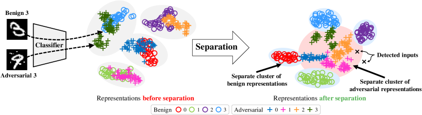
Figure 1: Benign (circles) and adversarial ($+$) representations from a classifier. We observe that in the representation space, the adversarial distribution overlap with the benign distribution before our defense method is used (Left). After our method is used, adversarial examples are well separated from benign examples facilitating the robust detection of attacks (Right).

We describe our idea in Figure 1 which shows the representations of benign and adversarial examples. We prepare a pre-trained deep neural network that classifies MNIST[40] dataset of hand-written digits images. We generate adversarial examples on the classifier and visualize the representations of them reducing its dimension in 2D plane. In Figure 1 (left), the circles are the representations of benign examples and the plus sign indicate the representations of adversarial examples. Colors denote the predicted labels. Contrary to the popular belief that adversarial examples are random samples, representations of adversarial examples form their own clusters (clusters of $+$ with same colors), rather than surrounding benign clusters (clusters of circles with same colors). Furthermore, for each label, its benign and adversarial clusters overlap each other, which makes it difficult to detect adversarial examples from their representations. It is therefore desirable that adversarial and benign examples from separate clusters in the representation space such that we can use distance-based measures (or equivalently, likelihood-based measures) to detect adversarial examples (Figure 1 right, black $\times$). To achieve this, we propose a deep encoder which maximizes class conditional likelihood assuming Gaussian mixture model in the representation space. We introduce an additional cluster for the adversarial representations, and also maximize its class conditional likelihoods.

To the best of our knowledge, it is the first attempt in the literature that adversarial attacks are explained by overlapping distributions of representations and consequently addressed by separating the clusters. Existing detectors focus only on clusters of benign representations [43, 57] and do not attempt to model adversarial representations. Similar to our idea of clusters of adversarial representations, a prior work [35] defines a common property of adversarial examples as a mathematical function but does not suggest a defense method.

By learning the separate clusters of benign and adversarial representations, we encourage a neural network to learn distinct representations of benign examples that are clearly distinguished from adversarial representations, which enables robust adversarial detection based on distances in the representation space.

We summarize our contributions as follows.

• We make new observations that adversarial examples present themselves as clusters in the representation space that overlap with benign clusters, and posit that it poses a fundamental limitation on the detection of adversarial examples in the previous defense methods.

• We propose a new robust adversarial detector and a training algorithm for it which effectively detects adversarial examples under an adaptive whitebox threat model by estimating separate clusters of adversarial representations.

• We conduct comprehensive experiments against 7 adaptive whitebox and blackbox attacks with 4 different perturbation types. Our approach improves the worst-case detection performance (Attack Success Ratio) by up to 45% (MNIST) and 27% (CIFAR10) compared to the state-of-the-art detectors.

2 Background

2.1 Neural network

Deep Neural Network (DNN) is a function, $H_{\theta}:\mathbf{X}\rightarrow\mathbf{Z}$, which maps $n$ dimensional input space $\mathbf{X}$ to $m$ dimensional output space $\mathbf{Z}$. In general, DNN is a composition of many sub-functions $h_{i}$ which are also called layers, such that $H_{\theta}(\mathbf{x})=h_{L}\circ h_{L-1}\circ\cdots\circ h_{1}(\mathbf{x})$. The popular examples of layers include fully connected layers and convolutional layers followed by activation functions such as ReLU, sigmoid or linear. Representations are outputs of each layer, $\cup_{i=1}^{L}h_{i}\circ h_{i-1}\cdots\circ h_{1}(\mathbf{x})$, given an input $\mathbf{x}$. In this paper, our main interest is the representation of the last layer $H_{\theta}(\mathbf{x})=h_{L}\circ h_{L-1}\cdots\circ h_{1}(\mathbf{x})$.

For k-class classification tasks, practitioners build a classifier $f:\mathbf{X}\rightarrow\mathbf{Y}$ multiplying $k\times m$ matrix $\mathbf{W}$ to $H_{\theta}(\mathbf{x})$ so that $g(\mathbf{x})=\mathbf{W}H_{\theta}(\mathbf{x})=[g_{1}(\mathbf{x}),g_{2}(\mathbf{x}),\cdots,g_{k}(\mathbf{x})]^{T}$. Then, $g_{i}(\mathbf{x})$ are normalized by softmax function and becomes $f_{i}(\mathbf{x})=e^{g_{i}(\mathbf{x})}/\sum_{j=1}^{k}e^{g_{j}(\mathbf{x})}$. We can interpret $f_{i}(\mathbf{x})$ as a classification probability of $\mathbf{x}$ to label $i$, $p(y=i|\mathbf{x})$ because, $f_{i}(\mathbf{x})$ ranges from 0 to 1 and $\sum_{i=1}^{k}f_{i}(\mathbf{x})=1$. Then, classification label of $\mathbf{x}$ is $\hat{y}=\operatorname*{arg\,max}_{i}f_{i}(\mathbf{x})$.

To train the classifier with training data $\mathcal{D}$, we compute loss function $\mathcal{L}(f(\mathbf{x}),y),(\mathbf{x},y)\in\mathcal{D}$, which indicates how the classification differs from the correct label $y$. Then we update parameters $\theta$ and $W$ so that resulting $f$ minimizes the loss. In particular, we use gradient descent method with back-propagation algorithms.

2.2 Adversarial evasion attack

Adversarial evasion attacks modify an input $\mathbf{x}$ by adding imperceptible perturbation $\delta$ in test time, so that $\mathbf{x}+\delta$ is misclassified to a wrong label, although the original $\mathbf{x}$ is classified correctly. Formally, the main objective of attacks is to find $\delta$ satisfying,

$$y=\operatorname*{arg\,max}_{i}f_{i}(\mathbf{x})\land y\neq\operatorname*{arg\,max}_{i}f_{i}(\mathbf{x}+\delta)$$ (1)

$$s.t.\;||\delta||_{p}\leq\epsilon,\,\,(\mathbf{x},y)\in\mathcal{D}$$ (2)

The first statement implies the condition of misclassification of perturbed image $\mathbf{x}+\delta$, and the second statement constraints the size of the perturbation $\delta$ to be smaller than $\epsilon$ so that the original semantics of $\mathbf{x}$ is not changed. $||\delta||_{p}$ is called $p$-norm or $\ell_{p}$ of $\mathbf{\delta}$, and it is computed as,

$$||\delta||_{p}=\sqrt[p]{\sum_{i}|\delta_{i}|^{p}}$$

Depending on attack constraints and semantics of $\mathbf{x}$, the representative $p$ values can be 0, 1, 2 or $\infty$. In particular $\ell_{0}$ of $\delta$ restricts the number of non-zero elements, and $\ell_{\infty}$ of $\delta$ restricts $\max_{i}|\delta_{i}|$, the maximum value of changes.

Since a first discovery of adversarial attack [65], many variants of evasion attacks are developed. They can be categorized into two classes depending on information adversaries can utilize in finding $\delta$, whitebox attacks and blackbox attacks.

Whitebox attack.

In whitebox attack model, adversary can access the victim classifier $f(\mathbf{x})$ and observe the output and representations of $f(\mathbf{x})$. In particular, whitebox attacks leverage backpropagation algorithm to compute gradient of classification loss, $\nabla_{\mathbf{x}}\mathcal{L}(f(\mathbf{x}),y)$ and modify $\mathbf{x}$ based on the gradient.

$\bullet$ Fast Gradient Sign Method (FGSM) [23] is a basic whitebox attack method which generates an adversarial example as,

$$\mathbf{x_{\text{adv}}}=\mathbf{x}+\epsilon\,\text{sign}(\nabla_{\mathbf{x}}\mathcal{L}(f(\mathbf{x}),y))$$

FGSM increases the classification loss by adding $\delta=\epsilon\,\text{sign}(\nabla_{\mathbf{x}}\mathcal{L}(f(\mathbf{x}),y))$ to the original $\mathbf{x}$ so that $\mathbf{x_{\text{adv}}}$ is misclassified to wrong label other than $y$. By taking sign of gradient, FGSM satisfies $||\delta||_{\infty}=||\epsilon\,\text{sign}(\nabla_{\mathbf{x}}\mathcal{L}(f(\mathbf{x}),y))||_{\infty}=\epsilon\leq\epsilon$.

$\bullet$ Projected Gradient Descent (PGD) is a stronger attack than FGSM which can be considered as applying FGSM multiple times. PGD attack [51] has three attack parameters, $\epsilon$, $\alpha$ and $k$. The parameter $\epsilon$ constraints the size of $\delta$, and $\alpha$ is a size of single step perturbation of FGSM. $k$ is the number of application of FGSM attack. PGD can be represented as follows.

$$\mathbf{x^{t+1}}=\text{clip}_{(\mathbf{x},\epsilon)}(\mathbf{x^{t}}+\alpha\,\text{sign}(\nabla_{\mathbf{x}}\mathcal{L}(f(\mathbf{x^{t}}),y))$$ (3)

$$\mathbf{x^{0}}=\mathbf{x}\,$$ (4)

$$\mathbf{x}_{\text{adv}}=\mathbf{x}^{k}$$ (5)

The sign function is an element-wise function which is 1 if an input is positive otherwise -1. $\text{clip}_{(\mathbf{x},\epsilon)}(\mathbf{x}^{\prime})$ is an element-wise function which enforces $||\delta||_{\infty}=||\mathbf{x}_{\text{adv}}-\mathbf{x}||_{\infty}\leq\epsilon$. It is defined as,

$$\text{clip}_{(x_{i},\epsilon)}(x^{\prime}_{i})=\begin{cases}x^{\prime}_{i}&\text{if }|x^{\prime}_{i}-x_{i}|\leq\epsilon\\ \epsilon\,\text{sign}(x^{\prime}_{i}-x_{i})&\text{otherwise}\end{cases}$$

The above attacks are explained in the perspective of $\ell_{\infty}$ perturbation, however they can be extended to other perturbations $\ell_{p}$ by replacing the sign and clip function to different vector projection and normalization functions. Also attacks can induce a specific target wrong label (targeted attack) rather than arbitrary labels as above (untargeted attack). For target label $y_{\text{target}}$, we replace $\mathcal{L}(f(\mathbf{x^{t}}),y))$ to $\mathcal{L}(f(\mathbf{x^{t}}),y_{\text{target}}))$ and negate the sign of perturbation to minimize the loss,

$$\mathbf{x^{t+1}}=\text{clip}_{(\mathbf{x},\epsilon)}(\mathbf{x^{t}}-\alpha\,\text{sign}(\nabla_{\mathbf{x}}\mathcal{L}(f(\mathbf{x^{t}}),y_{\text{target}}))$$ (6)

Especially, we call a circumstance adaptive whitebox attack model if an adversary also knows victim’s defense mechanism in addition to the classifier $f(\mathbf{x})$. In the adaptive whitebox attack model, attacks can be adapted to a specific defense by modifying their objective function $\mathcal{L}(f(\mathbf{x^{t}}),y)$ as suggested by a prior work [8]. For instance, assume a defense detects adversarial examples if its defense metric $q:\mathbf{X}\rightarrow\mathbb{R}$ is too low compared to benign data $(\mathbf{x},y)\in\mathcal{D}$. Then, an attack can be adapted to the defense by adding $q(\mathbf{x})$ to the base objective function $\mathcal{L}(f(\mathbf{x^{t}}),y)$ so that,

$$\mathcal{L}_{\text{adapt}}(f(\mathbf{x^{t}}),y)=\mathcal{L}(f(\mathbf{x^{t}}),y)+q(\mathbf{x})$$ (7)

It is important to evaluate defense mechanisms in an adaptive whitebox attack model, although the adaptive whitebox attack model is not realistic assuming adversary’s complete access to victims, because it evaluates robustness of the defenses more thoroughly.

Blackbox attack.

In blackbox attack model, an adversary only observes partial information about the victim such as training data, classification probabilities $p(\mathbf{y}|\mathbf{x})$ or classification label $\hat{y}=arg\max_{i}f_{i}(\mathbf{x})$. It tries to generate adversarial examples based on the limited information. We introduce representative three blackbox attacks here.

$\bullet$ Transfer attack [46] only assumes an access to training data $\mathcal{D}$ of a victim classifier $f(\mathbf{x})$. An adversary trains their surrogate classifier $f_{s}(\mathbf{x})$ with $\mathcal{D}$ and generates adversarial examples $\mathbf{x}_{\text{adv}}$ on $f_{s}$. Then the adversary applies $\mathbf{x}_{\text{adv}}$ to the victim classifier $f(\mathbf{x})$. It leverages a property of adversarial examples called transferability which means adversarial examples generated from a classifier successfully induce wrong labels on other classifiers in high probability.

$\bullet$ Natural Evolution Strategy (NES) [70] assumes an access to classification probabilities of an input, $f(\mathbf{x})$. Based on the classification probabilities of $n$ neighbor inputs which are sampled by Gaussian distribution $N(\mathbf{x},\sigma\mathbf{I})$ where $\mathbf{I}$ is an identity matrix, it estimates gradient of expected classification probability as follows,

$$\nabla_{\mathbf{x}}\mathbb{E}[f_{i}(\mathbf{x})]=\frac{1}{\sigma n}\sum_{i=1}^{n}f_{i}(\mathbf{x}_{i}),\;\mathbf{x}_{i}\sim N(\mathbf{x},\sigma\mathbf{I})$$

Then, it follows the same attack process with whitebox attack replacing the backpropagated gradient $\nabla_{\mathbf{x}}\mathcal{L}(f(\mathbf{x^{t}}),y))$ with the estimated gradient $\nabla_{\mathbf{x}}\mathbb{E}[f_{i}(\mathbf{x})]$ to increase classification probability of $\mathbf{x}$ to a label $i$.

$\bullet$ Boundary attack [5] only assumes an access to a classification label, $\hat{y}=arg\max_{i}f(\mathbf{x})$. In contrast to other attacks find $\delta$ starting from $(\mathbf{x},y)\in\mathcal{D}$, boundary attack starts from a uniform sample in valid input space where $y\neq arg\max_{i}f(\mathbf{x}_{0})$. In a nutshell, after finding $\mathbf{x}_{0}$, the attack iteratively finds $\mathbf{x}_{t+1}$ in the neighborhood of $\mathbf{x}_{t}$, so that $y\neq arg\max_{i}f(\mathbf{x}_{t+1})$ is still satisfied while minimizing $||\mathbf{x}-\mathbf{x}_{t+1}||_{2}<||\mathbf{x}-\mathbf{x}_{t}||_{2}$. After $k$ iterations, $\mathbf{x}_{k}$ approaches very close to $\mathbf{x}$ while classified to wrong label.

2.3 Threat model

Problem and threat model.

A problem we deal with in this paper is to find a neural network model which robustly detects adversarial examples so that main classification tasks are not compromised by adversaries. As a metric of the detection performance, we define Attack Success Ratio $\mathcal{S}(f,q)$, similar to a prior work [75] (lower is better):

$$\begin{aligned} \mathcal{S}(f,q)=\mathbb{E}_{(\mathbf{x},y)\sim\mathcal{D}}&[\textbf{1}\{\exists{||\delta||_{p}\leq\epsilon}\\ &\mbox{s.t.}\;f(\mathbf{x}+\delta)\neq f(\mathbf{x})=y,\;q(\mathbf{x})\leq 0\}]\end{aligned}$$ (8)

$f$ is a classifier which outputs a class label and $q$ is a detector which is greater than 0 if an input is adversarial. $\mathbf{1}\{\textit{cond}\}$ is 1 if cond is true, otherwise 0. So $\mathcal{S}(f,q)$ is a proportion of $(\mathbf{x},y)\in\mathcal{D}$ where adversaries can find $\mathbf{\delta}$ which misleads $f$ and bypasses $q$ , over the entire data points in $\mathcal{D}$. Therefore our objective is to find neural networks lowering $\mathcal{S}(f,q)$.

We assume adaptive whitebox adversaries who know everything of victim models and defense mechanisms. It is an attack model suggested in prior works [4, 8] where we can analyze effective robustness of a defense method. For example, adversaries can compute gradients to generate adversarial examples, and see intermediate values of victim models. The objective of the adversaries is to fool our detector and classification, increasing $\mathcal{S}(f,q)$. On the other hand, defenders can change the parameters of victim models to resist against the adversaries in a training phase. However, after the training phase, the defenders do not have control of the victim models so it is the most challenging condition to defenders. We also consider blackbox attacks where the adversaries do not have knowledge of the victim models to ensure that our defense does not depend on obfuscated gradients [3].

3 Approach

In this section, we propose an adversarial detector against adaptive whitebox adversaries. First, we empirically demonstrate clusters of adversarial representations in neural networks (Section 3.1). In addition, we find the adversarial clusters highly overlap with benign representations, which makes it hardly possible for any existing detectors to detect them based on the representations. Motivated by the fundamental limitation, we introduce a new adversarial detector and a training method (Section 3.2) which separates the adversarial representations in a new cluster to minimize the overlaps with benign representations. To the best of our knowledge, it is the first time to identify adversarial examples as clusters of representations and deal with them by cluster separations. For detailed comparisons to existing approaches, we refer readers to the related work section (Section 4).

3.1 Motivation

In this section, we demonstrate an experiment where we identify clusters of adversarial representations and get motivated to separate them from benign representations. We prepare MNIST[40] training data $\mathcal{D}$ which contains hand-written digit images form 0 to 9 ($k=10$ classes), and a deep neural network $H_{\mathbf{\theta}}:\mathbf{X}\rightarrow\mathbb{R}^{k}$ initialized with parameters $\mathbf{\theta}$. $H_{\mathbf{\theta}}$ maps $\mathbf{x}$ to a representation $\mathbf{z}$ in $k$ dimensional space. We also assign $\mathbf{\mu}_{0},\mathbf{\mu}_{1},\cdots,\text{and}\;\mathbf{\mu}_{k-1}$ in the representation space, and let $\mathbf{\mu}_{i}$ be a center of representations $H_{\theta}(\mathbf{x}_{y\texttt{=}i})$, where $\mathbf{x}_{y=i}$ is defined as $\mathbf{x}$ whose label is $i$, $(\mathbf{x},y=i)\in\mathcal{D}$. In particular, we let $\mu_{i}$ be an one hot encoding of label $i$ as similar with a prior work [21].

We train $H_{\theta}$ by updating the parameters $\mathbf{\theta}$ so that $H_{\theta}(\mathbf{x}_{y=i})$ is clustered around $\mathbf{\mu}_{i}$ with a training objective,

$$\hat{\theta}=\operatorname*{arg\,min}_{\theta}\mathcal{L}(\theta;\mathcal{D})$$ (9)

$$\mathcal{L}(\theta;\mathcal{D})=\sum_{(\mathbf{x},y)\in\mathcal{D}}||H_{\mathbf{\theta}}(\mathbf{x})-\mathbf{\mu}_{y}||_{2}$$ (10)

Optimizing above loss, we can find new parameters $\hat{\theta}$ that minimize Euclidean distance between $H_{\hat{\theta}}(\mathbf{x}_{y\texttt{=}i})$ and $\mathbf{\mu}_{i}$. Then, we can devise a classifier $f(\mathbf{x})$ based on the distance,

$$\hat{y}=f(\mathbf{x})=\operatorname*{arg\,min}_{c}||H_{\hat{\mathbf{\theta}}}(\mathbf{x})-\mathbf{\mu}_{c}||_{2}$$

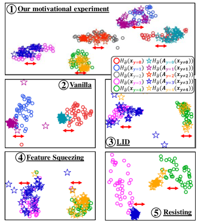
Figure 2: Overlaps of benign and adversarial clusters in a representation space of our motivational experiment (1). We also find the overlaps in representation spaces of a vanilla classifier (2) and other existing detectors (3 $\sim$ 5).

After $H_{\hat{\theta}}$ is trained, we inspect representations of benign and adversarial examples. To visualize benign representations $H_{\hat{\theta}}(\mathbf{x}),(\mathbf{x},i)\in\mathcal{D}$, we reduce the dimension of $H_{\hat{\theta}}(\mathbf{x})$ to 2 dimensional space with t-SNE [50] algorithm. We plot the result in of Figure 2. We can check that $H_{\hat{\theta}}(\mathbf{x}_{y=i})$ of the same class (circles with the same colors) are in the same cluster as we intended. Then we observe representations of adversarial examples $H_{\hat{\theta}}(\mathbf{A}_{{y=i}}(\mathbf{x}_{y\neq i}))$. $\mathbf{A}_{y=i}$ is an targeted attack algorithm which finds $\mathbf{\delta}$ satisfying $i=f(\mathbf{x}+\delta)$. We can derive $\mathbf{A}_{y=i}$ by modifying PGD attack (Equation 6) replacing the attack loss $\mathcal{L}$ with $||H_{\mathbf{\hat{\theta}}}(\mathbf{x}+\mathbf{\delta})-\mathbf{\mu}_{i}||_{2}$. The adversarial examples are generated with $\ell_{\infty}$ 0.3 perturbations and $H_{\hat{\theta}}(\mathbf{A}_{{y=i}}(\mathbf{x}_{y\neq i}))$ are also plotted as stars in of Figure 2. Not only the adversarial representations $H_{\hat{\theta}}(\mathbf{A}_{y\texttt{=}i}(\mathbf{x}_{y\neq i}))$ are close to centers $\mathbf{\mu}_{i}$ of the misleading target class $i$, but the adversarial representations also forms their own clusters near $\mathbf{\mu}_{i}$. The existence of the cluster of adversarial representations is not expected, because the adversarial examples $\mathbf{A}_{{y=i}}(\mathbf{x}_{y\neq i})$ are generated from $\mathbf{x}_{y\neq i}$ of various classes $y\in\{0,1,\cdots,k-1\}-\{i\}$ which do not share visual similarity of class $i$. We also conducted similar experiments on a vanilla classifier and different detector approaches ( $\sim$ ) including LID[49], Feature Squeezing[73] Resisting [21]. We find the overlaps consistently exist in the classifier and detection models. In the perspective of adversarial detection we regard these overlaps are fundamental limitations of existing detectors, because it is impossible to detect $\mathbf{A}_{y\texttt{=}i}(\mathbf{x}_{y\neq i})$ based on the distance metric $||\mathbf{A}_{y\texttt{=}i}(\mathbf{x}_{y\neq i})-\mathbf{\mu}_{i}||_{2}$ as long as the overlaps between benign clusters and adversarial clusters exist (red arrows) in the representation space.

Therefore, we are motivated to find $H_{\theta}$ which separates benign clusters clearly distinguished from the adversarial representations (red and blue circles surrounded by dashed lines in “After our method” of Figure 3), so that distances between $\mathbf{\mu}_{i}$ and $H_{\theta}(\mathbf{x})$ can be effective metrics for detecting adversarial examples. To ensure the non-overlapping clusters, we focus on the existence of clusters of adversarial representations ( of Figure 3). If the adversarial representations truly form their own clusters, we deduce it is also possible to find $H_{\theta}$ that clusters the adversarial examples in a different location on the representation space. So we are motivated to generate adversarial examples $\mathbf{A}_{y=i}(\mathbf{x}_{y\neq i})$ in a training process and estimate $\theta^{\prime}$ which clusters adversarial representations to a separate center $\mathbf{\mu}_{k}$ ( of Figure 3).

It is our main contribution to identify , adversarial examples as a cluster in the representation space, and , separate the adversarial representations in a cluster at $\mathbf{\mu}_{k}$. Considering a cluster in the representation space as a property of $\mathbf{x}$ in the input space, clustering the adversarial representations at a center $\mu_{k}$ implies $H_{\theta^{\prime}}$ captures common properties of adversarial examples in the input space. Further separating clusters of adversarial representations from the cluster of benign representations ( of Figure 3), we claim the resulting clusters of benign representations reflect much distinct and robust properties of the benign examples compared to clusters before the separation. Note that the clustering representations of adversarial examples at $\mu_{k}$ is necessary to make sure the separation, because we can not measure how clearly two clusters are separated knowing only one of them. We support above claim in experiments where our detectors outperform existing approaches which do not consider adversarial clusters .

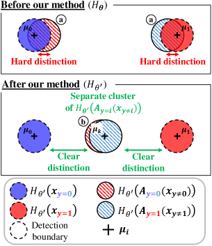
Figure 3: We find overlaps between clusters of adversarial representations and clusters of benign representations is a fundamental limitation of existing adversarial detectors (Before our method). We solve this separating benign clusters from adversarial clusters for robust adversarial detection.

3.2 Model construction

For a clear distinction between benign and adversarial representations, we introduce a probabilistic detection model and a training algorithm, which enables likelihood based robust adversarial detection. We leverage an encoder model $H_{\theta}:\mathbb{R}^{n}\rightarrow\mathbb{R}^{m}$ which is a deep neural network such as ResNet [29] and DenseNet [32] except that $H_{\mathbf{\theta}}$ is not forced to produce outputs with $m=k$ dimensions. To interpret the distance $||H_{\theta}(x)-\mathbf{\mu}_{i}||_{2}$ from the motivational experiment in a probabilistic view, we introduce $k$ Gaussian mixture model (GMM) in the representation space which contains $k$ Gaussian modes whose means and variances are parameterized with class label $y\in\{0,1,\cdots,k-1\}$:

$$\begin{aligned} p(H_{\theta}(\mathbf{x}))&=\sum_{i=0}^{k-1}p(y\texttt{=}i)p(\mathbf{z}\texttt{=}H_{\theta}(\mathbf{x})|y\texttt{=}i)\\ &=\sum_{i=0}^{k-1}p(y\texttt{=}i)N(H_{\theta}(\mathbf{x});\mathbf{u}(i),\mathbf{v}(i))\end{aligned}$$ (11)

$p(y\texttt{=}i)$ is a probability distribution of class labels $y$ of $\mathcal{D}$. In our case we can assume $p(y\texttt{=}i)$ to be equiprobable, $\forall i\in\{0,1,\cdots,k-1\},p(y\texttt{=}i)=\frac{1}{k}$, because our datasets include the same number of $\mathbf{x}$ over classes. The modes of Gaussian mixture model are Gaussian distributions $N(H_{\theta}(\mathbf{x})|\mathbf{u}(i),\mathbf{v}(i))$ whose mean $\mu_{i}$ is $\mathbf{u}(i)$ and variance $\sigma^{2}$ is $\mathbf{v}(i)$. The modes correspond to the clusters in the motivational experiment and they are illustrated with blue and red circles surrounded by dashed lines in Figure 4. We properly choose parameterizing function $\mathbf{u}$ and $\mathbf{v}$ so that Bayes error rates between the Gaussian modes should be low. Specifically,

$$l=\frac{m}{k}\in\mathbb{N}$$ (12)

$$u_{j}(y)=\begin{cases}M&\text{if }yl\leq j<(y+1)l\\ 0&\text{otherwise}\end{cases}$$ (13)

$$\mathbf{v}(y)=\mathbf{I}_{m}$$ (14)

$\mathbf{u}:\mathbb{R}\rightarrow\mathbb{R}^{m}$ returns $m$ dimensional vector given a class label $y$, whose $j^{\text{th}}$ element is defined by $u_{j}(y)$. In other words, $\mathbf{u}(y)$ returns a vector whose $l$ consecutive elements are constant $M$ starting from $yl^{\text{th}}$ element, otherwise 0. $\mathbf{u}$ can be considered as an extension of one hot encoding (if $m=k,M=1$) to be applied to $m=kl$ dimensional representations. We let $\mathbf{v}$ be a constant function which returns $m\times m$ identity matrix $\mathbf{I}_{m}$, for the efficient computation from isotropic Gaussian distributions.

From the GMM assumption, we can derive the distance $||H_{\theta}(\mathbf{x})-\mu_{i}||_{2}$ re-writing $N(H_{\theta}(\mathbf{x});\mathbf{u}(i),\mathbf{v}(i))$ in Equation 11:

$$\begin{aligned} p(H_{\theta}(\mathbf{x}))&=\sum_{i=0}^{k-1}p(y\texttt{=}i)N(H_{\theta}(\mathbf{x});\mathbf{u}(i),\mathbf{v}(i))\\ &=\sum_{i=0}^{k-1}\frac{1}{k}\frac{1}{(2\pi)^{n/2}}e^{-\frac{1}{2}||H_{\theta}(x_{i})-\mu_{y_{i}}||^{2}_{2}}\end{aligned}$$ (15)

Similar construction is introduced in prior works [43, 21, 57] and shown effective in classification tasks with flexible transformation of $H_{\theta}$. Now we can compute likelihood of the representations $p(H_{\theta}(\mathbf{x}))$ with the distances $||H_{\theta}(x_{i})-\mu_{y_{i}}||_{2}$.

Classification and Detection.

Assuming $H_{\theta^{\prime}}$ successfully clusters benign and adversarial representations in separate Gaussian modes (we explain a training method of $H_{\theta^{\prime}}$ in the following section) we can classify inputs according to Bayes classification rule, and the GMM assumption of $H_{\theta^{\prime}}$:

$$\begin{aligned} f(\mathbf{x})&=\operatorname*{arg\,max}_{y}p(y|z\texttt{=}H_{\theta^{\prime}}(\mathbf{x}))\\ &=\operatorname*{arg\,max}_{y}\frac{p(z\texttt{=}H_{\theta^{\prime}}(\mathbf{x})|y)p(y)}{p(z\texttt{=}H_{\theta^{\prime}}(\mathbf{x}))}\\ &=\operatorname*{arg\,max}_{y}p(z\texttt{=}H_{\theta^{\prime}}(\mathbf{x})|y)\\ &=\operatorname*{arg\,max}_{y}N(z\texttt{=}H_{\theta^{\prime}}(\mathbf{x});\mu_{y},\mathbf{I}_{m})\\ &=\operatorname*{arg\,min}_{y}||H_{\theta^{\prime}}(\mathbf{x})-\mu_{y}||_{2}\end{aligned}$$ (16)

After all, $\mathbf{x}$ is classified to a class label $y$ where a distance $||H_{\theta^{\prime}}(\mathbf{x})-\mathbf{\mu}_{y}||_{2}$ is minimized (Figure 4 ). The first equation is from Bayes classification rule and re-written with Bayes rule in the second equation. The $p(y)$ and denominator $H_{\theta}(\mathbf{x})$ are disappeared in the third equation because they are invariant to $y$. The conditional likelihood $p(z\texttt{=}H_{\theta}(\mathbf{x})|y)$ is re-written as a Gaussian mode $N(z\texttt{=}H_{\theta}(\mathbf{x});\mu_{y},\mathbf{I}_{m})$ in the fourth equation. Following equation is reduced by ignoring constant of Gaussian distribution and the $\operatorname*{arg\,max}_{y}$ is changed to $\operatorname*{arg\,min}_{y}$ negating the sign of the exponent of $e$ in Gaussian distribution.

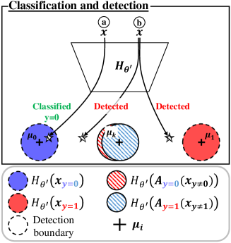
Figure 4: Classification and detection method of $H_{\theta}$. It classifies an input to a class of the closest Gaussian mode (a), or detect if the representation of input is located far from all of the benign modes (b).

We explain how $H_{\theta^{\prime}}$ detects an input $\mathbf{x}$ as an adversarial examples. It is illustrated in Figure 4 . We measure a distance $||H_{\theta^{\prime}}(\mathbf{x})-\mathbf{\mu}_{\hat{y}}||_{2}$, where $\hat{y}$ is a classified label, $\hat{y}=\operatorname*{arg\,min}_{y}||H_{\theta^{\prime}}(\mathbf{x})-\mu_{y_{i}}||_{2}$. Then we compare the $||H_{\theta^{\prime}}(x)-\mathbf{\mu}_{\hat{y}}||_{2}$ with a threshold $\tau_{\hat{y}}$ (denoted as a radius of a circle surrounded with dashed line in Figure 4). If $||H_{\theta^{\prime}}(x)-\mathbf{\mu}_{\hat{y}}||_{2}$ is greater than $\tau_{\hat{y}}$ we detect $\mathbf{x}$ as an adversarial examples, otherwise we admit to classify $\mathbf{x}$ as $\hat{y}$. We have $k$ thresholds of $\tau_{i}$ for each class and we set $\tau_{i}$ so that there are 1% false positive benign example of class $i$. In other words, there are benign examples which are falsely detected as adversarial examples, and their proportion over entire benign examples is 1%.

3.3 Training algorithm

To achieve a robust adversarial detection given the detection and classification model , we propose the following training algorithm as illustrated in Figure 5. The training algorithm is a repetitive process where its iteration is composed of two phases. The first phase is for generating adversarial examples and the second phase is for updating model parameter $\theta$.

Phase 1. Generation of adversarial examples.

This phase corresponds to , of Figure 5. Before we cluster adversarial representations, we need to generate adversarial examples against $H_{\theta^{t}}(\mathbf{x})$. with an adaptive attack against $H_{\mathbf{\theta^{t}}}$. For adaptive adversaries to bypass and mislead our model $H_{\theta}$ it is required to to minimize $||H_{\theta^{t}}(\mathbf{x})-\mu_{i}||_{2}$ because our model depends on the single metric, $||H_{\theta^{t}}(\mathbf{x})-\mu_{i}||_{2}$, for both of the detection and classification. Specifically, the adversaries should satisfy $||H_{\theta^{t}}(\mathbf{x})-\mu_{i}||_{2}\leq\tau_{i}$. We adapt an attack modifying the existing PGD attack algorithm by replacing attack loss $\mathcal{L}$ with $||H_{\theta^{t}}(\mathbf{x})-\mu_{i}||_{2}$. So the resulting adaptive $\ell_{\infty}$ PGD attack is:

$$\mathbf{x^{j+1}}=\text{clip}_{(\mathbf{x},\epsilon)}(\mathbf{x^{j}}-\alpha\,\text{sign}(\nabla_{\mathbf{x}}||H_{\theta^{t}}(\mathbf{x})-\mathbf{\mu}_{i}||_{2}))$$ (17)

$$\mathbf{x^{0}}=\mathbf{x}\,$$ (18)

$$A_{y=i}(\mathbf{x})=\mathbf{x}^{k}$$ (19)

We update $i=\operatorname*{arg\,min}_{i\neq y}||H_{\theta^{\prime}}(\mathbf{x}^{j})-\mu_{i}||_{2}$ in every attack step $j$. We generated adversarial examples with attack parameters ($\epsilon=0.3$, $\alpha=0.01$, $k=40$) for training $H_{\theta}$ on MNIST, and ($\epsilon=0.03$, $\alpha=0.007$, $k=20$) for the case of CIFAR10. This setting is introduced in a prior work [51] and considered as a standard in adversarial training.

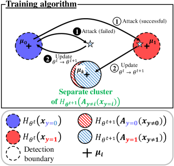
Figure 5: Training algorithm of our detector. The successful adversarial examples are re-labeled as $y=k$, and the failed adversarial examples are re-labeled as its original class before the attack. We update $\theta_{t}$ so that distances between representations and centers of their cluster are minimized.

Although we adaptively conduct attacks against $H_{\theta^{t}}$, the generated adversarial examples are not always successful. The successful attack is a case where the adaptive attack finds a perturbation $\mathbf{\delta}$ for $(\mathbf{x},y\texttt{=}i)\in\mathcal{D}$ so that $H_{\theta}(\mathbb{x}+\delta)$ gets inside of a detection boundary of other class $j\neq i$. In of Figure 5, it is illustrated that a successful adversarial example, whose original label is 0, crosses a detection boundary (dashed lines of circles) of class $y=1$ with perturbation $\delta$. On the other hand, a failed attack is a case where the adaptive attack can not find $\mathbf{\delta}$ such that $H_{\theta}(\mathbb{x}+\delta)$ does not get inside of decision boundaries of all other classes except the original label of $\mathbb{x}$. It is also illustrated as of Figure 5. The representation of failed adversarial example is not included in detection boundaries of any clusters $\mathbf{\mu}_{j\neq 0}$. We distinguish these two types of adversarial examples and deal with them in different ways in the following phase.

Phase 2. Re-labeling data and updating $\theta$.

After generating adversarial examples in the phase 1. We update parameter $\mathbf{\theta}^{t}$ to $\mathbf{\theta}^{t+1}$ with the adversarial examples and benign training data $\mathcal{D}$. We deal with those data with different re-labeling rules depending on representation clusters which the data should belong to. After the re-labeling, we get a new dataset $\mathcal{D}^{t}=\mathcal{D}_{S}^{t}\cup\mathcal{D}_{F}^{t}\cup\mathcal{D}$.

A. Re-labeling successful adversarial examples. We briefly explained successful adversarial examples in the description of the phase 1. They are adversarial examples which mislead our classification and bypass detection mechanism. It is strictly defined as $A_{S}(\mathcal{D})$,

$$A_{S}(\mathcal{D})=\{ A_{y=j}(\mathbf{x})|\;(\mathbf{x},i)\in\mathcal{D},$$ (20)

$$\exists j\neq i\;||H_{\theta^{t}}(A_{y=j}(\mathbf{x}))-\mathbf{\mu}_{j}||_{2}\leq\tau_{j}\}$$

To cluster the representations of $A_{S}(\mathcal{D})$ in a separate adversarial cluster ( of Figure 5), we define the dataset $\mathcal{D}^{t}_{S}$ by re-labeling $A_{S}(\mathcal{D})$ as $y=k$.

$$\mathcal{D}^{t}_{S}=\{(\mathbf{x},k)|\;\mathbf{x}\in A_{S}(\mathcal{D})\}$$ (21)

We set $\mathbf{\mu}_{k}$, a center of adversarial representations, to be an origin $\mathbf{0}_{m}$ in the representation space.

B. Re-labeling failed adversarial examples. Because an attack algorithm $A_{y=j}$ does not guarantee generation of $A_{S}(\mathcal{D})$, there exist adversarial examples which are perturbed with some $\mathbf{\delta}$ but failed to cross detection boundaries of other classes ( of Figure 5). We strictly define the failed adversarial examples as $A_{F}(\mathcal{D})$,

$$A_{F}(\mathcal{D})=\{ A_{y=j}(\mathbf{x})|\;(\mathbf{x},i)\in\mathcal{D},$$ (22)

$$\forall j\neq i\;||H_{\theta^{t}}(A_{y=j}(\mathbf{x}))-\mathbf{\mu}_{j}||_{2}>\tau_{j}\}$$

Since representations of the failed adversarial examples $A_{F}(\mathcal{D})$ neither are close to a cluster nor they form a cluster, re-labeling $A_{F}(\mathcal{D})$ to $k$ as like $A_{S}(\mathcal{D})$ has negative effects in clustering adversarial representations. Instead we re-label the failed adversarial example $A_{F}(\mathcal{D})$ to their original labels before the attack:

$$\begin{aligned} \mathcal{D}^{t}_{F}=\{(A_{y=j}&(\mathbf{x}),i)|\;(\mathbf{x},i)\in\mathcal{D},\\ &\exists j\neq i\;A_{y=j}(\mathbf{x})\in A_{F}(\mathcal{D})\}\end{aligned}$$ (23)

It is depicted in of Figure 5. By restricting changes of representations from small $\delta$ in input space, this re-labeling rule makes resulting $H_{\theta^{t+1}}$ more robust to input perturbations.

C. Updating model parameter $\mathbf{\theta}$. After the re-labeling process, we update parameter $\mathbf{\theta}^{t}$ to $\theta^{t+1}$ , as illustrated in and of Figure 5, to find distinct clusters of benign and adversarial representations. The updating process can be formalized as a likelihood maximization problem on the representations of $\mathcal{D}^{t}=\mathcal{D}_{S}^{t}\cup\mathcal{D}_{F}^{t}\cup\mathcal{D}$. The corresponding training objective can be expressed as follows,

$$\text{maximize}_{\theta}\mathcal{L}(\mathcal{D}^{t};\theta^{t})$$ (24)

$$\mathcal{L}(\mathcal{D}^{t};\theta^{t})=\sum_{(\mathbf{x},y)\in\mathcal{D}^{t}}p(H_{\theta^{t}}(\mathbf{x}))$$ (25)

We further expand Equation 25 under the GMM assumption in the model construction.

$$\begin{aligned} \mathcal{L}(\mathcal{D}^{t};\theta^{t})&=\sum_{(\mathbf{x},y)\in\mathcal{D}^{t}}p(H_{\theta^{t}}(\mathbf{x}))\\ &=\sum_{(\mathbf{x},y)\in\mathcal{D}^{t}}\sum_{i=0}^{k}p(y\texttt{=}i)p(H_{\theta^{t}}(\mathbf{x})|y\texttt{=}i)\\ &=\sum_{(\mathbf{x},y)\in\mathcal{D}^{t}}p(H_{\theta^{t}}(\mathbf{x})|y)\\ &=\sum_{(\mathbf{x},y)\in\mathcal{D}^{t}}N(z\texttt{=}H_{\theta^{t}}(\mathbf{x});\mu_{y},\mathbf{I}_{m})\\ &=\sum_{(\mathbf{x},y)\in\mathcal{D}^{t}}\mathcal{C}e^{-\frac{1}{2}||H_{\theta^{\prime}}(\mathbf{x})-\mu_{y}||^{2}_{2}}\end{aligned}$$ (26)

If we ignore the positive constant $\mathcal{C}$, we can regard this training objective minimizes distances between $H_{\theta^{t}}(\mathbf{x})$ and its target clustering center $\mu_{y}$. As we update $\theta^{t}$, $H_{\theta^{t+1}}$ better distinguishes the clusters of adversarial and benign representations.

However, in practice, we should resolve a problem where a ratio between the size of $\mathcal{D}^{t}_{S}$ and the size of $\mathcal{D}^{t}_{F}\cup\mathcal{D}$ is unbalanced. For example, if the size of $\mathcal{D}^{t}_{S}$ is 1 and the size of $\mathcal{D}^{t}_{F}\cup\mathcal{D}$ is 100, the effect of $\mathcal{D}^{t}_{S}$ to the total loss $\mathcal{L}(\mathcal{D}^{t};\theta^{t})$ is negligible, and $H_{\theta^{t+1}}$ hardly clusters the representations of $\mathcal{D}^{t}_{S}$. To fix this problem, we split $\mathcal{D}^{t}$ into $\mathcal{D}^{t}_{S}$ and $\mathcal{D}^{t}_{F}\cup\mathcal{D}$ , and compute the sum of average likelihoods of each dataset.

$$\begin{aligned} \mathcal{L}_{\text{fix}}(\mathcal{D}^{t};\theta^{t})=\frac{\mathcal{L}(\mathcal{D}_{S}^{t};\theta^{t})}{|\mathcal{D}_{S}^{t}|}+\frac{\mathcal{L}(\mathcal{D}_{F}^{t}\cup\mathcal{D};\theta^{t})}{|\mathcal{D}_{F}^{t}\cup\mathcal{D}|}\end{aligned}$$ (27)

Then we maximize $\mathcal{L}_{\text{fix}}(\mathcal{D}^{t};\theta^{t})$ instead of $\mathcal{L}(\mathcal{D}^{t};\theta^{t})$.

After we update the parameter to $\theta^{t+1}$, we go to the phase 1 and repeat this process until it converges enough, so the size of $\mathcal{D}^{t}_{S}$ is not decreasing more. Specifically we trained our models with the fixed number of epochs. We used 50 epochs for MNIST and 70 epochs for CIFAR10 with Adam optimizer [38] with a learning rate $10^{-3}$. We provide a pseudo code of stochastic mini-batch training in algorithm 1.

1:  $t\leftarrow 0$

2:  while $t<\rm{MAX\_EPOCHS}$ do

3:     $B\subset\mathcal{D}$ // $t^{\text{th}}$ benign mini batch.

4:     .// Phase 1. , of Figure 5

5:     $A_{S}(B)\leftarrow\{A_{y=j}(\mathbf{x})|\;(\mathbf{x},i)\in B,\linebreak{\color[rgb]{1,1,1}.}\;\;\;\;\;\;\;\;\;\;\;\;\;\;\;\;\;\;\;\exists j\neq i\;||H_{\theta^{t}}(A_{y=j}(\mathbf{x}))-\mathbf{\mu}_{j}||_{2}\leq\tau_{j}\}$

6:     $A_{F}(B)\leftarrow\{A_{y=j}(\mathbf{x})|\;(\mathbf{x},i)\in B,\linebreak{\color[rgb]{1,1,1}.}\;\;\;\;\;\;\;\;\;\;\;\;\;\;\;\;\;\;\;\forall j\neq i\;||H_{\theta^{t}}(A_{y=j}(\mathbf{x}))-\mathbf{\mu}_{j}||_{2}>\tau_{j}\}$

7:     .// Phase 2. , of Figure 5

8:     $B^{t}_{S}\leftarrow\{(\mathbf{x},k)|\mathbf{x}\in A_{S}(B)\}$

9:     $B^{t}_{F}\leftarrow\{(A_{y=j}(\mathbf{x}),i)|\;(\mathbf{x},i)\in\mathcal{D},\newline {\color[rgb]{1,1,1}.}\;\;\;\;\;\;\;\;\;\;\;\;\;\;\;\;\;\;\;\exists j\neq i\;A_{y=j}(\mathbf{x})\in A_{F}(\mathcal{D})\}$

10:     $B^{t}\leftarrow B_{S}^{t}\cup B_{F}^{t}\cup B$

11:     TRAIN $H_{\theta^{t}}$ to minimize $\mathcal{L}_{\text{fix}}(B^{t};\theta^{t})$

12:     $t\leftarrow t+1$

13:  end while

Algorithm 1 Training process of our adversarial detector.

4 Related Work

There is a broad range of literature in adversarial and robust learning, depending on objectives of attacks and defenses, or threat models [72]. Here we introduce and compare literature closely related to adversarial detection, and robust prediction.

4.1 Adversarial detectors

Adversarial detectors aim to detect adversarial examples before they compromise main tasks such as classifications. Depending on base mechanisms of the detectors, we can categorize them into three types.

Auxiliary discriminative detectors.

Early researchers introduced auxiliary discriminative detector model $p(y=\textit{adversarial}|x)$. It can be implemented as an additional class of adversarial examples in existing discriminative classifier [26, 1], or binary classification model [22, 54]. Then the detector is trained to discriminate adversarial examples from benign examples. However they are shown not effective against adaptive whitebox attacks where adversaries know everything about defenses and models [8]. We analyze this defect is from a limitation of discriminative approaches where they do not consider likelihood $p(\mathbf{x},y)$ (how likely $(\mathbf{x},y)$ exists). Even though $p(\mathbf{x},y)$ is very low, the discriminative approaches get to give high classification probability $p(y_{j}|\mathbf{x})=\frac{p(\mathbf{x},y_{j})}{\sum_{i}p(\mathbf{x},y_{i})}$, if $p(\mathbf{x},y_{j})$ of a class is relatively higher than $p(\mathbf{x},y_{i})$ of other classes. On the other hand, our approach directly estimates likelihoods of representations $p(\mathbf{z}\texttt{=}H_{\theta}(\mathbf{x}),y_{i})$ and does not suffer from the problem against adaptive whitebox attacks.

Likelihood or density based detectors.

Recent research introduced defenses based on generative models  [43, 45, 21, 63, 57, 59] or density estimation techniques [18, 37, 49] which aim to detect adversarial examples based on likelihoods. One type of them leverages distance metrics such as Mahalanobis distance in a representation space and detects adversarial examples if a distance between $\mathbf{x}$ and a cluster of benign data is larger than a threshold. However, as long as the overlaps of representations exist (as we found in motivational section 3.1), the distance metric can not be an effective method to detect adversarial examples. Its vulnerability is also studied by a prior work [66] showing that the Mahalanobis distance based detector [57] is still vulnerable in adaptive whitebox attack model. The other type of them [21, 59] leverages reconstruction loss of an input from encoder-decoder structures. It detects an input if the reconstruction loss of the input is larger than a predefined threshold. However reconstruction loss is not effective as input data become complex such as CIFAR10 and ImageNet. The vulnerability of this type of detector is studied in a prior [19]. In this paper, while the above approaches [43, 57] only focus on clusters of benign representations, we discover overlapping clusters of adversarial representations which reveals fundamental limitations of the distance based detectors. To resolve the problem we propose a new detector reducing the overlaps effectively detecting adversarial examples against adaptive whitebox attacks.

Statistical characteristics based detectors.

Besides the above approaches, many detectors are proposed suggesting new statistical characteristics of adversarial examples which can differentiate them from the benign examples [60, 53, 48, 73, 44]. For example a detector [73] computes classification probabilities of an input before and after applying input transformations. If the difference between the two probabilities is large, it regards the input as adversarial. The other detector [48] analyzes activation patterns (representations) of neurons of a classifier and compares the patterns to find different differences between benign and adversarial examples. However most of them are bypassed by adaptive whitebox attackers  [8, 30, 31]. Considering they rely on distance metrics on the representation space, we explain these failures are from the limitation of overlapping clusters of adversarial representations (section 3.1). In this paper we resolve this problem by reducing the overlaps between benign and adversarial representations.

4.2 Robust prediction

In contrast to the detectors, robust prediction methods try to classify adversarial examples to their true labels. We categorize them into three types according to their base approaches.

Adversarial training.

Adversarial training approaches [23, 51, 75] generate adversarial examples with attacks, such as FGSM and PGD, and augment them in training data. The augmented adversarial examples are re-labeled to their original labels so that they are correctly classified after the adversarial training. The adversarial training is empirically known as an effective robust prediction method which works against adaptive whitebox adversaries. They show robust classification accuracy regardless of types of attacks, if norms of perturbations $\delta$ are covered in the training process. On the other hand, the performances of adversarial training method significantly degrade if the perturbation $\delta$ is not covered. For example, a prior work [10] found adversarial training methods can be broken by unseen perturbations $\delta$ although $\ell_{1}$ of $\delta$ is small. On the other hand, our approach shows stable performances over various $\ell_{p}$ norm perturbations which implies the effectiveness of cluster separation (subsection 5.1).

Certified robust inferences.

To achieve guaranteed robustness against any attacks rather than empirical evidence, recent certified methods for robust inference rigorously prove there is no adversarial example with $\ell_{p}$ norm perturbations given inputs $\mathbf{x}$. They leverage several certification methods including satisfiability modulo theories [7, 17, 33, 36], mixed integer programming [6, 11, 16, 20, 47] , interval bound propagation [25, 76] , constraining Lipschitz constant of neural networks [2, 12, 24, 68] and randomized smoothing  [13, 41, 74, 61]. However those guarantees cost a lot of training or testing time for the verification, so many of them can not scale for practical applications of neural networks. Also some of certified methods [36, 12] degrade performances of neural networks constraining their robustness properties. Instead of taking the drawbacks of certifications, we propose a practical method for adversarial detection based on the cluster separation of adversarial representations.

Statistical defenses.

As like the statistical detectors, many robust prediction methods suggested statistical properties of adversarial examples [14, 71, 28, 62, 64, 62]. For instance, a defense method [14] learns which neurons of a model to be deactivated within a random process and improves the robustness of the model against a simple FGSM attack. Another defense method [71] also leverages randomness in input pre-processing including random re-sizing and random padding. But later they are turned out to be ineffective, just obfuscating gradients to disturb generations of adversarial examples. Attack methods such as backward pass differentiable approximation (BPDA) and expectation over transformations (EoT) are developed to break the obfuscated gradients [3]. In contrast, our approach does not rely on randomness or obfuscated gradients. We assure this by showing blackbox attacks do not outperform adaptive whitebox attacks (subsection 5.2) as suggested in the paper  [3].

4.3 Analysis of adversarial examples

Some of previous works studied root causes of adversarial attacks. It is suggested that recent neural networks are very linear and the linearity makes the networks very sensitive to small perturbations [23]. Meanwhile, assuming types of features, a dichotomy of robust feature and non-robust feature is proposed [67]. They analyze the intrinsic trade-off between robustness and accuracy. Interestingly in a following work [35], it is found that non-robust features suffice for achieving good accuracy on benign examples. In contrast the work defines vulnerable features as mathematical functions, we define adversarial examples as clusters of representations. Our definition enables us to assume separable clusters of adversarial representation, and further provide a robust detector effective against adaptive whitebox attacks.

5 Experiment

Table 1: Summary of baselines including our detector. For LID, MAHA, Madry and TRADES, we access codes provided by authors and use their pre-trained models for the evaluations. Others are re-implemented based on descriptions on papers. Resisting we used Convolutional VAE with 10 layers (MNIST) and 12 layers (CIFAR10). We use the same models provided by TRADES[75] for other approaches including ours.

	Detection metric / Detect if	Adaptive objective	Orignal source?	Benign clusters	Adversarial clusters	MNIST model	CIFAR10 model
Ours	(A) Distance to the closest representation cluster / High	Equation 7, $q(\mathbf{x})=||H_{\theta}(\mathbf{x})-\mu_{\hat{y}}||_{2}$	-	✓	✔	Small CNN	Wide Resnet
L-Ben (ablation)	(A) / High	Equation 7, $q(\mathbf{x})=||H_{\theta}(\mathbf{x})-\mu_{\hat{y}}||_{2}$	-	✓	-	Small CNN	Wide Resnet
Vanilla	(B) Classification probability / Low	Equation 3, Logit classification loss [9]	-	-	-	Small CNN	Wide Resnet
Resisting [21]	(A) + Reconstruction error / High	Equation 7, $q(\mathbf{x})=||H_{\theta}(\mathbf{x})-\mu_{\hat{y}}||_{2}+||\mathbf{x}-\textrm{rec}(\mathbf{x})||_{2}$	Re-implemented	✓	-	CNN_VAE (10L)	CNN_VAE(12L)
FS [73]	Classification difference after input processing /High	Equation 7, $q(\mathbf{x})=||H_{\theta}(\mathbf{x})-H_{\theta}(\mathbf{x^{\prime}})||_{1}$	Re-implemented	-	-	Small CNN	Wide Resnet
LID [49]	Local intrinsic dimensionality score / Low	Equation 7, $q(\mathbf{x})=$ LID-score($\mathbf{x}$)	Yes	✓	-	CNN (5L)	CNN (12L)
Madry [51]	(B) / Low	Equation 3, Logit classification loss [9]	Yes	-	-	CNN	w32-10 wide
TRADES [75]	(B) / Low	Equation 3, Logit classification loss [9]	Yes	-	-	Small CNN	Wide Resnet
MAHA [43]	(A), but Mahalanobis distance / High	Equation 7, $q(\mathbf{x})=$ Maha-score($\mathbf{x}$)	Yes	✓	-	-	Resnet  [43]

We conduct robust evaluations of our detector against both of adaptive whitebox attacks and blackbox attacks. With 4 perturbation types: $\ell_{p},p\in\{\infty,2,1,0\}$ and 7 types of attacks: PGD [51], MIM [15], CW [9], FGSM [23], Transfer [46], NES [34], Boundary [5], we empirically validate effectiveness of the reduced overlaps between adversarial and benign clusters of representations for adversarial detection. The attacks are implemented based on attacks publicly available from github repositories, Cleverhans and Foolbox . We implemented our detector model using PyTorch 1.6 [58] machine learning library. We mainly conducted our experiments on a server equipped with 4 of GTX 1080 Ti GPUs, an Intel i9-7900X processor and 64GB of RAM.

Baselines.

To demonstrate effectiveness of our detector, we compare our detector to 7 baselines summarized in Table 1. Ours is our detector trained to reduce overlaps between adversarial and benign clusters of representations. L-Ben is for an ablation study. It is an adversarial detector trained by re-labeling adversarial examples to the original labels (only conduct of Figure 5). Resisting [21] is a detector based on VAE [55]. It leverages a property that adversarial examples tend to have high reconstruction errors. It also leverages distances to the closest clusters as a detection metric. FS is a detector [73] which computes differences in classification probabilities before and after some input processing. We implemented the detector with median filters. LID and MAHA are detectors based on different distance metrics such as Local Intrinsic Dimensionality or Mahalanobis distances. These baselines show the limitation from the overlapping clusters of representations. Vanilla is a general discriminative classifier trained with cross entropy loss. Although vanilla is not applied any defense, we can leverage classification probabilities of Vanilla to detect adversarial examples [42]. Vanilla shows a lower bound of detection performances. Madry and TRADES are adversarial training methods which are not proposed as a detection method. However, they can be reformulated as detectors as Vanilla and we include them for comprehensive experiments between state-of-the-arts. Note that existing approaches do not deal with adversarial clusters.

Datasets.

We evaluate our detector models on two datasets, MNIST [40] and CIFAR10 [39]. MNIST contains grayscale hand-written digits from 0 to 9. This dataset is composed of a training set of 60,000 images and, a test set of 10,000 images with input dimension of 28$\times$28. CIFAR10 [39] contains 10 classes of real color images. This dataset is composed of a training set of 50,000 images, and a test set of 10,000 images with input dimension of 32$\times$32$\times$3. The values of data elements are scaled from 0.0 to 1.0. We selected the datasets since the datasets are representative benchmarks with which the baselines are tested.

Evaluation metric.

Performances of the baselines are computed in two evaluation metrics, Attack Success Ratio (ASR) and Expected ROC AUC scores (EROC). ASR evaluates practical defense performances of the baselines with a fixed detection threshold, while EROC reflects overall characteristics of detection metrics of the baselines.

ASR ranges from 0 to 1 and a lower value of ASR implies better detection performance. It is defined in the threat model section 2.3 and , in short, it is a success ratio of an attack over test inputs which are classified as true classes and not falsely detected as adversarial before the attack. Note that ASR can be different depending on how conservative a detection threshold is. For instance, if a detection threshold is chosen to have 50% of false positive ratio (50% of benign examples are falsely detected) it is much harder to bypass the detector and results in lower ASR value than when the threshold is chosen to have 1% of false positives. To reflect the above scenarios, we use suffix “-p” with ASR so that ASR-p means ASR when a detection threshold is chosen with p% of false positives.

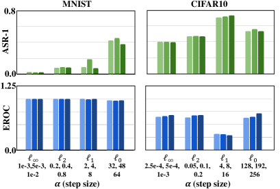
Figure 6: Robustness of Ours to attack parameter $\alpha$ (step size). Ours shows even or slight changes of detection performances. We select worst case $\alpha$ for the following experiments.

EROC ranges from 0 to 1 and a higher value of EROC implies better detection performances. EROC is proposed in this work as an extension of ROC AUC score [52]. ROC AUC score is a metric to evaluate how clearly a detector distinguishes positive samples and negative samples. However the metric is not compatible with our approach, because it only deals with detectors with a single detection metric. For example, our approach deal with one of $k$, the number of classes, detection metrics depending on the closest benign cluster given a representation (subsection 3.2). So we have $k$ ROC AUC scores, one for each class. To yield a single representative value, we get an expectation of the $k$ ROC AUC scores by a weighted summation of them. After an attack generates adversarial examples, a weight of ROC AUC score for class $i$ is computed as a fraction of the number of adversarial examples classified to class $i$ over the whole generated adversarial examples.

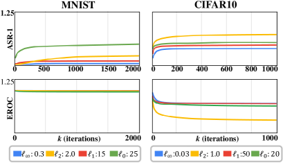
Figure 7: Robustness of Ours to attack parameter $k$ (iterations). The detection performances converge around $k=1000$ for all types of perturbation and we choose $k=1000$ for attacks in the remaining experiments.

5.1 Adaptive Whitebox Attack Test

Attack adaptation.

We evaluate the baselines against adaptive attacks, and the attacks are implemented based on PGD attack [51]. We summarize the adaptation methods for each baseline in the “Adaptive objective” column of Table 1. Basically adversaries adapt PGD attack by replacing $q(\mathbf{x})$ of Equation 7 with differentiable detection metric of a baseline. Depending on the detection conditions (“Detect if”), the sign of the $q(\mathbf{x})$ can be negated. For instance, an adversary can adapt PGD attack to Ours by replacing $q(\mathbf{x})$ of Equation 7 with Euclidean distance between $H_{\theta}(\mathbf{x})$ and to $\mathbf{\mu}_{i}$ of a wrong class $i$. For the case of Vanilla, Madry and TRADES, we used Logit classification loss [9] to deal with vanishing gradient problems from soft-max normalization layer of neural networks.

Table 2: Adaptive whitebox attacks test. Robustness of the baselines are evaluated against adaptive PGD attacks, and adversarial examples are generated with 4 types of perturbation. We can validate the effect of cluster separation of adversarial representations from the superior performances of Ours compared to L-Ben, Resisting, LID and MAHA which only consider clusters of benign representations. Although Madry and TRADES shows compatible performances on MNIST except PGD $\ell_{\infty}\texttt{=}0.4$, Ours outperforms them on CIFAR10 in regarding ASR-1.

MNIST										CIFAR10
		Ours	L-Ben	Vanilla	Resisting	FS	LID	Madry	TRADES			Ours	L-Ben	Vanilla	Resisting	FS	LID	Madry	TRADES	MAHA
	ACC.	0.97	0.97	0.99	0.99	0.97	0.98	0.98	0.99		ACC.	0.84	0.87	0.98	0.61	0.87	0.83	0.87	0.83	0.93
PGD $\ell_{\infty}\texttt{=}0.3$, T	ASR-1 $(\downarrow\downarrow)$	0.00	0.01	0.86	0.72	0.97	0.93	0.01	0.00	PGD $\ell_{\infty}\texttt{=}0.03$, T	ASR-1 $(\downarrow\downarrow)$	0.19	0.28	1.00	0.98	1.00	0.96	0.15	0.11	0.98
	EROC$(\uparrow\uparrow)$	1.00	1.00	0.98	0.95	0.36	0.62	1.00	1.00		EROC$(\uparrow\uparrow)$	0.91	0.82	0.45	0.00	0.03	0.47	0.98	0.98	0.06
PGD $\ell_{\infty}\texttt{=}0.3$, U	ASR-1 $(\downarrow\downarrow)$	0.01	0.06	0.86	0.89	1.00	0.98	0.03	0.01	PGD $\ell_{\infty}\texttt{=}0.03$, U	ASR-1 $(\downarrow\downarrow)$	0.40	0.55	1.00	0.99	1.00	1.00	0.44	0.40	1.00
	EROC$(\uparrow\uparrow)$	1.00	0.99	0.98	0.94	0.09	0.58	1.00	1.00		EROC$(\uparrow\uparrow)$	0.69	0.56	0.47	0.00	0.01	0.40	0.89	0.91	0.00
PGD $\ell_{\infty}\texttt{=}0.4$, T	ASR-1 $(\downarrow\downarrow)$	0.21	0.50	0.90	0.85	1.00	0.93	0.67	0.73	PGD $\ell_{\infty}\texttt{=}0.06$, T	ASR-1 $(\downarrow\downarrow)$	0.32	0.62	1.00	0.99	1.00	0.98	0.57	0.49	0.95
	EROC$(\uparrow\uparrow)$	0.99	0.97	0.98	0.93	0.10	0.63	0.87	0.89		EROC$(\uparrow\uparrow)$	0.76	0.46	0.45	0.00	0.00	0.46	0.79	0.88	0.37
PGD $\ell_{\infty}\texttt{=}0.4$, U	ASR-1 $(\downarrow\downarrow)$	0.51	0.85	0.85	0.95	1.00	0.98	0.94	0.95	PGD $\ell_{\infty}\texttt{=}0.06$, U	ASR-1 $(\downarrow\downarrow)$	0.61	0.89	1.00	0.99	1.00	1.00	0.80	0.82	1.00
	EROC$(\uparrow\uparrow)$	0.98	0.89	0.98	0.90	0.01	0.57	0.79	0.88		EROC$(\uparrow\uparrow)$	0.42	0.16	0.47	0.00	0.00	0.00	0.64	0.68	0.00
PGD $\ell_{2}\texttt{=}2.0$, T	ASR-1 $(\downarrow\downarrow)$	0.03	0.06	0.39	0.08	0.51	0.96	0.03	0.01	PGD $\ell_{2}\texttt{=}1.0$, T	ASR-1 $(\downarrow\downarrow)$	0.24	0.35	1.00	1.00	1.00	1.00	0.35	0.33	0.99
	EROC$(\uparrow\uparrow)$	1.00	0.99	0.98	1.00	0.89	0.59	1.00	1.00		EROC$(\uparrow\uparrow)$	0.89	0.78	0.40	0.02	0.01	0.47	0.91	0.94	0.02
PGD $\ell_{2}\texttt{=}2.0$, U	ASR-1 $(\downarrow\downarrow)$	0.09	0.21	0.75	0.27	0.88	1.00	0.14	0.07	PGD $\ell_{2}\texttt{=}1.0$, U	ASR-1 $(\downarrow\downarrow)$	0.48	0.60	1.00	1.00	1.00	1.00	0.67	0.74	1.00
	EROC$(\uparrow\uparrow)$	1.00	0.97	0.91	0.99	0.70	0.53	0.99	0.99		EROC$(\uparrow\uparrow)$	0.68	0.51	0.43	0.02	0.01	0.37	0.75	0.75	0.00
PGD $\ell_{1}\texttt{=}15$, T	ASR-1 $(\downarrow\downarrow)$	0.04	0.05	0.36	0.11	0.46	0.87	0.03	0.07	PGD $\ell_{1}\texttt{=}50$, T	ASR-1 $(\downarrow\downarrow)$	0.48	0.70	1.00	1.00	1.00	1.00	0.93	0.92	0.99
	EROC$(\uparrow\uparrow)$	1.00	0.99	0.99	1.00	0.91	0.61	1.00	1.00		EROC$(\uparrow\uparrow)$	0.67	0.42	0.31	0.00	0.00	0.45	0.37	0.47	0.02
PGD $\ell_{1}\texttt{=}15$, U	ASR-1 $(\downarrow\downarrow)$	0.19	0.11	0.73	0.37	0.84	0.98	0.11	0.09	PGD $\ell_{1}\texttt{=}50$, U	ASR-1 $(\downarrow\downarrow)$	0.72	0.94	1.00	1.00	1.00	1.00	0.98	0.99	1.00
	EROC$(\uparrow\uparrow)$	0.99	0.99	0.97	0.98	0.72	0.56	0.99	0.99		EROC$(\uparrow\uparrow)$	0.32	0.12	0.41	0.00	0.00	0.37	0.47	0.40	0.00
PGD $\ell_{0}\texttt{=}25$, T	ASR-1 $(\downarrow\downarrow)$	0.17	0.03	0.61	0.16	0.64	0.81	0.08	0.04	PGD $\ell_{0}\texttt{=}20$, T	ASR-1 $(\downarrow\downarrow)$	0.29	0.40	0.83	0.94	0.29	0.72	0.23	0.28	0.66
	EROC$(\uparrow\uparrow)$	0.99	0.99	0.93	0.99	0.85	0.65	0.99	1.00		EROC$(\uparrow\uparrow)$	0.88	0.82	0.71	0.00	0.95	0.52	0.96	0.95	0.78
PGD $\ell_{0}\texttt{=}25$, U	ASR-1 $(\downarrow\downarrow)$	0.45	0.12	0.85	0.68	0.93	0.98	0.23	0.19	PGD $\ell_{0}\texttt{=}20$, U	ASR-1 $(\downarrow\downarrow)$	0.53	0.60	0.98	0.98	0.52	0.92	0.53	0.64	0.76
	EROC$(\uparrow\uparrow)$	0.97	0.98	0.82	0.97	0.64	0.54	0.97	0.99		EROC$(\uparrow\uparrow)$	0.63	0.57	0.56	0.00	0.89	0.44	0.89	0.79	0.64
Worst case	ASR-1 $(\downarrow\downarrow)$	0.51	0.85	0.90	0.95	1.00	1.00	0.94	0.95	Worst case	ASR-1 $(\downarrow\downarrow)$	0.72	0.94	1.00	1.00	1.00	1.00	0.98	0.99	1.00
	EROC ($\uparrow\uparrow$)	0.97	0.89	0.82	0.90	0.01	0.53	0.79	0.88		EROC ($\uparrow\uparrow$)	0.32	0.12	0.31	0.00	0.00	0.00	0.37	0.40	0.00

Sensitiveness to attack parameters.

To demonstrate Ours is not sensitive to attack parameters, and to select strong attack parameters to evaluate robustness, we conduct two experiments. Specifically we test attack parameters $\alpha$ and $k$ in Equation 3. In the first experiment we test sensitiveness on $\alpha$ which is also called step size (Figure 6). We attacked Ours with the adaptive PGD attack varying $\alpha$ (x-axis). We could check Ours shows even or slight performance changes on both of the datasets (left and right) and metrics (top and bottom). In the following experiments, we conduct adaptive attacks with the several number of $\alpha$ (3 to 8) for all of the baselines and use the worst performances. In the second experiment, we analyze the strength of the attack parameter $k$, iterations. We increase $k$ from 0 to 2000 (MNIST) and from 0 to 1000 (CIFAR10), and plot the result in Figure 7. The ASR-1 and EROC for the both of the dataset converge before $k=1000$ (MNIST) and $k=800$ (CIFAR10), so we choose $k=1000$ as an attack iteration in the following experiments.

Robustness to various types of perturbation.

In Table 2, we evaluated the baselines under adaptive whitebox PGD attacks with various perturbation types $\ell_{p},p\in\{0,1,2,\infty\}$ for thorough comparisons of robustness between them. The left half of the table is for MNIST and the remaining half is for CIFAR10. On each half, the first column denotes types and sizes of perturbations, and whether an attack is targeted (T) or untargeted (U). For example, “PGD $\ell_{\infty}\texttt{=}0.3$, T” means the baselines are evaluated with adaptive PGD attack under perturbations $\delta$ whose $\ell_{\infty}$ norm are less than 0.3. For each of the attacks, we measure ASR-1 and EROC metrics. The down arrows of ASR-1 mean lower is better and the up arrows of EROC means higher is better. We stress the best performances with boldface. Note that we measure conservative ASR-1 which means detection thresholds with 1% of false positives.

Table 3: Blackbox attack test. Robustness of the baselines are evaluated against 3 different blackbox attacks with $\ell_{\infty}$ and $\ell_{2}$ perturbations. Most of the baselines are effective in the blackbox attack model.

MNIST										CIFAR10
		Ours	L-Ben	Vanilla	Resisting	FS	LID	Madry	TRADES			Ours	L-Ben	Vanilla	Resisting	FS	LID	Madry	TRADES	MAHA
Transfer $\ell_{\infty}\texttt{=}0.3$	ASR-1 $(\downarrow\downarrow)$	0.00	0.00	0.01	0.08	0.96	0.84	0.00	0.00	Transfer $\ell_{\infty}\texttt{=}0.03$	ASR-1 $(\downarrow\downarrow)$	0.02	0.00	0.71	0.15	0.55	0.52	0.01	0.01	0.78
	EROC$(\uparrow\uparrow)$	1.00	0.99	1.00	1.00	0.73	0.82	1.00	1.00		EROC$(\uparrow\uparrow)$	1.00	1.00	0.77	0.97	0.92	0.78	1.00	0.99	0.72
NES $\ell_{\infty}\texttt{=}0.3$	ASR-1 $(\downarrow\downarrow)$	0.01	0.05	0.69	0.54	0.75	0.92	0.03	0.01	NES $\ell_{\infty}\texttt{=}0.06$	ASR-1 $(\downarrow\downarrow)$	0.43	0.55	1.00	0.99	0.98	0.99	0.47	0.46	0.93
	EROC$(\uparrow\uparrow)$	1.00	0.99	0.76	0.98	0.66	0.69	1.00	1.00		EROC$(\uparrow\uparrow)$	0.71	0.59	0.02	0.00	0.35	0.69	0.88	0.88	0.11
NES $\ell_{2}\texttt{=}2.0$	ASR-1 $(\downarrow\downarrow)$	0.01	0.11	0.60	0.14	0.44	0.93	0.05	0.02	NES $\ell_{2}\texttt{=}1.0$	ASR-1 $(\downarrow\downarrow)$	0.37	0.40	1.00	0.99	0.95	0.98	0.55	0.57	0.65
	EROC$(\uparrow\uparrow)$	1.00	0.99	0.84	1.00	0.88	0.59	0.99	1.00		EROC$(\uparrow\uparrow)$	0.77	0.68	0.02	0.00	0.35	0.76	0.84	0.83	0.34
Boundary $\ell_{\infty}\texttt{=}0.3$	ASR-1 $(\downarrow\downarrow)$	0.00	0.00	0.00	0.00	0.54	0.89	0.00	0.00	Boundary $\ell_{\infty}\texttt{=}0.06$	ASR-1 $(\downarrow\downarrow)$	0.00	0.00	0.02	0.34	0.40	0.17	0.00	0.04	0.34
	EROC$(\uparrow\uparrow)$	1.00	1.00	1.00	1.00	0.96	0.75	1.00	1.00		EROC$(\uparrow\uparrow)$	1.00	1.00	1.00	0.95	0.93	0.90	1.00	0.98	0.92
Boundary $\ell_{2}\texttt{=}2.0$	ASR-1 $(\downarrow\downarrow)$	0.00	0.00	0.00	0.00	0.49	0.82	0.00	0.00	Boundary $\ell_{2}\texttt{=}1.0$	ASR-1 $(\downarrow\downarrow)$	0.02	0.00	0.01	0.14	0.43	0.06	0.00	0.05	0.38
	EROC$(\uparrow\uparrow)$	1.00	1.00	1.00	1.00	0.96	0.77	1.00	1.00		EROC$(\uparrow\uparrow)$	1.00	0.99	1.00	0.98	0.93	0.95	1.00	0.98	0.92

Table 4: Adaptive whitebox attack tests with different detection thresholds and attack methods.

MNIST						CIFAR10
		Ours	L-Ben	Vanilla	TRADES			Ours	L-Ben	Vanilla	TRADES
PGD $\ell_{\infty}\texttt{=}0.4$	ASR-2	0.32	0.69	0.56	0.89	PGD $\ell_{\infty}\texttt{=}0.06$	ASR-5	0.58	0.87	1.00	0.79
	ASR-5	0.09	0.48	0.01	0.59		ASR-10	0.56	0.86	1.00	0.72
	EROC	0.98	0.88	0.98	0.87		EROC	0.42	0.16	0.47	0.68
PGD $\ell_{2}\texttt{=}2.0$	ASR-2	0.05	0.17	0.58	0.04	PGD $\ell_{2}\texttt{=}1.0$	ASR-5	0.41	0.56	1.00	0.70
	ASR-5	0.02	0.09	0.19	0.02		ASR-10	0.34	0.52	1.00	0.63
	EROC	1.00	0.97	0.91	0.99		EROC	0.68	0.51	0.43	0.75
PGD $\ell_{0}\texttt{=}25$	ASR-2	0.36	0.10	0.68	0.14	PGD $\ell_{0}\texttt{=}20$	ASR-5	0.53	0.60	0.96	0.58
	ASR-5	0.19	0.04	0.26	0.08		ASR-10	0.48	0.52	0.92	0.49
	EROC	0.97	0.98	0.82	0.99		EROC	0.63	0.57	0.56	0.79
CW $\ell_{2}\texttt{=}2.0$	ASR-2	0.57	0.17	0.56	0.07	CW $\ell_{2}\texttt{=}1.0$	ASR-2	0.46	0.69	1.00	0.59
	ASR-5	0.43	0.11	0.53	0.03		ASR-5	0.37	0.66	1.00	0.54
	EROC	0.93	0.97	0.78	0.99		EROC	0.80	0.58	0.20	0.88
MIM $\ell_{\infty}\texttt{=}0.4$	ASR-2	0.49	0.62	0.76	0.71	MIM $\ell_{\infty}\texttt{=}0.06$	ASR-5	0.68	0.90	0.96	0.81
	ASR-5	0.23	0.42	0.41	0.47		ASR-10	0.66	0.89	0.93	0.79
	EROC	0.96	0.91	0.72	0.92		EROC	0.36	0.12	0.47	0.68
FGSM $\ell_{\infty}\texttt{=}0.4$	ASR-2	0.00	0.01	0.21	0.01	FGSM $\ell_{\infty}\texttt{=}0.06$	ASR-5	0.00	0.00	0.58	0.43
	ASR-5	0.00	0.00	0.13	0.00		ASR-10	0.00	0.00	0.40	0.35
	EROC	1.00	1.00	0.94	1.00		EROC	0.99	0.99	0.92	0.92
PGD $\ell_{\infty}\texttt{=}1.0$	ASR-2	1.00	1.00	0.56	0.95	PGD $\ell_{\infty}\texttt{=}1.0$	ASR-5	1.00	1.00	1.00	1.00
	ASR-5	0.99	1.00	0.01	0.81		ASR-10	1.00	1.00	0.99	1.00
	EROC	0.40	0.12	0.98	0.53		EROC	0.00	0.00	0.39	0.26
PGD $\ell_{2}\texttt{=}6.0$	ASR-2	0.94	0.90	0.66	0.89	PGD $\ell_{2}\texttt{=}6.0$	ASR-5	1.00	0.97	0.99	1.00
	ASR-5	0.85	0.75	0.26	0.72		ASR-10	1.00	0.95	0.98	1.00
	EROC	0.63	0.51	0.76	0.74		EROC	0.01	0.25	0.46	0.26

In the case of MNIST, Ours performs well across many types of perturbations with low ASR-1 and high EROC. Most of the ASR-1 are not higher than 0.20 and the lowest EROC is 0.97. Although Madry and TRADES are proposed as robust inference methods (subsection 4.2), they achieve good detection performances across the perturbation types. We regard it is because they are trained to lower classification probabilities (detection metric) of adversarial examples in their training process. However the performances of the robust inference methods show steep degradation up to ASR of 0.95 and EROC 0.79 if they are attacked with unseen size of perturbations (PGD $\ell_{\infty}\texttt{=}0.4$, U). In contrast, Ours shows less performance reduction (ASR-1 of 0.51 and EROC of 0.98). Compared to the L-Ben, which is for an ablation study to check effectiveness of separating clusters of adversarial representations, Ours performs superior to L-Ben for the all perturbation types except PGD $\ell_{0}\texttt{=}25$ and PGD $\ell_{1}\texttt{=}25$, U. This result validates the cluster separation between adversarial representations and benign representations reduces the overlaps between them and improves detection performances. As we observed in the motivational section (subsection 3.1), the detection method based on distances between representations (Resisting, LID, MAHA) does not show effective performances under adaptive whitebox attacks. In the case of CIFAR10, we observe consistent results with MNIST dataset. The robust inference methods (Madry, TRADES) achieved good detection metrics across the perturbation types while showing large degradation in the case of unseen size of perturbations (PGD, $\ell_{\infty}\texttt{=}0.06$, U). The ablation study between Ours and L-ben still holds in CIFAR10, even improving performances on the perturbation types $\ell_{0}$ and $\ell_{1}$.

In summary, Ours achieves improves worst case ASR-1 by 45% (MNIST) and 27% (CIFAR10) over the existing adversarial detectors and robust inference methods. We also validate our argument about separation of adversarial clusters in a representation space is effective with the comparisons to L-ben and three representation-distance based detectors (Resisting, LID, MAHA).

Robustness to thresholds and attack methods.

We analyze the detectors more closely with different detection thresholds and against different attack methods. We previously analyzed the performances of the baseline detectors with very low 1% false positives thresholds to conservatively compare them. However the conservative analysis has a limitation that it can not evaluate how well a detection approach reduces ASR as increasing the threshold. So we compare the ASR reduction property varying the thresholds in Table 4. We only demonstrate a subset of the baselines for compact comparisons. First of all, we analyze the baselines under attacks where they show relatively high ASR-1 compared to the other attacks in Table 2. They correspond to the first three rows of attacks in Table 4. Note that we conduct all attacks in untargeted way and measured two ASR with different thresholds. In case of MNIST, under the PGD $\ell_{\infty}\texttt{=}0.4$, Ours shows 0.09 of ASR-5 which is much lower than 0.59 of TRADES. Vanilla reduces to 0.01 of ASR while does not reduce ASR on CIFAR10.

Next, we evaluate the baselines against different attack methods. The methods include Carlini & Wager (CW) [8], Momentum Iterative Method (MIM) [15] and Fast Gradient Sign Method (FGSM) [23] and we adapt them to each baseline. The second three rows of Table 4 show the results of the attacks. We conduct CW attack finding the best confidence parameters with 5 binary searches. For the MIM attack we use momentum decay factor with 0.9. We find CW attack is more powerful than PGD attack to Ours, showing higher ASR on MNIST. However Ours still retains EROC of 0.93 which shows its effectiveness. On the other hand, Ours achieves the best ASR-2 and ASR-5 score against CW attacks on CIFAR10. Against MIM $\ell_{\infty}$, we can check consistent results with PGD $\ell_{\infty}$ showing a little performance degradation from all baselines. Under FGSM $\ell_{\infty}$, which performs a single step perturbation, all baselines perform well except TRADES shows High ASR-5 and low EROC.

In addition to the above evaluations, we attack the baselines with large perturbations $\ell_{\infty}\texttt{=}1.0$ and $\ell_{2}\texttt{=}6.0$ for validating Ours does not depend on obfuscated gradients , as suggested in a prior work  [3]. We checked ASRs of Ours reach near 1.00 under the large perturbation attacks which confirm obfuscated gradient problem does not occur in case of Ours.

5.2 Blackbox Attack Test

We evaluate the defenses under three blackbox attacks in Table 3 and the details of the attacks are explained in subsection 2.2. This experiment provides another evidence that Ours does not exploit obfuscated gradients [3]. Overall, most of the baselines performs well against the blackbox attacks while FS and LID are not effective. In the case of FS, median filter alone is not enough detection mechanism [73, 30] even though the attack is not adapted to FS (Transfer). LID is suggested to be used with an auxiliary discriminative detector, however the detection score alone can not discriminate adversarial examples from benign examples. We validate there is no obfuscated gradients problem, verifying no blackbox attacks perform better than adaptive whitebox attacks.

6 Conclusion

In this work, we introduced a new adversarial detector under the novel hypothesis of separable clusters of adversarial representations and we proposed to learn the separable clusters formulating an optimization problem of deep neural networks. Specifically, we modeled the representation space as a mixture of Gaussians. We validated our model under both of the adaptive whitebox attacks and blackbox attacks. Studying more effective assumptions on the distribution of representations and applying our defense to different tasks would be interesting future research.

References

- [1] Mahdieh Abbasi, Arezoo Rajabi, Azadeh Sadat Mozafari, Rakesh B. Bobba, and Christian Gagne. Controlling over-generalization and its effect on adversarial examples generation and detection. 2018.
- [2] Cem Anil, James Lucas, and Roger Grosse. Sorting out lipschitz function approximation. In International Conference on Machine Learning, pages 291–301, 2019.
- [3] Anish Athalye, Nicholas Carlini, and David Wagner. Obfuscated Gradients Give a False Sense of Security : Circumventing Defenses to Adversarial Examples. In In Proceedings of the 35th International Conference on Machine Learning, 2018.
- [4] Battista Biggio, Igino Corona, Davide Maiorca, Blaine Nelson, Nedim Šrndić, Pavel Laskov, Giorgio Giacinto, and Fabio Roli. Evasion attacks against machine learning at test time. In Joint European conference on machine learning and knowledge discovery in databases, pages 387–402. Springer, 2013.
- [5] Wieland Brendel, Jonas Rauber, and Matthias Bethge. Decision-based adversarial attacks: Reliable attacks against black-box machine learning models, 2017.
- [6] Rudy R Bunel, Ilker Turkaslan, Philip Torr, Pushmeet Kohli, and Pawan K Mudigonda. A unified view of piecewise linear neural network verification. In Advances in Neural Information Processing Systems, pages 4790–4799, 2018.
- [7] Nicholas Carlini, Guy Katz, Clark Barrett, and David L. Dill. Provably minimally-distorted adversarial examples, 2018.
- [8] Nicholas Carlini and David Wagner. Adversarial Examples Are Not Easily Detected : Bypassing Ten Detection Methods. In In Proceedings of the 10th ACM Workshop on Artificial Intelligence and Security, 2017.
- [9] Nicholas Carlini and David Wagner. Towards Evaluating the Robustness of Neural Networks. In IEEE Symposium on Security and Privacy, 2017.
- [10] Pin-Yu Chen, Yash Sharma, Huan Zhang, Jinfeng Yi, and Cho-Jui Hsieh. EAD: Elastic-Net Attacks to Deep Neural Networks via Adversarial Examples. In In AAAI Conference on Artificial Intelligence, 2018.
- [11] Chih-Hong Cheng, Georg Nührenberg, and Harald Ruess. Maximum resilience of artificial neural networks. In International Symposium on Automated Technology for Verification and Analysis, pages 251–268. Springer, 2017.
- [12] Moustapha Cisse, Piotr Bojanowski, Edouard Grave, Yann Dauphin, and Nicolas Usunier. Parseval networks: Improving robustness to adversarial examples. arXiv preprint arXiv:1704.08847, 2017.
- [13] Jeremy M Cohen, Elan Rosenfeld, and J Zico Kolter. Certified adversarial robustness via randomized smoothing. In Proceedings of the 36th International Conference on Machine Learning (ICML 2019), 2019.
- [14] Guneet S Dhillon, Kamyar Azizzadenesheli, and Zachary C Lipton. Towards the first adversarially robust neural network model on mnist. In International Conference on Learning Representations (ICLR), 2018.
- [15] Yinpeng Dong, Fangzhou Liao, Tianyu Pang, Hang Su, Jun Zhu, Xiaolin Hu, and Jianguo Li. Boosting Adversarial Attacks with Momentum. In In Proceedings of the IEEE Conference on Computer Vision and Pattern Recognition (CVPR), 2018.
- [16] Souradeep Dutta, Susmit Jha, Sriram Sanakaranarayanan, and Ashish Tiwari. Output range analysis for deep neural networks. arXiv preprint arXiv:1709.09130, 2017.
- [17] Ruediger Ehlers. Formal verification of piece-wise linear feed-forward neural networks. In International Symposium on Automated Technology for Verification and Analysis, pages 269–286. Springer, 2017.
- [18] Reuben Feinman, Ryan R Curtin, Saurabh Shintre, and Andrew B Gardner. Detecting Adversarial Samples from Artifacts. 2017.
- [19] Ethan Fetaya, Joern-Henrik Jacobsen, Will Grathwohl, and Richard Zemel. Understanding the limitations of conditional generative models. In International Conference on Learning Representations, 2020.
- [20] Matteo Fischetti and Jason Jo. Deep neural networks and mixed integer linear optimization. Constraints, 23(3):296–309, 2018.
- [21] Partha Ghosh, Arpan Losalka, and Michael J. Black. Resisting adversarial attacks using gaussian mixture variational autoencoders. Proceedings of the AAAI Conference on Artificial Intelligence, 33:541–548, Jul 2019.
- [22] Zhitao Gong, Wenlu Wang, and Wei-shinn Ku. Adversarial and Clean Data Are Not Twins. 2017.
- [23] Ian J Goodfellow, Jonathon Shlens, and Christian Szegedy. Explaining and harnessing adversarial examples. In International Conference on Learning Representations (ICLR), 2015.
- [24] Henry Gouk, Eibe Frank, Bernhard Pfahringer, and Michael Cree. Regularisation of neural networks by enforcing lipschitz continuity. arXiv preprint arXiv:1804.04368, 2018.
- [25] Sven Gowal, Krishnamurthy Dvijotham, Robert Stanforth, Rudy Bunel, Chongli Qin, Jonathan Uesato, Relja Arandjelovic, Timothy Mann, and Pushmeet Kohli. On the effectiveness of interval bound propagation for training verifiably robust models. arXiv preprint arXiv:1810.12715, 2018.
- [26] Kathrin Grosse, Praveen Manoharan, Nicolas Papernot, Michael Backes, and Patrick Mcdaniel. On the ( Statistical ) Detection of Adversarial Examples. 2017.
- [27] Shixiang Gu and Luca Rigazio. Towards deep neural network architectures robust to adversarial examples. In International Conference on Learning Representations (ICLR) Workshops, 2015.
- [28] Chuan Guo, Mayank Rana, Moustapha Cisse, and Laurens Van Der Maaten. Countering adversarial images using input transformations. arXiv preprint arXiv:1711.00117, 2017.
- [29] Kaiming He, Xiangyu Zhang, Shaoqing Ren, and Jian Sun. Deep residual learning for image recognition. In Proceedings of the IEEE conference on computer vision and pattern recognition, pages 770–778, 2016.
- [30] Warren He, James Wei, Xinyun Chen, Nicholas Carlini, and Dawn Song. Adversarial example defense: Ensembles of weak defenses are not strong. In 11th USENIX Workshop on Offensive Technologies (WOOT 17), 2017.
- [31] Hossein Hosseini, Sreeram Kannan, and Radha Poovendran. Are odds really odd? bypassing statistical detection of adversarial examples. In Proceedings of the 35th International Conference on Machine Learning, ICML 2018, 2018.
- [32] Gao Huang, Zhuang Liu, Laurens Van Der Maaten, and Kilian Q Weinberger. Densely connected convolutional networks. In Proceedings of the IEEE conference on computer vision and pattern recognition, pages 4700–4708, 2017.
- [33] Xiaowei Huang, Marta Kwiatkowska, Sen Wang, and Min Wu. Safety verification of deep neural networks. In International Conference on Computer Aided Verification, pages 3–29. Springer, 2017.
- [34] Andrew Ilyas, Logan Engstrom, Anish Athalye, and Jessy Lin. Black-box adversarial attacks with limited queries and information. In Proceedings of the 35th International Conference on Machine Learning, ICML 2018, July 2018.
- [35] Andrew Ilyas, Shibani Santurkar, Dimitris Tsipras, Logan Engstrom, Brandon Tran, and Aleksander Madry. Adversarial examples are not bugs, they are features. In Conference on Neural Information Processing Systems (NeurIPS), 2019.
- [36] Guy Katz, Clark W. Barrett, David L. Dill, Kyle Julian, and Mykel J. Kochenderfer. Reluplex: An efficient SMT solver for verifying deep neural networks. CoRR, abs/1702.01135, 2017.
- [37] Jinhan Kim, Robert Feldt, and Shin Yoo. Guiding deep learning system testing using surprise adequacy. In Proceedings of the 41st International Conference on Software Engineering, ICSE ’19, page 1039–1049. IEEE Press, 2019.
- [38] Diederik P Kingma and Jimmy Ba. Adam: A method for stochastic optimization. arXiv preprint arXiv:1412.6980, 2014.
- [39] Alex Krizhevsky. Learning multiple layers of features from tiny images. page 541–548, Jul 2009.
- [40] Yann LeCun, Léon Bottou, Yoshua Bengio, and Patrick Haffner. Gradient-based learning applied to document recognition. In Proceedings of the IEEE, 86(11):2278–2324, 1998.
- [41] Mathias Lecuyer, Vaggelis Atlidakis, Roxana Geambasu, Daniel Hsu, and Suman Jana. Certified robustness to adversarial examples with differential privacy. In 2019 IEEE Symposium on Security and Privacy (SP), pages 656–672. IEEE, 2019.
- [42] Kimin Lee, Honglak Lee, Kibok Lee, and Jinwoo Shin. Training confidence-calibrated classifiers for detecting out-of-distribution samples. arXiv preprint arXiv:1711.09325, 2017.
- [43] Kimin Lee, Kibok Lee, Honglak Lee, and Jinwoo Shin. A simple unified framework for detecting out-of-distribution samples and adversarial attacks. In Conference on Neural Information Processing Systems (NIPS), 2018.
- [44] Xin Li and Fuxin Li. Adversarial examples detection in deep networks with convolutional filter statistics. 2017 IEEE International Conference on Computer Vision (ICCV), Oct 2017.
- [45] Yingzhen Li, John Bradshaw, and Yash Sharma. Are generative classifiers more robust to adversarial attacks? In Proceedings of the 35th International Conference on Machine Learning, volume abs/1802.06552, 2018.
- [46] Yanpei Liu, Xinyun Chen, Chang Liu, and Dawn Song. Delving into transferable adversarial examples and black-box attacks. In International Conference on Learning Representations (ICLR), 2017.
- [47] Alessio Lomuscio and Lalit Maganti. An approach to reachability analysis for feed-forward relu neural networks. arXiv preprint arXiv:1706.07351, 2017.
- [48] Shiqing Ma, Yingqi Liu, Guanhong Tao, Wen-chuan Lee, and Xiangyu Zhang. NIC : Detecting Adversarial Samples with Neural Network Invariant Checking. In Proceedings of the 2019 Annual Network and Distributed System Security Symposium (NDSS), 2019.
- [49] Xingjun Ma, Bo Li, Yisen Wang, Sarah M. Erfani, Sudanthi Wijewickrema, Grant Schoenebeck, Dawn Song, Michael E. Houle, and James Bailey. Characterizing adversarial subspaces using local intrinsic dimensionality, 2018.
- [50] Laurens van der Maaten and Geoffrey Hinton. Visualizing data using t-sne. Journal of machine learning research, 9(Nov):2579–2605, 2008.
- [51] Aleksander Ma̧dry, Aleksandar Makelov, Ludwig Schmidt, Dimitris Tsipras, and Adrian Vladu. Towards Deep Learning Models Resistant to Adversarial Attacks. In International Conference on Learning Representations (ICLR), 2018.
- [52] Donna Katzman McClish. Analyzing a portion of the roc curve. Medical Decision Making, 9(3):190–195, 1989.
- [53] Dongyu Meng and Hao Chen. Magnet. Proceedings of the 2017 ACM SIGSAC Conference on Computer and Communications Security - CCS ’17, 2017.
- [54] JH Metzen, T Genewein, V Fischer, and B Bischoff. On detecting adversarial perturbations. 2017.
- [55] Diederik P. Kingma and Max Welling. Auto-Encoding Variational Bayes. In International Conference on Learning Representations (ICLR), 2013.
- [56] Tianyu Pang, Chao Du, Yinpeng Dong, and Jun Zhu. Towards Robust Detection of Adversarial Examples. In Conference on Neural Information Processing Systems (NIPS), 2018.
- [57] Tianyu Pang, Kun Xu, Yinpeng Dong, Chao Du, Ning Chen, and Jun Zhu. Rethinking softmax cross-entropy loss for adversarial robustness. In International Conference on Learning Representations, 2020.
- [58] Adam Paszke, Sam Gross, Francisco Massa, Adam Lerer, James Bradbury, Gregory Chanan, Trevor Killeen, Zeming Lin, Natalia Gimelshein, Luca Antiga, et al. Pytorch: An imperative style, high-performance deep learning library. In Advances in neural information processing systems, pages 8026–8037, 2019.
- [59] Yao Qin, Nicholas Frosst, Sara Sabour, Colin Raffel, Garrison Cottrell, and Geoffrey Hinton. Detecting and diagnosing adversarial images with class-conditional capsule reconstructions. In International Conference on Learning Representations, 2020.
- [60] Kevin Roth, Yannic Kilcher, and Thomas Hofmann. The odds are odd: A statistical test for detecting adversarial examples. arXiv preprint arXiv:1902.04818, 2019.
- [61] Hadi Salman, Jerry Li, Ilya Razenshteyn, Pengchuan Zhang, Huan Zhang, Sebastien Bubeck, and Greg Yang. Provably robust deep learning via adversarially trained smoothed classifiers. In Advances in Neural Information Processing Systems, pages 11292–11303, 2019.
- [62] Pouya Samangouei, Maya Kabkab, and Rama Chellappa. Defense-gan: Protecting classifiers against adversarial attacks using generative models. In International Conference on Learning Representations (ICLR), 2018.
- [63] Lukas Schott, Jonas Rauber, Matthias Bethge, and Wieland Brendel. Towards the first adversarially robust neural network model on mnist. In International Conference on Learning Representations (ICLR), 2019.
- [64] Yang Song, Taesup Kim, Sebastian Nowozin, Stefano Ermon, and Nate Kushman. Pixeldefend: Leveraging generative models to understand and defend against adversarial examples. In International Conference on Learning Representations, 2018.
- [65] Christian Szegedy, Joan Bruna, Dumitru Erhan, and Ian Goodfellow. Intriguing properties of neural networks. In In International Conference on Learning Representations (ICLR), 2014.
- [66] Florian Tramer, Nicholas Carlini, Wieland Brendel, and Aleksander Madry. On adaptive attacks to adversarial example defenses, 2020.
- [67] Dimitris Tsipras, Shibani Santurkar, Logan Engstrom, Alexander Turner, and Aleksander Ma̧dry. Robustness May Be at Odds with Accuracy. In International Conference on Learning Representations (ICLR), 2018.
- [68] Yusuke Tsuzuku, Issei Sato, and Masashi Sugiyama. Lipschitz-margin training: Scalable certification of perturbation invariance for deep neural networks. In Advances in neural information processing systems, pages 6541–6550, 2018.
- [69] Jingyi Wang, Guoliang Dong, Jun Sun, Xinyu Wang, and Peixin Zhang. Adversarial Sample Detection for Deep Neural Network through Model Mutation Testing. In CoRR, 2018.
- [70] Daan Wierstra, Tom Schaul, Jan Peters, and Juergen Schmidhuber. Natural evolution strategies. In 2008 IEEE Congress on Evolutionary Computation (IEEE World Congress on Computational Intelligence), pages 3381–3387. IEEE, 2008.
- [71] Cihang Xie, Jianyu Wang, Zhishuai Zhang, Zhou Ren, and Alan Yuille. Mitigating adversarial effects through randomization. arXiv preprint arXiv:1711.01991, 2017.
- [72] Han Xu, Yao Ma, Hao-Chen Liu, Debayan Deb, Hui Liu, Ji-Liang Tang, and Anil K. Jain. Adversarial attacks and defenses in images, graphs and text: A review. International Journal of Automation and Computing, 17(2):151–178, Mar 2020.
- [73] Weilin Xu, David Evans, and Yanjun Qi. Feature Squeezing : Detecting Adversarial Examples in Deep Neural Networks. In Proceedings of the 2018 Annual Network and Distributed System Security Symposium (NDSS), 2018.
- [74] Runtian Zhai, Chen Dan, Di He, Huan Zhang, Boqing Gong, Pradeep Ravikumar, Cho-Jui Hsieh, and Liwei Wang. Macer: Attack-free and scalable robust training via maximizing certified radius. In International Conference on Learning Representations, 2020.
- [75] Hongyang Zhang, Yaodong Yu, Jiantao Jiao, Eric P Xing, Laurent El Ghaoui, and Michael I Jordan. Theoretically principled trade-off between robustness and accuracy. In Proceedings of the 36th International Conference on Machine Learning (ICML 2019), 2019.
- [76] Huan Zhang, Hongge Chen, Chaowei Xiao, Sven Gowal, Robert Stanforth, Bo Li, Duane Boning, and Cho-Jui Hsieh. Towards stable and efficient training of verifiably robust neural networks. In In International Conference on Learning Representations (ICLR), 2020.
- [77] Stephan Zheng, Yang Song, Thomas Leung, and Ian Goodfellow. Improving the robustness of deep neural networks via stability training. In In The IEEE Conference on Computer Vision and Pattern Recognition (CVPR), 2016.