Rethinking Learnable Tree Filter for
Generic Feature Transform

Abstract

The Learnable Tree Filter presents a remarkable approach to model structure-preserving relations for semantic segmentation. Nevertheless, the intrinsic geometric constraint forces it to focus on the regions with close spatial distance, hindering the effective long-range interactions. To relax the geometric constraint, we give the analysis by reformulating it as a Markov Random Field and introduce a learnable unary term. Besides, we propose a learnable spanning tree algorithm to replace the original non-differentiable one, which further improves the flexibility and robustness. With the above improvements, our method can better capture long-range dependencies and preserve structural details with linear complexity, which is extended to several vision tasks for more generic feature transform. Extensive experiments on object detection/instance segmentation demonstrate the consistent improvements over the original version. For semantic segmentation, we achieve leading performance (82.1% mIoU) on the Cityscapes benchmark without bells-and-whistles. Code is available at https://github.com/StevenGrove/LearnableTreeFilterV2.

1 Introduction

In the last decade, the vision community has witnessed the extraordinary success of deep convolutional networks in various vision tasks [1, 2, 3, 4, 5, 6, 7, 8]. However, in deep convolutional layers, the distribution of impact within an effective receptive field is found to be limited to a local region and converged to the gaussian [9], which brings difficulties to the long-range dependencies modeling. To address this problem, numerous local-based approaches [10, 11, 12] have been proposed to increase the receptive region of convolutional kernels by using pooling [13] or dilated operations [14]. Meanwhile, various global-based approaches [15, 16, 17, 18, 19] have been explored to aggregate features by modeling the pairwise relations based on the visual attention mechanism. However, there is still a conflict between long-range dependencies modeling and object details preserving.

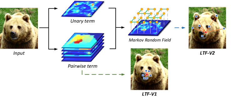
Figure 1: The comparison of the aggregation processes between the LTF-V1 module [20] and the proposed LTF-V2 module. One of the sink nodes is marked by the red square, and the corresponding source nodes with the highest filtering weights are presented as the blue squares. Limited by the intrinsic geometric constraint, the LTF-V1 can only give priority to the regions with close spatial distance. Different from it, our proposed LTF-V2 is more generic by adding a learnable unary term, which relaxes the geometric constraint and allows the filter to focus on the distant regions of interest.

Recently, the learnable tree filter module [20] (LTF-V1 module) tries to bridge this gap by performing feature aggregation on a minimum spanning tree. Since the minimum spanning tree is generated by the low-level guided features, it can retain the structural details with efficiency. Nevertheless, the geometric constraint and the construction process in the LTF-V1 module are found to be its Achilles’ heels, which impede the usage for more generic feature transform. Firstly, the interactions with distant nodes along the spanning tree need to pass through nearby nodes, which brings the intrinsic geometric constraint to the tree filter. As illustrated in Fig. 1, this property forces the LTF-V1 module to focus on the nearby regions. In addition, the construction process of the minimum spanning tree is non-differentiable, which is overly sensitive to the quality of guided features and prevents the LTF-V1 module from entirely learnable.

To remedy the shortages mentioned above, we rethink the learnable tree filter from the perspective of Markov Random Field [21] (MRF) and present the Learnable Tree Filter V2 Module (LTF-V2 module) for more generic feature transform. Specifically, it complements the LTF-V1 module by introducing a learnable unary term and a learnable spanning tree algorithm. The former one provides a modulation scalar [22, 23, 24] for each node, which can relax the geometric constraint and enable effective long-range interactions. Intuitively, as shown in the Fig. 1, the proposed unary term guides the LTF-V2 to focus on the coarsely distant regions of interest, and the tree-based pairwise term further refines the regions to fit original structures, bringing powerful semantic representations. Meanwhile, the proposed learnable spanning tree algorithm offers a simple and effective strategy to create a gradient tunnel between the spanning tree process and the feature transform module. This algorithm enables the LTF-V2 module to be more robust and flexible. Moreover, the LTF-V2 module maintains linear computational complexity and highly empirical efficiency of the LTF-V1 .

Overall, in this paper, we present a more generic method for structure-preserving feature transform with linear complexity. To demonstrate the effectiveness of the LTF-V2 module, we conduct extensive ablation studies on object detection, instance segmentation, and semantic segmentation. Both quantitative and qualitative experiments demonstrate the superiority of the LTF-V2 module over previous approaches. Even compared with other state-of-the-art works, the LTF-V2 module achieves competitive performance with much less resource consumption. Specifically, when applied to Mask R-CNN [25] (with ResNet50-FPN [26]), the LTF-V2 module obtains 2.4% and 1.8% absolute gains over the baseline on COCO benchmark for $\rm{AP}^{box}$ and $\rm{AP}^{seg}$ respectively, with negligible computational overhead. Meanwhile, the LTF-V2 module achieves 82.1% mIoU on Cityscapes benchmark without bells-and-whistles, reaching leading performance on semantic segmentation.

2 Related Work

Since each neuron has limited effective receptive field, the deep convolutional networks [1, 3, 26] typically fail to capture long-range dependencies. Recently, to alleviate the problem, a large number of approaches have been proposed to model long-range context in existing deep convolutional models. These approaches can be generally divided into two categories, namely local-based and global-based.

The local-based approaches aim to aggregate the long-range context by increasing the local receptive region of each neuron, e.g., pooling operation and dilated convolution. He et al. [27] and Zhao et al. [13] propose a spatial pyramid pooling for object detection and semantic segmentation, respectively. Yu et al. [28] introduces the dilated convolution to enlarge the receptive field of each convolution kernel explicitly. Dai et al. [12] further modifies the dilated convolution to a more generic form by replacing the grid kernels with the deformable ones. However, the modeling of pairwise relation by these methods is typically restricted to a local region and relies on the homogeneous prior.

The global-based approaches are mainly based on the attention mechanism, which is firstly applied in machine translation [29] as well as physical system modeling [30] and then extended to various vision tasks [15]. SENet [31], PSANet [32], and GENet [33] bring channel-wise relations to the network by performing down-sampling and attention in different channels. Non-Local [15] adopts the self-attention mechanism in the spatial domain to aggregate related features by generating the affinity matrix between each spatial node. It can model non-local relations but suffers from highly computational complexity. LatentGNN [18] and CCNet [16] are proposed to alleviate this problem by projecting features into latent space and stacking two criss-cross blocks, respectively.

Nevertheless, with the expansive receptive field, the detailed structure could not be preserved in the above methods. Our method bridges this gap by taking advantages of structure-aware spanning trees and global modeling of Markov Random Field.

3 Method

In this section, we theoretically analyze the deficiency of the LTF-V1 by reformulating it as a Markov Random Field and give a solution, namely the LTF-V2. Besides, we propose a learnable spanning tree algorithm to improve robustness and flexibility. With these improvements, we further present a new learnable tree filter module, called LTF-V2 module.

3.1 Notation and Problem Definition

Given an input feature map ${X}=\{x_{i}\}^{N}$ with $x_{i}\in\mathbb{R}^{1\times C}$ and the corresponding guidance ${G}=\{g_{i}\}^{N}$ with $g_{i}\in\mathbb{R}^{1\times C}$, where $N$ and $C$ indicate the number of input pixels and encoding channels, respectively. Specifically, the guidance ${G}$ gives the positions where the filter needs to preserve detailed structures. Following the original configuration [34, 20], we represent the topology of the guidance ${G}$ as a 4-connected planar graph, i.e., $\mathcal{G}=\{\mathcal{V},\mathcal{E}\}$, where $\mathcal{V}=\{\mathcal{V}_{i}\}^{N}$ is the set of nodes and $\mathcal{E}=\{\mathcal{E}_{i}\}^{N}$ is the set of edges. The weight of the edge reflects the feature distance between adjacent nodes. Our goal is to obtain the refined feature map ${Y}$ by transforming the input feature map ${X}$ with the property of guided graph $\mathcal{G}$, where the dimension of ${Y}$ is same with that of ${X}$.

3.2 Revisiting the Learnable Tree Filter V1

Recently, a learnable tree filter module [20] (LTF-V1 module) has been proposed as a flexible module to embed in deep neural networks. The procedure of the LTF-V1 module can be divided into two steps (the visualization is provided in the supplementary material).

First, a tree-based sparse graph $\mathcal{G}_{T}$ is sampled from the input 4-connected graph $\mathcal{G}$ by using the minimum spanning tree algorithm [35], as shown in Eq. 1. The pruning of the edges $\mathcal{E}$ gives priority to removing the edge with a large distance so that it can smooth out high-contrast and fine-scale noise while preserving major structures.

$$\mathcal{G}_{T}\sim\mathrm{MinimumSpanningTree}(\mathcal{G}).$$ (1)

Second, we iterate over each node, taking it as the root of the spanning tree $\mathcal{G}_{T}$ and aggregating the input feature ${X}$ from other nodes. For instance, the output of the node $i$ can be formulated as Eq. 2, where $z_{i}$ is the normalizing coefficient and ${E}_{j,i}$ is the set of edges in the path from node $j$ to node $i$. Besides, $\omega_{k,m}$ indicates the edge weight between the adjacent nodes $k$ and $m$. $S_{\mathcal{G}_{T}}(\cdot)$ accumulate the edge weights along a path to obtain the filtering weight, e.g., $\frac{1}{z_{i}}S_{\mathcal{G}_{T}}(\cdot)$ for the node $i$.

$$y_{i}=\frac{1}{z_{i}}\sum_{\forall j\in\mathcal{V}}{S_{\mathcal{G}_{T}}\left({E}_{j,i}\right)x_{j}},\quad{\rm{where}}\ S_{\mathcal{G}_{T}}({E}_{j,i})=\exp(-\sum_{\forall(k,m)\in{E}_{j,i}}{\omega_{k,m}}).$$ (2)

In the original design [20], the edge weight is instantiated as the euclidean distance between features of adjacent nodes, e.g., $\omega_{k,m}=|x_{k}-x_{m}|^{2}$. In addition, due to the tree structure is acyclic, we can use dynamic programming algorithms to improve computational efficiency significantly.

3.3 Learnable Tree Filter V2

Extensive experiments [20] demonstrate the effectiveness of LTF-V1 module on semantic segmentation. However, the performance of the LTF-V1 module in the instance-aware tasks is unsatisfactory, which is inferior to some related works (e.g., LatentGNN [18] and GCNet [19]). The details are presented in Tab. 1. We speculate that the reason can be attributed to the intrinsic geometric constraint. In this section, we try to analyze this problem and give the solution.

Modeling. According to the Eq. 2, we can consider the LTF-V1 as the statistical expectation of the sampling from input features under a specific distribution. The distribution is calculated by using the spanning tree. To be more generic, we first define a set of random latent variables as $\mathbf{H}=\{h_{i}\}^{N}$ with $h_{i}\in\mathcal{V}$. And we give a more generic form of feature transform, which is elaborated in Eq. 3. For instance, when the probability distribution $P_{\mathcal{G}_{T}}$ is set to the filtering weight of the LTF-V1, it will be equivalent to the LTF-V1.

$$y_{i}=\mathbb{E}_{h_{i}\sim P_{\mathcal{G}_{T}}}[x_{h_{i}}]=\sum_{\forall j\in\mathcal{V}}{P_{\mathcal{G}_{T}}(h_{i}=j)x_{j}}.$$ (3)

Moreover, we adopt the Markov Random Field (MRF) [21] to model the distribution $P_{\mathcal{G}_{T}}$, which is a powerful tool to model the joint distribution of latent variables by defining both unary and pairwise terms. The formulation of the MRF is shown in Eq. 4, where $\mathbf{O}$ is the set of random observable variables associating with the input feature. $\phi_{i}$ and $\psi_{i,j}$ represent unary and pairwise terms of the MRF, respectively. Besides, ${Z}$ indicates the partition function.

$$P_{\mathcal{G}_{T}}(\mathbf{H}|\mathbf{O}={X})=\frac{1}{{Z}}\prod_{\forall i\in\mathcal{V}}{\phi_{i}(h_{i},x_{i})}\prod_{\forall(i,j)\in\mathcal{E}}{\psi_{i,j}(h_{i},h_{j})}.$$ (4)

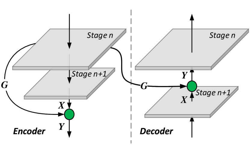
(a) Network Architecture

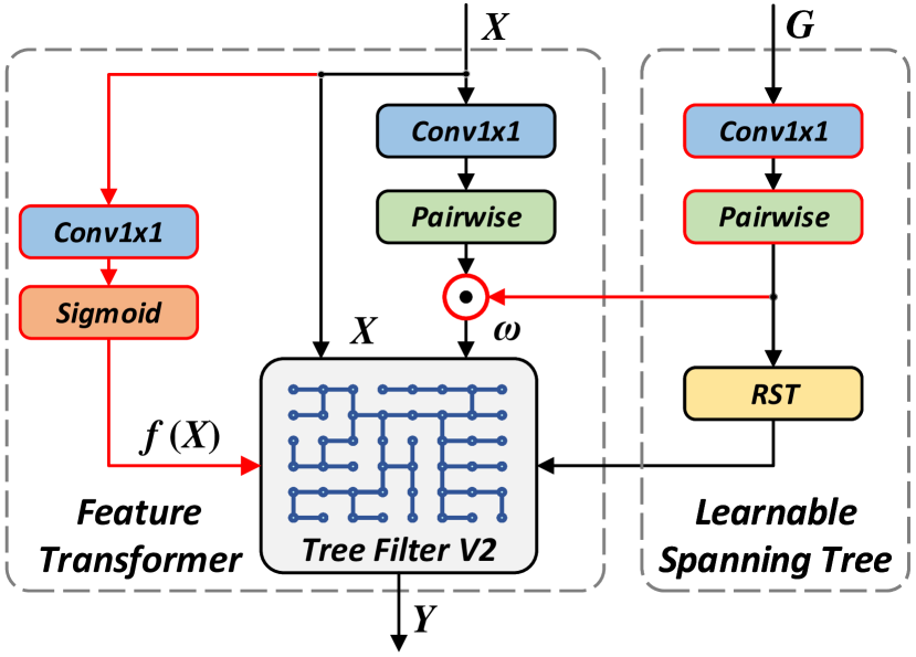
(b) Learnable Tree Filter V2 Module

Figure 2: The diagram of the network architecture and the proposed Learnable Tree Filter V2 module. The green circles in (a) denote the LTF-V2 modules, which generate the spanning tree with the low-level feature (i.e., “Stage n”) and then transform the high-level feature (i.e., “Stage n+1”). We use red in (b) to represent the newly added components compared with the LTF-V1 module. $f({X})$ and $\mathbf{\omega}$ are the elements in unary and pairwise terms, respectively. “RST” denotes the proposed close random spanning tree algorithm. And “Pairwise” indicates calculating the distance for each edge.

Analysis. First of all, we analyze why the LTF-V1 module works well on semantic segmentation. By comparing the formulas, we give a specific MRF on tree $\mathcal{G}_{T}$, which is formally equivalent to the LTF-V1 (the proof is provided in the supplementary material). Specifically, the formulation is shown as Eq. 5 and Eq. 6, where $\delta(\cdot)$ denotes the unit impulse function and ${\rm Desc}_{\mathcal{G}_{T}}(i,j)$ is the descendants of node $j$ when node $i$ is the root of tree $\mathcal{G}_{T}$.

$$\phi_{i}(h_{i},x_{i})\equiv 1,$$ (5)

$$\psi_{i,j}(h_{i},h_{j}):=\left\{\begin{matrix}\delta(h_{i}-h_{j})&h_{i}\notin{\rm Desc}_{\mathcal{G}_{T}}(i,j)\\ {\rm exp}(-\omega_{i,j})\delta(h_{i}-h_{j})&h_{i}\in{\rm Desc}_{\mathcal{G}_{T}}(i,j)\end{matrix}\right.$$ (6)

The MRF is demonstrated to preserve the local structure by modeling data-dependent pairwise terms between adjacent nodes in previous works [21, 36, 37, 38, 39]. This property of MRF is extremely desired by semantic segmentation [40, 41, 42, 43]. Furthermore, combined with the visualizations with rich details [20], we consider the reason for the effectiveness of LTF-V1 on semantic segmentation lies in modeling learnable pairwise terms.

We further analyze why the LTF-V1 module performs unsatisfactorily in the instance-aware tasks. The effective long-range dependencies modeling, which provides powerful semantic representations, is proved to be crucial for instance-aware tasks [17, 15, 18, 16]. However, due to the intrinsic geometric constraint of the LTF-V1, as illustrated in Fig. 1, interactions with distant nodes need to pass through nearby nodes. Meanwhile, as shown in Eq. 5, the LTF-V1 models the unary term as a constant scalar, resulting in the filtering weight monotonously decreases as the distance increase along a path (the proof is provided in the supplementary material). Therefore, these properties force the LTF-V1 to focus on the nearby region, leading to the difficulty of long-range interactions and unsatisfactory performance in instance-aware tasks.

Solution. Eventually, we try to give a solution to address the problem. To focus on the distant region, we need to relax the geometric constraint and allow the filtering weight of distant nodes to be larger than that of close ones. In this paper, motivated by confidence estimation methods [22, 23, 24], we present a learnable unary term which can meet the requirements (the proof is provided in the supplementary material). The formulation is shown on Eq. 7, where $f(\cdot)$ denotes a unary function embedded in the deep neural network and $\beta$ is a learnable parameter. Intuitively, for a node, $f(\cdot)$ reflects the confidence of its input feature, while $\beta$ is the potential for choosing other features.

$$\phi_{i}(h_{i},x_{i}):=\left\{\begin{matrix}f(x_{i})&h_{i}=i\\ {\rm exp}(-\beta)&h_{i}\neq i\end{matrix}\right.$$ (7)

Let Eq. 7 and Eq. 6 substitute into Eq. 4. Since the tree $\mathcal{G}_{T}$ is a acyclic graph, the closed-form solution of Eq. 3 can be derived as Eq. 8 by using the belief propagation algorithm [44]. $z_{i}$ is the normalizing coefficient and $|{E}_{j,i}|$ denotes the number of edges in the path.

$$y_{i}=\frac{1}{z_{i}}\sum_{\forall x_{j}\in{X}}{S_{\mathcal{G}_{T}}({E}_{j,i}){{\rm exp}(-\beta)}^{|{E}_{j,i}|}f(x_{j})x_{j}}.$$ (8)

Accordingly, we define the Eq. 8 as a more generic form of the learnable tree filter, namely the Learnable Tree Filter V2 (LTF-V2). The unary and pairwise terms in the LTF-V2 are complementary and promoting to each other. The unary term on Eq. 7 allows the LTF-V2 to focus on the distant region, bringing more effective long-range interactions. Meanwhile, the data-dependent pairwise term can further refine the distant region to fit detailed structures.

3.4 Learnable Random Spanning Tree

Input: A 4-connected graph $\mathcal{G}$.

Output: Random spanning tree $\mathcal{G}_{T}$.

1 $\mathcal{G}_{T}\leftarrow\emptyset$.

2 for $e\in E(\mathcal{G})$ do

3       $l(e)\leftarrow e.$ $\triangleright$ Initialize a label for each edge.

4while $|V(\mathcal{G})|>1$ do

5       for $v_{i}\in V(\mathcal{G})$ do

6             $e_{i}\sim E_{\mathcal{G}}(v_{i})$. $\triangleright$ Sample an incident edge.

7             $\mathcal{G}_{T}\leftarrow\mathcal{G}_{T}\cup\{l(e_{i})\}$.

8      $\mathrm{Contract}(E(\mathcal{G}))$. $\triangleright$ Contraction algorithm.

9       $\mathrm{Flatten}(\mathcal{G})$. $\triangleright$ Remove loops and parallel edges.

return $\mathcal{G}_{T}$.

Algorithm 1 Close random spanning tree

Although the LTF-V1 module takes the first step to make the tree filtering process [34] trainable, the inside minimum spanning tree algorithm is still not differentiable. This problem prevents it from being entirely learnable. Moreover, the topology of the spanning tree is determined by guided features only. Therefore, the initialization and source selection of guided features could significantly impact the performance in the original design. In this paper, we bridge this gap by proposing a simple architecture and a close random-spanning-tree algorithm, which is briefly introduced in Fig. 2.

Firstly, we propose a simple strategy to make the spanning tree process learnable. As shown in the right dashed rectangle of Fig. 2(b), we calculate the joint affinities by performing the element-wise production on pairwise similarities, which are generated from the input feature ${X}$ and the guided feature ${G}$, respectively. And then, we use the joint affinities as the edge weights $\omega$ for the feature transformer. This strategy creates a gradient tunnel between the guided feature and the output feature ${Y}$ to make the guided feature trainable utilizing the back-propagation algorithm [45].

Moreover, a close random spanning tree algorithm is designed to replace the original minimum spanning tree in the training phase. As illustrated in Alg. 1, the proposed algorithm is a modification of the Boruvka’s algorithm [46], which replaces the minimum selection to the stochastic sampling (line 6 in Alg. 1) according to the edge weights. This algorithm has the ability to regularize the network and avoid falling into local optima, which is resulted from the greedy strategy of the minimum spanning tree. For the reason that the input $\mathcal{G}$ is a 4-connected planar graph, the computational complexity of the proposed algorithm can be reduced to linear on the number of pixels by using the edge contraction operation [47] (line 8 in Alg. 1). In the training phase, the weights of selected edges as well as the sampling distribution will be optimized. Besides, in the inference phase, we still use the minimum spanning tree to keep the results deterministic.

3.5 Network Architecture

Based on the algorithms in Sec. 3.3 and Sec. 3.4, we propose a generic feature transform module, namely the Learnable Tree Filter V2 module (LTF-V2 module). As illustrated in Fig. 2(b), the LTF-V2 module is composed of a feature transformer and a learnable spanning tree process. To highlight the effectiveness of the LTF-V2 module, we adopt a simple embedding operator to instantiate the function $f(\cdot)$ in the unary term, i.e., $f(x_{i})=\mathrm{Sigmoid}(\pi{x_{i}}^{\top})$, where $\pi\in\mathbb{R}^{1\times C}$. In addition, following the design of the LTF-V1 module, we instantiate the pairwise function $S_{\mathcal{G}_{T}}(\cdot)$ of edge weights as the Euclidean distance and adopt the grouping strategy for the edge weights and the unary term. Specifically, the grouping strategy [48] is adopted to split the input feature into specific groups along the channel dimension and aggregate them with different weights. The default group number is set to 16, and the detailed comparison is provided in the supplementary material.

Due to the linear computational complexity, the LTF-V2 module is highly efficient and can be easily embedded as a learnable layer into deep neural networks. To this end, we propose two usages of the module for the encoder and the decoder, respectively. The usage for the encoder is shown as the left part of Fig. 2(a), which embeds the LTF-V2 module between adjacent stages of the encoder. In this way, the resize operation is used on the low-level feature (e.g., the “Stage n" in Fig. 2(a)) when the dimensions of the low-level feature and the high-level feature (e.g., the “Stage n+1" in Fig. 2(a)) are inconsistent. Furthermore, the LTF-V2 module adopts the resized low-level feature as a guided feature ${G}$ to generate the spanning tree and transform the high-level feature. Different from the encoder, the usage for the decoder is shown in the right diagram of Fig. 2(a). The LTF-V2 module is embedded in the decoder and relies on the corresponding low-level feature in the encoder to generate the spanning tree.

In this paper, we conduct experiments on semantic segmentation and instance-aware tasks, i.e., object detection and instance segmentation. For semantic segmentation, the ResNet [26] is adopted as the backbone with the naive decoder following the LTF-V1. While for instance-aware tasks, we adopt the Mask R-CNN [25] with FPN as the decoder and ResNet [26]/ResNeXt [48] as the encoder.

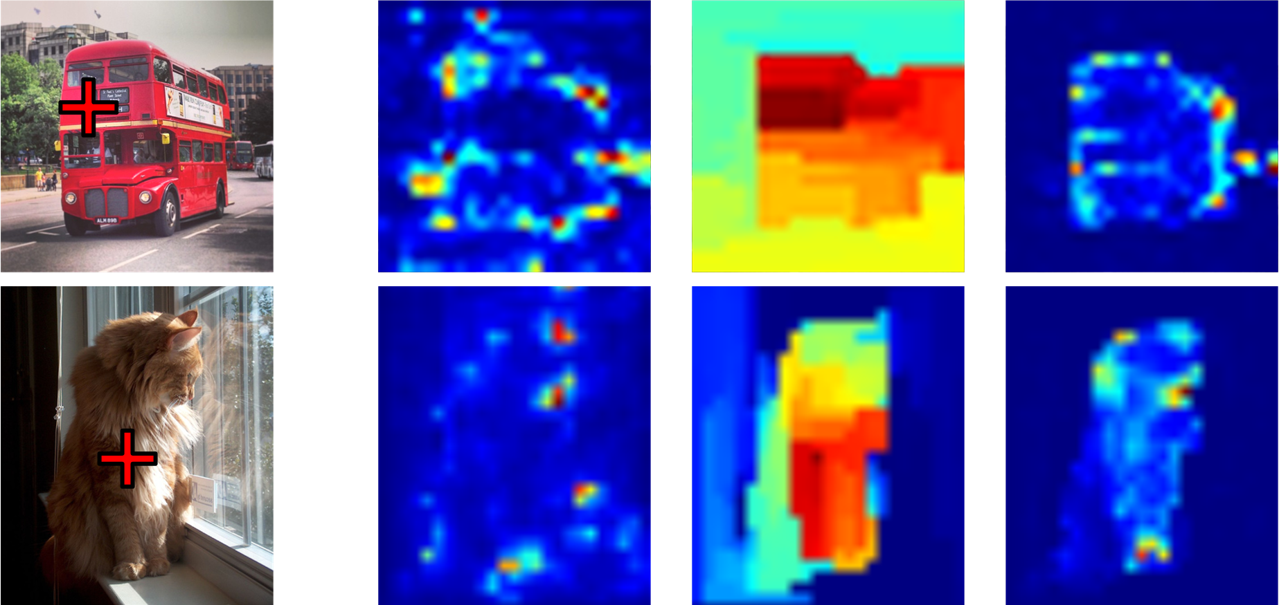
Figure 3: Visualization of the affinity maps in specific positions (marked by the red cross in each image). The affinity maps (from left to right) are generated from the unary term, the pairwise term and the LTF-V2, respectively.

4 Experiments

To demonstrate the effectiveness of the proposed method, several experiments are conducted on COCO [49] for object detection/instance segmentation (instance-aware tasks) and Cityscapes [50] for semantic segmentation.

4.1 Experiments in Instance-aware Tasks

4.1.1 Training Setting

Following the configuration of Mask R-CNN in the Detectron2 [51] framework, we employ the FPN based decoder and a pair of 4-convolution heads for bounding box regression and mask prediction, respectively. All the backbones are pre-trained on the ImageNet classification dataset [52] unless otherwise specified. In the training phase, input images are resized so that the shorter side is 800 pixels. All the hyper-parameters are identical to the 1x schedule in the Detectron2 framework.

4.1.2 Ablation Study

Components of the LTF-V2. Intuitively, as illustrated in Fig. 3, the properties of unary and pairwise terms are complementary. The unary term can guide the LTF-V2 to focus on the coarsely distant regions, and the pairwise term further refines the regions to fit the detailed structures. Furthermore, we give the qualitative comparisons on Tab. 4, which demonstrates the balance of the two terms can work better than the single one. To reveal the impact of the data-dependent spanning tree, we adopt the uniformly random spanning tree [47] for the pairwise term by default.

Table 1: Comparisons among related works and the LTF-V2 module on different stages for COCO 2017 val set. All experiments are conducted on the Mask-RCNN framework with 1x learning rate schedule. GCNet [19] is used after each bottleneck, and other blocks are applied at the end of specific stages in the backbone. The settings of all the models are configured as the original papers.

Model	Stage	$\mathrm{AP}_{box}$	$\mathrm{AP}_{box}^{50}$	$\mathrm{AP}_{box}^{75}$	$\mathrm{AP}_{seg}$	$\mathrm{AP}_{seg}^{50}$	$\mathrm{AP}_{seg}^{75}$	#FLOPs	#Params
ResNet-50 (1x)	-	38.8	58.7	42.4	35.2	55.6	37.6	279.4B	44.4M
+Non-Local [15]	4	39.5	59.6	42.7	35.6	56.7	37.6	+10.67B	+2.09M
+CCNet [16]	345	40.1	60.4	44.1	36.0	57.4	38.4	+16.62B	+6.88M
+LatentGNN [18]	345	40.6	61.3	44.5	36.6	58.1	39.2	+3.59B	+1.07M
+GCNet [19]	All	40.7	61.0	44.2	36.7	58.1	39.2	+0.35B	+10.0M
+LTF-V1	345	40.0	60.4	43.7	36.1	57.5	38.4	+0.31B	+0.06M
+LTF-V2	3	40.1	59.9	43.9	36.0	57.1	38.3	+0.43B	+0.02M
	4	40.6	61.0	44.4	36.6	58.2	39.0	+0.26B	+0.04M
	5	40.2	60.5	43.6	36.1	57.5	38.4	+0.17B	+0.08M
	345	41.2	61.6	45.2	37.0	58.4	39.5	+0.68B	+0.14M

Table 2: Comparison of different spanning tree algorithms for the LTF-V2 module on COCO 2017 val set. MST and LST are the minimum spanning tree algorithm and the proposed learnable spanning tree algorithm, respectively. Pretrain indicates the pre-trained weights for the backbone.

Pretrain	MST	LST	$\mathrm{AP}_{box}$	$\mathrm{AP}_{seg}$
Scratch	✓	✗	29.4	26.7
	✗	✓	30.3	27.6
ImageNet [52]	✓	✗	40.9	36.8
	✗	✓	41.2	37.0

Table 3: Comparisons among different backbones for the Mask-RCNN framework on COCO 2017 val set.

Model	$\mathrm{AP}_{box}$	$\mathrm{AP}_{seg}$
ResNet-101 (1x)	40.7	36.6
+LTF-V1	41.6	37.3
+LTF-V2	42.5	38.0
ResNeXt-101 (1x)	43.0	38.3
+LTF-V1	43.8	39.0
+LTF-V2	44.5	39.7
ResNeXt-101 + Cascade (1x)	45.5	39.3
+LTF-V1	46.2	40.0
+LTF-V2	46.9	40.4

Stages. We explore the effect when inserting the LTF-V2 module after the last layer of different stages. The performance in stage 4 is better than in stage 3 and stage 5, which reflects the advantage of using both semantic context and detailed structure. Moreover, due to the efficiency of our proposed framework, we can further insert the LTF-V2 module into multiple stages to fuse multi-scale features. In this way, as shown in Tab. 1, our method achieves 41.2% on $\rm{AP}^{box}$ and 37.0% on $\rm{AP}^{seg}$, which has 2.4% and 1.8% absolute gains over the baseline on $\rm{AP}^{box}$ and $\rm{AP}^{seg}$, respectively.

Spanning tree algorithm. To evaluate the proposed learnable spanning tree algorithm, we conduct ablation studies with the original minimum spanning tree algorithm. As shown in Tab. 3, the results demonstrate the effectiveness of the proposed learnable spanning tree algorithm, which achieves consistent improvements on both localization and segmentation. Especially without pre-training, the improvement is more prominent, which indicates that the proposed algorithm improves the robustness to alleviate the adverse impact of random initialization.

Stronger backbones. To further validate the effectiveness, we evaluate the proposed LTF-V2 modules on stronger backbones. As shown in Tab. 3, we adopt ResNet-101 or ResNeXt-101 as the backbone. Following the same strategy, we insert the learnable tree filter modules at the end of stage3, stage4, and stage5, respectively. The LTF-V2 module still achieves noticeable performance gains over stronger baselines. Specifically, when using cascade strategy [53] and ResNeXt-101 as the backbone, we achieve 1.4% and 1.1% absolute gains over the baseline for $\rm{AP}^{box}$ and $\rm{AP}^{seg}$, respectively.

4.2 Experiments on Semantic Segmentation

4.2.1 Training Setting

For semantic segmentation, training images are randomly resized by 0.5 to 2.0$\times$ and cropped to 1024$\times$1024. The random flipping horizontally is applied for data augmentation. Furthermore, we employ 8 GPUs for training, and the effective mini-batch size is 16. Following conventional protocols [31, 43, 20], we set the initial learning rate to 0.01 and employ the “poly" schedule (i.e., multiply $(1-\frac{iter}{max\_iter})^{power}$ for each iteration) with $\mathrm{power}=0.9$. All models are optimized by using synchronized SGD with the weight decay of 0.0001 and the momentum of 0.9. For fair comparisons, we adopt the LTF-V2 modules in each stage of the decoder as the LTF-V1 does.

4.2.2 Ablation Study

As shown in Tab. 6, we give quantitative comparisons between the LTF-V1 module and the LTF-V2 module. The results show that both yield significant improvement over the baseline. Specifically, without data augmentation, the LTF-V2 module achieves 4.5% and 1.5% absolute gains on mIoU over the baseline and the LTF-V1 module, respectively. Moreover, we adopt multi-scale and flipping augmentations for testing. The performance of the LTF-V2 module is further improved, which still attains 3.4% and 1.7% absolute gains on mIoU over the baseline and the LTF-V1 module, respectively.

Table 4: Comparisons among different components of the LTF-V2 module on COCO 2017 val set. Unary and Pairwise are the components of the proposed MRF, where the pairwise term adopts the uniformly random spanning tree by default. LST is the proposed learnable spanning tree algorithm.

Model	Unary	Pairwise	LST	$\mathrm{AP}_{box}$	$\mathrm{AP}_{box}^{50}$	$\mathrm{AP}_{box}^{75}$	$\mathrm{AP}_{seg}$	$\mathrm{AP}_{seg}^{50}$	$\mathrm{AP}_{seg}^{75}$
ResNet-50 (1x)	✗	✗	✗	38.8	58.7	42.4	35.2	55.6	37.6
	✓	✗	✗	39.7	59.7	43.5	35.8	56.8	38.1
	✗	✓	✗	39.6	59.5	43.3	35.7	56.6	37.9
	✓	✓	✗	40.7	61.2	44.8	36.7	58.2	39.3
	✗	✓	✓	40.2	60.7	43.8	36.2	57.4	38.8
	✓	✓	✓	41.2	61.6	45.2	37.0	58.4	39.5

Table 5: The ablation studies conducted on Cityscapes val set. MS and Flip denote adopting multi-scale and flipping augmentation for testing, respectively.

Model	MS&Flip	mIoU (%)	mAcc (%)
ResNet-50	✗	72.9	95.5
+LTF-V1	✗	75.9	95.8
+LTF-V2	✗	77.4	96.0
ResNet-50	✓	75.5	95.9
+LTF-V1	✓	77.2	96.0
+LTF-V2	✓	78.9	96.1

Table 6: Comparisons with state-of-the-art results on Cityscapes test set. Our model is trained with fine annotations only.

Model	Backbone	mIoU (%)
PSPNet [13]	ResNet-101	78.4
DFN [43]	ResNet-101	79.3
DenseASPP [54]	DenseNet-161	80.6
LTF-V1 [20]	ResNet-101	80.8
CCNet [16]	ResNet-101	81.4
DANet [55]	ResNet-101	81.5
SPNet [56]	ResNet-101	82.0
Ours (LTF-V2)	ResNet-101	82.1

4.2.3 Comparison with State-of-the-arts

To further improve the performance, we adopt a global average pooling operation and an additional ResBlocks [26] in the decoder, which follows the design in the LTF-V1 module. Specifically, an extra global average pooling operator is inserted at the end of stage4 in the encoder. In addition, multiple ResBlocks based on “Conv3$\times$3" are added before each upsampling operator in the decoder. Similar with the conventional protocols [31, 43, 20], we further finetune our model on both train and val sets. As shown in Tab. 6, we achieve 82.1% mIoU result on Cityscapes test set, which is superior to other state-of-the-art approaches with ResNet-101 backbone and only fine annotations.

5 Conclusion

In this paper, we first rethink the advantages and shortages of the LTF-V1 by reformulating it as a Markov Random Field. Then we present a learnable unary term to relax the geometric constraint and enable effectively long-range interactions. Besides, we propose the learnable spanning tree algorithm to replace the non-differentiable one for an entirely learnable tree filter. Extensive ablation studies are conducted to elaborate on the effectiveness and efficiency of the proposed method, which is demonstrated to bring significant improvements on both instance-aware tasks and semantic segmentation with negligible computational overhead. We hope that the perspective of Markov Random Field for context modeling can provide insights into future works, and beyond.

Broader Impact

Context modeling is a powerful tool to improve the ability for feature representation, which has been widely applied in real-world scenarios, e.g., computer vision and natural language processing. The traditional tree filter [34] already has great impacts on many low-level computer vision tasks, owing to its structure-preserving property and high efficiency. This paper further releases its representation potential by relaxing the geometric constraint. Specifically, our method provides a new perspective for context modeling by unifying the learnable tree filter with the Markov Random Field, which is further demonstrated to be effective in several vision tasks with negligible computational and parametric overheads. These properties of our method have great potentials, which allow our method and principle to extend to other complex tasks with large-number nodes, e.g., replacing the attention module of transformer for natural language processing and enhancing sequential representation for video analysis.

Appendix A Visualization

In this section, as shown in Fig. 4 and Fig. 5, we present several visualization results of the baseline (w/o context block) and the proposed LTF-V2 module for instance-aware tasks and semantic segmentation, respectively.

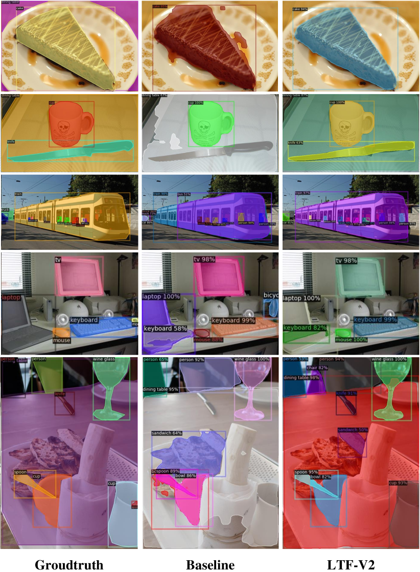
Figure 4: Visualization results on COCO 2017 val set. We use different colors to distinguish between instances that do not represent categories. The results demonstrate the superiority of the LTF-V2 module in terms of both semantics and details

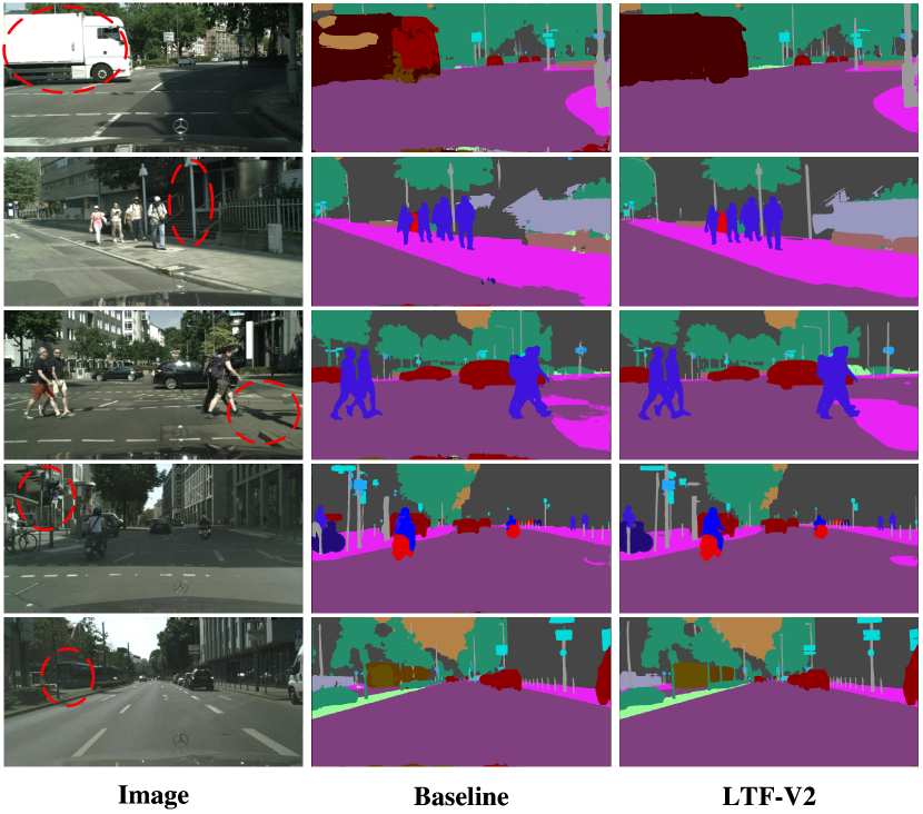
Figure 5: Visualization results on Cityscapes val set. The red dotted ellipses indicate the area of the major difference between the baseline and the LTF-V2 module

Appendix B Algorithm Proof

In this section, we present the detailed proofs for the claims about the learnable tree filter. Please note that the symbols follow the definitions in the main paper.

Lemma 1.

Given a Markov Random Field on the tree $\mathcal{G}_{T}$, whose unary and pairwise terms are the Eq. 9 and the Eq. 10 respectively, the marginal probability of latent variable satisfies $P_{\mathcal{G}_{T}}(h_{i}=j)=\frac{1}{z_{i}}S_{\mathcal{G}_{T}}(\mathbf{E}_{j,i})$.

$$\phi_{i}(h_{i},x_{i})\equiv 1,$$ (9)

$$\psi_{i,j}(h_{i},h_{j}):=\left\{\begin{matrix}\delta(h_{i}-h_{j})&h_{i}\notin{\rm{Desc}}_{\mathcal{G}_{T}}(i,j)\\ {\rm{exp}}(-\omega_{i,j})\delta(h_{i}-h_{j})&h_{i}\in{\rm{Desc}}_{\mathcal{G}_{T}}(i,j)\end{matrix}\right.$$ (10)

Proof.

To obtain the marginal probability of the Markov Random Field on an acyclic graph, we adopt the belief propagation algorithm as shown on Eq. 11, where $\mathcal{N}_{i}$ denotes the set of adjacent nodes of node $i$ in the tree.

$$P_{\mathcal{G}_{T}}(h_{i}) =\frac{1}{z_{i}}\phi_{i}(h_{i},x_{i})\prod_{\forall j\in\mathcal{N}_{i}}m_{j,i}(h_{i}),$$ (11)

$$m_{j,i}(h_{i}) =\sum_{\forall h_{j}\in\mathcal{V}}{\phi_{j}(h_{j},x_{j})\psi_{j,i}(h_{j},h_{i})\prod_{\forall k\in\mathcal{N}_{j}\setminus i}m_{k,j}(h_{j}).}$$

For $h_{i}=i$, the marginal probability is

$$P_{\mathcal{G}_{T}}(h_{i}=i)=\frac{1}{z_{i}}\prod_{\forall j\in\mathcal{N}_{i}}m_{j,i}(i)$$ (12)

$$=\frac{1}{z_{i}}\prod_{\forall j\in\mathcal{N}_{i}}({\sum_{\forall h_{j}\in\mathcal{V}}{\delta(h_{j}-i)\prod_{\forall k\in\mathcal{N}_{j}\setminus i}m_{k,j}(h_{j})}})$$

$$=\frac{1}{z_{i}}\prod_{\forall j\in\mathcal{N}_{i}}{\prod_{\forall k\in\mathcal{N}_{j}\setminus i}m_{k,j}(i)}$$

$$=\frac{1}{z_{i}}\prod_{\forall j\in\mathcal{N}_{i}}{\prod_{\forall k\in\mathcal{N}_{j}\setminus i}\prod_{\forall u\in\mathcal{N}_{k}\setminus k}\cdots 1}$$

$$=\frac{1}{z_{i}}.$$

For $h_{i}=u$ and $u\neq i$, the marginal probability is

$$P_{\mathcal{G}_{T}}(h_{i}=u)=\frac{1}{z_{i}}\prod_{\forall j\in\mathcal{N}_{i}\cap\{p\mid x_{u}\in{\rm Desc}(i,p)\}}m_{j,i}(u)$$ (13)

$$=\frac{1}{z_{i}}{\sum_{\forall h_{j}\in\mathcal{V}}{\psi_{j,i}(h_{j},u)\prod_{\forall k\in\mathcal{N}_{j}\setminus i}m_{k,j}(h_{j})}}$$

$$=\frac{1}{z_{i}}{\sum_{\forall h_{j}\in\mathcal{V}}{\rm exp}(-\omega_{j,i}){\delta(h_{j}-u)\prod_{\forall k\in\mathcal{N}_{j}\setminus i}m_{k,j}(h_{j})}}$$

$$=\frac{1}{z_{i}}{\rm exp}(-\omega_{j,i})\prod_{\forall k\in\mathcal{N}_{j}\setminus i}m_{k,j}(u)$$

$$=\frac{1}{z_{i}}{\rm exp}(-\omega_{j,i}){\rm exp}(-\omega_{k,j})\cdots\prod_{\forall v\in\mathcal{N}_{u}\setminus par(u)}m_{v,u}(u)$$

$$=\frac{1}{z_{i}}{\rm exp}(-\omega_{j,i}){\rm exp}(-\omega_{k,j})\cdots{\rm exp}(-\omega_{u,par(u)})$$

$$=\frac{1}{z_{i}}\prod_{\forall(k,m)\in\mathbf{E}_{j,i}}{{\rm exp}(-\omega_{k,m})}.$$

Therefore, $P_{\mathcal{G}_{T}}(h_{i}=j)=\frac{1}{z_{i}}S_{\mathcal{G}_{T}}(\mathbf{E}_{j,i})$.

∎

Lemma 2.

Given a Markov Random Field on the tree $\mathcal{G}_{T}$, whose unary and pairwise terms are the Eq. 9 and the Eq. 10, respectively. When denoting node $i$ as the root of the tree $\mathcal{G}_{T}$ and node $v$ (distant) as one of the descendants node of node $u$ (nearby), the marginal probability of latent variable satisfies $P_{\mathcal{G}_{T}}(h_{i}=v)\leq P_{\mathcal{G}_{T}}(h_{i}=u)$.

Proof.

Since the edge distance satisfies $\omega_{k,m}\geq 0$, the marginal probability of latent variable satisfies

$$P_{\mathcal{G}_{T}}(h_{i}=v)=\frac{1}{z_{i}}S_{\mathcal{G}_{T}}(\mathbf{E}_{v,i})$$ (14)

$$=\frac{1}{z_{i}}S_{\mathcal{G}_{T}}(\mathbf{E}_{u,i})S_{\mathcal{G}_{T}}(\mathbf{E}_{v,u})$$

$$=P_{\mathcal{G}_{T}}(h_{i}=u)\prod_{\forall(k,m)\in\mathbf{E}_{v,u}}{{\rm exp}(-\omega_{k,m})}$$

$$\leq P_{\mathcal{G}_{T}}(h_{i}=u).$$

∎

Lemma 3.

Given a Markov Random Field on the tree $\mathcal{G}_{T}$, whose unary and pairwise terms are the Eq. 15 and the Eq. 10, respectively. When denoting node $i$ as the root of the tree $\mathcal{G}_{T}$ and node $v$ (distant) as one of the descendants of node $u$ (nearby), there exists a specific pair of $f(\cdot)$ and $\beta$, such that the marginal probability of latent variable satisfies $P_{\mathcal{G}_{T}}(h_{i}=v)>P_{\mathcal{G}_{T}}(h_{i}=u)$.

$$\phi_{i}(h_{i},x_{i}):=\left\{\begin{matrix}f(x_{i})&h_{i}=i\\ {\rm{exp}}(-\beta)&h_{i}\neq i\end{matrix}\right.$$ (15)

Proof.

For $h_{i}=v$, the marginal probability is

$$P_{\mathcal{G}_{T}}(h_{i}=v)=\frac{1}{z_{i}}{{\rm{exp}}(-\beta)}^{|\mathbf{E}_{v,i}|}f(x_{v})S_{\mathcal{G}_{T}}(\mathbf{E}_{v,i})$$ (16)

$$=\frac{1}{z_{i}}{{\rm{exp}}(-\beta)}^{|\mathbf{E}_{u,i}|}S_{\mathcal{G}_{T}}(\mathbf{E}_{u,i})f(x_{v}){{\rm{exp}}(-\beta)}^{|\mathbf{E}_{v,u}|}S_{\mathcal{G}_{T}}(\mathbf{E}_{v,u})$$

$$=P_{\mathcal{G}_{T}}(h_{i}=u)\frac{f(x_{v})}{f(x_{u})}\prod_{\forall(k,m)\in\mathbf{E}_{v,u}}{{\rm exp}(-\omega_{k,m}-\beta)}.$$

When $\frac{f(x_{v})}{f(x_{u})}\prod_{\forall(k,m)\in\mathbf{E}_{v,u}}{{\rm exp}(-\omega_{k,m}-\beta)}>1$, the marginal probability of latent variable satisfies $P_{\mathcal{G}_{T}}(h_{i}=v)>P_{\mathcal{G}_{T}}(h_{i}=u)$. ∎

Appendix C Runtime

Due to trees are acyclic graphs, we can adopt a well-designed dynamic programming algorithm to reduce the computational complexity to linear w.r.t vertex number. Besides, in order to improve the efficiency on GPU devices, we parallelize the algorithm along with batches, channels, and nodes of the same depth. As shown in Fig. 6, the empirical runtime of our method is far less than that of the Non-Local network [12], which uses an extremely sophisticated tensor library. We believe that the efficiency of LTF-V2 can be further improved through device-oriented code optimization.

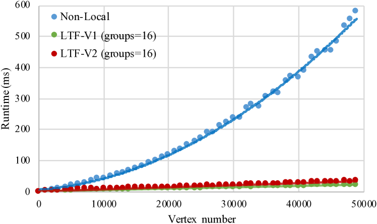
Figure 6: Comparisons of the runtime on a Tesla V100 GPU among LTF-V1, LTF-V2 and Non-Local network. The number of feature channels is set to 512

Appendix D Additional Ablation Study

Table 7: Comparisons among different positions and different groups on COCO 2017 val set when using ResNet-50 as our backbone. Enc and Dec denote embedding the blocks in the backbone and the FPN, respectively

Model	Position	Groups	$\mathrm{AP}_{box}$	$\mathrm{AP}_{box}^{50}$	$\mathrm{AP}_{box}^{75}$	$\mathrm{AP}_{seg}$	$\mathrm{AP}_{seg}^{50}$	$\mathrm{AP}_{seg}^{75}$	#FLOPs	#Params
+LTF-V1	Dec	16	39.6	60.0	43.4	35.8	56.9	38.0	+0.45B	+0.02M
	Enc	1	39.6	59.6	43.1	35.6	56.5	37.9	+0.09B	+0.01M
	Enc	16	40.0	60.4	43.7	36.1	57.5	38.4	+0.31B	+0.06M
+LTF-V2	Dec	16	39.9	60.1	43.6	36.0	57.1	38.4	+1.23B	+0.06M
	Enc	1	40.2	60.5	44.0	36.3	57.5	38.8	+0.13B	+0.01M
	Enc	4	40.9	61.3	44.5	36.8	58.4	39.4	+0.24B	+0.04M
	Enc	8	40.9	61.4	44.3	36.8	58.4	39.2	+0.39B	+0.07M
	Enc	16	41.2	61.6	45.2	37.0	58.4	39.5	+0.68B	+0.14M
	Enc	32	41.1	61.6	44.8	37.0	58.7	39.4	+1.28B	+0.29M

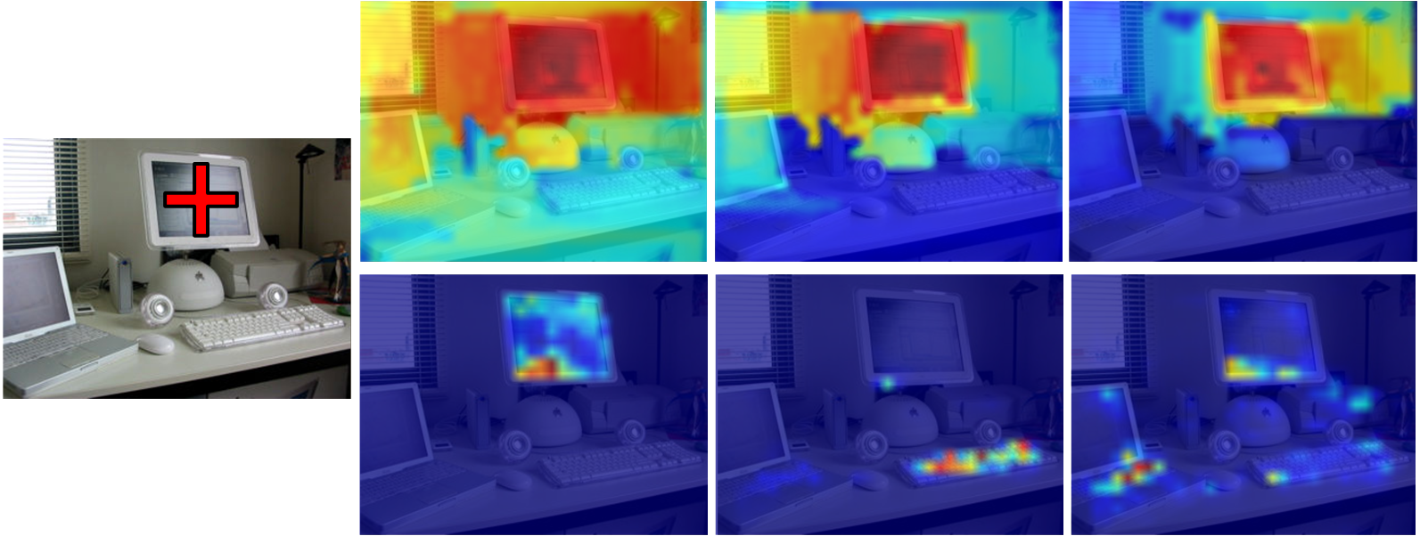
(a) Affinity maps of LTF-V1 (top) and LTF-V2 (bottom) with different groups

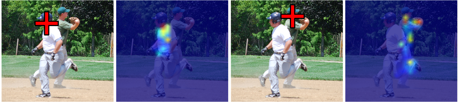
(b) Affinity maps of LTF-V2 for different instances

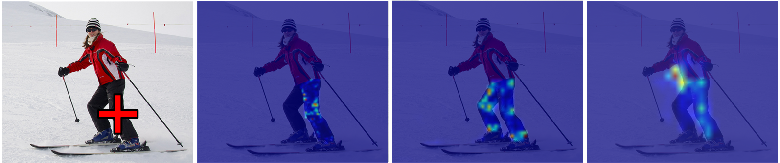
(c) Affinity maps of LTF-V2 in different stages

Figure 7: Visualization of the affinity maps in specific positions (marked by the red cross in each image). The responses of different groups, instances, and stages are illustrated in (a), (b), and (c), respectively. The figure (a) intuitively shows that the diversity of the LTF-V2 module is significantly higher than that of the LTF-V1 module due to the relaxation of geometric constraints. The figure (b) reveals that the LTF-V2 module is aware of the structure of instance, even when the instances of the same category are overlapping. Besides, the heat maps (from left to right) in (c) correspond to stage3, stage4, and stage5 in the encoder, respectively.

References

- [1] Liang-Chieh Chen, George Papandreou, Iasonas Kokkinos, Kevin Murphy, and Alan L Yuille. Semantic image segmentation with deep convolutional nets and fully connected crfs. In International Conference on Learning Representations, 2015.
- [2] Loic Landrieu and Martin Simonovsky. Large-scale point cloud semantic segmentation with superpoint graphs. In IEEE Conference on Computer Vision and Pattern Recognition, 2018.
- [3] Karen Simonyan and Andrew Zisserman. Very deep convolutional networks for large-scale image recognition. In International Conference on Learning Representations, 2014.
- [4] Christian Szegedy, Wei Liu, Yangqing Jia, Pierre Sermanet, Scott Reed, Dragomir Anguelov, Dumitru Erhan, Vincent Vanhoucke, and Andrew Rabinovich. Going deeper with convolutions. In IEEE Conference on Computer Vision and Pattern Recognition, 2015.
- [5] Lin Song, Shiwei Zhang, Gang Yu, and Hongbin Sun. Tacnet: Transition-aware context network for spatio-temporal action detection. In IEEE Conference on Computer Vision and Pattern Recognition, 2019.
- [6] Yanwei Li, Lin Song, Yukang Chen, Zeming Li, Xiangyu Zhang, Xingang Wang, and Jian Sun. Learning dynamic routing for semantic segmentation. In IEEE Conference on Computer Vision and Pattern Recognition, 2020.
- [7] Shiwei Zhang, Lin Song, Changxin Gao, and Nong Sang. Glnet: Global local network for weakly supervised action localization. IEEE Transactions on Multimedia, 2019.
- [8] Lin Song, Yanwei Li, Zhengkai Jiang, Zeming Li, Hongbin Sun, Jian Sun, and Nanning Zheng. Fine-grained dynamic head for object detection. Advances in Neural Information Processing Systems, 2020.
- [9] Wenjie Luo, Yujia Li, Raquel Urtasun, and Richard Zemel. Understanding the effective receptive field in deep convolutional neural networks. In Advances in Neural Information Processing Systems, 2016.
- [10] Liang-Chieh Chen, George Papandreou, Florian Schroff, and Hartwig Adam. Rethinking atrous convolution for semantic image segmentation. arXiv preprint arXiv:1706.05587, 2017.
- [11] Liang-Chieh Chen, Yukun Zhu, George Papandreou, Florian Schroff, and Hartwig Adam. Encoder-decoder with atrous separable convolution for semantic image segmentation. In European Conference on Computer Vision, 2018.
- [12] Jifeng Dai, Haozhi Qi, Yuwen Xiong, Yi Li, Guodong Zhang, Han Hu, and Yichen Wei. Deformable convolutional networks. In IEEE International Conference on Computer Vision, 2017.
- [13] Hengshuang Zhao, Jianping Shi, Xiaojuan Qi, Xiaogang Wang, and Jiaya Jia. Pyramid scene parsing network. In IEEE Conference on Computer Vision and Pattern Recognition, 2017.
- [14] Liang-Chieh Chen, George Papandreou, Iasonas Kokkinos, Kevin Murphy, and Alan L Yuille. Deeplab: Semantic image segmentation with deep convolutional nets, atrous convolution, and fully connected crfs. IEEE Transactions on Pattern Analysis and Machine Intelligence, 2017.
- [15] Xiaolong Wang, Ross Girshick, Abhinav Gupta, and Kaiming He. Non-local neural networks. In IEEE Conference on Computer Vision and Pattern Recognition, 2018.
- [16] Zilong Huang, Xinggang Wang, Lichao Huang, Chang Huang, Yunchao Wei, and Wenyu Liu. Ccnet: Criss-cross attention for semantic segmentation. In IEEE International Conference on Computer Vision, 2019.
- [17] Han Hu, Jiayuan Gu, Zheng Zhang, Jifeng Dai, and Yichen Wei. Relation networks for object detection. In IEEE Conference on Computer Vision and Pattern Recognition, 2018.
- [18] Songyang Zhang, Shipeng Yan, and Xuming He. Latentgnn: Learning efficient non-local relations for visual recognition. In International Conference on Machine Learning, 2019.
- [19] Yue Cao, Jiarui Xu, Stephen Lin, Fangyun Wei, and Han Hu. Gcnet: Non-local networks meet squeeze-excitation networks and beyond. arXiv preprint arXiv:1904.11492, 2019.
- [20] Lin Song, Yanwei Li, Zeming Li, Gang Yu, Hongbin Sun, Jian Sun, and Nanning Zheng. Learnable tree filter for structure-preserving feature transform. In Advances in Neural Information Processing Systems, 2019.
- [21] Stan Z Li. Markov random field models in computer vision. In European Conference on Computer Vision, 1994.
- [22] Matteo Poggi, Fabio Tosi, and Stefano Mattoccia. Quantitative evaluation of confidence measures in a machine learning world. In IEEE International Conference on Computer Vision, 2017.
- [23] Fabio Tosi, Matteo Poggi, Antonio Benincasa, and Stefano Mattoccia. Beyond local reasoning for stereo confidence estimation with deep learning. In European Conference on Computer Vision, 2018.
- [24] Min-Gyu Park and Kuk-Jin Yoon. Leveraging stereo matching with learning-based confidence measures. In IEEE Conference on Computer Vision and Pattern Recognition, 2015.
- [25] Kaiming He, Georgia Gkioxari, Piotr Dollár, and Ross Girshick. Mask r-cnn. In IEEE International Conference on Computer Vision, 2017.
- [26] Kaiming He, Xiangyu Zhang, Shaoqing Ren, and Jian Sun. Deep residual learning for image recognition. In IEEE Conference on Computer Vision and Pattern Recognition, 2016.
- [27] Kaiming He, Xiangyu Zhang, Shaoqing Ren, and Jian Sun. Spatial pyramid pooling in deep convolutional networks for visual recognition. IEEE Transactions on Pattern Analysis and Machine Intelligence, 2015.
- [28] Fisher Yu and Vladlen Koltun. Multi-scale context aggregation by dilated convolutions. In International Conference on Learning Representations, 2015.
- [29] Ashish Vaswani, Noam Shazeer, Niki Parmar, Jakob Uszkoreit, Llion Jones, Aidan N Gomez, Łukasz Kaiser, and Illia Polosukhin. Attention is all you need. In Advances in Neural Information Processing Systems, 2017.
- [30] Peter Battaglia, Razvan Pascanu, Matthew Lai, Danilo Jimenez Rezende, et al. Interaction networks for learning about objects, relations and physics. In Advances in Neural Information Processing Systems, 2016.
- [31] Changqian Yu, Jingbo Wang, Chao Peng, Changxin Gao, Gang Yu, and Nong Sang. Bisenet: Bilateral segmentation network for real-time semantic segmentation. In European Conference on Computer Vision, 2018.
- [32] Hengshuang Zhao, Yi Zhang, Shu Liu, Jianping Shi, Chen Change Loy, Dahua Lin, and Jiaya Jia. Psanet: Point-wise spatial attention network for scene parsing. In European Conference on Computer Vision, 2018.
- [33] Jie Hu, Li Shen, Samuel Albanie, Gang Sun, and Andrea Vedaldi. Gather-excite: Exploiting feature context in convolutional neural networks. In Advances in Neural Information Processing Systems, 2018.
- [34] Qingxiong Yang. Stereo matching using tree filtering. IEEE Transactions on Pattern Analysis and Machine Intelligence, 2015.
- [35] Joseph B Kruskal. On the shortest spanning subtree of a graph and the traveling salesman problem. Proceedings of the American Mathematical Society, 1956.
- [36] Jianbo Shi and Jitendra Malik. Normalized cuts and image segmentation. IEEE Transactions on Pattern Analysis and Machine Intelligence, 2000.
- [37] Yuri Boykov, Olga Veksler, and Ramin Zabih. Fast approximate energy minimization via graph cuts. IEEE Transactions on Pattern Analysis and Machine Intelligence, 2001.
- [38] Jian Sun, Nan-Ning Zheng, and Heung-Yeung Shum. Stereo matching using belief propagation. IEEE Transactions on Pattern Analysis and Machine Intelligence, 2003.
- [39] Pedro F Felzenszwalb and Daniel P Huttenlocher. Efficient belief propagation for early vision. International Journal of Computer Vision, 2006.
- [40] Liang-Chieh Chen, George Papandreou, Iasonas Kokkinos, Kevin Murphy, and Alan L Yuille. Deeplab: Semantic image segmentation with deep convolutional nets, atrous convolution, and fully connected crfs. IEEE Transactions on Pattern Analysis and Machine Intelligence, 2018.
- [41] Ziwei Liu, Xiaoxiao Li, Ping Luo, Chen Change Loy, and Xiaoou Tang. Deep learning markov random field for semantic segmentation. IEEE Transactions on Pattern Analysis and Machine Intelligence, 2017.
- [42] Shuai Zheng, Sadeep Jayasumana, Bernardino Romera-Paredes, Vibhav Vineet, Zhizhong Su, Dalong Du, Chang Huang, and Philip HS Torr. Conditional random fields as recurrent neural networks. In IEEE International Conference on Computer Vision, 2015.
- [43] Changqian Yu, Jingbo Wang, Chao Peng, Changxin Gao, Gang Yu, and Nong Sang. Learning a discriminative feature network for semantic segmentation. In IEEE Conference on Computer Vision and Pattern Recognition, 2018.
- [44] Jonathan S Yedidia, William T Freeman, and Yair Weiss. Generalized belief propagation. In Advances in Neural Information Processing Systems, 2001.
- [45] Yann LeCun, Yoshua Bengio, and Geoffrey Hinton. Deep learning. Nature, 2015.
- [46] David Eppstein. Spanning trees and spanners. Handbook of Computational Geometry, 1999.
- [47] Jonathan L Gross and Jay Yellen. Graph theory and its applications. CRC press, 2005.
- [48] Saining Xie, Ross Girshick, Piotr Dollár, Zhuowen Tu, and Kaiming He. Aggregated residual transformations for deep neural networks. In IEEE Conference on Computer Vision and Pattern Recognition, 2017.
- [49] Tsung-Yi Lin, Michael Maire, Serge Belongie, James Hays, Pietro Perona, Deva Ramanan, Piotr Dollár, and C Lawrence Zitnick. Microsoft coco: Common objects in context. In European Conference on Computer Vision, 2014.
- [50] Marius Cordts, Mohamed Omran, Sebastian Ramos, Timo Rehfeld, Markus Enzweiler, Rodrigo Benenson, Uwe Franke, Stefan Roth, and Bernt Schiele. The cityscapes dataset for semantic urban scene understanding. In IEEE Conference on Computer Vision and Pattern Recognition, 2016.
- [51] Yuxin Wu, Alexander Kirillov, Francisco Massa, Wan-Yen Lo, and Ross Girshick. Detectron2. https://github.com/facebookresearch/detectron2, 2019.
- [52] Jia Deng, Wei Dong, Richard Socher, Li-Jia Li, Kai Li, and Li Fei-Fei. Imagenet: A large-scale hierarchical image database. In IEEE Conference on Computer Vision and Pattern Recognition, 2009.
- [53] Zhaowei Cai and Nuno Vasconcelos. Cascade r-cnn: Delving into high quality object detection. In IEEE Conference on Computer Vision and Pattern Recognition, 2018.
- [54] Maoke Yang, Kun Yu, Chi Zhang, Zhiwei Li, and Kuiyuan Yang. Denseaspp for semantic segmentation in street scenes. In IEEE Conference on Computer Vision and Pattern Recognition, 2018.
- [55] Jun Fu, Jing Liu, Haijie Tian, Yong Li, Yongjun Bao, Zhiwei Fang, and Hanqing Lu. Dual attention network for scene segmentation. In IEEE Conference on Computer Vision and Pattern Recognition, 2019.
- [56] Qibin Hou, Li Zhang, Ming-Ming Cheng, and Jiashi Feng. Strip pooling: Rethinking spatial pooling for scene parsing. In IEEE Conference on Computer Vision and Pattern Recognition, 2020.