Extending Friedmann equations using fractional derivatives using a Last Step Modification technique: the case of a matter dominated accelerated expanding Universe.

Abstract

We present a toy model for extending the Friedmann equations of relativistic cosmology using fractional derivatives. We do this by replacing the integer derivatives, in a few well-known cosmological results with fractional derivatives leaving their order as a free parameter. All this with the intention to explain the current observed acceleration of the Universe. We apply the Last Step Modification technique of fractional calculus to construct some useful fractional equations of cosmology. The fits of the unknown fractional derivative order and the fractional cosmographic parameters to SN Ia data shows that this simple construction can explain the current accelerated expansion of the Universe without the use of a dark energy component with a MOND-like behaviour using Milgrom’s acceleration constant which sheds light into to the non-necessity of a dark matter component as well.

I Introduction

The Hilbert–Einstein field equations, a success of general relativity, work tremendously well at mass-to-length scales similar to those of the solar system [see e.g. 1], where the gravitational field is moderately weak [2, 3, 4, 5, 6, 7, 8, 9, 10, 11, 12, 13, 14]. At very large mass-to-length ratios, where the gravitational field is very strong, the detection of gravitational waves produced by the interactions of compact objects such as black holes and neutron stars has shown a remarkable good agreement with the predictions of general relativity.

When the Newtonian acceleration of a test particle reaches values $a_{0}\lesssim 10^{-10}\textrm{m}/\textrm{s}^{2}$, or equivalently when the mass-to-length ratios are much smaller than those of the solar system [15], the Hilbert–Einstein field equations cannot fit an enormous amount of astrophysical and cosmological data unless: (a) extra dark matter and/or dark energy components are added or (b) the curvature caused by the matter and energy requires extensions or modifications. In other words, the Hilbert–Einstein field equations do not correctly predict the observed results at those acceleration scales unless (a) or (b) are adopted. In what follows, we will only deal with case (b) for the accelerated expansion of the Universe at the present epoch.

If the gravitational field equations are to be extended, the first intuitive attempt consists on assuming a general $f(R)$ function of the Ricci curvature scalar $R$ as the Lagrangian in the gravitational action. Despite some $f(R)$ theories have interesting results [16, 17, 18, 19, 20, 21, 22, 23], there is currently not a full $f(R)$ Lagrangian which solves all the shortcomings between observations and the gravitational theory. Through the years, more general actions have been proposed, using for example functions of several scalars built with the Riemann tensor and even ones in which couplings between $R$ and the matter Lagrangian or the trace of the energy-momentum tensor [24, 25, 26, 27, 28, 29, 30] are adopted. These proposals are still being developed and investigated in full, and although interesting in principle, they have a small general inconvenient: the motion of free particles is not necessarily geodesic and as such, a fifth force appears naturally.

In Bernal et al. [31], Mendoza et al. [32], Barrientos and Mendoza [33, 30], Barrientos, Bernal, and Mendoza [34], the authors proposed general gravitational actions with curvature-matter couplings in order to obtain a feasible explanation for the MOdified Newtonian Dynamics (MONDian) behavior of gravitational phenomena. The general conclusions reached by the works of Bernal et al. [31], Mendoza et al. [32], Barrientos, Bernal, and Mendoza [34] is that it is possible to recover the MONDian expression for the acceleration in the regime $a<a_{0}$ for a pure metric $f(R)$ theory provided a non-local action construction. Non-locality in these attempts is introduced as an extra scalar field with dimensions of mass that can be conveniently thought of as the causally-connected mass to each point in space-time.

The idea of a non-local gravity and its implications at solar system and cosmological scales have been recently revisited by the works of Mashhoon [35, 36], Chicone and Mashhoon [37, 38, 39], Blome et al. [40]. These theories claim that locality, which allows to treat an accelerated observer as an inertial one at each instant on his proper world-line in special relativity, has its limitations. Since the Einstein Equivalence Principle relates an observer in a local gravitational field with another accelerated one with no gravitation, those limitations are thus extended to gravitational theory. A general characteristic of non-locality is that fields are no longer given by their instant (or local) value but have a contribution attached to the history of the observer (in general terms the Lagrangian density is not localised and as such is not defined as a simple function of the space-time coordinates). Recent investigations have shown that these kind of proposals can simulate dark matter behaviour [41, 42, 43]. For Tully–Fisher scalings, MOND introduces a gravitational potential for a point mass source proportional to $\ln(r)$, which flattens rotation curves. This is also included in these non-local proposals, but they cannot fully explain the proportionality of the MOND force to $\sqrt{G}$, where $G$ is Newton’s gravitational constant. For the non-local constructions, the relation between the acceleration and the gravitational constant turns out to be linear.

In the present article, we discuss another possible non-local approach in which fractional calculus is used. Fractional calculus, although still a curiosity for many, has proved to describe appropriately non-local space-time effects in a wide range of applications [44, 45, 46, 47, 48, 49, 50]. In general terms, fractional calculus extends the order of differentiation and integration from the natural to the real numbers (in fact to the complex numbers, but we are only going to work with real values in this work). In order to simplify the understanding of fractional calculus to the non-expert, we have included in Appendix A a simple introduction to fractional calculus.

The introduction of fractional derivatives in gravity is not a trivial task since there are several proposals in order to perform the required generalisations. From a pure mathematical point of view, fractional derivatives must induce a somehow fractional geometry in such a way that all the geometric entities involved in general relativity e.g. the connection, the covariant derivative, the Riemann tensor and the metric should be defined in terms of a fractional derivative order. Such an approach is known as the First Step Modification (FSM). A more practical and simple way consist in modifying the Hilbert–Einstein field equations for a given geometry, replacing the covariant derivative order by its analogous fractional derivative without going deeper in how such equation can be obtained. This last approach is usually called a Last Step Modification (LSM). In recent years the applicability of both approaches has been studied in gravity at a classical and and cosmological level [51, 52, 53, 54, 55, 56, 57]. An intermediate approach is to formulate a variational principle for a fractional order action. This latter approach is of particular interest for the scientific community, not exclusively of the gravitational area, since a fractional variational theory is general enough for applications in different scientific fields [58, 59, 60, 61, 62, 63].

The introduction of fractional derivatives (with unknown derivative orders, which are to be fitted to observations) in the Friedmann equations means that either the gravitational Lagrangian contains fractional derivatives, or the order of variation has a non-integer value (or both). In general terms, if fractional derivatives are to be allowed in physical equations, then the order of differentiation should also be a parameter in the action. In other words, the principle of least action for field equations should somehow contain fractional derivatives. If this is not the case, another possibility is that the variation of the action includes a fractional operator. In a more complicated scenario, both the variation and the Lagrangian could contain fractional derivatives. By itself, this constitutes a very profound subject outside the scope of this work. In this article we force the introduction of fractional derivatives into the standard Friedmann equation of cosmology and see whether we can fit the order of derivatives using SN Ia observations. The goal of this article is to find out whether it would be possible to explain the accelerated expansion of the universe without the introduction of a dark energy component into the cosmological density budget in the Friedmann equation for a dust flat universe as observed today. We deal with the dark matter component by introducing MOND’s acceleration constant $a_{0}$ into the dynamics of the universe and in principle one would expect that this will force the end result to mean that a non-baryonic dark matter component is not required. The end result is that the fractional derivative order used to generalise the Friedmann equations turns out to be coherent with the reported value of a full MONDian construction of gravity using fractional derivatives. Nevertheless, as it will be discussed in the article, in general terms with the studies performed we can not completely claim the non-necessity of a non-baryonic dark matter, but since MONDian effects are introduced into the problem we expect that component to have a null value.

The article is organised as follows. In section II we describe a few key results of standard cosmology and cosmographic parameters. In Section III we extend the Friedmann equations and other relations –including cosmographic parameters– to their fractional derivative counterparts. Since the derivative order is a free parameter of the proposal, using these fractional extensions we calibrate all free parameters using SN Ia observations for the accelerated expansion of the Universe in Section IV. In Section V we present our statistical results and finally in Section VI we state final remarks of the toy model developed in this article.

II Standard cosmology

In this section we briefly summarise a few standard concepts of relativistic cosmology that will be extended to their fractional derivatives counterparts later on. Many of the results presented in this section can be found elsewhere [see e.g. 64, 65, 66, 67, and references therein].

The Friedmann–Lema$\hat{\textrm{\i}}$tre–Robertson–Walker (FRLW) metric describes an isotropic and homogeneous Universe, and is given by :

$$\mathrm{d}s^{2}=c^{2}\mathrm{d}t^{2}-a^{2}(t)\left(\frac{\mathrm{d}r^{2}}{1-kr^{2}}+r^{2}\mathrm{d}\theta^{2}+r^{2}\sin^{2}\theta\mathrm{d}\varphi^{2}\right),$$ (1)

where $c$ is the speed of light, $a(t)$ is is the cosmological scale factor as a function of the cosmic time $t$, $r$ is the radial distance, $k$ is the curvature and $\theta$ and $\varphi$ are the polar and azimuthal angles respectively. Substitution of the FLRW metric into the field equations of general relativity with a cosmological constant $\Lambda$ yields two independent expressions for the time $00$ and radial $11$ components respectively:

$$\frac{\dot{a}^{2}+kc^{2}}{a^{2}}=\frac{8\pi G\rho+\Lambda c^{2}}{3},$$ (2)

$$\frac{\ddot{a}}{a}=-\frac{4\pi G\rho-\Lambda c^{2}}{3},$$ (3)

for a dust, i.e. pressure-less Universe. In the previous equations $\rho$ represents the matter density. Using the standard definition for the Hubble parameter:

$$H(t):=\frac{\dot{a}}{a},$$ (4)

equation (2) turns into:

$$H^{2}=\frac{8\pi G\rho+\Lambda c^{2}}{3}-\frac{kc^{2}}{a^{2}}.$$ (5)

The right hand side of this equation contains all the information for a late-time Universe’s constituents: the curvature $k$, the matter density $\rho$ and the cosmological constant $\Lambda$. The previous equation means that:

$$1=\Omega_{\text{M}}+\Omega_{\Lambda}+\Omega_{k},$$ (6)

where:

$$\Omega_{\text{M}}:=\frac{8\pi G\rho}{3H^{2}},\quad\Omega_{\Lambda}:=\frac{c^{2}\Lambda}{3H^{2}},\quad\Omega_{k}:=-\frac{kc^{2}}{H^{2}a^{2}},$$ (7)

represent the matter, dark energy and curvature density parameters respectively. Equation (6) is a convenient normalisation for all the energy constituents of the universe, so that their sum equals one.

We now define a few cosmographic parameters. To begin with, the deceleration parameter:

$$q:=-\frac{1}{H^{2}}\frac{\ddot{a}}{a},$$ (8)

can be rewritten as:

$$q=\frac{\Omega_{\text{M}}}{2}-\Omega_{\Lambda},$$ (9)

by means of equation (3).

Derivating with respect to cosmic time $t$ the second Friedmann equation (3) yields:

$$\frac{\dddot{a}}{a}-\frac{\ddot{a}\dot{a}}{a^{2}}=-\frac{4\pi G\dot{\rho}}{3}.$$ (10)

We now introduce another cosmographic parameter, namely the jerk:

$$j:=\frac{1}{H^{3}}\frac{\dddot{a}}{a}.$$ (11)

In order to express the jerk in terms of the density parameters, we use the fact that the covariant divergence of the energy-momentum tensor vanishes, i.e. $\nabla_{\mu}T^{\mu\nu}=0$, For a matter-dominated dust Universe, it follows that this relation yields:

$$\dot{\rho}=-3H\rho.$$ (12)

and so $\rho\propto a^{-3}$. Substitution of this last relation into equation (10) yields:

$$j=\frac{3}{2}\Omega_{\text{M}}-q,$$ (13)

which can be expressed in terms of energy densities only using relation (9):

$$j=\Omega_{\text{M}}+\Omega_{\Lambda}$$ (14)

An additional derivative with respect to cosmic time in equation (10) gives the following expression:

$$\frac{\ddddot{a}}{a}-2\frac{\dddot{a}\dot{a}}{a^{2}}+2\frac{\ddot{a}\dot{a}^{2}}{a^{3}}-\left(\frac{\ddot{a}}{a}\right)^{2}=-\frac{4\pi G\ddot{\rho}}{3}.$$ (15)

The snap cosmographic parameter $s$ is defined as:

$$s:=\frac{1}{H^{4}}\frac{\ddddot{a}}{a}.$$ (16)

The time derivative of equation (12) yields $\ddot{\rho}=-3(\dot{\rho}H+\rho\dot{H})=-3(-3\rho H^{2}+\rho\dot{H})$. So, using equation (15), together with the definitions of $H$, $q$, $j$ and $\dot{H}=-H^{2}(1+q)$, the snap parameter can be written as:

$$s=-\frac{3}{2}\Omega_{\text{M}}(4+q)+2j+2q+q^{2},$$ (17)

which in terms of the density parameters is:

$$s=-3\Omega_{\text{M}}-\frac{1}{2}\Omega_{\text{M}}^{2}+\frac{1}{2}\Omega_{\text{M}}\Omega_{\Lambda}+\Omega_{\Lambda}^{2}.$$ (18)

Equations (9), (14) and (18) can be expressed in terms of the curvature density parameter $\Omega_{k}$ [68] instead of the dark energy density parameter $\Omega_{\Lambda}$ using equation (6). Since the current observations from Planck [69] strongly suggest that we are living in a flat universe $k=0$, we will work with this value in what follows. Therefore, equation (6) simplifies to: $1=\Omega_{\text{M}}+\Omega_{\Lambda}$ and so, the value for the jerk parameter in general relativity has a constant unitary value, i.e. $j=1$.

III Fractional Friedmann equation

In what follows, we explore the cosmological consequences of replacing the integer time derivatives in the Friedmann equations (2) and (3) with fractional derivatives. The idea is to fit the unknown derivative order to SN Ia observations. Following this path, we write down the fractional Friedmann equations as:

$$\left(\frac{D^{\gamma}a}{Dt^{\gamma}}\right)^{2} =\kappa a^{2}\left(\frac{8\pi G\rho+\Lambda c^{2}}{3}\right),$$ (19)

$$\frac{D^{\gamma}}{Dt^{\gamma}}\left(\frac{D^{\gamma}a}{Dt^{\gamma}}\right) =\kappa a\left(-\frac{4\pi G\rho-\Lambda c^{2}}{3}\right),$$ (20)

for a flat Universe. The constant $\kappa$, with dimensions of $\textrm{time}^{2(1-\gamma)}$ has been introduced into the fractional Friedmann equations in order to have dimensional coherence. The left-hand side of equation (20) is written as such since in general $D^{\gamma}D^{\gamma}\neq D^{2\gamma}$.

Since our target is to work with a Friedmann fractional model with no dark matter, we introduce Milgrom’s acceleration constant $a_{0}$ as a fundamental physical quantity for the description of gravitational phenomena at cosmological scales. With this and since the velocity of light $c$ and Newton’s gravitational constant $G$ are also fundamental, using Buckingham-$\Pi$ theorem for the dimensional analysis [70], it follows that:

$$\kappa=A\left(\frac{a_{0}}{c}\right)^{2(\gamma-1)}.$$ (21)

where $A$ is a dimensionless constant.

Under the idea of fractional orders on the derivative, we can adapt the cosmographic parameters in a natural way as follows. To begin with, we define the fractional Hubble parameter as:

$$H^{\star}:=\frac{1}{a}\frac{D^{\gamma}a}{Dt^{\gamma}}.$$ (22)

Since our intention is to express the Friedmann equation in terms of the density parameter, we follow the procedures of Section II and so, dividing equation (19) by $H^{2}$ and using the previous definition it follows that:

$$\left(\frac{H^{\star}}{H}\right)^{2}=A\left(\frac{a_{0}}{c}\right)^{2(\gamma-1)}\left(\Omega_{\text{M}}+\Omega_{\Lambda}\right).$$ (23)

III.1 Matter dominated Universe

In order to compute the term $H^{\star}/H$ in the previous expressions, a further assumption about the scale factor $a$ must be made. In standard cosmology, to get how the scale factor evolves as function of $t$, the different constituents of the Universe are treated separately. In this work, we are going to proceed that way. Thus, from now on we restrict our study to a matter dominated Universe ($\Omega_{\Lambda}=0$). For this kind of Universe, the following ansatz is proposed [see e.g. 66, 71, 72]:

$$a=a_{1}t^{n},$$ (24)

where $a_{1}$ is a constant, and using the rules of fractional derivative for a power law given in Appendix A, the fractional Hubble parameter $H^{\star}$ is given by:

$$H^{\star}=\frac{\Gamma(n+1)}{\Gamma(n+1-\gamma)}t^{-\gamma},$$ (25)

where the exponent $\gamma$ that appears in $t^{-\gamma}$ in the previous equation follows standard algebraic rules. Also, the standard Hubble parameter for this scale factor is: $H=nt^{-1}$. Thus, $H^{\star}/H$ can be written as:

$$\frac{H^{\star}}{H}=\frac{\Gamma(n)}{\Gamma(n+1-\gamma)}t^{1-\gamma}=\frac{\Gamma(n)}{\Gamma(n+1-\gamma)}\left(\frac{H}{n}\right)^{\gamma-1}.$$ (26)

Substitution of this last result into equation (23) yields:

$$H=B\frac{a_{0}}{c}\left(\Omega_{\text{M}}\right)^{1/2(\gamma-1)},$$ (27)

where the constant $B$ is defined as:

$$B:=\left[\frac{\Gamma(n+1-\gamma)}{\Gamma(n)}\right]^{1/(\gamma-1)}nA^{1/2(\gamma-1)}.$$ (28)

At this point, we have complete freedom over $A$ and so, in order to simplify the Hubble parameter equation (27), the following choice is made:

$$A=\left[\frac{\Gamma(n)}{\Gamma(n+1-\gamma)}\right]^{2}n^{2(1-\gamma)}.$$ (29)

Therefore, the equation for the Hubble parameter is:

$$H=\frac{a_{0}}{c}\left(\Omega_{\text{M}}\right)^{1/2(\gamma-1)}.$$ (30)

In the previous equation, the definitions of the density parameters given in (7) were used. Nonetheless it is possible to define suitable new adequate density parameters in order to obtain an equation similar to (6), as mentioned on Footnote 1. Also, the use of equuation (30) is quite useful since the definitions of the fractional cosmographic parameters in equations (31), (36) and (45), involve the Hubble parameter $H$, making necessary an explicit equation for such parameter. Note that the previous equation is not valid for $\gamma=1$ and since we are going to use that result on many of the rest of the article, in here and in what follows we demand $\gamma\neq 1$.

By defining a fractional deceleration parameter as:

$$q^{\star}:=-\frac{1}{aH^{2\gamma}}\frac{D^{\gamma}}{Dt^{\gamma}}\left(\frac{D^{\gamma}a}{Dt^{\gamma}}\right),$$ (31)

where $\gamma$ in $H^{2\gamma}$ is an exponent, the second fractional Friedmann equation (20) for a matter dominated Universe can be written as:

$$q^{\star}H^{2\gamma}=\kappa\frac{4\pi G\rho}{3},$$ (32)

which after dividing by $H^{2}$ yields:

$$q^{\star}H^{2(\gamma-1)}=\kappa\frac{1}{2}\Omega_{\text{M}},$$ (33)

and so, using equation (30) and (21) we find:

$$q^{\star}=\frac{A}{2}.$$ (34)

In order to find expressions for the fractional jerk and snap cosmographic parameters as functions of the density parameters only, the natural way would be to follow an analogous procedure as the one described in Section II. This procedure will involve the cumbersome application of two consecutive fractional cosmic derivatives (one for the jerk and another for the snap) in equation (20). To avoid that, we apply a Last Step Modification procedure in equations (10) and (15) with correct definitions for the fractional jerk and snap parameters. For simplicity and coherence, we will continue to use in what follows a Last Step Modification and so, the fractional equivalent of relation (10) is given by:

$$\frac{1}{a}\frac{D^{\gamma}}{Dt^{\gamma}}\left(\frac{D^{\gamma}}{Dt^{\gamma}}\left(\frac{D^{\gamma}a}{Dt^{\gamma}}\right)\right)-\frac{1}{a^{2}}\frac{D^{\gamma}}{Dt^{\gamma}}\left(\frac{D^{\gamma}a}{Dt^{\gamma}}\right)\frac{D^{\gamma}a}{Dt^{\gamma}}$$

$$=-\kappa\frac{4\pi G}{3}\frac{D^{\gamma}\rho}{Dt^{\gamma}}.$$ (35)

We define the fractional jerk parameter as:

$$j^{\star}:=\frac{1}{aH^{3\gamma}}\frac{D^{\gamma}}{Dt^{\gamma}}\left(\frac{D^{\gamma}}{Dt^{\gamma}}\left(\frac{D^{\gamma}a}{Dt^{\gamma}}\right)\right),$$ (36)

and substitute this together with the definitions of the fractional deceleration (31) and Hubble parameter (22) into equation (35) to obtain:

$$H^{3\gamma}j^{\star}+q^{\star}H^{2\gamma}H^{\star}=-\kappa\frac{4\pi G}{3}\frac{D^{\gamma}\rho}{Dt^{\gamma}}.$$ (37)

In order to obtain an expression for $D^{\gamma}\rho/Dt^{\gamma}$ an equation for $\rho$ must be found. From equation (30) the following relation is given:

$$\rho=\frac{3}{8\pi G}\left(\frac{c}{a_{0}}\right)^{2(\gamma-1)}H^{2\gamma}.$$ (38)

With the ansatz $a=a_{1}t^{n}$, the fractional derivative of order $\gamma$ of the previous equation is:

$$\frac{D^{\gamma}\rho}{Dt^{\rho}}=\frac{3}{8\pi G}\left(\frac{c}{a_{0}}\right)^{2(\gamma-1)}n^{2\gamma}\frac{\Gamma(1-2\gamma)}{\Gamma(1-3\gamma)}t^{-3\gamma},$$ (39)

or in terms of the Hubble parameter and the matter density:

$$\frac{D^{\gamma}\rho}{Dt^{\gamma}}=\frac{\Gamma(1-2\gamma)}{n^{\gamma}\Gamma(1-3\gamma)}H^{\gamma}\rho.$$ (40)

With this result, equation (37) takes the following form:

$$H^{2\gamma}j^{\star}+q^{\star}H^{\gamma}H^{\star}=-A\left(\frac{a_{0}}{c}\right)^{2(\gamma-1)}\frac{\Gamma(1-2\gamma)}{n^{\gamma}\Gamma(1-3\gamma)}\frac{4\pi G}{3}\rho.$$ (41)

or:

$$H^{2(\gamma-1)}\left[j^{\star}+q^{\star}\frac{\Gamma(n)}{\Gamma(n+1-\gamma)n^{\gamma-1}}\right] =$$

$$-A\left(\frac{a_{0}}{c}\right)^{2(\gamma-1)}\frac{\Gamma(1-2\gamma)}{n^{\gamma}\Gamma(1-3\gamma)}\frac{\Omega_{\text{M}}}{2}.$$ (42)

where equation (26) was used. Direct substitution of equations (30) and (34) into the previous relation yields:

$$j^{\star}=-\frac{A}{2n^{\gamma}}\left[\frac{\Gamma(1-2\gamma)}{\Gamma(1-3\gamma)}+\frac{\Gamma(n)}{\Gamma(n+1-\gamma)n^{-1}}\right].$$ (43)

A fractional analogous of equation (15) involves the term $D^{\gamma}_{t}D^{\gamma}_{t}\rho$. Since the Leibniz’s rule is a complicated relation (see Appendix A), it is easier to derive equation (39) instead of (40).

The fractional snap parameter is defined by:

$$s^{\star}:=\frac{1}{aH^{4\gamma}}\frac{D^{\gamma}}{Dt^{\gamma}}\left(\frac{D^{\gamma}}{Dt^{\gamma}}\left(\frac{D^{\gamma}}{Dt^{\gamma}}\left(\frac{D^{\gamma}a}{Dt^{\gamma}}\right)\right)\right).$$ (44)

By performing a similar procedure as the one to obtain the fractional jerk parameter it follows that:

$$s^{\star} = -A\left[\frac{\Gamma(1-2\gamma)}{2\Gamma(1-4\gamma)n^{2\gamma}}\right.$$ (45)

$$\left.+\frac{\Gamma(n)\Gamma(1-2\gamma)}{\Gamma(1-3\gamma)\Gamma(n+1-\gamma)n^{2\gamma-1}}-\frac{A}{2}\right].$$

IV SN Ia fits

The accelerated expansion of the Universe was first inferred through cosmological observations of SN Ia as standard candles at all redshifts. Perlmutter et al. [73] used 42 high-redshift supernovae to construct an apparent magnitude-redshift diagram in order to obtain the best values for the matter density parameter $\Omega_{\text{M}}$ with the introduction of a dark energy density parameter $\Omega_{\Lambda}$ component.

The model independent relation between the luminosity distance $d_{\text{L}}(z)$ as a function of redshift $z$ and the apparent magnitude $\mu$ is given by [67, 34]:

$$\mu(z)=5\log\left[\frac{H_{0}d_{L}(z)}{c}\right]-5\log h(z)+42.3856,$$ (46)

where $H_{0}$ is the Hubble constant evaluated at the present epoch $t_{0}$ and $h:=H_{0}/100\textrm{km/s}/\mathrm{Mpc}$ is the normalised Hubble constant, with the luminosity distance for a flat universe given by [74]:

$$\begin{split}d_{L}(z)=\frac{c}{H_{0}}\left[z+\frac{1}{2}(1-q_{0})z^{2}-\frac{1}{6}\left(1-q_{0}-3q_{0}^{2}+j_{0}\right)z^{3}\right.\\ \left.+\frac{1}{24}\left(2-2q_{0}-15q_{0}^{2}-15q_{0}^{3}+5j_{0}+10q_{0}j_{0}+s_{0}\right)z^{4}+...\right],\end{split}$$ (47)

where $q_{0}$, $j_{0}$ and $s_{0}$ are the cosmographic parameters evaluated at the present epoch. Substitution of equations (9), (14) and (18) into the previous relation yields an expression for the distance modulus $\mu$ as a function of $z$ and $\Omega_{\text{M}}$. Since the values for the distance modulus and redshift are given by observations, a statistical fit will return the best estimated values for both density parameters.

Since our intention is to see whether the fractional Friedmann model presented above can account for SN Ia observations, we made the assumption that the Last Step Approximation can be employed on equation (47) and the cosmographic parameters defined in terms of the ordinary time derivatives can be replaced by their fractional analogues, so instead of using equations (9), (14) and (18) for the cosmographic deceleration, jerk and snap parameters, we use their fractional extension given in (34), (43) and  (45). This generalisation requires the Hubble parameter $H_{0}$ to be given by equation (30). The SN Ia distance modulus-redshift data was taken from the Supernova Cosmology Project (SCP) Union 2.1 [75].

In order to perform the statistical fits, we used the free software gnuplot (www.gnuplot.info) to obtain the best values for the free parameters of our model. The calibration can be directly performed since the constants $c$, $a_{0}$ and $j_{0}$ are known and so the corresponding equations for $H_{0}$, $q_{0}$ and $s_{0}$ become functions of the density parameters and the fractional order. We used the fit function command in gnuplot for the calibration of the free parameters. This command uses non-linear and linear least squares methods and is able to fit the required function through the empirical data and provides the correlation matrix between the parameters, the number of iterations employed for the converged fit, the final sum of the squares of residuals (SSR), the best fit value for the parameters and its asymptotic standard error, the $p$-value for the $\chi$-square distribution and the root mean squares of residuals.

At this point it is very important to note that in the definition of the cosmographic parameters $q^{\star}$, $j^{\star}$ and $s^{\star}$ we used the Hubble parameter $H$ and not $H^{\star}$. With the use of the Last Step Modification technique we have no formal way to decide which one to use. We have used $H$ for the simplicity it produces but of course at first sight it seems more natural that the choice $H^{\star}$ would be the correct choice.

In order to see that the choice $H$ is the only viable one we proceed as follows. The final relation we would like to solve is the redshift-magnitude relation (46). That equation contains the Hubble parameter $H(z)$ through the definition of $h$. As mentioned on Appendix B, for the case of the standard $\Lambda$-CDM cosmology a knowledge of $H_{0}$ is required to perform the fit to SN Ia data since there is no independent equation to relate $H(z)$ with some of the parameters of the model. In the case of fractional calculus cosmology studied in this article we could have chosen to use $H^{\star}$ instead of $H$ on equation (46), but then we would be required to know by observations the value of $H_{0}^{\star}$. In order to avoid this it is then best to leave equation (46) as it is and take advantage of relation (30), i.e. in our model we do not need to know a priori the value of $H_{0}$ to perform the fit to SN Ia data.

Also, it is important to note that the definitions of the csomographic parameters $q^{\star}$, $j^{\star}$ and $s^{\star}$ in equations (31), (36) and (44) could have been made in terms of $H^{\star}$ instead of $H$. But this just means to rewrite the standard cosmological equations (6), (9), (14) and (18) with their star counterparts. This will not have any departure from the standard $\Lambda$CDM cosmological model.

V Results

The fractional cosmographic parameters are functions that depend on $n$ (via $A$), $\gamma$ and $\Omega_{M}$. Therefore, an extensive search for a coherent fit with the simple gnuplot routine with those three parameters as free variables was made. Setting up the initial values as follows: $n=2.6$, $\gamma=2.1$ and $\Omega_{\text{M}}=4.5$, yields quite good convergence for the routine. The obtained results are reported in Table 1.

Although the error in $n$ is $\sim 90\%$, the mean plotted best distance modulus-redshift function in Figure 1 seems to be in a good agreement with the observations.

$\gamma$	$1.7254\pm 0.043$
$\Omega_{\text{M}}$	$11.6273\pm 1.583$
$n$	$0.9306\pm 0.846$

	$\gamma$	$\Omega_{\text{M}}$	n
$\gamma$	1.000
$\Omega_{\text{M}}$	0.999	1.000
$n$	0.995	0.995	1.000

Table 1: Left: Best fit results for the fractional derivative model with three free parameters: the fractional derivative order $\gamma$, the matter density parameter $\Omega_{\text{M}}$ and the power for the scale factor $n$ presented with their corresponding errors for the initial values: $n=2.6$, $\gamma=2.1$ and $\Omega_{\text{M}}=4.5$. The right panel shows the correlation matrix for the best fit values reported. The SSR and the $p$-value for this model are: $636.015$ and $0.04$ respectively

.

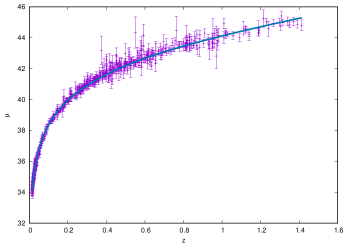
Figure 1: Apparent magnitude $\mu$ vs. redshift $z$ Hubble diagram from the Union 2.1 SNe Ia data (dots with their corresponding error bars) and the best fit from our model. The solid line represents the distance modulus $\mu(z)$ from the best fit to the data of the model.

The envelope curves that represent the statistical errors above and below the solid mean curve in Figure 1 have not been drawn since they turn out to be quite wide due to the somewhat large error in $n$.

With the mean values reported in Table 1, the Hubble constant $H_{0}$ given by equation (30) has the following numerical value:

$$H_{0}=66.95\,\mbox{km/s/Mpc},$$ (48)

which is in a great agreement with the value reported by Planck [69] (see Appendix B).

Due to limitations of the gnuplot’s fit routine and the divergences in the range $x<0$ of the $\Gamma(x)$ function, the convergence of the fit is highly dependent on the initial values of the free parameters $n$, $\gamma$ and $\Omega_{\text{M}}$. The results shown in Table 1 are obtained using a wide range of initial values. Another fit with a good convergence of the fit is given by the initial values: $n=1.3$, $\gamma=2.6$ and $\Omega_{\text{M}}=2.1$. The obtained values are reported in Table 2. The distance modulus-redshift plot for the values obtained in this fit is shown in Figure 2. The envelope curves that represent the statistical errors are present, but due to the small asymptotic errors such envelope is cover by the mean curve.

$\gamma$	$1.4937\pm 0.0003$
$\Omega_{\text{M}}$	$5.4220\pm 0.0243$
$n$	$0.5539\pm 0.0046$

	$\gamma$	$\Omega_{\text{M}}$	n
$\gamma$	1.000
$\Omega_{\text{M}}$	0.273	1.000
$n$	-0.140	0.587	1.000

Table 2: Left: Best fit results for the fractional derivative model with three free parameters: the fractional derivative order $\gamma$, the matter density parameter $\Omega_{\text{M}}$ and the power for the scale factor $n$ presented with their corresponding errors for the initial values: $n=1.3$, $\gamma=2.6$ and $\Omega_{\text{M}}=2.1$. The right panel shows the correlation matrix for the best fit values reported. The SSR and the $p$-value for this model are: $573.544$ and $0.50$ respectively

.

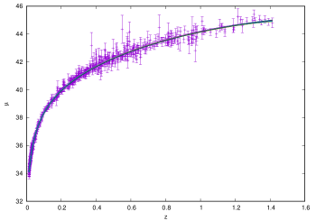
Figure 2: Apparent magnitude $\mu$ vs. redshift $z$ Hubble diagram from the Union 2.1 SNe Ia data (dots with their corresponding error bars) and the best fit from our model. The solid blue line represents the distance modulus $\mu(z)$ from the best fit to the data of the model. The other solid curves represents the envelope of the statistical errors.

For this set of initial values the resulting asymptotic error of the free parameters is considerably less than those reported in Table 1. The parameters $\gamma$ and $\Omega_{\text{M}}$ do not have a significant improvement, unlike the parameter $n$ whose error drastically decreased. Another relevant difference resides in the p-value, this statistical indicator increased, but is acceptable to within the ranges of gnuplot. With these results, the Hubble constant has the following value:

$$H_{0}=68.37\,\mbox{km/s/Mpc}.$$ (49)

VI Final remarks

In this article we have generalised the standard Friedmann equations of cosmology using fractional derivatives by performing a Last Step Modification approach. The obtained fractional Friedmann equations and the formulae of the corresponding fractional cosmographic parameters in terms of the cosmological density parameters were used to explain the current accelerated expansion of a dust and zero curvature Universe, without the introduction of a dark energy component. We introduced Milgrom’s acceleration constant into the built expressions with the intention of not requiring any non-baryonic dark matter component. The statistical fitting of the free parameters in the model shows an excellent agreement with a fractional derivative order of $3/2$, which has recently been shown to be the required fractional order to explain MOdified Newtonian Dynamics (MOND) phenomenology [76]. This result is in excellent agreements with the recent work by Barrientos, Bernal, and Mendoza [34] since the Universe at the present epoch is in the deep MOND regime. The introduction of fractional derivatives into physics usually means that non-locality is taking place at some level and it gets more noticeable at large scales. As noted by Barrientos, Bernal, and Mendoza [34], there are an infinite number of non-local relativistic theories of gravity with curvature-matter couplings that have MOND on their weak field limit of approximation. All this is pointing into the direction that MOND is most probably a non-local phenomenon which occurs at sufficiently small mass to squared length scales, i.e. at acceleration scales $\lesssim a_{0}$.

Strictly speaking, the fitting procedure is only giving information about the total matter density $\Omega_{\textrm{M}}$ which includes baryonic and non-baryonic components. In this sense the model presented shows that a simple introduction of fractional Friedmann equations in cosmology can account for a dark energy component. However, as mentioned in Section III, the introduction of Milgrom’s acceleration constant $a_{0}$ in equation (21) was done with the intention that the dark matter component would be taken into account by a MOND-like prescription. The obtained value of the fractional derivative order of $\sim 3/2$ in this article and the fact that we expect MONDian effects to be relevant in the present epoch dynamics of the Universe, further reinforce this result as mentioned in the previous paragraph.

The present work is restricted to a matter dominated Universe and puts aside the possibility of a dark-energy dominated Universe. The main reason lies in the complexity of the resultant equations. In fact, for a $\Lambda$-dominated Universe, equation (24) is not longer valid. Thinking in analogy to the standard cosmological model, we can expect that the scale factor for a dark-energy dominated era has an exponential dependence on $t$. However, the fractional derivative of an exponential function is a cumbersome expression that makes the fit extremely difficult. The case of a Universe where both components are taken into account is equally complex since our definitions for the cosmographic parameters require an equation for the Hubble parameter and equation (23) is a relation for $H^{\star}$. In order to have a more solid proposal, a more profound model needs to be built, introducing fractional derivatives in the principle of least action. Such topic goes beyond to the toy model introduced in this work.

The toy model presented in this article about the current expansion of the Universe using fractional derivatives using the Last Step Modification is to be taken with care. It represents a first exploration onto whether there could be any interesting aspects of gravitational theory to be more deeply investigated since the field equations do not come from a variational principle. We intend to go beyond the present work to construct a formalism in terms of fractional derivatives for geometrical objects in general relativity and in formulating a fractional calculus of variations with applications to gravitational theory.

Appendix A Fractional calculus: a simple introduction.

The question of whether it is possible to take half the derivative of a function goes back to a letter written by Leibniz to L’Hôpital in 1665. Since then the subject of fractional calculus, as it is now known, has attracted the interest of mathematicians like Abel, Liouville and Riemann, who developed the basis of the theory. In recent years, fractional derivatives have proved to be useful in many applications ranging from anomalous diffusion, finance to modeling of viscoelastic materials. As expected,when considering the order of differentiation to be an integer, the fractional derivative coincides with the standard definition. However, for non-integer values it has an intrinsic non-local character, which explains its applicability in complex phenomena in which long range interactions or memory effects are present. Before providing the general definition of fractional derivative, we give a few examples motivating this notion. Take for instance

$$f(x)=x^{k}.$$

Computing the first derivative we obtain

$$f^{\prime}(x)=\frac{df}{dx}=kx^{k-1}.$$

The successive repetition of this procedure $n$ times yields the $n$-th derivative:

$$\frac{d^{n}f}{dx^{n}}=\frac{k!}{(k-n)!}x^{k-n}.$$

The above expression makes perfect sense for a real number $k$, if we can define its factorial in a meaningful way. The $\Gamma$ function provides such a generalization, and the above expression can be written as

$$\frac{d^{\alpha}f}{dx^{\alpha}}=\frac{\Gamma(k+1)}{\Gamma(k-\alpha+1)}x^{k-\alpha},$$

where we have replaced $n$ by $\alpha$ to emphasize the fact that now the order of differentiation can be taken to be any real number.
A similar reasoning can be applied to other basic examples such as the exponential or trigonometric functions. In such a way, it is possible to define the fractional derivative or integral for functions expressed in their Taylor or Fourier series expansions. However, a more general and useful definition is based on the Riemann-Liouville representation formula of a function. More precisely, the integral operator of order $\alpha$ is defined as

$$I^{\alpha}f(t)=\frac{1}{\Gamma(\alpha)}\int_{0}^{t}\frac{f(\tau)}{(t-\tau)^{1-\alpha}}\,d\tau.$$

Again, this definition can be justified by applying the standard integral operator $m$ times and integrating by parts and then making sense of the definition for a real order of integration. Less intuitive, but more appropriate in formulating initial value problems than other definitions of fractional derivatives is the Caputo proposal given by

$$D^{\alpha}f(t)=I^{m-\alpha}D^{m}f=\frac{1}{\Gamma(m-\alpha)}\int_{0}^{t}(t-\tau)^{m-\alpha-1}f^{(m)}(\tau)\,d\tau,$$

for $m-1<\alpha<m$, $m\in\mathbb{N}$ and where $f^{(m)}$ denotes the standard derivative of $f$. For a systematic presentation of fractional calculus the reader is referred to Podlubny [44].

There are two properties of fractional derivatives that are important to mention since they depar from the common sense in ordinary calculus . The first one is the Leibniz’s rule for the product of two functions. Oldham and Spanier [80] proved that the most general expression is given by:

$$\frac{D^{\alpha}[fg]}{dx^{\alpha}}=\sum_{j=-\infty}^{\infty}\frac{\Gamma(\alpha+1)}{\Gamma(\alpha-\beta-j+1)\Gamma(\beta+j+1)}\frac{d^{\alpha-\beta-j}f}{dx^{\alpha-\beta-j}}\frac{d^{\beta+j}g}{dx^{\beta+j}}.$$

The second one is the composition rule:

$$D^{\alpha}D^{\beta}f=D^{\alpha+\beta}f-\sum_{k=0}^{\beta-1}\frac{[x-a]^{k-\alpha-\beta}f^{(k)}(a)}{\Gamma(k-\alpha-\beta+1)}.$$

Appendix B $\Lambda CDM$ standard cosmology.

With the intention of showing the robustness of the fitting procedure we are using in the article with the fit routine of gnuplot, we show in this appendix that for the case $\gamma=1$ we recover the values of $\Omega_{M}$ and $\Omega_{\Lambda}$ reported in the standard $\Lambda CDM$ cosmological model. To do so, we cannot simply fix the value $\gamma=1$ on all fractional equations since equation (27) is not valid for such value. Therefore, the non-fractional equations (6), (9), (14) and (18) must be employed. Unlike the fractional case, equation (6) is a constriction and not an equation for the Hubble parameter $H_{0}$. Since the distance modulus $\mu(z)$ relation (46) has an explicit dependence on this parameter, a value must be introduced. There are several values reported in the literature for $H_{0}$ that constitutes the so called “cosmological tension”. We performed fits to SN Ia data using the values reported by the Planck Collaboration [69]: $H_{0}^{\text{Planck}}=67.36\,\mbox{km s}^{-1}\mbox{Mpc}^{-1}$, a value from SN Ia observations: $H_{0}^{\text{SN\,Ia}}=63\,\mbox{km s}^{-1}\mbox{Mpc}^{-1}$ (see Fig. 9 in [73] and references therein) and a local Hubble constant [81]: $H_{0}^{\text{loc}}=75.35\,\mbox{km s}^{-1}\mbox{Mpc}^{-1}$.

Due to condition given by (6) the number of free parameters is reduced to one. $\Omega_{M}$ was chosen to be this free parameter. The results obtained by the fit are shown in Table 3.

	Planck	SN Ia	Local
$\Omega_{M}$	$0.185818$	$0.3601$	$0.027163$
Asymptotic Error	$\pm 0.008958$	$\pm 0.01343$	$\pm 0.005725$
SSR	$557.741$	$822.58$	$742.651$
p-value	$0.203964$	$<0.0001$	$<0.0001$

Table 3: Best fit results for the standard cosmological model with one free parameter: the matter density parameter $\Omega_{\text{M}}$, presented with its corresponding error, SSR and p-value.

The value of $\Omega_{M}^{\text{loc}}$ greatly differs from the standard estimation: $\Omega_{M}=0.27$. However, such value is between $\Omega_{M}^{Planck}$ and $\Omega_{M}^{SN\,Ia}$. Thus, a Hubble parameter $H_{0}$ between $63\,\mbox{km s}^{-1}\mbox{Mpc}^{-1}$ and $67.36\,\mbox{km s}^{-1}\mbox{Mpc}^{-1}$ will be closer to what is expected. A recent study made by Mukherjee et al. [82] reports the following estimations for the Hubble parameter and the matter density: $H_{0}=67.6^{+4.3}_{-4.2}\mbox{km s}^{-1}\mbox{Mpc}^{-1}$ and $\Omega_{M}=0.47^{+0.34}_{-0.27}$, which agree with the results obtained from our fit.

Figure 3 shows the Hubble diagram for the $\Lambda CDM$ cosmological model using the Planck value for the Hubble parameter.

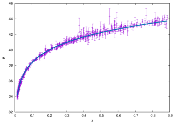
Figure 3: Apparent magnitude $\mu$ vs. redshift $z$ Hubble diagram from the Union 2.1 SN Ia data (dots with their corresponding error bars) and the best fit from the $\Lambda CDM$ cosmological model with $H_{0}^{\text{Planck}}=67.36\,\mbox{km s}^{-1}\mbox{Mpc}^{-1}$. The solid line represents the distance modulus $\mu(z)$ from the best fit to the data.

References

- Will [1993] C. M. Will, Theory and Experiment in Gravitational Physics, by Clifford M. Will, pp. 396. ISBN 0521439736. Cambridge, UK: Cambridge University Press, March 1993. (1993).
- Dyson, Eddington, and Davidson [1920] F. W. Dyson, A. S. Eddington, and C. Davidson, Philosophical Transactions of the Royal Society of London Series A 220, 291 (1920).
- Pound and Rebka [1960] R. V. Pound and G. A. Rebka, Phys. Rev. Lett. 4, 337 (1960).
- Reasenberg et al. [1979] R. D. Reasenberg, I. I. Shapiro, P. E. MacNeil, R. B. Goldstein, J. C. Breidenthal, J. P. Brenkle, D. L. Cain, T. M. Kaufman, T. A. Komarek, and A. I. Zygielbaum, ApJL 234, L219 (1979).
- Anderson et al. [1996] J. D. Anderson, M. Gross, K. L. Nordtvedt, and S. G. Turyshev, Astrophys. J. 459, 365 (1996), arXiv:gr-qc/9510029 [gr-qc] .
- Chandler et al. [2005] J. Chandler, M. Pearlman, R. Reasenberg, and J. Degnan, (2005).
- Ciufolini et al. [1998] I. Ciufolini, E. Pavlis, F. Chieppa, E. Fernandes-Vieira, and J. Perez-Mercader, Science 279, 2100 (1998).
- de Sitter [1916] W. de Sitter, MNRAS 77, 155 (1916).
- Eubanks et al. [1997] T. M. Eubanks, D. N. Matsakis, J. O. Martin, B. A. Archinal, D. D. McCarthy, S. A. Klioner, S. Shapiro, and I. I. Shapiro, in APS April Meeting Abstracts, APS Meeting Abstracts (1997) p. K11.05.
- Nordtvedt [1968] K. Nordtvedt, Physical Review 170, 1186 (1968).
- Nordtvedt [1973] K. Nordtvedt, Phys. Rev. D 7, 2347 (1973).
- Nordtvedt and Will [1972] J. Nordtvedt, Kenneth and C. M. Will, Astrophys. J. 177, 775 (1972).
- Schiff [1960] L. I. Schiff, Proceedings of the National Academy of Science 46, 871 (1960).
- Shapiro [1964] I. I. Shapiro, Phys. Rev. Lett. 13, 789 (1964).
- Mendoza [2015] S. Mendoza, Canadian Journal of Physics 93, 217 (2015).
- Starobinsky [1979] A. Starobinsky, JETP Lett. 30, 682 (1979).
- Nojiri and Odintsov [2011] S. Nojiri and S. D. Odintsov, Physics Reports 505, 59 (2011), arXiv:1011.0544 [gr-qc] .
- Nojiri and Odintsov [2008] S. Nojiri and S. D. Odintsov, Physics Letters B 659, 821 (2008), arXiv:0708.0924 [hep-th] .
- Shamir and Fayyaz [2020] M. F. Shamir and I. Fayyaz, Theoretical and Mathematical Physics 202, 112 (2020).
- Odintsov and Oikonomou [2020] S. D. Odintsov and V. K. Oikonomou, Physics Letters B 807, 135576 (2020), arXiv:2005.12804 [gr-qc] .
- Nojiri et al. [2020] S. Nojiri, S. D. Odintsov, V. K. Oikonomou, and A. A. Popov, Physics of the Dark Universe 28, 100514 (2020), arXiv:2002.10402 [gr-qc] .
- Nojiri and Odintsov [2004] S. Nojiri and S. D. Odintsov, General Relativity and Gravitation 36, 1765 (2004), arXiv:hep-th/0308176 [hep-th] .
- Nojiri and Odintsov [2003] S. Nojiri and S. D. Odintsov, Phys. Rev. D 68, 123512 (2003), arXiv:hep-th/0307288 [hep-th] .
- Harko and Lobo [2010] T. Harko and F. S. N. Lobo, European Physical Journal C 70, 373 (2010), arXiv:1008.4193 [gr-qc] .
- Harko et al. [2011] T. Harko, F. S. N. Lobo, S. Nojiri, and S. D. Odintsov, Phys. Rev. D 84, 024020 (2011), arXiv:1104.2669 [gr-qc] .
- Harko, Lobo, and Minazzoli [2013] T. Harko, F. S. N. Lobo, and O. Minazzoli, Phys. Rev. D 87, 047501 (2013), arXiv:1210.4218 [gr-qc] .
- Harko et al. [2014] T. Harko, F. S. N. Lobo, G. Otalora, and E. N. Saridakis, Phys. Rev. D 89, 124036 (2014), arXiv:1404.6212 [gr-qc] .
- Lobo and Harko [2012] F. S. N. Lobo and T. Harko, ArXiv e-prints (2012), arXiv:1211.0426 [gr-qc] .
- Bertolami et al. [2007] O. Bertolami, C. G. Böhmer, T. Harko, and F. S. N. Lobo, Phys. Rev. D 75, 104016 (2007), arXiv:0704.1733 [gr-qc] .
- Barrientos and Mendoza [2018] E. Barrientos and S. Mendoza, Phys. Rev. D 98, 084033 (2018), arXiv:1808.01386 [gr-qc] .
- Bernal et al. [2011a] T. Bernal, S. Capozziello, J. C. Hidalgo, and S. Mendoza, European Physical Journal C 71, 1794 (2011a), arXiv:1108.5588 [astro-ph.CO] .
- Mendoza et al. [2013] S. Mendoza, T. Bernal, X. Hernandez, J. C. Hidalgo, and L. A. Torres, MNRAS 433, 1802 (2013), arXiv:1208.6241 [astro-ph.CO] .
- Barrientos and Mendoza [2016] E. Barrientos and S. Mendoza, European Physical Journal Plus 131, 367 (2016), arXiv:1602.05644 [gr-qc] .
- Barrientos, Bernal, and Mendoza [2020] E. Barrientos, T. Bernal, and S. Mendoza, arXiv e-prints , arXiv:2008.01800 (2020), arXiv:2008.01800 [gr-qc] .
- Mashhoon [1993] B. Mashhoon, Phys. Rev. A 47, 4498 (1993).
- Mashhoon [2001] B. Mashhoon, arXiv e-prints , gr-qc/0112058 (2001), arXiv:gr-qc/0112058 [gr-qc] .
- Chicone and Mashhoon [2012] C. Chicone and B. Mashhoon, Journal of Mathematical Physics 53, 042501 (2012), arXiv:1111.4702 [gr-qc] .
- Chicone and Mashhoon [2016a] C. Chicone and B. Mashhoon, Classical and Quantum Gravity 33, 075005 (2016a), arXiv:1508.01508 [gr-qc] .
- Chicone and Mashhoon [2016b] C. Chicone and B. Mashhoon, Journal of Mathematical Physics 57, 072501 (2016b), arXiv:1510.07316 [gr-qc] .
- Blome et al. [2010] H.-J. Blome, C. Chicone, F. W. Hehl, and B. Mashhoon, Phys. Rev. D 81, 065020 (2010), arXiv:1002.1425 [gr-qc] .
- Maggiore and Mancarella [2014] M. Maggiore and M. Mancarella, Phys. Rev. D 90, 023005 (2014), arXiv:1402.0448 [hep-th] .
- Hehl and Mashhoon [2009] F. W. Hehl and B. Mashhoon, Physics Letters B 673, 279 (2009), arXiv:0812.1059 [gr-qc] .
- Foffa, Maggiore, and Mitsou [2014] S. Foffa, M. Maggiore, and E. Mitsou, International Journal of Modern Physics A 29, 1450116 (2014), arXiv:1311.3435 [hep-th] .
- Podlubny [1999] I. Podlubny, Fractional differential equations: an introduction to fractional derivatives, fractional differential equations, to methods of their solution and some of their applications, Mathematics in Science and Engineering (Academic Press, London, 1999).
- Kochubei and Luchko [2019a] A. Kochubei and Y. Luchko, Basic Theory (De Gruyter, Berlin, Boston, 19 Feb. 2019).
- Kochubei and Luchko [2019b] A. Kochubei and Y. Luchko, Fractional Differential Equations (De Gruyter, Berlin, Boston, 19 Feb. 2019).
- Karniadakis [2019] G. E. Karniadakis, Numerical Methods (De Gruyter, Berlin, Boston, 15 Apr. 2019).
- Tarasov [2019] V. E. Tarasov, Applications in Physics, Part A (De Gruyter, Berlin, Boston, 19 Feb. 2019).
- Petráš [2019] I. Petráš, Applications in Control (De Gruyter, Berlin, Boston, 19 Feb. 2019).
- Bǎleanu and Lopes [2019] D. Bǎleanu and A. M. Lopes, Applications in Engineering, Life and Social Sciences, Part A (De Gruyter, Berlin, Boston, 01 Apr. 2019).
- Shchigolev [2011] V. K. Shchigolev, Communications in Theoretical Physics 56, 389 (2011), arXiv:1011.3304 [gr-qc] .
- Shchigolev [2013a] V. K. Shchigolev, Discontinuitynlinearity and Complexity 2, 115 (2013a), arXiv:1208.3454 [gr-qc] .
- Shchigolev [2016] V. K. Shchigolev, European Physical Journal Plus 131, 256 (2016), arXiv:1512.04113 [gr-qc] .
- Shchigolev [2013b] V. K. Shchigolev, Modern Physics Letters A 28, 1350056 (2013b), arXiv:1301.7198 [gr-qc] .
- Roberts [2009] M. D. Roberts, arXiv e-prints , arXiv:0909.1171 (2009), arXiv:0909.1171 [gr-qc] .
- Vacaru [2012] S. I. Vacaru, International Journal of Theoretical Physics 51, 1338 (2012), arXiv:1004.0628 [math-ph] .
- Rami [2005] E.-N. A. Rami, Electronic Journal of Theoretical Physics 2, 1 (2005).
- Frederico and Torres [2006] G. S. F. Frederico and D. F. M. Torres, arXiv Mathematics e-prints , math/0607472 (2006), arXiv:math/0607472 [math.OC] .
- Baleanu [2007] D. Baleanu, Proceedings in Applied Mathematics and Mechanics 7 (2007), 10.1002/pamm.200700327.
- El-Nabulsi and Torres [2008] R. A. El-Nabulsi and D. F. M. Torres, Journal of Mathematical Physics 49, 053521 (2008), arXiv:0804.4500 [math-ph] .
- Herzallah and Baleanu [2009] M. Herzallah and D. Baleanu, Nonlinear Dynamics 58, 385 (2009).
- Baleanu and Muslih [2005] D. Baleanu and S. I. Muslih, Physica Scripta 72, 119 (2005).
- El-Nabulsi [2013] R. El-Nabulsi, Nonlinear Dynamics 74 (2013), 10.1007/s11071-013-0977-6.
- Peacock [1999] J. A. Peacock, Cosmological Physics (1999).
- Misner, Thorne, and Wheeler [1973] C. W. Misner, K. S. Thorne, and J. A. Wheeler, Gravitation (1973).
- Longair [1989] M. S. Longair, “Galaxy Formation,” in Evolution of Galaxies: Astronomical Observations, Vol. 333, edited by I. Appenzeller, H. J. Habing, and P. Lena (1989) p. 1.
- Peebles [1993] P. J. E. Peebles, Principles of Physical Cosmology (1993).
- Li, Du, and Xu [2020] E.-K. Li, M. Du, and L. Xu, MNRAS 491, 4960 (2020), arXiv:1903.11433 [astro-ph.CO] .
- Planck Collaboration et al. [2018] Planck Collaboration, N. Aghanim, Y. Akrami, M. Ashdown, J. Aumont, C. Baccigalupi, M. Ballardini, A. J. Banday, R. B. Barreiro, N. Bartolo, S. Basak, R. Battye, K. Benabed, J. P. Bernard, M. Bersanelli, P. Bielewicz, J. J. Bock, J. R. Bond, J. Borrill, F. R. Bouchet, F. Boulanger, M. Bucher, C. Burigana, R. C. Butler, E. Calabrese, J. F. Cardoso, J. Carron, A. Challinor, H. C. Chiang, J. Chluba, L. P. L. Colombo, C. Combet, D. Contreras, B. P. Crill, F. Cuttaia, P. de Bernardis, G. de Zotti, J. Delabrouille, J. M. Delouis, E. Di Valentino, J. M. Diego, O. Doré, M. Douspis, A. Ducout, X. Dupac, S. Dusini, G. Efstathiou, F. Elsner, T. A. Enßlin, H. K. Eriksen, Y. Fantaye, M. Farhang, J. Fergusson, R. Fernandez-Cobos, F. Finelli, F. Forastieri, M. Frailis, A. A. Fraisse, E. Franceschi, A. Frolov, S. Galeotta, S. Galli, K. Ganga, R. T. Génova-Santos, M. Gerbino, T. Ghosh, J. González-Nuevo, K. M. Górski, S. Gratton, A. Gruppuso, J. E. Gudmundsson, J. Hamann, W. Handley, F. K. Hansen, D. Herranz, S. R. Hildebrandt, E. Hivon, Z. Huang, A. H. Jaffe, W. C. Jones, A. Karakci, E. Keihänen, R. Keskitalo, K. Kiiveri, J. Kim, T. S. Kisner, L. Knox, N. Krachmalnicoff, M. Kunz, H. Kurki-Suonio, G. Lagache, J. M. Lamarre, A. Lasenby, M. Lattanzi, C. R. Lawrence, M. Le Jeune, P. Lemos, J. Lesgourgues, F. Levrier, A. Lewis, M. Liguori, P. B. Lilje, M. Lilley, V. Lindholm, M. López-Caniego, P. M. Lubin, Y. Z. Ma, J. F. Macías-Pérez, G. Maggio, D. Maino, N. Mandolesi, A. Mangilli, A. Marcos-Caballero, M. Maris, P. G. Martin, M. Martinelli, E. Martínez-González, S. Matarrese, N. Mauri, J. D. McEwen, P. R. Meinhold, A. Melchiorri, A. Mennella, M. Migliaccio, M. Millea, S. Mitra, M. A. Miville-Deschênes, D. Molinari, L. Montier, G. Morgante, A. Moss, P. Natoli, H. U. Nørgaard-Nielsen, L. Pagano, D. Paoletti, B. Partridge, G. Patanchon, H. V. Peiris, F. Perrotta, V. Pettorino, F. Piacentini, L. Polastri, G. Polenta, J. L. Puget, J. P. Rachen, M. Reinecke, M. Remazeilles, A. Renzi, G. Rocha, C. Rosset, G. Roudier, J. A. Rubiño-Martín, B. Ruiz-Granados, L. Salvati, M. Sandri, M. Savelainen, D. Scott, E. P. S. Shellard, C. Sirignano, G. Sirri, L. D. Spencer, R. Sunyaev, A. S. Suur-Uski, J. A. Tauber, D. Tavagnacco, M. Tenti, L. Toffolatti, M. Tomasi, T. Trombetti, L. Valenziano, J. Valiviita, B. Van Tent, L. Vibert, P. Vielva, F. Villa, N. Vittorio, B. D. Wand elt, I. K. Wehus, M. White, S. D. M. White, A. Zacchei, and A. Zonca, arXiv e-prints , arXiv:1807.06209 (2018), arXiv:1807.06209 [astro-ph.CO] .
- Sedov [1959] L. I. Sedov, Similarity and Dimensional Methods in Mechanics, New York: Academic Press, 1959 (1959).
- Liddle [2013] A. Liddle, An Introduction to Modern Cosmology (Wiley, 2013).
- Dodelson and 1941-1969). [2003] S. Dodelson and A. P. L. . 1941-1969)., Modern Cosmology (Elsevier Science, 2003).
- Perlmutter et al. [1999] S. Perlmutter, G. Aldering, G. Goldhaber, R. A. Knop, P. Nugent, P. G. Castro, S. Deustua, S. Fabbro, A. Goobar, D. E. Groom, I. M. Hook, A. G. Kim, M. Y. Kim, J. C. Lee, N. J. Nunes, R. Pain, C. R. Pennypacker, R. Quimby, C. Lidman, R. S. Ellis, M. Irwin, R. G. McMahon, P. Ruiz-Lapuente, N. Walton, B. Schaefer, B. J. Boyle, A. V. Filippenko, T. Matheson, A. S. Fruchter, N. Panagia, H. J. M. Newberg, W. J. Couch, and T. S. C. Project, Astrophys. J. 517, 565 (1999), arXiv:astro-ph/9812133 [astro-ph] .
- Visser [2005] M. Visser, Gen. Rel. Grav. 37, 1541 (2005), arXiv:gr-qc/0411131 .
- Suzuki et al. [2012] N. Suzuki, D. Rubin, C. Lidman, G. Aldering, R. Amanullah, K. Barbary, L. F. Barrientos, J. Botyanszki, M. Brodwin, N. Connolly, K. S. Dawson, A. Dey, M. Doi, M. Donahue, S. Deustua, P. Eisenhardt, E. Ellingson, L. Faccioli, V. Fadeyev, H. K. Fakhouri, A. S. Fruchter, D. G. Gilbank, M. D. Gladders, G. Goldhaber, A. H. Gonzalez, A. Goobar, A. Gude, T. Hattori, H. Hoekstra, E. Hsiao, X. Huang, Y. Ihara, M. J. Jee, D. Johnston, N. Kashikawa, B. Koester, K. Konishi, M. Kowalski, E. V. Linder, L. Lubin, J. Melbourne, J. Meyers, T. Morokuma, F. Munshi, C. Mullis, T. Oda, N. Panagia, S. Perlmutter, M. Postman, T. Pritchard, J. Rhodes, P. Ripoche, P. Rosati, D. J. Schlegel, A. Spadafora, S. A. Stanford, V. Stanishev, D. Stern, M. Strovink, N. Takanashi, K. Tokita, M. Wagner, L. Wang, N. Yasuda, H. K. C. Yee, and T. Supernova Cosmology Project, Astrophys. J. 746, 85 (2012), arXiv:1105.3470 [astro-ph.CO] .
- Giusti [2020] A. Giusti, Phys. Rev. D 101, 124029 (2020), arXiv:2002.07133 [gr-qc] .
- Milgrom [1983] M. Milgrom, Astrophys. J. 270, 365 (1983).
- Milgrom [2008] M. Milgrom, arXiv e-prints , arXiv:0801.3133 (2008), arXiv:0801.3133 [astro-ph] .
- Bernal et al. [2011b] T. Bernal, S. Capozziello, G. Cristofano, and M. de Laurentis, Modern Physics Letters A 26, 2677 (2011b), arXiv:1110.2580 [gr-qc] .
- Oldham and Spanier [2006] K. Oldham and J. Spanier, The Fractional Calculus: Theory and Applications of Differentiation and Integration to Arbitrary Order, Dover books on mathematics (Dover Publications, 2006).
- Camarena and Marra [2020] D. Camarena and V. Marra, Phys. Rev. Research 2, 013028 (2020).
- Mukherjee et al. [2020] S. Mukherjee, A. Ghosh, M. J. Graham, C. Karathanasis, M. M. Kasliwal, I. Magaña Hernandez, S. M. Nissanke, A. Silvestri, and B. D. Wandelt, arXiv e-prints , arXiv:2009.14199 (2020), arXiv:2009.14199 [astro-ph.CO] .