Non–relativistic Boson Stars as N–Body Quantum Systems

Abstract

In the present work, we analyze the structural configuration of a collection of generic non–relativistic bosons forming a gravitational bound Bose–Einstein condensate that we interpreted as a non–relativistic boson star. We prove that the system’s behavior can be obtained by analyzing its fundamental constituent’s properties, i.e., the single particle properties. Additionally, we show that by expressing the corresponding Newtonian gravitational potential, under certain circumstances, as a harmonic oscillator potential ones, we can describe the conditions in which the non–relativistic boson star can form equilibrium configurations. In order to analyze the structural configuration related to the boson star, we employ four different ansätze commonly used in the literature. The use of these ansätze allows to compare the structural properties of the bosonic cloud or the boson star that leads to obtain several equilibrium configurations from compact objets matching to the size of typical stars to very gigantic systems comparable to the size of galaxy cluster dark matter halos. Finally, we show that these ansätze predict, qualitatively speaking, the same structural and gravitational equilibrium configurations for different values of the parameters involved.

I Introduction

Bose–Einstein condensates (BECs) play a very exciting and essential role in modern physics, relating a multitude of models spreading from microscopic well proved behavior of ultra–cold quantum gases to galactic and cosmological scales. Nevertheless, there is an issue not well understood in this scenario which deserves more in-depth study, i.e., the non–trivial conditions in which scalar fields can form BECs B1 ; B2 ; B3 ; B4 ; B5 ; B6 ; B7 ; Nos . However, it seems to be that scalar fields in the form of some type of BEC formed by generic bosons can describe the basic properties of dark matter (DM) in the universe DM ; DM1 ; DM2 ; DM3 ; DM4 ; DM5 ; DM6 . According to this line of thought, DM consists of a certain type of spin–zero bosons, such as ultra-light scalar field dark matter or fuzzy dark matter, weakly interacting massive particles, axions, etc., (depending on the specific model under consideration) which have not yet been observed. The bosonic character of these particles, using the theory of relativistic Bose gases JB ; LP , also opens the door for the existence of scalar field dark matter in the form of BECs BoehmerHarko2007 ; ure .
Complementary to the ideas mentioned above, some particular theoretical objects can be formed in a very similar manner. In some circumstances, a system of generic bosons can form gravitationally bound BECs leading to macroscopic objects, the so–called boson stars (BSs) 1 ; 2 ; 3 . On the one hand, some research lines suggest that BSs could be alternative candidates for black holes in the center of galaxies. On the other hand, it is generally accepted that the fundamental constituents of BSs are some generic scalars in the form of some type of BEC Eckehard . This last assertion opens up the opportunity to describe these objects with BEC’s formalism, which enriches the analysis. We must mention that the study of BSs and its interpretation as BECs has been extensively analyzed SL . Although these objects have also not been observed yet, their behavior and their structural properties lead us to think that these systems are highly related to scalar dark matter clouds in the universe. There is a zoo of these objects (BSs) in the literature Eckehard , basically characterized according to its dynamical behavior. For instance, BS could lie in the relativistic regime or not, they can also be characterized with respect to the type of self–interactions within the system Eckehard , etc. The structural properties of the BS are quite interesting. For instance, Heisenberg’s Uncertainty Principle provides pressure support in order to get a stable object. The size of the BS ranges from giant to very compact objects depending on the nature of the involved functional interactions among the constituents of the system. Finally, we must mention that the Klein–Gordon equation coupled with gravity describes the dynamics of BSs in the relativistic regime, and consequently, some Gross–Pitaevskii like–equations also coupled with gravity describe the dynamics in the non–relativistic limit, the so–called Gross–Pitaevskii–Poisson equation, see for instance Kling1 ; Kling2 and references therein. It is quite interesting that the non–relativistic limit of the self–interacting Klein–Gordon equation, which describes the dynamics of BSs, leads to the so–called Gross–Pitaevskii equation, when the scalar potential is of the form $m^{2}|\phi|^{2}+\lambda|\phi|^{4}$, being $m$ the mass parameter and $\lambda$ the term related to self–interactions. Clearly, more general forms of the Gross–Pitaevskii equation can be used to generalize the corresponding interactions within the system. Those mentioned earlier lead to criteria of structural characterization of the BS, for instance, its size, stability, etc., by using (under certain conditions) the basic formalism behind usual laboratory BECs. Strictly speaking, the Gross–Pitaevskii equation is an approximated equation valid for systems at zero temperature. Nevertheless, the predictions made by the Gross–Pitaevskii equation are a good approximation for temperatures $T<T_{c}$, where $T_{c}$ is the condensation temperature of the system. Such an equation can be used to analyze diluted weakly interacting systems’ properties and when the number of particles is large enough for the condensed phase. However, when the corresponding Gross–Pitaevskii–Poisson equation is used to study the structural properties of the BS, the N–particles that constitute the system are analyzed as a single particle(–field). In other words, the nature of the phase transition provides the advantage to reduce the analysis of the $N$-body system to the analysis of the dynamics of a single body(–field) as in usual BECs. For this reason, we call the field appearing in the Gross–Pitaevskii–Poisson equation the order parameter. The order parameter contains the information of the N–particles forming the condensed phase, and due to the highly correlated behavior of the BEC, this system behaves as a single entity.
In this work, we assume from the very beginning that the non–relativistic behavior of the BS can be described as a collection of weakly interacting generic bosons that are able to form gravitationally bound BECs. In other words, we describe some structural properties related to the BS through the quantum properties of its basic constituents, i.e., the properties of a single particle.
The paper is organized as follows. In section II, we study the fundamental properties of the BS viewed as a collection of bosons starting from the single particle description. We assume that the system behaves as a BEC. Also, we describe the approximation in which the Newtonian gravitational potential can be expressed as a harmonic oscillator potential that we interpreted as the trapping potential, like in usual laboratory BECs. In section III, we analyze the relevant structural functions that characterize the ground state of the system to obtain criteria of stability upon the BS. Finally, in section V, we present a discussion, conclusions, and outlook.

II N–Body Quantum System as a Non–Relativistic Boson Star

As was mentioned in the introduction, the basic constituents of BSs are scalar particles(–field) (or spin zero–bosons), probably in the form of a BEC. In this section we analyze the non–relativistic BSs behavior as a collection of bosons interpreted as a quantum $N$–body system, in order to analyze some relevant properties associated with the bosonic cloud viewed as a BEC. In this aim, we define the following $N$–body Hamiltonian which describes our non–relativistic BS

$$\hat{H} = -\frac{\hbar^{2}}{2m_{\phi}}\sum_{\delta,\gamma}\langle\delta|\nabla^{2}|\gamma\rangle\hat{a}^{{\dagger}}_{\delta}\hat{a}_{\gamma}$$

$$+ \frac{1}{2}\sum_{\delta,\gamma,\mu,\nu}\langle\delta,\gamma|V_{int}|\mu,\nu\rangle\hat{a}^{{\dagger}}_{\delta}\hat{a}_{\gamma}\hat{a}^{{\dagger}}_{\mu}\hat{a}_{\nu}$$

$$+ \sum_{\delta,\gamma}\langle\delta|V_{g}|\gamma\rangle\hat{a}^{{\dagger}}_{\delta}\hat{a}_{\gamma}$$

where $m_{\phi}$ is the mass of the boson particle and $V_{int}$ is the potential which describe the interactions within the system. Moreover, we have also inserted in Eq. (II) the contributions of the gravitational potential $V_{g}$. Additionally, the operators $\hat{a}$ and $\hat{a}^{\dagger}$, correspond to the creation and annihilation operators for bosons, satisfying the usual canonical commutation relations

$$[\hat{a}_{\mu},\hat{a}_{\nu}^{\dagger}]=\delta_{\mu\nu},\,\,\,\ [\hat{a}_{\mu},\hat{a}_{\nu}]=[\hat{a}_{\mu}^{\dagger},\hat{a}_{\nu}^{\dagger}]=0.$$ (2)

As was mentioned above, the term, $V_{int}$ denotes the inter–particle potential, that will be assumed as $V_{int}\equiv U_{0}=\frac{4\pi\hbar^{2}}{m_{\phi}}a$, with $a$ the s–wave scattering length, i.e., at temperatures below the condensation temperature, only two–body interactions are taken into account. In other words, the system is diluted enough, and fulfills the condition $\rho|a|^{3}\ll 1$, where $\rho$ is the density of particles Dalfovo ; Ueda ; Pitaevski ; Pethick . Additionally, $V_{g}$ depicts the contributions of the gravitational potential within the BS that we assume for simplicity with spherical symmetry.

Notice that in the corresponding $N$–body Hamiltonian Eq. (II) we have the following terms

$$\langle\delta|{\nabla}^{2}|\gamma\rangle=\int{d}^{3}r{u}_{\delta}^{*}(\vec{r}){\nabla}^{2}{u}_{\gamma}(\vec{r}),$$ (3)

$$\langle\delta,\gamma|V_{int}|\mu,\nu\rangle=$$ (4)

$$\int\int{d}^{3}{r}_{1}{d}^{3}{r}_{2}{u}_{\delta}^{*}(\vec{r}_{1}){u}_{\gamma}^{*}(\vec{r}_{2})U_{0}{u}_{\mu}(\vec{r}_{2}){u}_{\nu}(\vec{r}_{1}),$$

$$\langle\delta|V_{g}|\gamma\rangle=\int{d}^{3}r{u}_{\delta}^{*}(\vec{r})V_{g}{u}_{\gamma}(\vec{r}),$$ (5)

where $\{{u}_{\gamma}(\vec{r})\}$ is a set of single–particle functions.

Although the mean field solutions for the gravitational potential with no interactions, are known in terms of hypergemoeometric functions, one can in principle, introduce some approximation to the gravitational potential. Let us consider a test particle in the outermost layer of the star, then its gravitational potential energy is proportional to the product of its masses, by the inverse of the distance to the center of the star that concentrates the largest part of the mass. For a spherically symmetric distribution, the first approximation is such that the mass is proportional to the central density times the volume of the sphere. Then, the gravitational potential would be proportional to the distance squared, i.e., a harmonic potential. This approximation is made precise in Refs. Abel ; Abel1 .

First, let us recall that the mass $M_{T}$ within a spherically symmetric BS, is given by

$$M_{T}(r)=4\pi\,m_{\phi}N\int_{0}^{r}\rho(r^{\prime})\,{r^{\prime}}^{2}\,dr^{\prime}.$$ (6)

where $0\leqslant r\leqslant R$. The radius $R$ will be considered the radius of the BS if most of its mass is contained in a region bounded by that radius. $N$ is the corresponding number of particles and $\rho(r)$ is the one particle probability density, which admits a series expansion when most of the matter of the BS is close enough to $r=0$, i.e.,

$$\rho(r)=\rho(r=0)+\sum_{n=1}^{\infty}\frac{\rho^{(n)}(r=0)r^{n}}{n\,!},$$ (7)

where $m_{\phi}N\rho(r=0)$ is the central mass density of the BS, and $\rho^{(n)}$ its corresponding derivatives. However, the density $\rho(r)$ tends to infinity as $r\rightarrow\infty$ which is a non physical behavior since the density $\rho(r)$ must tends zero for large $r$. In order to avoid this unphysical scenario it is assumed that

$$\Bigg{|}\frac{\rho^{(n)}(r=0)}{\rho(r=0)}\Bigg{|}\approx\frac{1}{R^{n}}.$$ (8)

Now, for the motion of a test particle that goes through the BS along the collinear diameter with the $z$-axis, the density peak is at the center of the BS, yielding

$$M_{T}(r)=\frac{4}{3}\pi\,m_{\phi}N\rho(r=0)r^{3}\Bigg{[}1+3\sum_{n=2}^{\infty}\frac{1}{(n+3)n\,!}\Bigl{(}\frac{r}{R}\Bigr{)}^{n}\Bigg{]}.$$ (9)

The sum in Eq. (9) must be convergent, but small by hypothesis. Indeed, in Ref. Abel , it is shown that $\forall\delta$ there is an index of the sum such that, for all the terms greater than that corresponding to such index, the sum is bounded by $\delta$. For $\delta$ small enough but not negligible, the remaining terms of the sum can be considered as perturbations. Therefore, the main term of the potential is reduced to a harmonic potential with an effective gravitational frequency given by

$$\omega_{g}=\sqrt{\alpha\pi Gm_{\phi}N\rho(r=0)},$$ (10)

where $G$ is the Newtonian constant of gravitation. Here also $\alpha=4/3+4\delta$. If $\delta=10^{-1}$, corresponding to less than 10 % of the total mass, the factor $52/30$ of Ref. Abel is recovered. Briefly, we can define an effective gravitational frequency, so that the gravitational potential can be interpreted at first order, as a trapping harmonic–like potential, as occurs in the usual BEC’s formalism.

III Boson Star Structural Analysis

According to the conditions obtained in the previous section, the corresponding analysis for the properties related to the BS can be summarized as follows, the trapping potential is given by

$$V_{g}\approx\frac{1}{2}m_{\phi}\omega_{g}^{2}r^{2},$$ (11)

and the approximation for the total mass

$$M_{T}\approx 4\pi\,Nm_{\phi}\int_{0}^{R}\rho(r=0)\,r^{2}\,dr.$$ (12)

On the other hand, if we further assume that most of the particles are inside the condensate, that is, in the $\vec{p}=0$ state then, this implies that the number of particles in the excited states is negligible for temperatures $T<T_{c}$, where $T_{c}$ is the condensation temperature. The contributions of the particles in the excited states could affect the properties of the system, see for instance Ref. Abel . However, we consider here that almost all the particles lies in the corresponding ground state according to the approximation Eq. (13). The contributions of the excited states could be important in the stability analysis and will be analyzed in future works. Thus, the last assertions can be expressed as follows.

$$N_{0}\approx N,\hskip 14.22636pt\sum_{\vec{p}\not=0}N_{\vec{p}}\ll N,$$ (13)

being $N$ the total number of particles, $N_{\vec{p}}$ the number of particles in the excited states, and $N_{0}$ the number of particles in the ground state. Keeping terms up to second order in $\hat{a}_{0}$ and $\hat{a}^{{\dagger}}_{0}$, i.e., $\langle\hat{a}_{0}^{{\dagger}}\hat{a}_{0}\rangle=\langle N\rangle$, we are able to obtain the ground state energy ($E_{0}$) associated with our BS

$$E_{0} = -\frac{{\hbar}^{2}}{2m_{\phi}}\langle 0|\nabla^{2}|0\rangle N+\frac{1}{2}\langle 0,0|U_{0}|0,0\rangle{N}^{2}$$

$$+ \langle 0|V_{g}|0\rangle N$$

Thus, we have for instance for the kinetic energy

$$\langle 0|\nabla^{2}|0\rangle=\int_{0}^{\infty}\int_{\Omega}\Psi_{0}^{*}(r)\nabla^{2}\Psi_{0}(r){r}^{2}\sin\theta drd\theta d\phi,\,\,\,\,$$ (15)

and so on for each of the energy contributions to the ground state Eq. (III).

G E LE C $\Psi_{0}(r)$ ${\Bigl{(}\frac{{\beta}^{2}}{\pi}\Bigr{)}}^{3/4}{e}^{-{\beta}^{2}{r}^{2}/2}$ ${\Bigl{(}\frac{{\beta}^{2}}{\pi^{2/3}}\Bigr{)}}^{3/4}{e}^{-{\beta}r}$ ${\Bigl{(}\frac{{\beta}^{2}}{7^{2/3}\pi^{2}}\Bigr{)}}^{3/4}\left(1+r\beta\right){e}^{-{\beta}r}$ $\sqrt{\frac{4\pi\beta^{3}}{(2\pi^{2}-15)}}\cos^{2}\left(\frac{\pi\beta r}{2}\right)$ A $\pi^{-3/2}$ $\pi^{-1}$ $\frac{1}{7\pi^{3}}$ $\frac{4\pi}{(2\pi^{2}-15)}$ $\kappa$ $2.8$ $4.2$ $5.4$ $1$ $\epsilon_{1}$ $\frac{3}{4}$ $\frac{1}{2}$ $\frac{3}{14\pi^{2}}$ $\frac{(4\pi^{2}-6)\pi^{2}}{(24\pi^{2}-180)}$ $\epsilon_{2}$ $\frac{3}{4}$ $\frac{1}{2}$ $\frac{81}{28\pi^{2}}$ $\frac{3(2\pi^{4}-5\pi^{2}+315)}{10(2\pi^{3}-15\pi)}$ $\epsilon_{3}$ $\frac{1}{2(2\pi)^{3/2}}$ $\frac{1}{16\pi}$ $\frac{437}{25088\pi^{5}}$ $\frac{35(24\pi^{3}-205\pi)}{288(2\pi^{2}-15)}$

Table 1: Ansätze table for the wave function of a single particle and its corresponding parameters $A,\kappa,\epsilon_{1},\epsilon_{3},\epsilon_{3}$. The ansätze presented here are known in the literature as the Gaussian (G), exponential (E), the linear exponential (LE) and the compact (C), respectively.

At this point, we introduce some well–known ansätze for the single-particle wave function $\Psi_{0}(r)$, which are summarized in the Table 1. There are several ansätze used in the literature. As the wave functions for BS usually do not have compact support, three non–compact ansätze are proposed, see for instance Ref. Joshua and references therein. However, in the Thomas–Fermi approximation, the BS can have a fixed radius, which may have some advantages Joshua1 , for which we also propose a compact ansatz. Sometimes, these functions contain adjustable parameters to compare with the numerical solutions Joshua . As we see in the Table 1, each of our proposed wave function has a single parameter $\beta$ with units of the inverse of length. In principle, this parameter can be different in each case, but due to the approximation of the harmonic potential, we will assume that it fulfills ${\beta}=\sqrt{\frac{m_{\phi}\omega_{g}}{\hbar}}$. Moreover, as we will see later in the manuscript, its meaning is related to the BS’s radius.

On the other hand, the probability density is the square of the wave function, $\rho(r)=|\Psi_{0}(r)|^{2}$. From this definition, we can obtain the corresponding central density evaluating at $r=0$, i. e.

$$\rho(r=0)=A\,\beta^{3},$$ (16)

where $A$ is a numerical factor that depends on whether it is Gaussian (G), Exponential (E), Linear–Exponential (LE), or Compact (C) anzatz, according to table 1. Notice that the central density in each case is expressed in terms of the parameter $\beta$. We can substitute these central densities in the expression for the effective gravitational frequency Eq. (10) that gives us

$$\omega_{g}=\sqrt{\alpha\pi AGm_{\phi}N\beta^{3}},$$ (17)

also in terms of the inverse length $\beta$.

Let us realize that $\beta$ depends on the effective gravitational frequency, and this, in turn, depends on the central density, i.e., by using Eq. (16) we obtain

$$\rho(r=0) = A\beta^{3}=A\left(\frac{m_{\phi}\omega_{g}}{\hbar}\right)^{3/2}$$

$$= A\left(\frac{m_{\phi}}{\hbar}\right)^{3/2}\left(\alpha G\pi m_{\phi}N\rho(r=0)\right)^{3/4}.$$

Therefore, if the ansätze given in Table 1 and the potential Eq. (11) be compatible, then the following expression for the central density of the BS must be consistent

$$\rho(r=0)=\left(\alpha G\pi\frac{m_{\phi}^{3}}{\hbar^{2}}\right)^{3}A^{4}N^{3}.$$ (19)

Notice that for all practical purposes the effective gravitational frequency for each ansatz has the same functional form, qualitatively speaking, and consequently the functional form of the central density for each ansatz has this shape.

On the other hand, with the expression for $\beta$ in terms of the effective gravitational frequency, if we substitute $\omega_{g}$ form Eq. (10), and central density from Eq. (19), we obtain an order of magnitude for the inverse length parameter $\beta$ for each ansätze, as follows

$$\beta=\frac{\alpha\pi GAN}{\hbar^{2}}m_{\phi}^{3}.$$ (20)

Although this characteristic length is not precisely the BS’s radius, it gives us an estimate of its size. Indeed, the ratio between the BS radius and this length is a fixed quantity $R\beta=\kappa$ that depends on the chosen ansatz Joshua as shown in table 1 . In the case of the compact ansatz, the radius can be considered as the inverse of the $\beta$ parameter, $R=\beta^{-1}$.

Let us calculate the corresponding ground state energy of the BS, by substituting each ansätze into the ground state energy Eq. (III), to obtain the following expression

$$E_{0}=\epsilon_{1}\frac{{\hbar}^{2}\beta^{2}N}{m_{\phi}}+\epsilon_{2}\frac{m_{\phi}\omega_{g}^{2}N}{\beta^{2}}+\epsilon_{3}U_{0}\beta^{3}N^{2},$$ (21)

where the numerical coefficients $\epsilon_{i}$ differ for each ansätze and are also shown in Table 1. Note that the radial integral in Eq. (III) cannot be performed up to infinity for the compact ansatz case, since one need to ask that the function vanishes for radii greater than $\beta^{-1}$. In other circumstances, it is known that this can lead to some difficulties Joshua . However, in this case, it is enough to integrate up to $\beta^{-1}$ to obtain the numerical coefficients above.

To obtain the thermodynamic quantities, it will be necessary to replace $\beta$ and $\omega_{g}$ as functions of the volume. Since we are considering a spherically symmetric BS, the available volume in the ideal case, i.e., when the interactions among the constituents within the BS are neglected, is as follows $V_{BS}=4\pi\kappa^{3}\beta^{-3}/3$, so ground state energy becomes

$$E_{0} = \epsilon_{1}\frac{{\hbar}^{2}N}{m_{\phi}}\left(\frac{4\pi\kappa^{3}}{3}\right)^{2/3}V_{BS}^{-2/3}$$

$$+ \epsilon_{2}\pi A\alpha Gm_{\phi}^{2}N^{2}\left(\frac{4\pi\kappa^{3}}{3}\right)^{1/3}V_{BS}^{-1/3}$$

$$+ \epsilon_{3}U_{0}N^{2}\left(\frac{4\pi\kappa^{3}}{3}\right)V_{BS}^{-1},$$

From the $N$–body ground state energy Eq. (III) we therefore calculate the ground state pressure $P_{0}=-\frac{\partial E_{0}}{\partial V_{BS}}$ for each ansätze with the result

$$P_{0} = \left(\frac{3}{4\pi\kappa^{3}}\right)\Bigl{[}\frac{2}{3}\epsilon_{1}\frac{\hbar^{2}N}{m_{\phi}}\beta^{5}$$

$$+ \frac{1}{3}\epsilon_{2}\pi A\alpha Gm_{\phi}^{2}N^{2}\beta^{4}+\epsilon_{3}U_{0}N^{2}\beta^{6}\Bigr{]}.$$

After rearranging the terms by identifying the scale $\beta$ from Eq. (20), we can obtain the following two terms, which are of the same order in the length scale that those usually found, but with different coefficients

$$P_{0} = \left(\frac{3}{4\pi\kappa^{3}}\right)\left[\frac{\left(2\epsilon_{1}+\epsilon_{2}\right)}{3}\frac{\hbar^{2}N}{m_{\phi}}\beta^{5}+\epsilon_{3}U_{0}N^{2}\beta^{6}\right].$$ (24)

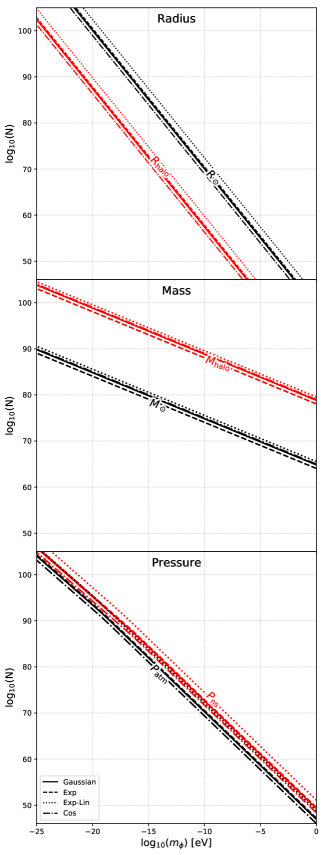
Figure 1: Plots of the Radii (top panel), Mass (middle panel) and Pressure (Bottom panel) for a Boson star. Red (and black) lines represent extreme high (low) values for each case, for the radii panel are a dark matter halo characteristic radius of $10^{14}$ Mpc, $R_{\rm halo}$ (in red), and the Solar radius, $R_{\odot}$ in black. In the case of the mass, we show contour lines for a solar mass, $M_{\odot}$ (in black), and a typical mass for dark matter halos $10^{12}\,M_{\odot}$ , $M_{\rm halo}$ (in red). For the pressure we show lines that represent the pressure of a neutron star $\mathcal{O}(10^{31})$ Pa, $P_{\rm ns}$ (in red), and 1 atmosphere of pressure, $P_{\rm atm}$ (in black). Different line–styles represent the different approximations, straight, dashed, dotted, dash–dotted represent the gaussian, linear–exponential, exponential and cosine, respectively.

If we assume that the pressure and gravity allows the BS to remain in equilibrium, then the following constraint to the number of particles is reached $N_{e}$,

$$N_{e}=\frac{\left(2\epsilon_{1}+\epsilon_{2}\right)}{12\pi\kappa\epsilon_{3}}\frac{R}{|a|},$$ (25)

where clearly $N$ is several orders of magnitud greater than $\kappa$. The scattering length, whose value can also be negative, should be only constrained from the particle physics model, this is, from Eq. (25) given a value for $a$ we should know the region where systems are not allowed to exist due to equilibrium. Clearly, if $N<N_{e}$ gravity overcome pressure and we could have an implosion of the system, if $N>N_{e}$ then pressure overcome gravity and apparently the system becomes unstable. $N_{e}$ allow us to find the systems that are in equilibrium, and stability condition will be study in a future work, where the rotation of the BS can be also included.

Alternatively to this scenario a phenomenological stability condition has been proposed in Ref. cornell for a trapped laboratory BEC. For a system with an attractive interaction, there is not enough kinetic energy to stabilize the BEC and it is expected to implode. A BEC can avoid implosion only as long as the number of atoms is less than a critical value given by

$$N_{c}=\gamma^{2}\frac{R}{|a|},$$ (26)

where the parameter $\gamma^{2}$ is the so–called stability coefficient and $R$ the size of the system. The the stability coefficient depends on the properties of the trapping potential, see Ref. cornell for details. Thus, according to our model the stability coefficient is in each case

$$\gamma^{2}=\frac{\left(2\epsilon_{1}+\epsilon_{2}\right)}{12\pi\kappa\epsilon_{3}}.$$ (27)

Introducing Eq. (26) into Eq. (24), we notice that the scattering length, $a$, must have positive sign, otherwise both terms in Eq. (24) are identical but opposite in sign. If $a>0$ the pressure simplifies as follows

$$P_{e}=\frac{\left(2\epsilon_{1}+\epsilon_{2}\right)^{2}}{24\pi^{2}\epsilon_{3}}\frac{\kappa\hbar^{2}}{am_{\phi}R_{e}^{4}},$$ (28)

where the subindex $e$ means that is evaluated at gravitational equilibrium, $N=N_{e}$.

To compute the equilibrium number of particles of the system, $N_{e}$, we still need to solve Eq. (26) because $R$ is function of the number of particles, $N$. Using $R=\kappa/\beta$ and Eq. (20) we have,

$$N_{e}=\left(\frac{(2\epsilon_{1}+\epsilon_{2})\hbar^{2}}{12\pi^{2}A\epsilon_{3}aGm_{\phi}^{3}\alpha}\right)^{1/2}.$$ (29)

then, the only free parameter is the scattering length, $a$.

		Gaussian	Exponential	Lin-Exp	Compact
Sun–like	$m_{\phi}$ [eV]	$1.29\times 10^{-12}$	$5.15\times 10^{-12}$	$8.51\times 10^{-12}$	$2.92\times 10^{-13}$
	N	$5.23\times 10^{76}$	$2.19\times 10^{75}$	$4.31\times 10^{76}$	$3.44\times 10^{77}$
	a [m]	$9.6\times 10^{-69}$	$3.96\times 10^{-67}$	$6.35\times 10^{-66}$	$2.47\times 10^{-63}$
	P [Pa]	$3.03\times 10^{12}$	$1.17\times 10^{11}$	$2.66\times 10^{12}$	$2.75\times 10^{20}$
Dwarf halo	$m_{\phi}$ [eV]	$1.35\times 10^{-22}$	$5.37\times 10^{-22}$	$8.87\times 10^{-22}$	$3.04\times 10^{-23}$
	N	$5.02\times 10^{94}$	$2.1\times 10^{93}$	$4.14\times 10^{94}$	$3.3\times 10^{95}$
	a [m]	$9.21\times 10^{-75}$	$3.8\times 10^{-73}$	$6.09\times 10^{-72}$	$2.37\times 10^{-69}$
	P [Pa]	$4.22\times 10^{-20}$	$1.62\times 10^{-21}$	$3.7\times 10^{-20}$	$3.83\times 10^{-12}$
Cluster halo	$m_{\phi}$ [eV]	$2.01\times 10^{-26}$	$8.02\times 10^{-26}$	$1.33\times 10^{-25}$	$4.54\times 10^{-27}$
	N	$3.36\times 10^{104}$	$1.41\times 10^{103}$	$2.77\times 10^{104}$	$2.21\times 10^{105}$
	a [m]	$6.17\times 10^{-83}$	$2.54\times 10^{-81}$	$4.08\times 10^{-80}$	$1.59\times 10^{-77}$
	P [Pa]	$1.05\times 10^{-14}$	$4.03\times 10^{-16}$	$9.17\times 10^{-15}$	$9.5\times 10^{-7}$

Table 2: Values to form a Sun–like or galaxy cluster halo system for the different ansätze the gaussian, the exponential, the linear exponential (Lin–Exp) and the compact. $m_{\phi}$ is the mass of the particle, $N$ is the number of particles, $a$ is the scattering length, and $P$ is the pressure of the system.

IV Numerical analysis

In Fig. 2, black lines represent systems in equilibrium, in all the figures we have taken two extreme examples. The dashed line is defined using $a_{\odot}$ is for a system of with a mass ($M_{e}=M_{\odot}$) and radius ($R_{e}=R_{\odot}$) as the Sun. Dash–dotted lines is for a system defined with the value of $a_{h}$ to represent a system of the size and mass of a typical cluster of dark matter halo, this is $M_{e}=10^{14}\;{\rm M_{\odot}}$ and $R_{e}=10^{3}$ kpc Newman:2012nv .

We find interesting that with only one parameter this approach can predict BECs of very different scales, and may be consider a fine–tuning problem to differentiate the value of the scattering length $a$. The larger value for $a$ is give to describe Sun–like systems and the compact hypothesis gives its largest values, which is of the order of $10^{-63}$ m. For each of the hypothesis taken, the values of $a$ is different depending if one wants to describe a Sun–like, dwarf DM halo, or a cluster DM halo system, see the Appendix A in which we show all the cases. It is interesting that, independent of the hypothesis taken, the value of $a_{sun}$ is 14 order of magnitud bigger than the case for the cluster dark matter halo, $a_{h}$.

Additionally, by using Eqns. (III), (24), and (29) we can find a relation between the pressure, $P$, and the energy density, $\varrho$, to compute the equation of state (EoS) of the type $P=\omega\varrho$. Thus, we obtain

$$\omega=\frac{1+\left(\frac{N}{N_{e}}\right)^{2}}{\frac{3(\epsilon_{1}+\epsilon_{2})}{2\epsilon_{1}+\epsilon_{2}}+\left(\frac{N}{N_{e}}\right)^{2}}\;\;.$$ (30)

When $N\gg N_{e}$ then $\omega\sim 1$ this may describe systems with properties know as a stiff matter, see for instance Ref. chavanis and references therein for details on this kind of schemes. For systems in equilibrium, Eq. (30) simplifies

$$\omega=\frac{1+\frac{2\epsilon_{1}}{\epsilon_{2}}}{2\left(1+\frac{5\epsilon_{1}}{4\epsilon_{2}}\right)},$$ (31)

then, for the gaussian and exponential case we have $\epsilon_{1}/\epsilon_{2}=1$, this is, $\omega=2/3$ describing an ideal system. For the exponential case $\epsilon_{1}/\epsilon_{2}=2/27$ and $\omega=31/59\approx 0.53$ and the compact case $\omega\approx 0.63$. Notice that for systems in equilibrium, the equation of state does not depend on any of the variables for the different models, and this also coincide with the fact that the scattering length, $a$, is very small, which reflect the nature of an ideal non–relativistic gas.

Despite the value of $\omega$ in the EoS, the fact that the pressure of the system, Eq. (28), depends on $a$ make possible to form halos in equilibrium of a galaxy cluster size with very small pressure, this characteristics resemble the properties of the dark matter. For instance, to form a system with the properties a dark matter halo that soround a galaxy cluster in the gaussian case we would need a scattering length of $a_{h}=6.17\times 10^{-83}$ m, a boson particle of mass $m_{\phi}=2.01\times 10^{-26}$ eV, and $N=3.36\times 10^{104}$ particles, and the BEC would have a pressure of $1.05\times 10^{-14}$ Pa, it is the extension of the condensate that makes it plausible to existence of this kind of systems.

To form system with mass and size of the Sun, for instance, we would need $N=5.23\times 10^{76}$ particles of mass $m_{\phi}=1.29\times 10^{-12}$ eV with an scattering length $a_{sun}=9.6\times 10^{-69}$ m. This Sun–like systems would have a pressure of $P_{e}=3.03\times 10^{1}2$ Pa. The shadowed areas In Fig. 2 represent systems with reasonable radii, mass and pressure for an astrophysical system. It is also interesting that systems with very high pressure can be found in this scheme, for instance, systems with $N=9.3\times 10^{91}$ particles with mass $m_{\phi}=8.0\times 10^{-18}$ eV and scattering length $a=9.6\times 10^{-84}$ m would have a pressure of $P=1.5\times 10^{31}$ Pa, which is of the order of the inner crust pressure of a neutron star 1603.02698 . However the approach we are proposing may not be valid to such a high pressures and relativistic corrections may have to be taken into account. Notice also that when quantum effects are taken into account, the pressure tends to zero at zero temperature for bosons pathria . Conversely, the equation of state $P=\varrho_{e}$ in which the pressure is proportional to the energy density $\rho_{e}$ is known in the literature as the so–called stiff matter, see for instance Ref. chavanis and references therein. We must mention that we are able to obtain apparently a stiff matter equation of state at $T=0$, even when our BS lies in the non–relativistic and low–density regime. The topics mentioned above deserves more in–depth analysis and will be presented elsewhere jaja .

Finally, several previous works Padilla:2020jdj ; Matos:2000ss ; Matos:2000ki ; Lora:2011yc ; RodriguezMontoya:2010zza ; Harko:2011zt ; Hu:2000ke have put constrains on the mass of scalar fields using galaxy rotation curves of dwarf galaxies since it is believe that the kinematic of this kind of systems is dominated by a DM halo. A typical size of the DM halo for a dwarf galaxy is of the order 22 kpc and have a total mass of the order of $10^{8}\;{\rm M_{\odot}}$ Kravtsov:2012jn ; Walker:2009zp . To form systems with this features we would need a boson particle with a mass of $m_{\phi}=1.35\times 10^{-22}$ eV and a scattering length $a=9.21\times 10^{-75}$ m, this is consistent within an order of magnitude with previous results, and it is consistent with the DM as dust hypothesis since the pressure is very small $P=4.22\times 10^{-20}$ Pa.

A relevant difference between anzats is the order of magnitude for the pressure of the systems in the compact scenario i.e., the compact ansatz, in which case is up to 9 orders of magnitude bigger than the exponential ansatz for the cluster halo and the Sun–like examples. It is seem to be that this discrepancy in the pressure between the compact and the non–compact ansätze relies on the choice for the corresponding BS’s radius $R=\beta^{-1}$, i.e., $\kappa=1$ for the compact ansatz, see Eq. (28). In other words, the results obtained in the present work agree with previous results reported in Ref. Joshua , which suggests that the case of the compact ansatz deserves deeper study and should be handled carefully.

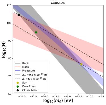
Figure 2: Contour plots where shaded regions may represent realistic astrophysical systems. Black region represents system of the size between $R_{\odot}$ and a typical dark matter halo in a galaxy cluster $10^{3}$ kpc. Red region represent system between a solar mass ($M_{\odot}$) and the mass of a dark matter halo in a galaxy cluster ($10^{14}\;M_{\odot}$). Blue region represent systems between 1 atmosphere and inner crust neutron star ($10^{31}$ Pa) pressure. Black lines are system in equilibrium given by Eq.(29), dashed (dash-dotted) line is taken $a$ for a Sun–like (dark matter halo kind) system. Yellow, green, and black dots represent the Sun, dwarf DM halo, and galaxy cluster dark matter halo system, respectively.

V Conclusions

We have analyzed a collection of non–relativistic gravitational bounded generic bosons forming a Bose–Einstein condensate starting from the single particle properties. We have also proved that the system can form stable structures in several scenarios that can be interpreted as BSs. By using four ansätze, the Gaussian, Exponential, the Linear exponential (non–compact ansatz), and the Cosine (compact ansatz), we are able to prove that they predict almost the same structural configuration, qualitatively speaking. Additionally, we have shown that different values of the corresponding scattering length, together with some specific values of the corresponding number of particles, lead to several sizes of BS in gravitational equilibrium. With our model, we can obtain from compact objects (i.e., the size of the sun, for instance) to gigantic configurations comparable to the size of galaxy cluster dark matter halos. In other words, our model predicts several configurations that may be stable and can form systems in gravitational equilibrium in a wide range of sizes. Notice that we are able to extract also significant properties associated with the BS thermodynamics. For instance, concerning the equation of state, we have calculated the corresponding ground state energy for each ansatz, from which we can obtain the corresponding internal energy and, consequently, the corresponding pressure. We can define two apparent limits according to the definition of the pressure $P=-\partial E_{0}/\partial V_{BS}$. The first one corresponds to the ideal case, i.e., $U_{0}=0$, and the second one at zero temperature. For the first case, we obtain that the equation of state is given by $P=\frac{2}{3}\frac{E_{0}}{V_{BS}}=\frac{2}{3}\varrho_{e}$. Conversely, at zero temperature (in which we can neglect the contributions of the kinetic energy) the equation of state can be expressed approximately as $P=\frac{E_{0}}{V_{BS}}=\varrho_{e}$. Let us remark that the aforementioned equations of state are irrespective of the considered ansatz. Notice that $P=\frac{2}{3}\varrho_{e}$ is the standard equation of state for an ideal non–relativistic bosonic system (it can be proved also that this is the equation of state for a system of ideal non–relativistic fermions in the classical regime pathria ). Additionally, when quantum effects are taken into account, the pressure also tends to zero at zero temperature for bosons pathria . Conversely, the equation of state $P=\varrho_{e}$ in which the pressure is proportional to the energy density $\varrho_{e}$ is known in the literature as the so–called stiff matter. We must mention that we are able to obtain apparently a stiff matter equation of state at $T=0$, even when our BS lies in the non–relativistic and low–density regime. The topics mentioned above deserves more in–depth analysis and will be presented elsewhere jaja . Finally, the present work must be extended to rotating systems in order to analyze the corresponding stability. Moreover, more general interactions within the system could be also relevant for compact objects, i.e., three–body interactions, and so on. Consequently, logarithmic interactions within a compact non–relativistic BS could be able to describe these scenarios. One more issue related to the BS configurations described in the present work is that they can be useful, in principle, to estimate the quantity of DM in the solar system. The topics mentioned above also deserve more in–depth analysis to study the eventual relation of BSs and DM as BECs of generic bosons in the universe.

Appendix A Plots

Here we present the contour plots for the exponential, linear-exponential and compact cases.

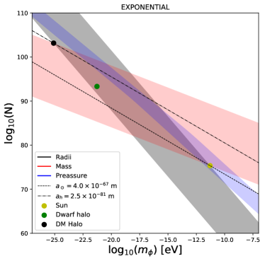
Figure 3: Contour plots for the exponential ansatz. Colors and styles are the same as in Fig.2.

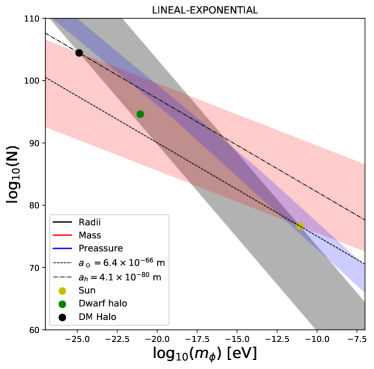
Figure 4: Contour plots for the linear-exponential ansatz. Colors and styles are the same as in Fig.2.

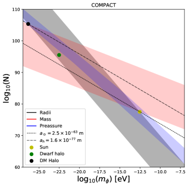
Figure 5: Contour plots for the compact ansatz. Colors and styles are the same as in Fig.2.

References

- (1) L. Dolan and R. Jackiw, Phys. Rev. D 9 (1974) 3320.
- (2) S. Weinberg, Phys. Rev. D 9 (1974) 3357.
- (3) E. Castellanos and T. Matos, Int. J. Mod. Phys. B 27 (2013) 11.
- (4) E. Castellanos, A. Macías and D. Nuñez, AIP Conf. Proc., Vol. 1577 (2014)
- (5) T. Matos and E. Castellanos, AIP Conf. Proc., Vol. 1577 (2014).
- (6) M. Grether, M. de Llano and G. A. Baker, Jr., Phys. Rev. Lett. 99 (2007) 200406.
- (7) S. Fagnocchi, S. Finazzi, S. Liberati, M. Kormos and A. Trombettoni, New J. Phys. 12 (2010) 095012.
- (8) Elías Castellanos, Celia Escamilla–Rivera, Alfredo Macías and Darío Nuñez, JCAP 11 (2014) 034.
- (9) S. J. Sin, Phys. Rev. D 50 (1994) 3650
- (10) S. U. Ji and S. J. Sin, Phys. Rev. D50 (1994) 3656
- (11) F. S. Guzmán, T. Matos and H. Villegas, Astron. Nachr. 320 (1999) 97
- (12) F. S. Guzmán and T. Matos, Class. Quantum Grav.17 (2000) L9
- (13) J. Magaña, T. Matos, J. Phys. Conf. Ser. 378 (2012) 012012.
- (14) Elías Castellanos, Juan Carlos Degollado, Claus Lammerzahl, Alfredo Macías and Volker Perlick, JCAP 01 (2018) 043.
- (15) Elías Castellanos, Celia Escamilla–Rivera and Jorge Mastache, Int. J. Mod. Phys. D. 29 9 (2020) 2050063.
- (16) J. Bernstein and S. Dodelson, Phys. Rev. Lett. 66 (1991) 683
- (17) L. Parker and Y. Zhang, Phys. Rev. D 44 (1991) 2421
- (18) C. G. Boehmer and T. Harko, JCAP (2007) 025
- (19) L.A. Ureña–López, JCAP (2009) 014
- (20) D.J. Kaup, Klein-Gordon geon, Phys. Rev. 172, 1331 (1968).
- (21) R. Ruffini and S. Bonazzola, Phys. Rev. 187, 1767 (1969).
- (22) S. Carignano, L. Lepori, A. Mammarella, M. Mannarelli, and G. Pagliaroli, Eur. Phys. J. A 53, 35 (2017).
- (23) F. Schunck and E. Mielke, Class. Quantum Grav. 20 (2003) R301-R356.
- (24) S. L. Liebling and C. Palenzuela, Living Rev. Relativity 15 (2012) 6.
- (25) Felix Kling and Arvind Rajaraman, Phys. Rev. D. 96 (2017) 044039.
- (26) Felix Kling and Arvind Rajaraman, Phys. Rev. Lett. 97 (2018) 063012.
- (27) C. J. Pethick and H. Smith, Bose-Einstein Condensation in Dilute Gases Cambridge University Press,Cambridge 2004.
- (28) F. Dalfovo, S. Giorgini, L. P. Pitaevskii and S. Stringari, Rev. Mod. Phys. 71 1999, 463-512.
- (29) M. Ueda, Fundamentals and New Frontiers of Bose–Einstein Condensation World Scientific, Singapore, 2010.
- (30) L. P. Pitaevskii and S. Stringari, Bose-Einstein Condensation, Clarendon Press, Oxford 2003.
- (31) S. Gutiérrez, B. Carvente and A. Camacho, Astrophys Space Sci 362 111 (2017).
- (32) S. Gutiérrez, B. Carvente, and A. Camacho, arXiv:1705.00087v1 [gr-qc] (2017).
- (33) J. Eby, et al., Phys. Rev. D 98 123013 (2018).
- (34) Joshua Eby, et. al. Journal of High Energy Physics 66 2016.
- (35) E. A. Donley, N. R. Claussen, S. L. Cornish, J. L. Roberts, E. A. Cornell and C. E. Wiemann, Nature 412 (2001) 295.
- (36) A. B. Newman, T. Treu, R. S. Ellis, D. J. Sand, C. Nipoti, J. Richard and E. Jullo, Astrophys. J. 765 (2013), 24 doi:10.1088/0004-637X/765/1/24 [arXiv:1209.1391 [astro-ph.CO]].
- (37) P. H. Chavanis, Eur. Phys. J. Plus 130 181 (2015).
- (38) Feryal Özel and Paulo Freire, Annual Review of Astronomy and Astrophysics, 54 (2016) 401-440.
- (39) R.K. Pathria, Statistical Mechanics, Butterworth Heineman, Oxford (1996).
- (40) Elías Castellanos, Guillermo Chacón–Acosta and Jorge Mastache. Ultra–cold Stiff matter Boson Stars. Work in progress.
- (41) W. Hu, R. Barkana and A. Gruzinov, Phys. Rev. Lett. 85 (2000), 1158-1161 doi:10.1103/PhysRevLett.85.1158 [arXiv:astro-ph/0003365 [astro-ph]].
- (42) T. Harko, Phys. Rev. D 83 (2011), 123515 doi:10.1103/PhysRevD.83.123515 [arXiv:1105.5189 [gr-qc]].
- (43) I. Rodriguez-Montoya, J. Magana, T. Matos and A. Perez-Lorenzana, Astrophys. J. 721 (2010), 1509-1514 doi:10.1088/0004-637X/721/2/1509 [arXiv:0908.0054 [astro-ph.CO]].
- (44) V. Lora, J. Magana, A. Bernal, F. J. Sanchez-Salcedo and E. K. Grebel, JCAP 02 (2012), 011 doi:10.1088/1475-7516/2012/02/011 [arXiv:1110.2684 [astro-ph.GA]].
- (45) T. Matos, F. S. Guzman and D. Nunez, Phys. Rev. D 62 (2000), 061301 doi:10.1103/PhysRevD.62.061301 [arXiv:astro-ph/0003398 [astro-ph]].
- (46) T. Matos and L. A. Urena-Lopez, Phys. Rev. D 63 (2001), 063506 doi:10.1103/PhysRevD.63.063506 [arXiv:astro-ph/0006024 [astro-ph]].
- (47) L. E. Padilla, J. Solís-López, T. Matos and A. Ávilez-López, [arXiv:2008.13455 [astro-ph.GA]].
- (48) M. G. Walker, M. Mateo, E. W. Olszewski, J. Penarrubia, N. W. Evans and G. Gilmore, Astrophys. J. 704 (2009), 1274-1287 [erratum: Astrophys. J. 710 (2010), 886-890] doi:10.1088/0004-637X/704/2/1274 [arXiv:0906.0341 [astro-ph.CO]].
- (49) A. V. Kravtsov, Astrophys. J. Lett. 764 (2013), L31 doi:10.1088/2041-8205/764/2/L31 [arXiv:1212.2980 [astro-ph.CO]].